Vector Calculus in Two Dimensions

by Peter J. Olver

University of Minnesota

1. Introduction.

The purpose of these notes is to review the basics of vector calculus in the two dimen-sions. We will assume you are familiar with the basics of partial derivatives, including theequality of mixed partials (assuming they are continuous), the chain rule, implicit differen-tiation. In addition, some familiarity with multiple integrals is assumed, although we willreview the highlights. Proofs and full details can be found in most vector calculus texts,including [1, 4].

We begin with a discussion of plane curves and domains. Many physical quantities,including force and velocity, are determined by vector fields, and we review the basicconcepts. The key differential operators in planar vector calculus are the gradient anddivergence operations, along with the Jacobian matrix for maps from R

2 to itself. Thereare three basic types of line integrals: integrals with respect to arc length, for computinglengths of curves, masses of wires, center of mass, etc., ordinary line integrals of vectorfields for computing work and fluid circulation, and flux line integrals for computing fluxof fluids and forces. Next, we review the basics of double integrals of scalar functionsover plane domains. Line and double integrals are connected by the justly famous Green’stheorem, which

2. Plane Curves.

We begin our review by collecting together the basic facts concerning geometry ofplane curves. A curve C ⊂ R

2 is parametrized by a pair of continuous functions

x(t) =

(x(t)y(t)

)∈ R

2, (2.1)

where the scalar parameter t varies over an (open or closed) interval I ⊂ R. When itexists, the tangent vector to the curve at the point x is described by the derivative,

dx

dt=

x =

(

x

y

). (2.2)

We shall often use Newton’s dot notation to abbreviate derivatives with respect to theparameter t.

Physically, we can think of a curve as the trajectory described by a particle moving inthe plane. The parameter t is identified with the time, and so x(t) gives the position of theparticle at time t. The tangent vector

x(t) measures the velocity of the particle at time t;

12/22/13 1 c© 2013 Peter J. Olver

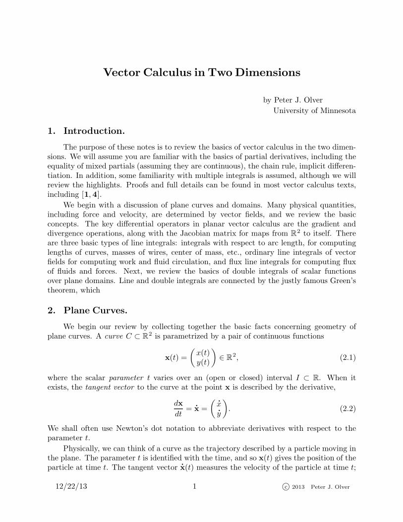
Cusped Curve Circle Figure Eight

Figure 1. Planar Curves.

its magnitude† ‖

x ‖ =√

x2 +

y2 is the speed, while its orientation (assuming the velocityis nonzero) indicates the instantaneous direction of motion of the particle as it movesalong the curve. Thus, by the orientation of a curve, we mean the direction of motion orparametrization, as indicated by the tangent vector. Reversing the orientation amountsto moving backwards along the curve, with the individual tangent vectors pointing in theopposite direction.

The curve parametrized by x(t) is called smooth provided its tangent vector is con-tinuous and everywhere nonzero:

x 6= 0. This is because curves with vanishing derivativemay have corners or cusps; a simple example is the first curve plotted in Figure 1, whichhas parametrization

x(t) =

(t2

t3

),

x(t) =

(2 t3 t2

),

and has a cusp at the origin when t = 0 and

x(0) = 0. Physically, a particle trajectoryremains smooth as long as the speed of the particle is never zero, which effectively preventsthe particle from instantaneously changing its direction of motion. A closed curve is smooth

if, in addition to satisfying

x(t) 6= 0 at all points a ≤ t ≤ b, the tangents at the endpointsmatch up:

x(a) =

x(b). A curve is called piecewise smooth if its derivative is piecewisecontinuous and nonzero everywhere. The corners in a piecewise smooth curve have well-defined right and left tangents. For example, polygons, such as triangles and rectangles,are piecewise smooth curves. In this book, all curves are assumed to be at least piecewisesmooth.

A curve is simple if it has no self-intersections: x(t) 6= x(s) whenever t 6= s. Physically,this means that the particle is never in the same position twice. A curve is closed if x(t)is defined for a ≤ t ≤ b and its endpoints coincide: x(a) = x(b), so that the particle endsup where it began. For example, the unit circle

x(t) = ( cos t, sin t )T

for 0 ≤ t ≤ 2π,

† Throughout, we always use the standard Euclidean inner product and norm. With somecare, all of the concepts can be adapted to other choices of inner product. In differential geometryand relativity, one even allows the inner product and norm to vary from point to point, [2].

12/22/13 2 c© 2013 Peter J. Olver

is closed and simple†, while the curve

x(t) = ( cos t, sin 2 t )T

for 0 ≤ t ≤ 2π,

is not simple since it describes a figure eight that intersects itself at the origin. Both curvesare illustrated in Figure 1.

Assuming the tangent vector

x(t) 6= 0, then the normal vector to the curve at thepoint x(t) is the orthogonal or perpendicular vector

x⊥ =

(

y−

x

)(2.3)

of the same length ‖

x⊥ ‖ = ‖

x ‖. Actually, there are two such normal vectors, the otherbeing the negative −

x⊥. We will always make the “right-handed” choice (2.3) of normal,meaning that as we traverse the curve, the normal always points to our right. If a simpleclosed curve C is oriented so that it is traversed in a counterclockwise direction — thestandard mathematical orientation — then (2.3) describes the outwards-pointing normal.If we reverse the orientation of the curve, then both the tangent vector and normal vectorchange directions; thus (2.3) would give the inwards-pointing normal for a simple closedcurve traversed in the clockwise direction.

The same curve C can be parametrized in many different ways. In physical terms, aparticle can move along a prescribed trajectory at a variety of different speeds, and thesecorrespond to different ways of parametrizing the curve. Conversion from one parame-trization x(t) to another x(τ) is effected by a change of parameter , which is a smooth,invertible function t = g(τ); the reparametrized curve is then x(τ) = x(g(τ)). We requirethat dt/dτ = g′(τ) > 0 everywhere. This ensures that each t corresponds to a uniquevalue of τ , and, moreover, the curve remains smooth and is traversed in the same overalldirection under the reparametrization. On the other hand, if g′(τ) < 0 everywhere, thenthe orientation of the curve is reversed under the reparametrization. We shall use thenotation −C to indicate the curve having the same shape as C, but with the reversedorientation.

Example 2.1. The function x(t) = ( cos t, sin t )T

for 0 < t < π parametrizes asemi-circle of radius 1 centered at the origin. If we set† τ = − cot t then we obtain the lessevident parametrization

x(τ) =

(1√

1 + τ2, − τ√

1 + τ2

)Tfor −∞ < τ <∞

of the same semi-circle, in the same direction. In the familiar parametrization, the velocityvector has unit length, ‖

x ‖ ≡ 1, and so the particle moves around the semicircle in thecounterclockwise direction with unit speed. In the second parametrization, the particle

† For a closed curve to be simple, we require x(t) 6= x(s) whenever t 6= s except at the ends,where x(a) = x(b) is required for the ends to close up.

† The minus sign is to ensure that dτ/dt > 0.

12/22/13 3 c© 2013 Peter J. Olver

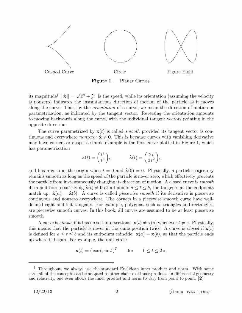
Interior Point Bounded Domain A Simple Closed Curve

Figure 2. Topology of Planar Domains.

slows down near the endpoints, and, in fact, takes an infinite amount of time to traversethe semicircle from right to left.

3. Planar Domains.

A plate or other two-dimensional body occupies a region in the plane, known as adomain. The simplest example is an open circular disk

Dr(a) =x ∈ R

2∣∣ ‖x− a ‖ < r

(3.1)

of radius r centered at a point a ∈ R2. In order to properly formulate the mathematical

tools needed to understand boundary value problems and dynamical equations for suchbodies, we first need to review basic terminology from point set topology of planar sets.Many of the concepts carry over as stated to subsets of any higher dimensional Euclideanspace R

n.

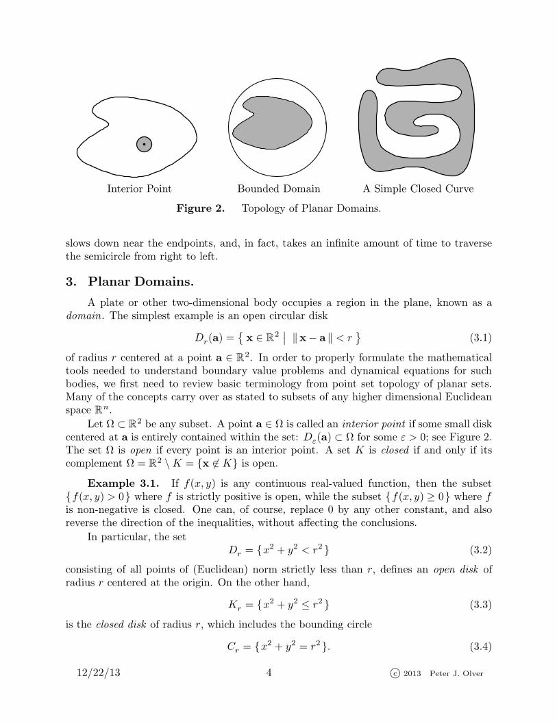
Let Ω ⊂ R2 be any subset. A point a ∈ Ω is called an interior point if some small disk

centered at a is entirely contained within the set: Dε(a) ⊂ Ω for some ε > 0; see Figure 2.The set Ω is open if every point is an interior point. A set K is closed if and only if itscomplement Ω = R

2 \K = x 6∈ K is open.

Example 3.1. If f(x, y) is any continuous real-valued function, then the subsetf(x, y) > 0 where f is strictly positive is open, while the subset f(x, y) ≥ 0 where fis non-negative is closed. One can, of course, replace 0 by any other constant, and alsoreverse the direction of the inequalities, without affecting the conclusions.

In particular, the setDr = x2 + y2 < r2 (3.2)

consisting of all points of (Euclidean) norm strictly less than r, defines an open disk ofradius r centered at the origin. On the other hand,

Kr = x2 + y2 ≤ r2 (3.3)

is the closed disk of radius r, which includes the bounding circle

Cr = x2 + y2 = r2 . (3.4)

12/22/13 4 c© 2013 Peter J. Olver

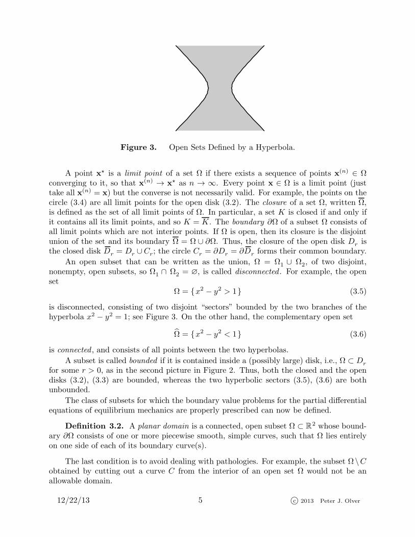
Figure 3. Open Sets Defined by a Hyperbola.

A point x⋆ is a limit point of a set Ω if there exists a sequence of points x(n) ∈ Ωconverging to it, so that x(n) → x⋆ as n → ∞. Every point x ∈ Ω is a limit point (justtake all x(n) = x) but the converse is not necessarily valid. For example, the points on thecircle (3.4) are all limit points for the open disk (3.2). The closure of a set Ω, written Ω,is defined as the set of all limit points of Ω. In particular, a set K is closed if and only ifit contains all its limit points, and so K = K. The boundary ∂Ω of a subset Ω consists ofall limit points which are not interior points. If Ω is open, then its closure is the disjointunion of the set and its boundary Ω = Ω ∪ ∂Ω. Thus, the closure of the open disk Dr isthe closed disk Dr = Dr ∪Cr; the circle Cr = ∂Dr = ∂Dr forms their common boundary.

An open subset that can be written as the union, Ω = Ω1 ∪ Ω2, of two disjoint,nonempty, open subsets, so Ω1 ∩ Ω2 = ∅, is called disconnected . For example, the openset

Ω = x2 − y2 > 1 (3.5)

is disconnected, consisting of two disjoint “sectors” bounded by the two branches of thehyperbola x2 − y2 = 1; see Figure 3. On the other hand, the complementary open set

Ω = x2 − y2 < 1 (3.6)

is connected , and consists of all points between the two hyperbolas.

A subset is called bounded if it is contained inside a (possibly large) disk, i.e., Ω ⊂ Drfor some r > 0, as in the second picture in Figure 2. Thus, both the closed and the opendisks (3.2), (3.3) are bounded, whereas the two hyperbolic sectors (3.5), (3.6) are bothunbounded.

The class of subsets for which the boundary value problems for the partial differentialequations of equilibrium mechanics are properly prescribed can now be defined.

Definition 3.2. A planar domain is a connected, open subset Ω ⊂ R2 whose bound-

ary ∂Ω consists of one or more piecewise smooth, simple curves, such that Ω lies entirelyon one side of each of its boundary curve(s).

The last condition is to avoid dealing with pathologies. For example, the subset Ω\Cobtained by cutting out a curve C from the interior of an open set Ω would not be anallowable domain.

12/22/13 5 c© 2013 Peter J. Olver

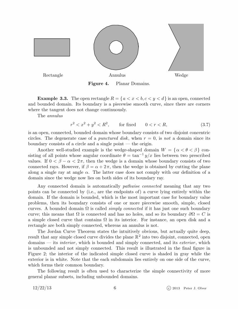
Rectangle Annulus Wedge

Figure 4. Planar Domains.

Example 3.3. The open rectangle R = a < x < b, c < y < d is an open, connectedand bounded domain. Its boundary is a piecewise smooth curve, since there are cornerswhere the tangent does not change continuously.

The annulus

r2 < x2 + y2 < R2, for fixed 0 < r < R, (3.7)

is an open, connected, bounded domain whose boundary consists of two disjoint concentriccircles. The degenerate case of a punctured disk , when r = 0, is not a domain since itsboundary consists of a circle and a single point — the origin.

Another well-studied example is the wedge-shaped domain W = α < θ < β con-sisting of all points whose angular coordinate θ = tan−1 y/x lies between two prescribedvalues. If 0 < β − α < 2π, then the wedge is a domain whose boundary consists of twoconnected rays. However, if β = α+ 2π, then the wedge is obtained by cutting the planealong a single ray at angle α. The latter case does not comply with our definition of adomain since the wedge now lies on both sides of its boundary ray.

Any connected domain is automatically pathwise connected meaning that any twopoints can be connected by (i.e., are the endpoints of) a curve lying entirely within thedomain. If the domain is bounded, which is the most important case for boundary valueproblems, then its boundary consists of one or more piecewise smooth, simple, closedcurves. A bounded domain Ω is called simply connected if it has just one such boundarycurve; this means that Ω is connected and has no holes, and so its boundary ∂Ω = C isa simple closed curve that contains Ω in its interior. For instance, an open disk and arectangle are both simply connected, whereas an annulus is not.

The Jordan Curve Theorem states the intuitively obvious, but actually quite deep,result that any simple closed curve divides the plane R2 into two disjoint, connected, opendomains — its interior , which is bounded and simply connected, and its exterior , whichis unbounded and not simply connected. This result is illustrated in the final figure inFigure 2; the interior of the indicated simple closed curve is shaded in gray while theexterior is in white. Note that the each subdomain lies entirely on one side of the curve,which forms their common boundary.

The following result is often used to characterize the simple connectivity of moregeneral planar subsets, including unbounded domains.

12/22/13 6 c© 2013 Peter J. Olver

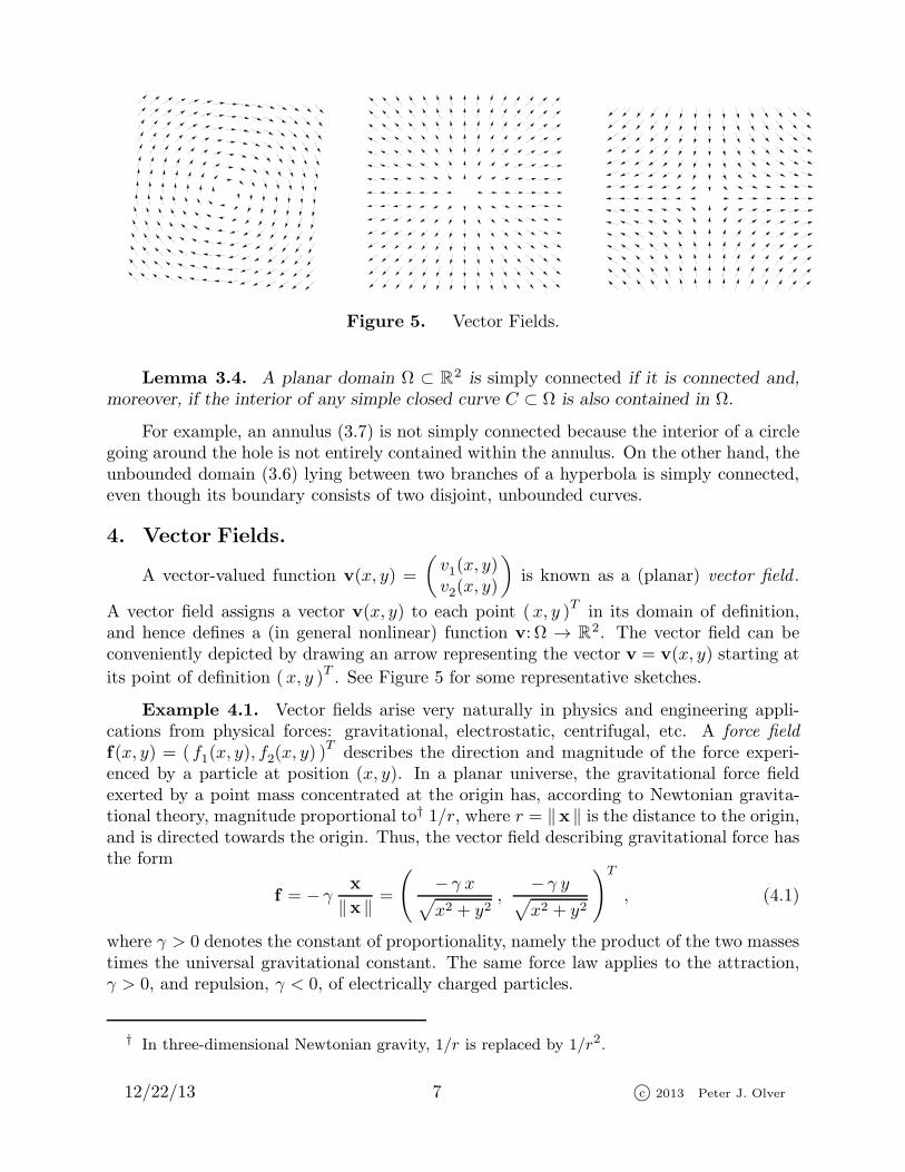
Figure 5. Vector Fields.

Lemma 3.4. A planar domain Ω ⊂ R2 is simply connected if it is connected and,

moreover, if the interior of any simple closed curve C ⊂ Ω is also contained in Ω.

For example, an annulus (3.7) is not simply connected because the interior of a circlegoing around the hole is not entirely contained within the annulus. On the other hand, theunbounded domain (3.6) lying between two branches of a hyperbola is simply connected,even though its boundary consists of two disjoint, unbounded curves.

4. Vector Fields.

A vector-valued function v(x, y) =

(v1(x, y)v2(x, y)

)is known as a (planar) vector field .

A vector field assigns a vector v(x, y) to each point (x, y )T

in its domain of definition,and hence defines a (in general nonlinear) function v: Ω → R

2. The vector field can beconveniently depicted by drawing an arrow representing the vector v = v(x, y) starting at

its point of definition ( x, y )T. See Figure 5 for some representative sketches.

Example 4.1. Vector fields arise very naturally in physics and engineering appli-cations from physical forces: gravitational, electrostatic, centrifugal, etc. A force field

f(x, y) = ( f1(x, y), f2(x, y) )T

describes the direction and magnitude of the force experi-enced by a particle at position (x, y). In a planar universe, the gravitational force fieldexerted by a point mass concentrated at the origin has, according to Newtonian gravita-tional theory, magnitude proportional to† 1/r, where r = ‖x ‖ is the distance to the origin,and is directed towards the origin. Thus, the vector field describing gravitational force hasthe form

f = − γx

‖x ‖ =

(− γ x√x2 + y2

,− γ y√x2 + y2

)T, (4.1)

where γ > 0 denotes the constant of proportionality, namely the product of the two massestimes the universal gravitational constant. The same force law applies to the attraction,γ > 0, and repulsion, γ < 0, of electrically charged particles.

† In three-dimensional Newtonian gravity, 1/r is replaced by 1/r2.

12/22/13 7 c© 2013 Peter J. Olver

Newton’s Laws of planetary motion produce the second order system of differentialequations

md2x

dt2= f .

The solutions x(t) describe the trajectories of planets subject to a central gravitationalforce, e.g., the sun. They also govern the motion of electrically charged particles under acentral electric charge, e.g., classical (i.e., not quantum) electrons revolving around a cen-tral nucleus. In three-dimensional Newtonian mechanics, planets move along conic sections— ellipses in the case of planets, and parabolas and hyperbolas in the case of non-recurrentobjects like some comets. Interestingly (and not as well-known), the corresponding two-dimensional theory is not as neatly described — the typical orbit of a planet around aplanar sun does not form a simple closed curve, [3]!

Example 4.2. Another important example is the velocity vector field v of a steady-state fluid flow. The vector v(x, y) measures the instantaneous velocity of the fluid particles(molecules or atoms) as they pass through the point (x, y). “Steady-state” means thatthe velocity at a point (x, y) does not vary in time — even though the individual fluidparticles are in motion. If a fluid particle moves along the curve x(t) = (x(t), y(t))T , thenits velocity at time t is the derivative v =

x of its position with respect to t. Thus, fora time-independent velocity vector field v(x, y) = ( v1(x, y), v2(x, y) )

T, the fluid particles

will move in accordance with an autonomous, first order system of ordinary differentialequations

dx

dt= v1(x, y),

dy

dt= v2(x, y). (4.2)

According to the basic theory of systems of ordinary differential equations , an individualparticle’s motion x(t) will be uniquely determined solely by its initial position x(0) = x0.In fluid mechanics, the trajectories of particles are known as the streamlines of the flow.The velocity vector v is everywhere tangent to the streamlines. When the flow is steady,the streamlines do not change in time. Individual fluid particles experience the samemotion as they successively pass through a given point in the domain occupied by thefluid.

As a specific example, consider the vector field

v(x, y) =

(−ω yω x

), (4.3)

for fixed ω > 0, which is plotted in the first figure in Figure 5. The corresponding fluidtrajectories are found by solving the associated first order system of ordinary differentialequations

x = −ω y,

y = ω x,

with initial conditions x(0) = x0, y(0) = y0. This is a linear system, and can be solved bythe eigenvalue and eigenvector techniques presented in [6; Chapter 9]. The resulting flow

x(t) = x0 cosω t− y0 sinω t, y(t) = x0 sinω t+ y0 cosω t,

12/22/13 8 c© 2013 Peter J. Olver

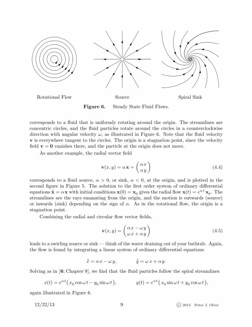
Rotational Flow Source Spiral Sink

Figure 6. Steady State Fluid Flows.

corresponds to a fluid that is uniformly rotating around the origin. The streamlines areconcentric circles, and the fluid particles rotate around the circles in a counterclockwisedirection with angular velocity ω, as illustrated in Figure 6. Note that the fluid velocityv is everywhere tangent to the circles. The origin is a stagnation point, since the velocityfield v = 0 vanishes there, and the particle at the origin does not move.

As another example, the radial vector field

v(x, y) = αx =

(αxαy

)(4.4)

corresponds to a fluid source, α > 0, or sink, α < 0, at the origin, and is plotted in thesecond figure in Figure 5. The solution to the first order system of ordinary differentialequations

x = αx with initial conditions x(0) = x0 gives the radial flow x(t) = eαt x0. Thestreamlines are the rays emanating from the origin, and the motion is outwards (source)or inwards (sink) depending on the sign of α. As in the rotational flow, the origin is astagnation point.

Combining the radial and circular flow vector fields,

v(x, y) =

(αx− ωyωx+ αy

)(4.5)

leads to a swirling source or sink — think of the water draining out of your bathtub. Again,the flow is found by integrating a linear system of ordinary differential equations

x = αx− ω y,

y = ω x+ αy.

Solving as in [6; Chapter 9], we find that the fluid particles follow the spiral streamlines

x(t) = eαt(x0 cosω t− y0 sinω t

), y(t) = eαt

(x0 sinω t+ y0 cosω t

),

again illustrated in Figure 6.

12/22/13 9 c© 2013 Peter J. Olver

Remark : Of course, physical fluid motion occurs in three-dimensional space. However,any planar flow can also be viewed as a particular type of three-dimensional fluid motionthat does not depend upon the vertical coordinate. The motion on every horizontal planeis the same, and so the planar flow represents a cross-section of the full three-dimensionalmotion. For example, slicing a steady flow past a vertical cylinder by a transverse horizontalplane results in a planar flow around a circle.

5. Gradient and Curl.

In the same vein, a scalar-valued function u(x, y) is often referred to as a scalar

field , since it assigns a scalar to each point (x, y )T

in its domain of definition. Typicalphysical examples of scalar fields include temperature, deflection of a membrane, height ofa topographic map, density of a plate, and so on.

The gradient operator ∇ maps a scalar field u(x, y) to the vector field

∇u = gradu =

(∂u/∂x∂u/∂y

)(5.1)

consisting of its two first order partial derivatives. The scalar field u is often referred toas a potential function for its gradient vector field ∇u. For example, the gradient of thepotential function u(x, y) = x2 + y2 is the radial vector field ∇u = ( 2x, 2y )

T. Similarly,

the gradient of the logarithmic potential function

u(x, y) = − γ log r = − 12γ log(x2 + y2)

is the gravitational force (4.1) exerted by a point mass concentrated at the origin. Addi-tional physical examples include the velocity potential of certain fluid velocity vector fieldsand the electromagnetic potential whose gradient describes the electromagnetic force field.

Not every vector field admits a potential because not every vector field lies in therange of the gradient operator ∇. Indeed, if u(x, y) has continuous second order partialderivatives, and (

v1v2

)= v = ∇u =

(uxuy

),

then, by the equality of mixed partials,

∂v1∂y

=∂

∂y

(∂u

∂x

)=

∂

∂x

(∂u

∂y

)=∂v2∂x

.

The resulting equation∂v1∂y

=∂v2∂x

(5.2)

constitutes one of the necessary conditions that a vector field must satisfy in order to bea gradient. Thus, for example, the rotational vector field (4.3) does not satisfy (5.2), andhence is not a gradient. There is no potential function for such circulating flows.

12/22/13 10 c© 2013 Peter J. Olver

The difference between the two terms in (5.2) is known as the curl of the planar vectorfield v = (v1, v2), and denoted by†

∇ ∧ v = curlv =∂v2∂x

− ∂v1∂y

. (5.3)

Notice that the curl of a planar vector field is a scalar field. (In contrast, in three dimen-sions, the curl of a vector field is a vector field, [1, 4].) Thus, a necessary condition for avector field to be a gradient is that its curl vanish identically: ∇ ∧ v ≡ 0.

Even if the vector field has zero curl, it still may not be a gradient. Interestingly, thegeneral criterion depends only upon the topology of the domain of definition, as clarifiedin the following theorem.

Theorem 5.1. Let v be a smooth vector field defined on a domain Ω ⊂ R2. If

v = ∇u for some scalar function u, then ∇ ∧ v ≡ 0. If Ω is simply connected, then the

converse holds: if ∇ ∧ v ≡ 0 then v = ∇u for some potential function u defined on Ω.

As we shall see, this result is a direct consequence of Green’s Theorem 8.1.

Example 5.2. The vector field

v =

( −yx2 + y2

,x

x2 + y2

)T(5.4)

satisfies ∇ ∧ v ≡ 0. However, there is no potential function defined for all (x, y) 6= (0, 0)such that ∇u = v. As the reader can check, the angular coordinate

u = θ = tan−1 y

x(5.5)

satisfies ∇θ = v, but θ is not well-defined on the entire domain since it experiences a jumpdiscontinuity of magnitude 2π as we go around the origin. Indeed, Ω = x 6= 0 is not

simply connected, and so Theorem 5.1 does not apply. On the other hand, if we restrictv to any simply connected subdomain Ω ⊂ Ω that does not encircle the origin, then theangular coordinate (5.5) can be unambiguously and smoothly defined on Ω, and does serveas a single-valued potential function for v.

In fluid mechanics, the curl of a vector field measures the local circulation in theassociated steady state fluid flow. If we place a small paddle wheel in the fluid, then itsrate of spinning will be in proportion to ∇ ∧ v. (An explanation of this fact will appearbelow.) The fluid flow is called irrotational if its velocity vector field has zero curl, andhence, assuming Ω is simply connected, is a gradient: v = ∇u. In this case, the paddlewheel will not spin. The scalar function u(x, y) is known as the velocity potential forthe fluid motion. Similarly, a force field that is given by a gradient f = ∇ϕ is called aconservative force field , and the function ϕ defines the force potential.

† In this text, we adopt the more modern wedge notation ∧ for what is often denoted by across ×.

12/22/13 11 c© 2013 Peter J. Olver

Suppose u(x) = u(x, y) is a scalar field. Given a parametrized curve x(t) = (x(t), y(t) )T,

the composition f(t) = u(x(t)) = u(x(t), y(t)) indicates the behavior as we move alongthe curve. For example, if u(x, y) represents the elevation of a mountain range at position(x, y), and x(t) represents our position at time t, then f(t) = u(x(t)) is our altitude at timet. Similarly, if u(x, y) represents the temperature at (x, y), then f(t) = u(x(t)) measuresour temperature at time t.

The rate of change of the composite function is found through the chain rule

df

dt=

d

dtu(x(t), y(t)) =

∂u

∂x

dx

dt+

∂u

∂y

dy

dt= ∇u ·

x, (5.6)

and hence equals the dot product between the gradient ∇u(x(t)) and the tangent vector

x(t) to the curve at the point x(t). For instance, our rate of ascent or descent as wetravel through the mountains is given by the dot product of our velocity vector with thegradient of the elevation function. The dot product between the gradient and a fixed vectora = ( a, b )

Tis known as the directional derivative of the scalar field u(x, y) in the direction

a, and denoted by∂u

∂a= a · ∇u = aux + buy. (5.7)

Thus, the rate of change of u along a curve x(t) is given by its directional derivative∂u/∂

x = ∇u ·

x, as in (5.6), in the tangent direction. This leads us to one importantinterpretation of the gradient vector.

Proposition 5.3. The gradient ∇u of a scalar field points in the direction of steepest

increase of u. The negative gradient, −∇u, which points in the opposite direction, indicates

the direction of steepest decrease of u.

For example, if u(x, y) represents the elevation of a mountain range at position (x, y)on a map, then ∇u tells us the direction that is steepest uphill, while −∇u points directlydownhill — the direction water will flow. Similarly, if u(x, y) represents the temperature ofa two-dimensional body, then ∇u tells us the direction in which it gets hottest the fastest.Heat energy (like water) will flow in the opposite direction, namely in the direction of thevector −∇u. This basic fact underlies the derivation of the multi-dimensional heat anddiffusion equations.

You need to be careful in how you interpret Proposition 5.3. Clearly, the faster youmove along a curve, the faster the function u(x, y) will vary, and one needs to take thisinto account when comparing the rates of change along different curves. The easiest wayto normalize is to assume that the tangent vector a =

x has norm 1, so ‖ a ‖ = 1 and weare going through x with unit speed. Once this is done, Proposition 5.3 is an immediateconsequence of the Cauchy–Schwarz inequality. Indeed,

∣∣∣∣∂u

∂a

∣∣∣∣ = | a · ∇u | ≤ ‖ a ‖ ‖∇u ‖ = ‖∇u ‖, when ‖ a ‖ = 1,

with equality if and only if a = c∇u points in the same direction as the gradient. Therefore,the maximum rate of change is when a = ∇u/‖∇u ‖ is the unit vector in the direction ofthe gradient, while the minimum is achieved when a = −∇u/‖∇u ‖ points in the opposite

12/22/13 12 c© 2013 Peter J. Olver

direction. As a result, Proposition 5.3 tells us how to move if we wish to minimize a scalarfunction as rapidly as possible.

Theorem 5.4. A curve x(t) will realize the steepest decrease in the scalar field u(x)if and only if it satisfies the gradient flow equation

x = −∇u, or

dx

dt= − ∂u

∂x(x, y),

dy

dt= − ∂u

∂y(x, y).

(5.8)

The only points at which the gradient does not tell us about the directions of in-crease/decrease are the critical points , which are, by definition, points where the gradientvanishes: ∇u = 0. These include local maxima or minima of the function, i.e., mountainpeaks or bottoms of valleys, as well as other types of critical points like saddle points thatrepresent mountain passes. In such cases, we must look at the second or higher orderderivatives to tell the directions of increase/decrease.

Remark : Theorem 5.4 forms the basis of gradient descent methods for numericallyapproximating the maxima and minima of functions. One begins with a guess (x0, y0)for the minimum and then follows the gradient flow in to the minimum by numericallyintegrating the system of ordinary differential equations (5.8).

Example 5.5. Consider the function u(x, y) = x2 + 2y2. Its gradient vector field is

∇u = ( 2x, 4y )T, and hence the gradient flow equations (5.8) take the form

x = −2x,

y = −4y.

The solution that starts out at initial position (x0, y0 )Tis

x(t) = x0 e−2 t, y(t) = y0 e

−4 t. (5.9)

Note that the origin is a stable fixed point for this linear dynamical system, and thesolutions x(t) → 0 converge exponentially fast to the minimum of the function u(x, y). Ifwe start out not on either of the coordinate axes, so x0 6= 0 and y0 6= 0, then the trajectory(5.9) is a semi-parabola of the form y = cx2, where c = y0/x

20. These curves, along with

the four coordinate semi-axes, are the paths to follow to get to the minimum 0 the fastest.

Level Sets

Let u(x, y) be a scalar field. The curves defined by the implicit equation

u(x, y) = c (5.10)

holding the function u(x, y) constant are known as its level sets . For instance, if u(x, y)represents the elevation of a mountain range, then its level sets are the usual contour lineson a topographic map. The Implicit Function Theorem tells us that, away from criticalpoints, the level sets of a planar function are simple, though not necessarily closed, curves.

12/22/13 13 c© 2013 Peter J. Olver

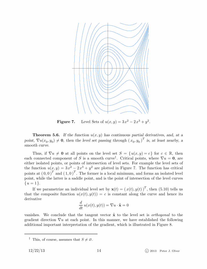
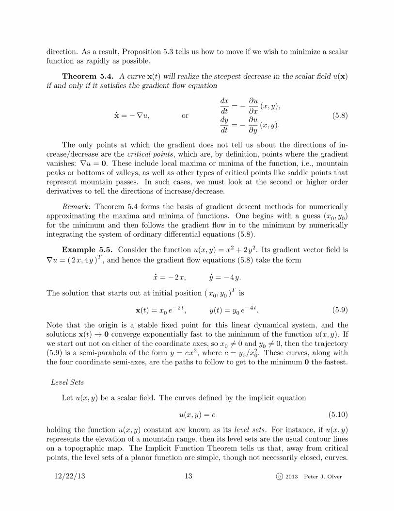
Figure 7. Level Sets of u(x, y) = 3x2 − 2x3 + y2.

Theorem 5.6. If the function u(x, y) has continuous partial derivatives, and, at a

point, ∇u(x0, y0) 6= 0, then the level set passing through ( x0, y0 )T

is, at least nearby, a

smooth curve.

Thus, if ∇u 6= 0 at all points on the level set S = u(x, y) = c for c ∈ R, theneach connected component of S is a smooth curve†. Critical points, where ∇u = 0, areeither isolated points, or points of intersection of level sets. For example the level sets ofthe function u(x, y) = 3x2 − 2x3 + y2 are plotted in Figure 7. The function has critical

points at ( 0, 0 )Tand ( 1, 0 )

T. The former is a local minimum, and forms an isolated level

point, while the latter is a saddle point, and is the point of intersection of the level curvesu = 1.

If we parametrize an individual level set by x(t) = (x(t), y(t) )T, then (5.10) tells us

that the composite function u(x(t), y(t)) = c is constant along the curve and hence itsderivative

d

dtu(x(t), y(t)) = ∇u ·

x = 0

vanishes. We conclude that the tangent vector

x to the level set is orthogonal to thegradient direction ∇u at each point. In this manner, we have established the followingadditional important interpretation of the gradient, which is illustrated in Figure 8.

† This, of course, assumes that S 6= ∅.

12/22/13 14 c© 2013 Peter J. Olver

∇u

Figure 8. Level Sets and Gradient.

Theorem 5.7. The gradient ∇u of a scalar field u is everywhere orthogonal to its

level sets u = c.

Comparing Theorems 5.4 and 5.7, we conclude that the curves of steepest descentare always orthogonal (perpendicular) to the level sets of the function. Thus, if we wantto hike uphill the fastest, we should keep our direction of travel always perpendicular tothe contour lines. Similarly, if u(x, y) represents temperature in a planar body at position(x, y) then the level sets are the curves of constant temperature, known as the isotherms .Heat energy will flow in the negative gradient direction, and hence orthogonally to theisotherms.

Example 5.8. Consider again the function u(x, y) = x2 + 2y2 from Example 5.5.Its level sets u(x, y) = x2 + 2y2 = c form a system of concentric ellipses centered at theorigin. Theorem 5.7 implies that the parabolic trajectories (5.9) followed by the solutionsto the gradient flow equations form an orthogonal system of curves to the ellipses. This isevident in Figure 9, showing that the ellipses and parabolas intersect everywhere at rightangles.

6. Integrals on Curves.

As you know, integrals of scalar functions,

∫ b

a

f(t) dt, are taken along real intervals

[a, b ] ⊂ R. In higher dimensional calculus, there are a variety of possible types of integrals.The closest in spirit to one-dimensional integration are “line† integrals”, in which oneintegrates along a curve. In planar calculus, line integrals come in three flavors. The most

† A more accurate term would be “curve integral”, but the terminology is standard and willnot be altered in this text.

12/22/13 15 c© 2013 Peter J. Olver

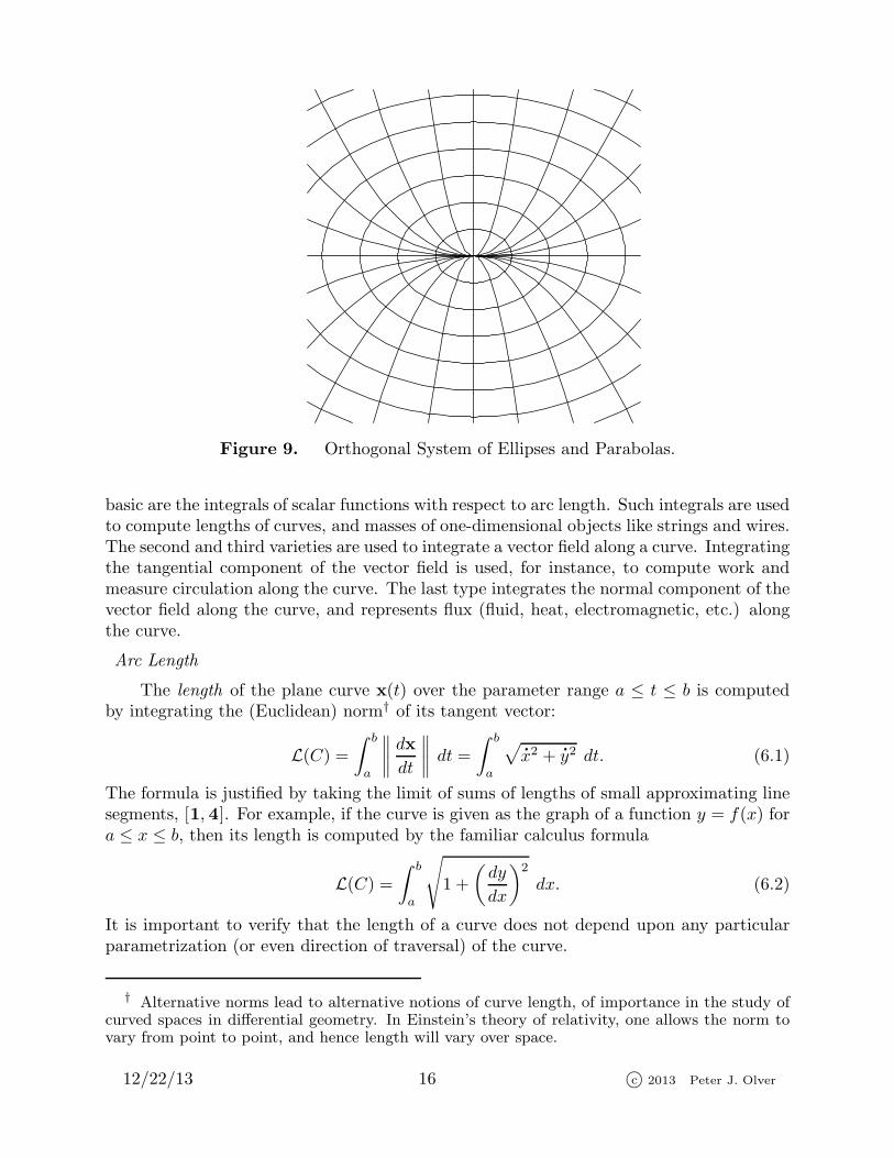
Figure 9. Orthogonal System of Ellipses and Parabolas.

basic are the integrals of scalar functions with respect to arc length. Such integrals are usedto compute lengths of curves, and masses of one-dimensional objects like strings and wires.The second and third varieties are used to integrate a vector field along a curve. Integratingthe tangential component of the vector field is used, for instance, to compute work andmeasure circulation along the curve. The last type integrates the normal component of thevector field along the curve, and represents flux (fluid, heat, electromagnetic, etc.) alongthe curve.

Arc Length

The length of the plane curve x(t) over the parameter range a ≤ t ≤ b is computedby integrating the (Euclidean) norm† of its tangent vector:

L(C) =∫ b

a

∥∥∥∥dx

dt

∥∥∥∥ dt =∫ b

a

√

x2 +

y2 dt. (6.1)

The formula is justified by taking the limit of sums of lengths of small approximating linesegments, [1, 4]. For example, if the curve is given as the graph of a function y = f(x) fora ≤ x ≤ b, then its length is computed by the familiar calculus formula

L(C) =∫ b

a

√1 +

(dy

dx

)2

dx. (6.2)

It is important to verify that the length of a curve does not depend upon any particularparametrization (or even direction of traversal) of the curve.

† Alternative norms lead to alternative notions of curve length, of importance in the study ofcurved spaces in differential geometry. In Einstein’s theory of relativity, one allows the norm tovary from point to point, and hence length will vary over space.

12/22/13 16 c© 2013 Peter J. Olver

Example 6.1. The length of a circle x(t) =

(r cos tr sin t

), 0 ≤ t ≤ 2π, of radius r is

given by

L(C) =∫ 2π

0

∥∥∥∥dx

dt

∥∥∥∥ dt =∫ 2π

0

r dt = 2πr,

verifying the well-known formula for its circumference. On the other hand, the curve

x(t) =

(a cos tb sin t

), 0 ≤ t ≤ 2π, (6.3)

parametrizes an ellipse with semi-axes a, b. Its arc length is given by the integral

s =

∫ 2π

0

√a2 sin2t+ b2 cos2 t dt.

Unfortunately, this integral cannot be expressed in terms of elementary functions. It is, infact, an elliptic integral , [5], so named for this very reason!

A curve is said to be parametrized by arc length, written x(s) = ( x(s), y(s) )T, if one

traverses it with constant, unit speed, which means that∥∥∥∥dx

ds

∥∥∥∥ = 1 (6.4)

at all points. In other words, the length of that part of the curve between arc lengthparameter values s = s0 and s = s1 is exactly equal to s1 − s0. To convert from a moregeneral parameter t to arc length s = σ(t), we must compute

s = σ(t) =

∫ t

a

∥∥∥∥dx

dt

∥∥∥∥ dt and so ds = ‖

x ‖ dt =√

x2 +

y2 dt. (6.5)

The unit tangent to the curve at each point is obtained by differentiating with respectto the arc length parameter:

t =dx

ds=

x

‖

x ‖ =

(

x√

x2 +

y2,

y√

x2 +

y2

), so that ‖ t ‖ = 1. (6.6)

(As always, we require

x 6= 0.) The unit normal to the curve is orthogonal to the unittangent,

n = t⊥ =

(dy

ds,− dx

ds

)=

(

y√

x2 +

y2,

−

x√

x2 +

y2

), so that

‖n ‖ = 1,

n · t = 0.(6.7)

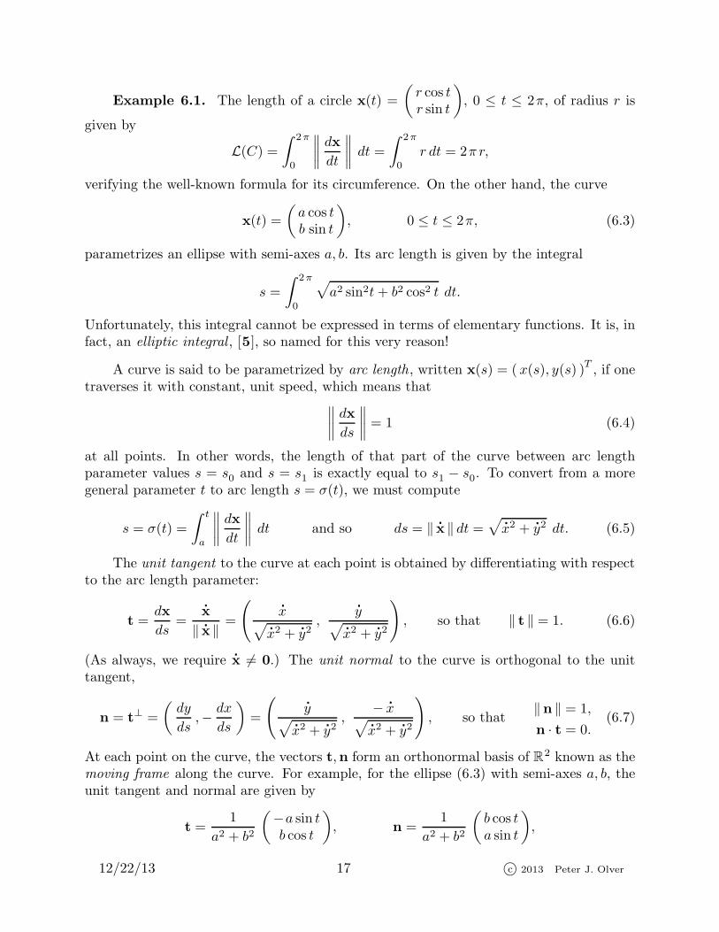
At each point on the curve, the vectors t,n form an orthonormal basis of R2 known as themoving frame along the curve. For example, for the ellipse (6.3) with semi-axes a, b, theunit tangent and normal are given by

t =1

a2 + b2

(−a sin tb cos t

), n =

1

a2 + b2

(b cos ta sin t

),

12/22/13 17 c© 2013 Peter J. Olver

nt

Figure 10. The Moving Frame for an Ellipse.

and graphed in Figure 10. Actually, a curve has two unit normals at each point — onepoints to our right side and the other to our left side as we move along the curve. Thenormal n in (6.7) is the right-handed normal, and is the traditional one to choose; theopposite, left-handed normal is its negative −n. If we traverse a simple closed curve ina counterclockwise direction, then the right-handed normal n is the unit outward normal,pointing to the curve’s exterior.

Arc Length Integrals

We now explain how to integrate scalar functions along curves. Suppose first that Cis a (piecewise) smooth curve that is parametrized by arc length, x(s) = (x(s), y(s)) for0 ≤ s ≤ ℓ, where ℓ is the total length of C. If u(x) = u(x, y) is any scalar field, we defineits arc length integral along the curve C to be

∫

C

u ds =

∫ ℓ

0

u(x(s), y(s))ds. (6.8)

For example, if ρ(x, y) represents the density at position (x, y) of a wire bent in the shape

of a curve C, then the arc length integral

∫

C

ρ(x, y)ds computes the total mass of the wire.

In particular, the length of the curve is (tautologously) given by

L(C) =∫

C

ds =

∫ ℓ

0

ds = ℓ. (6.9)

If we use an alternative parametrization x(t), with a ≤ t ≤ b, then the arc length integralis computed using the change of parameter formula (6.5), and so

∫

C

u ds =

∫ b

a

u(x(t))

∥∥∥∥dx

dt

∥∥∥∥ dt =∫ b

a

u(x(t), y(t))

√(dx

dt

)2

+

(dy

dt

)2

dt. (6.10)

Changing the orientation of the curve does not alter the value of this type of line integral.Moreover, if we break up the curve into two nonoverlapping pieces, then the arc lengthintegral decomposes into a sum:

∫

C

u ds =

∫

−Cu ds,

∫

C

u ds =

∫

C1

u ds +

∫

C2

u ds, C = C1 ∪ C2. (6.11)

12/22/13 18 c© 2013 Peter J. Olver

Example 6.2. A circular wire radius 1 has density proportional to the distance ofthe point from the x axis. The mass of the wire is computed by the arc length integral

∮

C

| y | ds =∫ 2π

0

| sin t | dt = 4.

The arc length integral was evaluated using the parametrization x(t) = ( a cos t, a sin t )T

for 0 ≤ t ≤ 2π, whereby ds = ‖

x ‖ dt = dt.

Line Integrals of Vector Fields

There are two intrinsic ways of integrating a vector field along a curve. In the firstversion, we integrate its tangential component v · t, where t = dx/ds is the unit tangentvector, with respect to arc length.

Definition 6.3. The line integral of a vector field v along a parametrized curve x(t)is given by ∫

C

v · dx =

∫

C

v1(x, y) dx+ v2(x, y) dy =

∫

C

v · t ds. (6.12)

To evaluate the line integral, we parametrize the curve by x(t) for a ≤ t ≤ b, and then

∫

C

v · dx =

∫ b

a

v(x(t)) · dxdtdt =

∫ b

a

[v1(x(t), y(t))

dx

dt+ v2(x(t), y(t))

dy

dt

]dt. (6.13)

This result follows from the formulae (6.5, 6) for the arc length and unit tangent vector. Ingeneral, line integrals are independent of how the curve is parametrized — as long as it istraversed in the same direction. Reversing the direction of parameterization, i.e., changingthe orientation of the curve, changes the sign of the line integral — because it reverses thedirection of the unit tangent. As before, line integrals can be decomposed into sums overcomponents:∫

−Cv · dx = −

∫

C

v · dx,∫

C

v · dx =

∫

C1

v · dx +

∫

C2

v · dx, C = C1 ∪ C2.

(6.14)In the second formula, one must take care to orient the two parts C1, C2 in the samedirection as C.

Example 6.4. Let C denote the circle of radius r centered at the origin. We willcompute the line integral of the rotational vector field (5.4), namely

∮

C

v · dx =

∮

C

y dx− x dy

x2 + y2.

The circle on the integral sign serves to remind us that we are integrating around a closedcurve. We parameterize the circle by

x(t) = r cos t, y(t) = r sin t, 0 ≤ t ≤ 2π.

12/22/13 19 c© 2013 Peter J. Olver

Applying the basic line integral formula (6.13), we find

∮

C

y dx− x dy

x2 + y2=

∫ 2π

0

− r2 sin2 t− r2 cos2 t

r2dt = −2π,

independent of the circle’s radius. Note that the parametrization goes around the circleonce in the counterclockwise direction. If we go around once in the clockwise direction,e.g., by using the parametrization x(t) = (r sin t, r cos t), then the resulting line integralequals +2π.

If v represents the velocity vector field of a steady state fluid, then the line integral(6.12) represents the circulation of the fluid around the curve. Indeed, v · t is proportionalto the force exerted by the fluid in the direction of the curve, and so the circulation integralmeasures the average of the tangential fluid forces around the curve. Thus, for example,the rotational vector field (5.4) has a net circulation of −2π around any circle centered atthe origin. The minus sign tells us that the fluid is circulating in the clockwise direction— opposite to the direction in which we went around the circle.

A fluid flow is irrotational if the circulation is zero for all closed curves. An irrotationalflow will not cause a paddle wheel to rotate — there will be just as much fluid pushing inone direction as in the opposite, and the net tangential forces will cancel each other out.The connection between circulation and the curl of the velocity vector field will be madeevident shortly.

If the vector field happens to be the gradient of a scalar field, then we can readilyevaluate its line integral.

Theorem 6.5. If v = ∇u is a gradient vector field, then its line integral

∫

C

∇u · dx = u(b)− u(a) (6.15)

equals the difference between the potential function’s values at the endpoints a = x(a)and b = x(b) of the curve C.

Corollary 6.6. Let Ω be a connected domain. A scalar field has zero gradient,

∇u(x, y) = 0, for all (x, y )T ∈ Ω, if and only if u(x, y) ≡ c is constant on Ω.

Proof : Indeed,, if a,b are any two points in Ω, then, by connectivity, we can finda curve connecting them. Then (6.15) implies that u(b) = u(a), which shows that u isconstant. Q.E.D.

Thus, the line integral of a gradient field is independent of path; its value does notdepend on how you get from point a to point b. In particular, if C is a closed curve, then

∮

C

∇u · dx = 0,

since the endpoints coincide: a = b. In fact, independence of path is both necessary andsufficient for the vector field to be a gradient.

12/22/13 20 c© 2013 Peter J. Olver

Theorem 6.7. Let v be a vector field defined on a domain Ω. Then the following

are equivalent:

(a) The line integral

∫

C

v · dx is independent of path.

(b)

∮

C

v · dx = 0 for every closed curve C.

(c) v = ∇u is the gradient of some potential function defined on Ω.

In such cases, on any connected component, a potential function can be computed byintegrating the vector field

u(x) =

∫x

a

v · dx. (6.16)

Here a is any fixed point (which defines the zero potential level), and we evaluate theline integral over any curve that connects a to x; path-independence says that it does notmatter which curve we use to get from a to x. The proof that ∇u = v is left as an exercise.

Example 6.8. The line integral∫

C

v · dx =

∫

C

(x2 − 3y) dx+ (2− 3x) dy

of the vector field v =(x2 − 3y, 2− 3x

)Tis independent of path. Indeed, parametrizing

a curve C by (x(t), y(t)), a ≤ t ≤ b, leads to

∫

C

(x2 − 3y) dx+ (2− 3x) dy =

∫ b

a

[(x2 − 3y)

dx

dt+ (2− 3x)

dy

dt

]dt

=

∫ b

a

d

dt

(x3 − 3xy + 2y

)dt =

(x3 − 3xy + 2y

) ∣∣∣∣b

t=a

.

The result only depends on the endpoints a = ( x(a), y(a) )T, b = ( x(b), y(b) )

T, and not

on the detailed shape of the curve. Integrating from a = 0 to b = (x, y) produces thepotential function

u(x, y) = x3 − 3xy + 2y.

As guaranteed by (6.16), ∇u = v.

On the other hand, the line integral∫

C

v · dx =

∫

C

(x3 − 2y) dx+ x2 dy

of the vector field v =(x3 − 2y, x2

)Tis not path-independent, and so v does not admit a

potential function. Indeed, integrating from (0, 0) to (1, 1) along the straight line segment (t, t) | 0 ≤ t ≤ 1 , produces

∫

C

(x3 − 2y) dx+ x2 dy =

∫ 1

0

(t3 − 2 t+ t2

)dt = − 5

12 .

12/22/13 21 c© 2013 Peter J. Olver

On the other hand, integrating along the parabola (t, t2) | 0 ≤ t ≤ 1 , yields a differentvalue ∫

C

(x3 − 2y) dx+ x2 dy =

∫ 1

0

(t3 − 2 t2 + 2 t3

)dt = 1

12 .

If v represents a force field, then the line integral (6.12) represents the amount ofwork required to move along the given curve. Work is defined as force, or, more correctly,the tangential component of the force in the direction of motion, times distance. Theline integral effectively totals up the infinitesimal contributions, the sum total representingthe total amount of work expended in moving along the curve. Note that the work isindependent of the parametrization of the curve. In other words (and, perhaps, counter-intuitively†), the amount of work expended doesn’t depend upon how fast you move alongthe curve.

According to Theorem 6.7, the work does not depend on the route you use to get fromone point to the other if and only if the force field admits a potential function: v = ∇u.Then, by (6.15), the work is just the difference in potential at the two points. In particular,for a gradient vector field there is no net work required to go around a closed path.

Flux

The second type of line integral is found by integrating the normal component of thevector field along the curve: ∫

C

v · n ds. (6.17)

Using the formula (6.7) for the unit normal, we find that the inner product can be rewrittenin the alternative form

v · n = v1dy

ds− v2

dx

ds= v⊥ · t ,

where t = dx/ds is the unit tangent, while

v⊥ = (−v2, v1 )T

(6.18)

is a vector field that is everywhere orthogonal to the velocity vector field v = ( v1, v2 )T.

Thus, the normal line integral (6.17) can be rewritten as a tangential line integral

∫

C

v · n ds =

∫

C

v1 dy − v2 dx =

∫

C

v ∧ dx =

∫

C

v⊥ · dx =

∫

C

v⊥ · t ds. (6.19)

If v represents the velocity vector field for a steady-state fluid flow, then the innerproduct v · n with the unit normal measures the flux of the fluid flow across the curve atthe given point. The flux is positive if the fluid is moving in the normal direction n and

† The reason this doesn’t agree with our intuition about work is that we are not taking frictionaleffects into account, and these are typically velocity-dependent.

12/22/13 22 c© 2013 Peter J. Olver

negative if it is moving in the opposite direction. If the vector field admits a potential,v = ∇u, then the flux

v · n = ∇u · n =∂u

∂n(6.20)

equals its normal derivative, i.e., the directional derivative of the potential function u in

the normal direction to the curve. The line integral

∫

C

v · n ds sums up the individual

fluxes, and so represents the total flux across the curve, meaning the total volume of fluidthat passes across the curve per unit time — in the direction assigned by the unit normaln. In particular, if C is a simple closed curve and n is the outward normal, then theflux integral (6.17) measures the net outflow of fluid across C; if negative, it represents aninflow. The total flux is zero if and only if the total amount of fluid contained within thecurve does not change. Thus, in the absence of sources or sinks, an incompressible fluid,such as water, will have zero net flux around any closed curve since the total amount offluid within any given region cannot change.

Example 6.9. For the radial vector field

v = x =

(xy

), we have v⊥ =

(−yx

).

As we saw in Example 4.2, v represents the fluid flow due to a source at the origin. Thus,the resulting fluid flux across a circle C of radius r is computed using the line integral

∮

C

v · n ds =∮

C

x dy − y dx =

∫ 2π

0

r2 sin2 t+ r2 cos2 t dt = 2π r2.

Therefore, the source fluid flow has a net outflow of 2π r2 units across a circle of radius r.This is not an incompressible flow!

7. Double Integrals.

We assume that the student is familiar with the foundations of multiple integration,and merely review a few of the highlights in this section. Given a scalar function u(x, y)defined on a domain Ω, its double integral

∫ ∫

Ω

u(x, y)dx dy =

∫ ∫

Ω

u(x) dx (7.1)

is equal to the volume of the solid lying underneath the graph of u over Ω. If u(x, y)represents the density at position (x, y)T in a plate having the shape of the domain Ω,then the double integral (7.1) measures the total mass of the plate. In particular,

area Ω =

∫ ∫

Ω

dx dy

is equal to the area of the domain Ω.

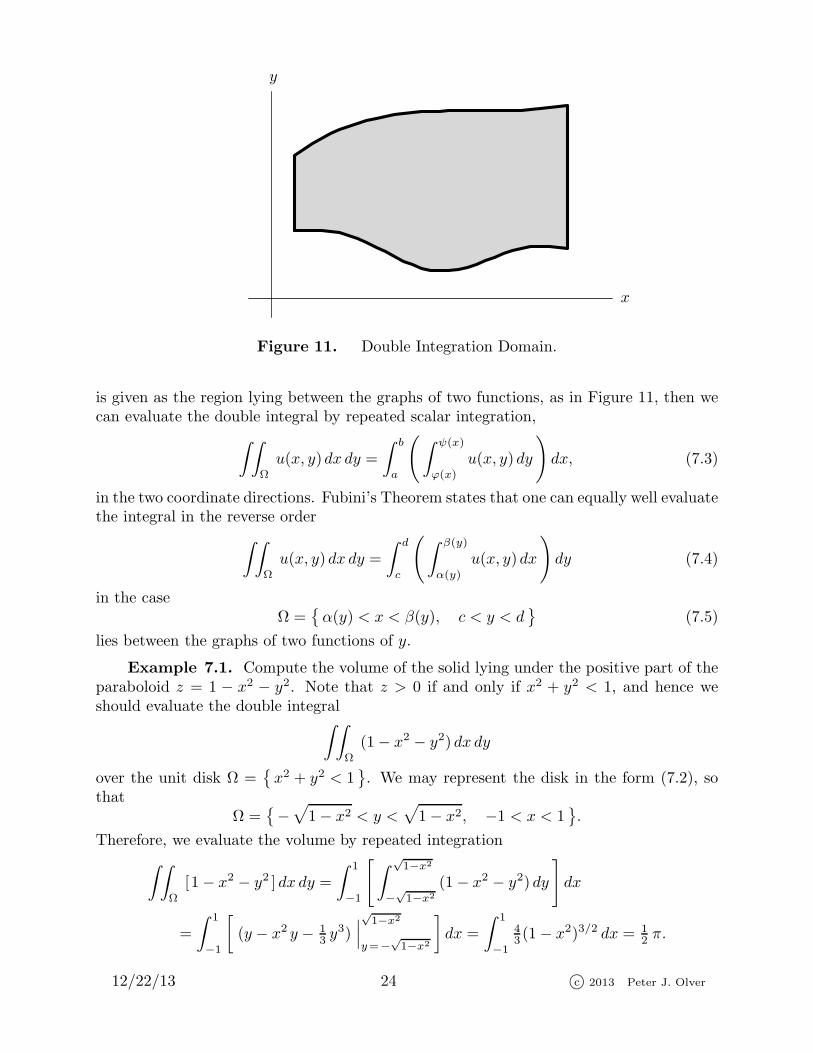
In the particular case when

Ω =ϕ(x) < y < ψ(x), a < x < b

(7.2)

12/22/13 23 c© 2013 Peter J. Olver

x

y

Figure 11. Double Integration Domain.

is given as the region lying between the graphs of two functions, as in Figure 11, then wecan evaluate the double integral by repeated scalar integration,

∫ ∫

Ω

u(x, y)dx dy =

∫ b

a

(∫ ψ(x)

ϕ(x)

u(x, y)dy

)dx, (7.3)

in the two coordinate directions. Fubini’s Theorem states that one can equally well evaluatethe integral in the reverse order

∫ ∫

Ω

u(x, y)dx dy =

∫ d

c

(∫ β(y)

α(y)

u(x, y)dx

)dy (7.4)

in the caseΩ =

α(y) < x < β(y), c < y < d

(7.5)

lies between the graphs of two functions of y.

Example 7.1. Compute the volume of the solid lying under the positive part of theparaboloid z = 1 − x2 − y2. Note that z > 0 if and only if x2 + y2 < 1, and hence weshould evaluate the double integral

∫ ∫

Ω

(1− x2 − y2) dx dy

over the unit disk Ω =x2 + y2 < 1

. We may represent the disk in the form (7.2), so

thatΩ =

−√

1− x2 < y <√1− x2, −1 < x < 1

.

Therefore, we evaluate the volume by repeated integration

∫ ∫

Ω

[1− x2 − y2 ] dx dy =

∫ 1

−1

[∫ √1−x2

−√1−x2

(1− x2 − y2) dy

]dx

=

∫ 1

−1

[(y − x2 y − 1

3 y3)∣∣∣√1−x2

y=−√1−x2

]dx =

∫ 1

−1

43 (1− x2)3/2 dx = 1

2 π.

12/22/13 24 c© 2013 Peter J. Olver

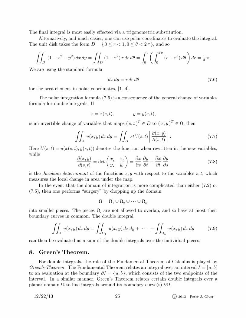
The final integral is most easily effected via a trigonometric substitution.

Alternatively, and much easier, one can use polar coordinates to evaluate the integral.The unit disk takes the form D = 0 ≤ r < 1, 0 ≤ θ < 2π, and so

∫ ∫

D

(1− x2 − y2) dx dy =

∫ ∫

D

(1− r2) r dr dθ =

∫ 1

0

(∫ 2π

0

(r − r3) dθ

)dr = 1

2 π.

We are using the standard formula

dx dy = r dr dθ (7.6)

for the area element in polar coordinates, [1, 4].

The polar integration formula (7.6) is a consequence of the general change of variablesformula for double integrals. If

x = x(s, t), y = y(s, t),

is an invertible change of variables that maps ( s, t )T ∈ D to (x, y )

T ∈ Ω, then

∫ ∫

Ω

u(x, y)dx dy =

∫ ∫

D

stU(s, t)

∣∣∣∣∂(x, y)

∂(s, t)

∣∣∣∣ . (7.7)

Here U(s, t) = u(x(s, t), y(s, t)) denotes the function when rewritten in the new variables,while

∂(x, y)

∂(s, t)= det

(xs xtys yt

)=∂x

∂s

∂y

∂t− ∂x

∂t

∂y

∂s(7.8)

is the Jacobian determinant of the functions x, y with respect to the variables s, t, whichmeasures the local change in area under the map.

In the event that the domain of integration is more complicated than either (7.2) or(7.5), then one performs “surgery” by chopping up the domain

Ω = Ω1 ∪ Ω2 ∪ · · · ∪ Ωk

into smaller pieces. The pieces Ωi are not allowed to overlap, and so have at most theirboundary curves in common. The double integral

∫ ∫

Ω

u(x, y)dx dy =

∫ ∫

Ω1

u(x, y)dx dy + · · · +

∫ ∫

Ωk

u(x, y)dx dy (7.9)

can then be evaluated as a sum of the double integrals over the individual pieces.

8. Green’s Theorem.

For double integrals, the role of the Fundamental Theorem of Calculus is played byGreen’s Theorem. The Fundamental Theorem relates an integral over an interval I = [a, b ]to an evaluation at the boundary ∂I = a, b, which consists of the two endpoints of theinterval. In a similar manner, Green’s Theorem relates certain double integrals over aplanar domain Ω to line integrals around its boundary curve(s) ∂Ω.

12/22/13 25 c© 2013 Peter J. Olver

Theorem 8.1. Let v(x) be a smooth vector field defined on a bounded domain

Ω ⊂ R2. Then the line integral of v around the boundary ∂Ω equals the double integral of

the curl of v over the domain. This result can be written in either of the equivalent forms

∫ ∫

Ω

∇∧ v dx =

∮

∂Ω

v · dx,∫ ∫

Ω

(∂v2∂x

− ∂v1∂y

)dx dy =

∮

∂Ω

v1 dx+ v2 dy . (8.1)

Green’s Theorem was first formulated in 1828 by the English mathematician andmiller George Green, and, contemporaneously, by the Russian mathematician MikhailOstrogradski.

Example 8.2. Let us apply Green’s Theorem 8.1 to the particular vector fieldv = ( 0, x )

T. Since ∇ ∧ v ≡ 1, we find

∮

∂Ω

x dy =

∫ ∫

Ω

dx dy = area Ω. (8.2)

This means that we can compute the area of a planar domain by computing the indicatedline integral around its boundary! For example, to compute the area of a disk Dr of radius

r, we parametrize its bounding circle Cr by ( r cos t, r sin t )Tfor 0 ≤ t ≤ 2π, and compute

area Dr =

∮

Cr

x dy =

∫ 2π

0

r2 cos2 t dt = πr2.

If we interpret v as the velocity vector field associated with a steady state fluid flow,then the right hand side of formula (8.1) represents the circulation of the fluid around theboundary of the domain Ω. Green’s Theorem implies that the double integral of the curlof the velocity vector must equal this circulation line integral.

If we divide the double integral in (8.1) by the area of the domain,

1

area Ω

∫ ∫

Ω

∇∧ v dx = MΩ [∇∧ v ] ,

we obtain the mean of the curl ∇ ∧ v of the vector field over the domain. In particular,if the domain Ω is very small, then ∇ ∧ v does not vary much, and so its value at anypoint in the domain is more or less equal to the mean. On the other hand, the right handside of (8.1) represents the circulation around the boundary ∂Ω. Thus, we conclude thatthe curl ∇ ∧ v of the velocity vector field represents an “infinitesimal circulation” at thepoint it is evaluated. In particular, the fluid is irrotational, with no net circulation aroundany curve, if and only if ∇ ∧ v ≡ 0 everywhere. Under the assumption that its domain ofdefinition is simply connected, Theorem 6.7 tell us that this is equivalent to the existenceof a velocity potential u with ∇u = v.

Theorem 8.3. A vector field v defined on a simply connected domain Ω ⊂ R2

admits a potential, v = ∇ϕ for some ϕ: Ω → R if and only if ∇ ∧ v ≡ 0.

12/22/13 26 c© 2013 Peter J. Olver

We can also apply Green’s Theorem 8.1 to flux line integrals of the form (6.17). Usingthe identification (6.19) followed by (8.1), we find that

∮

∂Ω

v · n ds =∮

∂Ω

v⊥ · dx =

∫ ∫

Ω

∇∧ v⊥ dx dy.

However, note that the curl of the orthogonal vector field (6.18), namely

∇∧ v⊥ =∂v1∂x

+∂v2∂y

= ∇ · v, (8.3)

coincides with the divergence of the original velocity field. Combining these together, wehave proved the divergence or flux form of Green’s Theorem:

∫ ∫

Ω

∇ · v dx dy =

∮

∂Ω

v · n ds. (8.4)

As before, Ω is a bounded domain, and n is the unit outward normal to its boundary ∂Ω.

In the fluid flow interpretation, the right hand side of (8.4) represents the net fluidflux out of the region Ω. Thus, the double integral of the divergence of the flow vectormust equal this net change in area. Thus, in the absence of sources or sinks, the divergenceof the velocity vector field, ∇·v will represent the local change in area of the fluid at eachpoint. In particular, if the fluid is incompressible if and only if ∇ · v ≡ 0 everywhere.

An ideal fluid flow is both incompressible, ∇ · v = 0, and irrotational, ∇ ∧ v = 0.Assuming its domain is simply connected, we introduce velocity potential u(x, y), so that∇u = v. Therefore,

0 = ∇ · v = ∇ · ∇u = uxx + uyy. (8.5)

Therefore, the velocity potential for an incompressible, irrotational fluid flow is a harmonicfunction, i.e., it satisfies the Laplace equation. Water waves are typically modeled inthis manner, and so many problems in fluid mechanics rely on the solution to Laplace’sequation.

References

[1] Apostol, T.M., Calculus, Blaisdell Publishing Co., Waltham, Mass., 1967–69.

[2] Boothby, W.M., An Introduction to Differentiable Manifolds and Riemannian

Geometry, Academic Press, New York, 1975.

[3] Dewdney, A.K., The Planiverse. Computer Contact with a Two-dimensional World,Copernicus, New York, 2001.

[4] Marsden, J.E., and Tromba, A.J., Vector Calculus, 4th ed., W.H. Freeman, NewYork, 1996.

[5] Olver, F.W.J., Lozier, D.W., Boisvert, R.F., and Clark, C.W., eds., NIST Handbook

of Mathematical Functions, Cambridge University Press, Cambridge, 2010.

[6] Olver, P.J., and Shakiban, C., Applied Linear Algebra, Prentice–Hall, Inc., UpperSaddle River, N.J., 2006.

12/22/13 27 c© 2013 Peter J. Olver