Vector-based Navigation using Grid-like Representations1

in Artificial Agents.2

Andrea Banino1,2,3∗, Caswell Barry2∗, Benigno Uria1, Charles Blundell1, Timothy Lillicrap1,3

Piotr Mirowski1, Alexander Pritzel1, Martin J. Chadwick1, Thomas Degris1, Joseph Modayil1,4

Greg Wayne1, Hubert Soyer1, Fabio Viola1, Brian Zhang1, Ross Goroshin1, Neil Rabinowitz1,5

Razvan Pascanu1, Charlie Beattie1, Stig Petersen1, Amir Sadik1, Stephen Gaffney1, Helen King1,6

Koray Kavukcuoglu1, Demis Hassabis1,4, Raia Hadsell1, Dharshan Kumaran1,37

1DeepMind, 5 New Street Square, London EC4A 3TW, UK.8

2Department of Cell and Developmental Biology, University College London, London, UK9

3Centre for Computation, Mathematics and Physics in the Life Sciences and Experimental Biology10

(CoMPLEX), University College London, London, UK11

4Gatsby Computational Neuroscience Unit, 25 Howland Street, London W1T 4JG, UK12

∗equal contribution.13

Deep neural networks have achieved impressive successes in diverse areas ranging from ob-14

ject recognition to complex games such as Go1, 2. Navigation, however, remains a substantial15

challenge for artificial agents, with deep neural networks trained by reinforcement learn-16

ing (RL)3–5 failing to rival the proficiency of mammalian spatial behavior, underpinned by17

grid cells in the entorhinal cortex6. Grid cells are viewed to provide a multi-scale periodic18

representation that functions as a metric for coding space7, 8 which is critical for integrat-19

ing self-motion (path integration)6, 7, 9 and planning direct trajectories to goals (vector-based20

navigation)7, 10, 11. We set out to leverage the computational functions of grid cells to develop a21

deep RL agent with mammalian-like navigational abilities. We first trained a recurrent net-22

work to perform path integration, leading to the emergence of representations resembling23

grid cells, as well as other entorhinal cell types12. We then showed that this representation24

1

provided an effective basis for an agent to locate goals in complex, unfamiliar, and change-25

able environments — optimizing the primary objective of navigation through deep RL. The26

performance of agents endowed with grid-like representations surpassed that of an expert27

human and comparison agents, with the metric quantities necessary for vector-based nav-28

igation derived from grid-like units within the network. Further, grid-like representations29

enabled agents to conduct shortcut behaviours reminiscent of those performed by mammals.30

Our findings show that emergent grid-like representations furnish agents with a Euclidean31

spatial metric and associated vector operations, providing a foundation for proficient nav-32

igation. As such, our results support neuro-scientific theories that see grid cells as critical33

for vector-based navigation7, 10, 11, demonstrating that the latter can be combined with path-34

based strategies to support navigation in complex environments.35

The ability to self-localize in the environment and update one's position on the basis of self-36

motion are core components of navigation13. We trained a deep neural network to path integrate37

within a square arena (2.2m×2.2m), using simulated trajectories modelled on those of foraging ro-38

dents (see Methods). The network was required to update its estimate of location and head direction39

based on translational and angular velocity signals, mirroring those available to the mammalian40

brain12, 14, 15 (see Methods, Fig. 1a&b). Velocity was provided as input to a recurrent network41

with a Long Short-Term Memory architecture (LSTM) which was trained using backpropagation42

through time (see Methods and Supplemental Discussion), allowing the network to dynamically43

combine current input signals with activity patterns reflecting past events (see Methods, Fig. 1a).44

The LSTM projected to place and head direction units via a linear layer — units with activity45

2

defined as a simple linear function of their input (see Extended Data Figure 1 for architecture).46

Importantly, the linear layer was subject to regularization, in particular dropout16, such that 50% of47

the units were randomly silenced at each time step. The vector of activities in the place and head48

direction units, corresponding to the current position, was provided as a supervised training signal49

at each time step (see Methods and Extended Data Figure 1). This form of supervision follows50

evidence that in mammals, place and head direction representations exist in close anatomical prox-51

imity to entorhinal grid cells12 and emerge in rodent pups prior to the appearance of mature grid52

cells17, 18. Equally, in adult rodents, entorhinal grid cells are known to project to the hippocampus1953

and appear to contribute to the neural activity of place cells19.54

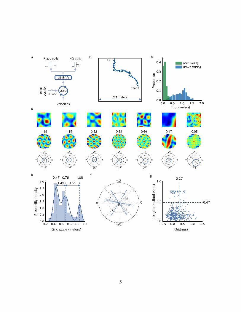
As expected, the network was able to path integrate accurately in this setting involving for-55

aging behavior (mean error after 15s trajectory, 16cm vs 91cm for an untrained network, effect56

size = 2.83; 95% CI [2.80, 2.86], Fig. 1b&c). Strikingly, individual units within the linear layer57

of the network developed stable spatial activity profiles similar to neurons within the entorhinal58

network6, 12 (Fig. 1d, Extended Data Figure 2). Specifically, 129 of the 512 linear layer units59

(25.2%) resembled grid cells, exhibiting significant hexagonal periodicity (gridness20) versus a60

null distribution generated by a conservative fields shuffling procedure (see Methods). The scale61

of the grid-patterns, measured from the spatial autocorrelograms of the activity maps20, varied62

between units (range 28cm to 115cm, mean 66cm) and followed a multi-modal distribution, con-63

sistent with empirical results from rodent grid cells21, 22 (Fig. 1e). To assess these clusters we64

fit mixtures of Gaussians, finding the most parsimonious number by minimizing the Bayesian In-65

formation Criterion (BIC). The distribution was best fit by 3 Gaussians (means 47cm, 70cm, and66

3

106cm), indicating the presence of scale clusters with a ratio between neighbouring clusters of67

approximately 1.5, closely matching theoretical predictions23 and lying within the range reported68

for rodents21, 22 (Fig. 1e, Extended Data Figure 3). The linear layer also exhibited units resembling69

head direction cells (10.2%), border cells (8.7%), and a small number of place cells12 as well as70

conjunctions of these representations (Fig. 1d,f&g, Extended Data Figure 2).71

4

5

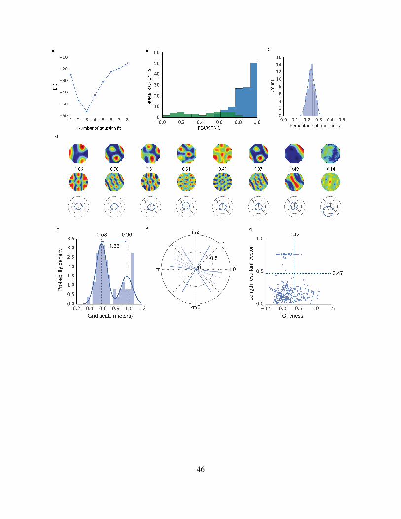
Figure 1: Entorhinal-like representations emerge in a network trained to path integrate. a,

Schematic of network architecture (see Extended Data Figure 1 for details) . b, Example trajectory

(15s), self-location decoded from place cells resembles actual path (respectively, dark and light-

blue). c, Accuracy of decoded location before (blue) and after (green) training. d, Linear layer

units exhibit spatially tuned responses resembling grid, border, and head direction cells. Ratemap

shows activity over location (top), spatial autocorrelogram of the ratemap with gridness indicated

(middle), polar plot show activity vs. head direction (bottom). e, Spatial scale of grid-like units

(n = 129) is clustered. Distribution is more discrete22 than chance (effect size = 2.98, 95% CI

[0.97, 4.91]) and best fit by a mixture of 3 Gaussians (centres 0.47, 0.70 & 1.06m, ratio=1.49 &

1.51). f, Directional tuning of the most strongly directional units (n = 52). Lines indicate length

and orientation of resultant vector (see Methods), exhibiting a six-fold clustering reminiscent of

conjunctive grid cells24. g, Distribution of gridness and directional tuning. Dashed lines indicate

95% confidence interval from null distributions (based on 500 data permutations), 14 (11%) grids

exhibit directional modulation (see Methods). Similar results were seen in a circular environment

(Extended Data Figure 3).

6

To ascertain how robust these representations were, we retrained the network 100 times,72

in each instance finding similar proportions of grid-like units (mean 23% SD 2.8%, units with73

significant gridness scores) and other spatially modulated units (Extended Data Figure 3). Con-74

versely, grid-like representations did not emerge in networks without regularization (e.g. dropout,75

see Methods; also see 25, Extended Data Figure 4). Therefore, the use of regularization, including76

dropout which has been viewed to be a parallel of noise in neural systems16, was critical to the77

emergence of entorhinal-like representations. Notably, therefore, our results show that grid-like78

representations reminiscent of those found in the mammalian entorhinal cortex emerge in a generic79

network trained to path integrate, contrasting with previous approaches using pre-configured grid80

cells (e.g. 26; see Supplemental Discussion). Further our results are consistent with the view that81

grid cells represent an efficient and robust basis for a location code updated by self-motion cues6–9.82

Next, we sought to test the hypothesis that the emergent representations provide an effective83

basis function for goal-directed navigation in complex, unfamiliar, and changeable environments,84

when trained through deep RL. Entorhinal grid cells have been proposed to provide a Euclidean85

spatial metric and thus support the calculation of goal-directed vectors, enabling animals to follow86

direct routes to a remembered goal, a process known as vector-based navigation7, 10, 11. Theoreti-87

cally, the advantage of decomposing spatial location into a multi-scale periodic code, as provided88

by grid cells, is that the relative position of two points can be retrieved by examining the differ-89

ence in the code at the level of each scale — combining the modulus remainders to return the90

true vector7, 11 (Fig. 2a). However, despite the obvious utility of such a framework, experimen-91

tal evidence for the direct involvement of grid representations in goal-directed navigation is still92

7

lacking.93

To develop an agent with the potential for vector-based navigation, we incorporated the “grid94

network” described above, into a larger architecture that was trained using deep RL (Fig. 2d,95

Extended Data Figure 5). As before, the grid network was trained using supervised learning but,96

to better approximate the information available to navigating mammals, it now received velocity97

signals perturbed with random noise as well as visual input. Experimental evidence suggests that98

place cell input to grid cells corrects for drift and anchors grids to environmental cues21. To parallel99

this, visual input was processed by a ”vision module” consisting of a convolutional network that100

produced place and head direction cell activity patterns which were provided as input to the grid101

network 5% of the time – akin to a moving animal making occasional, imperfect observations of102

salient environmental cues27 (see Methods, Fig. 2b&c and Extended Data Figure 5). The output103

of the linear layer of the grid network, corresponding to the agent’s current location, was provided104

as input to the “policy LSTM”, a second recurrent network controlling both the agent’s actions105

and outputting a value function. Additionally, whenever the agent reached the goal, the ”goal grid106

code” — activity in the linear layer — was subsequently provided to the policy LSTM during107

navigation as an additional input.108

We first examined the navigational capacities of the agent in a simple setting inspired by the109

classic Morris water maze (Fig. 2b&c; 2.5m×2.5m square arena; see Methods and Supplemental110

Results). Notably, the agent was still able to self localize accurately in this more challenging setting111

where ground truth information about location was not provided and velocity inputs were noisy112

8

(mean error after 15s trajectory, 12cm vs 88cm for an untrained network, effect size = 2.82; 95% CI113

[2.79, 2.84], Fig. 2e). Further, the agent exhibited proficient goal-finding abilities, typically taking114

direct routes to the goal from arbitrary starting locations (Fig. 2h). Performance exceeded that115

of a control place cell agent (Fig. 2f, Supplemental Results and Methods), chosen because place116

cells provide a robust representation of self-location but are not thought to provide a substrate117

for long range vector calculations11. We examined the units in the linear layer, again finding a118

heterogeneous population resembling those found in entorhinal cortex, including grid-like units119

(21.4%) as well as other spatial representations (Fig. 2g, Extended Data Figure 6) — paralleling120

the dependence of mammalian grid cells on self-motion information15, 28 and spatial cues6, 21.121

9

10

Figure 2: One-shot open field navigation to a hidden goal. a, Schematic of vector-based

navigation11. b, Overhead view of typical environment (icon indicates agent and facing direc-

tion). c, Agent view of (b). d, Schematic of Deep RL architecture (see Extended Data Figure 5) e,

Accuracy of self-location decoded from place cell units. f, Performance of grid cell agent and place

cell agent (y-axis shows reward obtained within a single episode, 10 points per goal arrival, gray

band displays the 68% confidence interval based on 5000 bootstrapped samples). g, As before the

linear layer develops spatial representations similar to entorhinal cortex. Left to right, 2 grid cells,

1 border cell, and 1 head direction cell. h, On the first trial of an episode the agent explores to find

the goal and subsequently navigates directly to it. i, After successful navigation, the policy LSTM

was supplied with a ”fake” goal grid-code, directing the agent to this location where no goal was

present. j&k, Decoding of goal-directed metric codes (i.e. Euclidean distance and direction) from

the policy LSTM of grid cell and place cell agents. The bootstrapped distribution (1000 samples)

of correlation coefficients are each displayed with a violin plot overlaid on a Tukey boxplot.

We next turn to our central claim, that grid cells endow agents with the ability to perform122

vector-based navigation, enabling downstream regions to calculate goal directed vectors by com-123

paring current activity with that of a remembered goal7, 10, 11. In the agent, we expect these calcu-124

lations to be performed by the policy LSTM, which receives the current activity pattern over the125

linear layer (termed “current grid code”; see Fig. 2d and Extended Data Figure 5) as well as that126

present the last time the agent reached the goal (termed “goal grid code”), using them to control127

movement. Hence we performed several manipulations, which yielded four lines of evidence in128

11

support of the vector-based navigation hypothesis (see Supplemental Results for details).129

First, to demonstrate that the goal grid code provided sufficient information to enable the130

agent to navigate to an arbitrary location, we substituted it with a ”fake” goal grid code sampled131

randomly from a location in the environment (see Methods). The agent followed a direct path to132

the newly specified location, circling the absent goal (Fig. 2i) — similar to rodents in probe trials133

of the Morris water maze (escape platform removed). Secondly, we demonstrated that withholding134

the goal grid code from the policy LSTM of the grid cell agent had a strikingly deleterious effect135

on performance (see Extended Data Fig. 6c). Thirdly, we demonstrated that the policy LSTM of136

the grid cell agent contained representations of key components of vector-based navigation (Figure137

2j&k), and that both Euclidean distance (difference in r = 0.17; 95% CI [0.11, 0.24]) and allocentric138

goal direction (difference in r = 0.22; 95% CI [0.18, 0.26]) were represented more strongly than in139

the place cell agent. Notably, a neural representation of goal distance has recently been reported140

in mammalian hippocampus29. Finally, we provide evidence consistent with a prediction of the141

vector-based navigation hypothesis, namely that a targeted lesion (i.e. silencing) to the most grid-142

like units within the goal grid code should have a greater adverse effect on performance and the143

representation of vector-based metrics (e.g. Euclidean distance) than a sham lesion (i.e silencing144

of non-grid units; average score for 100 episodes: 126.1 vs. 152.5, respectively; effect size = 0.38,145

95% CI [0.34, 0.42] see Supplemental Results).146

Having demonstrated the effectiveness of grid-like representations in optimizing one-shot147

goal learning in a simple square arena, we assessed the agent’s performance in complex, procedurally-148

12

generated multi-room environments, termed “goal-driven” and “goal-doors” (see Methods). No-149

tably, these environments are challenging for deep RL agents with external memory (see Extended150

Data Figure 7e,f,h&i and Supplemental Results). Again, the grid-cell agent exhibited high levels151

of performance, was strikingly robust across a range of network hyperparameters (see Extended152

Data Figure 7a,b&c), and reached the goal more frequently than either control agents or a human153

expert — a typical benchmark for the performance of deep RL agents in game playing scenarios2154

(Fig. 3e&f and see Supplemental Results). Further, when agents were tested, without retraining,155

in environments considerably larger than those seen previously, only the grid cell agent was able156

to generalise effectively (Fig. 3g&h and see Supplemental Results). Despite the complexity of the157

”goal-driven” environment, we could still decode the key metric codes from the grid agent policy158

LSTM with high accuracy during the initial period of navigation – with decoding accuracy sub-159

stantially higher in the grid cell agent than both the place cell and deep RL control agents (Figure160

3j&k and Supplemental Results, Extended Data Figures 8 and 9 for control agent architectures).161

13

14

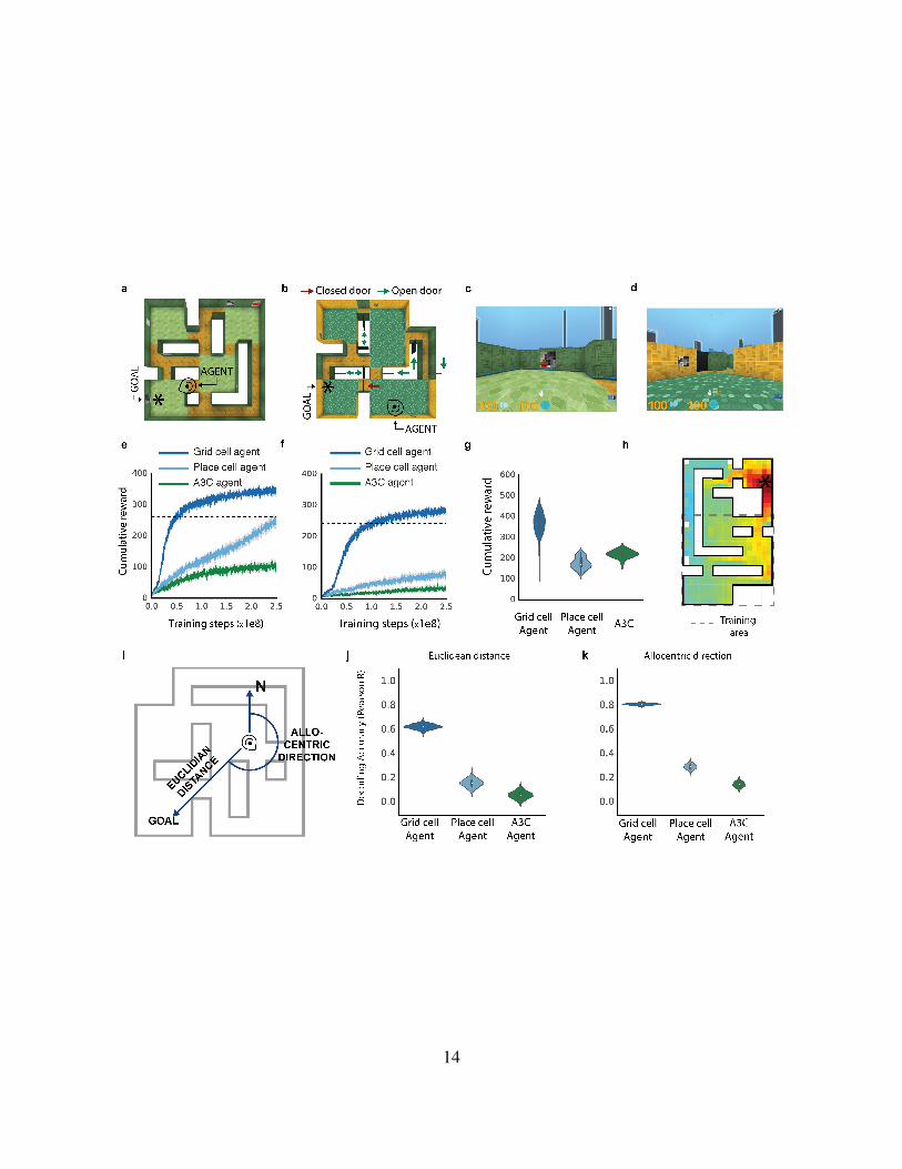
Figure 3: Navigation in complex environments a-b, Overhead view of multi-room environments

“goal-driven” (a) and “goal-doors” (i.e. with stochastic doors) (b) Goal (*) and agent locations

(head icon) are displayed. c-d, Agent views of (a) & (b) showing red goal and closed black door.

e-f, Agent training performance curves for (a) & (b), and performance of human expert (dotted

line). Performance is mean cumulative reward over 100 episodes. The gray band displays the 68%

confidence interval based on 5000 bootstrapped samples g, Distribution of test performance over

100 episodes, showing ability of agents to generalize to a larger version of goal-driven environ-

ment, displayed with a violin plot overlaid on a Tukey boxplot for each agent. h, The value function

of the grid cell agent is projected onto an example larger goal doors environment as a heatmap.

Dotted lines show the extent of the original training environment. Despite the larger size, the value

function clearly approximates Euclidean distance to goal. i, Schematic displaying the key metrics

required for vector-based navigation to a goal. j-k, Decoding of vector-based metric codes from

the policy LSTM of agents during navigation. The bootstrapped distribution (1000 samples) of

correlation coefficients are displayed with a violin plot overlaid on a Tukey boxplot in each case.162

15

Finally, a core feature of mammalian spatial behaviour is the ability to exploit novel short-163

cuts and traverse unvisited portions of space, a capacity thought to depend on vector-based164

navigation9, 11. Strikingly, the grid cell agent – but not comparison agents – robustly demonstrated165

these abilities in specifically designed neuroscience-inspired mazes, taking direct routes to the goal166

as soon as they became available (Fig. 4, Extended Data Figure 10 and Supplemental Results).167

16

17

Figure 4: Flexible use of short-cuts a, Example trajectory from grid cell agent during training in the linear

sunburst maze (only door 5 open; icon indicates start location). b, Testing configuration with all doors open:

grid cell agent uses the newly available shortcuts (100 episodes shown). c, Histogram showing agent’s

strong preference for most direct doors. d, Example grid cell agent trajectories (100) during training in the

double E-maze (corridor 1 doors closed). e, Testing configuration with corridor 1 open, and 100 grid agent

trajectories. f, Histogram analogous to panel c, agent prefers newely-available shortest route. See Extended

Data Figure 10 for performance of place cell agent.168

18

Conventional simultaneous localization and mapping (SLAM) techniques typically require169

an accurate and complete map to be built, with the nature and position of the goal externally170

defined30. In contrast, the deep reinforcement learning approach described in this work has the abil-171

ity to learn complex control policies end-to-end from a sparse reward, taking direct routes involving172

shortcuts to goals in an automatic fashion - abilities that exceed previous deep RL approaches3–5,173

and that would have to be hand-coded in any SLAM system.174

Our work, in demonstrating that grid-like representations provide an effective basis for flexi-175

ble navigation in complex novel environments, supports theoretical models of grid cells in vector-176

based navigation previously lacking strong empirical support7, 10, 11. We also show that vector-based177

navigation can be effectively combined with a path-based barrier avoidance strategy to enable the178

exploitation of optimal routes in complex multi-compartment environments. In sum, we argue that179

grid-like representations furnish agents with a Euclidean geometric framework — paralleling their180

proposed computational role in mammals as an early-developing Kantian-like spatial scaffold that181

serves to organize perceptual experience17, 18.182

183

1. LeCun, Y., Bengio, Y. & Hinton, G. Deep learning. Nature 521, 436–444 (2015).184

2. Silver, D. et al. Mastering the game of go with deep neural networks and tree search. Nature185

529, 484–489 (2016).186

3. Oh, J., Chockalingam, V., Singh, S. P. & Lee, H. Control of memory, active perception, and187

action in minecraft. In Proc. of International Conference on Machine Learning, ICML (2016).188

19

4. Kulkarni, T. D., Saeedi, A., Gautam, S. & Gershman, S. J. Deep successor reinforcement189

learning. CoRR abs/1606.02396 (2016). URL http://arxiv.org/abs/1606.02396.190

5. Mirowski, P. et al. Learning to navigate in complex environments. International Conference191

on Learning Representations (2017).192

6. Hafting, T., Fyhn, M., Molden, S., Moser, M.-B. & Moser, E. I. Microstructure of a spatial193

map in the entorhinal cortex. Nature 436, 801–806 (2005).194

7. Fiete, I. R., Burak, Y. & Brookings, T. What grid cells convey about rat location. Journal of195

Neuroscience 28, 6858–6871 (2008).196

8. Mathis, A., Herz, A. V. & Stemmler, M. Optimal population codes for space: grid cells197

outperform place cells. Neural Computation 24, 2280–2317 (2012).198

9. McNaughton, B. L., Battaglia, F. P., Jensen, O., Moser, E. I. & Moser, M.-B. Path integration199

and the neural basis of the’cognitive map’. Nature Reviews Neuroscience 7, 663–678 (2006).200

10. Erdem, U. M. & Hasselmo, M. A goal-directed spatial navigation model using forward trajec-201

tory planning based on grid cells. European Journal of Neuroscience 35, 916–931 (2012).202

11. Bush, D., Barry, C., Manson, D. & Burgess, N. Using grid cells for navigation. Neuron 87,203

507–520 (2015).204

12. Barry, C. & Burgess, N. Neural mechanisms of self-location. Current Biology 24, R330–R339205

(2014).206

20

13. Mittelstaedt, M.-L. & Mittelstaedt, H. Homing by path integration in a mammal. Naturwis-207

senschaften 67, 566–567 (1980).208

14. Bassett, J. P. & Taube, J. S. Neural correlates for angular head velocity in the rat dorsal209

tegmental nucleus. Journal of Neuroscience 21, 5740–5751 (2001).210

15. Kropff, E., Carmichael, J. E., Moser, M.-B. & Moser, E. I. Speed cells in the medial entorhinal211

cortex. Nature 523, 419–424 (2015).212

16. Srivastava, N., Hinton, G. E., Krizhevsky, A., Sutskever, I. & Salakhutdinov, R. Dropout: a213

simple way to prevent neural networks from overfitting. Journal of Machine Learning Re-214

search 15, 1929–1958 (2014).215

17. Wills, T. J., Cacucci, F., Burgess, N. & O’keefe, J. Development of the hippocampal cognitive216

map in preweanling rats. Science 328, 1573–1576 (2010).217

18. Langston, R. F. et al. Development of the spatial representation system in the rat. Science 328,218

1576–1580 (2010).219

19. Zhang, S.-J. et al. Optogenetic dissection of entorhinal-hippocampal functional connectivity.220

Science 340, 1232627 (2013).221

20. Sargolini, F. et al. Conjunctive representation of position, direction, and velocity in entorhinal222

cortex. Science 312, 758–762 (2006).223

21. Barry, C., Hayman, R., Burgess, N. & Jeffery, K. J. Experience-dependent rescaling of en-224

torhinal grids. Nature neuroscience 10, 682–684 (2007).225

21

22. Stensola, H. et al. The entorhinal grid map is discretized. Nature 492, 72–78 (2012).226

23. Stemmler, M., Mathis, A. & Herz, A. V. Connecting multiple spatial scales to decode the227

population activity of grid cells. Science advances 1, e1500816 (2015).228

24. Doeller, C. F., Barry, C. & Burgess, N. Evidence for grid cells in a human memory network.229

Nature 463, 657–661 (2010).230

25. Kanitscheider, I. & Fiete, I. Training recurrent networks to generate hypotheses about how the231

brain solves hard navigation problems. arXiv preprint arXiv:1609.09059 (2016).232

26. Milford, M. J. & Wyeth, G. F. Mapping a suburb with a single camera using a biologically233

inspired slam system. IEEE Transactions on Robotics 24, 1038–1053 (2008).234

27. Hardcastle, K., Ganguli, S. & Giocomo, L. M. Environmental boundaries as an error correction235

mechanism for grid cells. Neuron 86, 827–839 (2015).236

28. Chen, G., King, J. A., Burgess, N. & O’Keefe, J. How vision and movement combine in237

the hippocampal place code. Proceedings of the National Academy of Sciences 110, 378–383238

(2013).239

29. Sarel, A., Finkelstein, A., Las, L. & Ulanovsky, N. Vectorial representation of spatial goals in240

the hippocampus of bats. Science 355, 176–180 (2017).241

30. Dissanayake, M. G., Newman, P., Clark, S., Durrant-Whyte, H. F. & Csorba, M. A solution242

to the simultaneous localization and map building (slam) problem. IEEE Transactions on243

Robotics and Automation 17, 229–241 (2001).244

22

Methods245

Path integration: Supervised learning experiments.246

Simplified 2D environment. Simulated rat trajectories of duration T were generated in square247

and circular environments with walls of length L (diameter in the circular case). The simulated rat248

started at a uniformly sampled location and facing angle within the enclosure. A rat-like motion249

model31 was used to obtain trajectories that uniformly covered the whole environment by avoiding250

walls (see Table 1 in supplementary methods for the model’s parameters).251

Ground truth place cell distribution. Place cell activations, ~c ∈ [0, 1]N , for a given position252

~x ∈ R2, were simulated by the posterior probability of each component of a mixture of two-253

dimensional isotropic Gaussians,254

ci =e−‖~x−~µ(c)i ‖

2

2

2(σ(c))2

∑Nj=1 e

−‖~x−~µ(c)j ‖

2

2

2(σ(c))2

, (1)

where ~µ(c)i ∈ R2, the place cell centres, areN two-dimensional vectors chosen uniformly at random255

before training, and σ(c), the place cell scale, is a positive scalar fixed for each experiment.256

Ground truth head-direction cell distribution. Head-direction cell activations, ~h ∈ [0, 1]M , for257

a given facing angle ϕ were represented by the posterior probability of a each component of a258

mixture of Von Mises distributions with concentration parameter κ(h),259

hi =eκ(h) cos

(ϕ−µ(h)i

)∑M

j=1 eκ(h) cos

(ϕ−µ(h)j

) , (2)

23

where the M head direction centres µ(h)i ∈ [−π, π], are chosen uniformly at random before train-260

ing, and κ(h) the concentration parameter is a positive scalar fixed for each experiment.261

Supervised learning inputs. In the supervised setup the grid cell network receives, at each step t,262

the egocentric linear velocity vt ∈ R, and the sine and cosine of its angular velocity ϕ̇t.263

Grid cell network architecture The grid cell network architecture (Extended Data Figure 1)

consists of three layers: a recurrent layer, a linear layer, and an output layer. The single recurrent

layer is an LSTM (long short-term memory 32) that projects to place and head direction units via the

linear layer. The linear layer implements regularisation through dropout16. The recurrent LSTM

layer consists of one cell of 128 hidden units, with no peephole connections. Input to the recurrent

LSTM layer is the vector [vt, sin(ϕ̇t), cos(ϕ̇t)]. The initial cell state and hidden state of the LSTM,

~l0 and ~m0 respectively, are initialised by computing a linear transformation of the ground truth

place and head-direction cells at time 0:

~l0 = W (cp)~c0 +W (cd)~h0 (3)

~m0 = W (hp)~c0 +W (hd)~h0 (4)

The parameters of these two linear transformations (W (cp), W (cd), W (hp), and W (hd)) were opti-264

mised during training. The output of the LSTM, ~mt is then used to produce predictions of the place265

cells ~yt and head direction cells ~zt by means of a linear decoder network.266

The linear decoder consists of three sets of weights and biases: first, weights and biases that267

map from the LSTM hidden state ~mt to the linear layer activations ~gt ∈ R512. The other two268

sets of weights map from the linear layer activations ~gt to the predicted head directions, ~zt, and269

24

predicted place cells, ~yt, respectively via softmax functions33. Dropout 16 with drop probability 0.5270

was applied to each ~gt unit. Note that there is no intermediary non-linearity in the linear decoder.271

Supervised learning loss. The grid cell network is trained to predict the place and head-direction

cell ensemble activations, ~ct and ~ht respectively, at each time step t. During training, the network

was trained in a single environment where the place cell centres were constant throughout. The pa-

rameters of the grid cell network are trained by minimising the cross-entropy between the network

place cell predictions, ~y, and the synthetic place-cells targets, ~c, and the cross-entropy between

head-direction predictions, ~z, and their targets, ~h:

L(~y, ~z,~c,~h) = −N∑i=1

ci log(yi)−M∑j=1

hj log(zj), (5)

Gradients of (5) with respect to the network parameters were calculated using backpropagation272

through time34, unrolling the network into blocks of 100 time steps. The network parameters273

were updated using stochastic-gradient descent (RMSProp35), with weight decay36 for the weights274

incident upon the bottleneck activations. Hyperparameter values used for training are listed in275

Table 1.276

Gradient clipping In our simulations gradient clipping was used for parameters projecting from277

the dropout linear layer, gt, to the place and head-direction cell predictions ~yt and ~zt. Gradient278

clipping clips each element of the gradient vector to lie in a given interval [−gc, gc]. Gradient279

clipping is an important tool for optimisation in deep and recurrent artificial neural networks where280

it helps to prevent exploding gradients37. Gradient clipping also introduces distortions into the281

weight updates which help to avoid local minima38.282

25

Navigation through Deep RL283

Environments and Task We assessed the performance of agents on three environments seen by284

the agent from a first-person perspective in the DeepMind Lab 39 platform.285

Custom Environment: Square Arena This comprised a 10×10 square arena - which correspond286

to 2.5×2.5 meters assuming an agent speed of 15 cm/s (Fig. 2b, c). The arena contained a single,287

coloured, intra-arena cue whose position and colour changed each episode — as did the texture288

of the floor, the texture of the walls and the goal location. As in the goal-driven and goal-door289

environments described below, there were a set of distal cues (i.e. buildings) that paralleled the de-290

sign of virtual reality environments used in human experiments24. These distal cues were rendered291

at infinity — so as to provide directional but not distance information — and their configuration292

was consistent across episodes. At the start of each episode the agent (described below) started in293

a random location and was required to explore in order to find an unmarked goal, paralleling the294

task of rodents in the classic Morris water maze. The agent always started in the central 6×6 grids295

(i.e. 1.5×1.5 meters) of the environment. Noise in the velocity input ~ut was applied throughout296

training and testing (i.e. Gaussian noise ε, with µ = 0 and σ = 0.01). The action space is discrete297

(six actions) but affords fine-grained motor control (i.e. the agent could rotate in small increments,298

accelerate forward/backward/sideways, or effect rotational acceleration while moving).299

DeepMind Lab Environments: Goal-Driven and Goal-Doors Goal-driven and Goal-Doors are300

complex, visually-rich multi-room environments (see Fig. 3a-d). Mazes were formed within an301

11×11 grid, corresponding to 2.7 × 2.7 meters, (see below for definition of larger 11×17 mazes).302

26

Mazes were procedurally generated at the beginning of each episode; thus, the layout, wall textures,303

landmarks (i.e. intra-maze cues on walls) and goal location were different for each episode but304

consistent within an episode. Distal cues, in the form of buildings rendered at infinity, were as305

described for the square arena (see above).306

The critical difference between goal-driven and goal-doors tasks is that the latter had the307

additional challenge of stochastic doors within the maze. Specifically, the state of the doors (i.e.308

open or closed) randomly changed during an episode each time the agent reached the goal. This309

meant that the optimal path to the goal from a given location changed during an episode – requiring310

the agent to recompute trajectories.311

In both tasks the agent starts at a random location within the maze and its task is to explore312

to find the goal. The goal in both levels was always represented by the same object (see Fig. 3c).313

After getting to the goal the agent received a reward of 10 points after which it was teleported to314

a new random location within the maze. In both levels, episodes lasted a fixed duration of 5, 400315

environment steps (90 seconds).316

Generalisation on larger environments. We tested the ability of agents trained on the standard317

environment (11×11) to generalise to larger environments (11×17, corresponding to 2.7 × 4.25318

meters). The procedural generation and composition of these environments was done as with the319

standard environments. Each agent was trained in the 11×11 goal-driven maze for a total of 109320

environment steps, and the best performing replica (i.e. highest asymptotic performance averaged321

over 100 episodes in 11×11) was selected for evaluation in the larger maze. Note that the weights322

27

of the agent were frozen during evaluation on the larger maze. Evaluation was over 100 episodes323

of fixed duration 12, 600 environment steps (210 seconds).324

Probe mazes to assess shortcut behaviour To test the agent's ability to follow novel, goal-325

directed routes, we created a series of environments inspired by mazes designed to test the shortcut326

abilities of rodents.327

The first maze is a linearised version of Tolman's sunburst maze (Fig. 4a) used to determined328

if the agent was able to follow an accurate heading towards the goal when a path became available329

(see Supplementary Methods for details). In this maze, after reaching the goal, the agent was330

teleported to the original position with the same heading orientation. Here we tested agents trained331

in the “goal doors” environments. Specifically, the network weights were held frozen during testing332

and all the agents were tested for 100 episodes, each one lasting for a fixed duration of 5, 400333

environment steps (90 seconds).334

The second environment, the double E-maze (Fig. 4d), was designed to test the agent’s ability335

to traverse an entirely novel portion of space (see Supplementary Methods for details). In this maze336

we had a training and a testing condition. During the former agents were trained as in the other337

mazes (e.g. goal-driven; training details given below), whereas at test time weights were frozen.338

The agent always started in the central room (e.g. see Fig. 4d). The maze had stochastic doors339

with two different configurations, one for the training phase and one for testing phase. During340

training the state of the doors (i.e. open or closed) randomly changed during an episode each time341

the agent reached the goal. Critically, during training the corridors presenting the shortest route to342

28

the goal (i.e. the ones closer to the central room) were closed at both ends, preventing access or343

observation of the interior. At test time, after the agent reached the goal the first time, all doors344

were opened. All the agents were tested for 100 episodes, each one lasting for a fixed duration of345

5, 400 environment steps (90 seconds).346

Agent Architectures347

Architecture for the Grid Cell Agent. The agent architecture (see Extended Data Figure 5) was348

composed of a visual module, of the grid cell network (described above), and of an actor-critic349

learner40. The visual module was a neural network with input consisting of a three channel (RGB)350

64 × 64 image φ ∈ [−1, 1]3×84×84. The image was processed by a convolutional neural network351

(see Supplementary Methods for the details of the convolutional neural network), which produced352

embeddings, ~e, which in turn were used as input to a fully connected linear layer trained in a super-353

vised fashion to predict place and head-direction cell ensemble activations, ~c and ~h (as specified354

above), respectively. The predicted place and head direction cell activity patterns were provided355

as input to the grid network 5% of the time on average, akin to occasional imperfect observations356

made by behaving animals of salient environmental cues27. Specifically, the output of the convolu-357

tional network ~~e is then passed through a masking layer which zeroed the units with a probability358

of 95%.359

The grid cell network of the agent was implemented as in the supervised learning set up360

except that the LSTM (“GRID LSTM”) was not initialised based upon ground truth place cell361

activations but rather set to zero. The input to the grid cell network were the two translational362

29

velocities, u and v, as in DeepMind Lab it is possible to move in a direction different from the363

facing direction, and the sine and cosine of the angular velocity, ϕ̇, (these velocities are provided364

by DeepMind Lab) — and additionally the ~y and ~z output by the vision module. In contrast to the365

supervised learning case, here the grid cell network had to use ~y and ~z to learn how to reset its366

internal state each time it was teleported to an arbitrary location in the environment (e.g. after visit367

to goal). As in the supervised learning experiments described above, the configuration of place368

fields (i.e. location of place field centres in the 11×11 environments, “goal-driven” and “goal-369

doors”, 10×10 square arena, and 13×13 double E) were constant throughout training (i.e. across370

episodes).371

For the actor-critic learner the input was a three channel (RGB) 64 × 64 image φt ∈372

[−1, 1]3×84×84, which was processed by a convolutional neural network followed by a fully con-373

nected layer (see Supplementary Methods for the details of the convolutional neural network). The374

output of the fully connected layer of the convolutional network ~e1t was then concatenated with375

the reward rt, the previous action at−1, the current “grid code”, ~gt, goal “grid code”, ~g∗ (i.e.376

linear layer activations observed last time the goal was reached) — or zeros if the goal had not377

yet been reached in the episode. Note we refer to these linear layer activations as “grid codes”378

for brevity, even though units in this layer comprise also units resembling head direction cells, and379

border cells (e.g. see Extended Figure 6a). This concatenated input was provided to an LSTM with380

256 units. The LSTM had 2 different outputs. The first output, the actor, is a linear layer with 6381

units followed by a softmax activation function, that represents a categorical distribution over the382

agent’s next action. The second output, the critic, is a single linear unit that estimates the value383

30

function. Note that we refer to this as the ”policy LSTM” for brevity, even though it also outputs384

the value function.385

Comparison agents We compared the performance of the grid cell agent against two agents386

specifically because they use a different representational scheme for space (i.e. place cell agent,387

place cell prediction agent), and relate to theoretical models of goal-directed navigation from the388

neuroscience literature (e.g. 41, 42). We also compared the grid cell agent against a baseline deep389

RL agent, Asynchronous Advantage Actor-Critic (A3C)40.390

Place cell agent. The place cell agent architecture is shown in Extended Data Figure 8b. In con-391

trast to the grid cell agent, the place cell agent used ground truth information: specifically, the392

ground-truth place, ~ct, and head-direction, ~ht, cell activations (as described above). These activity393

vectors were provided as input to the policy LSTM in an analogous way to the provision of grid394

codes in the grid cell agent.395

Specifically, the output of the fully connected layer of the convolutional network ~et was396

concatenated with the reward rt, the previous action at−1, the ground-truth current place code,397

~ct, and current head-direction code, ~ht — together with the ground truth goal place code, ~c∗, and398

ground truth head direction code, ~h∗, observed last time the goal was reached — or zeros if the399

goal had not yet been reached in the episode (see Extended Data Figure 8b). The convolutional400

network had the same architecture described for the grid cell agent.401

Place cell prediction agent. The architecture of the place cell prediction agent (Extended Data402

Figure 9a) is similar to the grid cell agent described above: the key difference is the nature of the403

31

input provided to the policy LSTM as described below. The place cell prediction agent had a grid404

cell network — with the same parameters as that of the grid cell agent. However, instead of using405

grid codes from the linear layer of the grid network ~g, as input for the policy LSTM (i.e. as in406

the grid cell agent), we used the predicted place cell population activity vector ~y and the predicted407

head direction population activity vector ~z (i.e. the activations present on the output place and head408

direction unit layers of the grid cell network at each timestep) (see Supplementary Methods).409

The critical difference between the place cell agent and the place cell prediction agent (see410

Extended Data Figure 8b and 9a respectively) is that the former used ground truth information (i.e.411

place and head direction cell activations for current location and goal location) - whereas the latter412

used the population activity produced across the output place and head direction cell layers (i.e.413

for current location and goal location) by the linear layer of the same grid network as utilised by414

the grid cell agent.415

A3C We implemented the asynchronous advantage actor-critic architecture described in40 with416

convolutional network having the same architecture described for the grid cell agent (Extended417

Data Figure 8a).418

Other Agents We also assessed the performance of two deep RL agents with external mem-419

ory (Extended Data Figure 9b), which served to establish the challenging nature of the multi-420

compartment environments (goal-doors and goal-driven). First, we implemented a memory net-421

work agent (“NavMemNet”) consisting of the FRMQN architecture3 but instead of Q-learning we422

used the Asynchronous Advantage Actor-Critic (A3C) algorithm described below. Further, the423

32

input to memory was generated as an output from the LSTM controller (Extended Data Figure424

9b), rather than constituting embeddings from the convolutional network (i.e. as in3). The convo-425

lutional network had the same architecture described for the grid cell agent and the memory was426

formed of 2 banks (keys and values), each one with 1350 slots.427

Second, we implemented a Differentiable Neural Computer (“DNC”) agent which uses428

content-based retrieval and writes to the most recently used or least recently used memory slot.43429

Training algorithms We used the Asynchronous Advantage Actor-Critic (A3C) algorithm40,430

which implements a policy, π(a|s, θ), and an approximation to its value function, V (s, θ), using a431

neural network parameterised by θ. A3C adjusts the network parameters using n-step lookahead432

values, R̂t =∑

i=0...n−1 γirt+i + γnV (st+n, θ), to minimise: LA3C = Lπ + αLV + βLH, where433

Lπ = −Est∼π[R̂t

], LV = Est∼π

[(R̂t − V (st, θ)

)2], LH = −Est∼π [H(π(·|st, θ))]. Where LH is434

a policy entropy regularisation term (see Supplementary Methods for details of the reinforcement435

learning approach). The grid cell network and the vision module were trained with the same loss436

reported for supervised learning: L(~y, ~z,~c,~h) = −∑N

i=1 ci log(yi)−∑M

j=1 hj log(zj)437

Agent training details. We follow closely the approach of40. Each experiment used 32 actor-critic438

learner threads running on a single CPU machine. All threads applied updates to their gradients439

every 4 actions (i.e. action repeat of 4) using RMSProp with shared gradient statistics40. All the440

experiments were run for a total of 109 environment steps.441

In architectures where the grid cell network and the vision module were present we used442

a shared buffer 44, 45 where we stored the agents experiences at each time-step, et = (φt, ut, vt),443

33

collected over many episodes. All the 32 actor-critic workers were updating the same shared444

buffer which had a total size of 20e6 slots. The vision module was trained with mini batches of445

size 32 frames (~φ) sampled randomly from the replay buffer. The grid cell network was trained446

with mini batches of size 10, randomly sample from the buffer, each one comprising a sequence447

of 100 consecutive observations, [~φ, ~u,~v]. These mini batches were firstly forwarded through the448

vision module to get ~c, and ~h, which were then passed trough a masking layer which masked them449

to 0 with a probability of 95% (i.e. as described above in section on grid cell architecture). The450

output of this masking layer was then concatenate with ~u, ~v, ~sinϕ̇, ~cosϕ̇, which were then used451

as inputs to the grid network, as previously described (see Extended Data Figure 5 for details).452

Both networks were trained using one single thread, one to train the vision module and another to453

train the grid network (so in total we used 34 threads). Also, there was no gradient sharing between454

the actor-critic learners, the vision module and the grid network.455

The hyperparameters of the grid cell network were kept fixed across all the simulations and456

were derived from the best performing network in the supervised learning experiments. For the457

hyperparameter details of the vision module, the grid network and the actor-critic learner please458

refer to Table 2. For each of the agents in this paper, 60 replicas were run with hyperparameters459

sampled from the same interval (see Table 2) and different initial random seeds.460

Details for lesion experiment To conduct a lesioning experiment in the agent we trained the grid461

cell agent with dropout applied on the goal grid code input ~g∗. Specifically, every 100 training steps462

we generated a random mask to silence 20% of the units in the goal grid code (~g∗) - i.e. units were463

zeroed. This procedure was implemented to ensure that the policy LSTM would become robust464

34

through training to receiving a lesioned input (i.e. would not catastrophically fail), and still be able465

to perform the task.466

We then selected the agent with the best performance over 100 episodes, and we computed467

the grid score of all units found in ~g. The critical comparison to test the importance of grid-like468

units to vector-based navigation was as follows. In one condition we ran 100 testing episodes469

where we silenced the 25% units in ~g∗ with the highest grid scores. In the other condition, we ran470

100 testing episodes with the same agent with 25% random units in ~g∗ silenced. In this second case471

we ensured head direction cells with a resultant vector length of more than 0.47 were not silenced,472

to preserve crucial head direction signals. We then compared the performance, and representation473

of metrics relating to vector-based navigation, of the agents under these two conditions.474

Details of experiment using ”fake” goal grid code To demonstrate that the goal grid code pro-475

vided sufficient information to enable the agent to navigate to an arbitrary location we took an476

agent trained in the square arena, we froze the weights and we ran it in the same square arena for477

5, 400 steps. Critically, after the 6th time that the agent reach the goal, we sampled the grid code478

from a random point that the agent visited in the environment (called fake goal grid code). We479

then substituted the true goal grid code with this fake goal grid code, to show that this would be480

sufficient to direct the agent to a location where there was no actual goal.481

Agent Performance For evaluating agent performance during training (as in Fig. 2f, Fig. 3e,f)482

we selected the 30 replicas (out of 60) which had the highest average cumulative reward across483

100 episodes. Also we assessed the robustness of the architecture over different initial random484

35

seeds and the hyperparameters in Table 2 by calculating the area under the curve (AUC). To plot485

the AUC we ran 60 replicas with hyperparameters sampled from the same interval (see Table 2)486

and different initial random seeds (Extended Data Figure 7a-c).487

Neuroscience-based analyses of network units488

Generation of activity maps Spatial (ratemaps) and directional activity maps were calculated489

for individual units as follows. Each point in the trajectory was assigned to a specific spatial and490

directional bin based on its location and direction of facing. Spatial bins were defined as a 32×32491

square grid spanning each environment and directional bins as 20 equal width intervals. Then, for492

each unit, the mean activity over all the trajectories points assigned to that bin was found. These493

values were displayed and analysed further without additional smoothing.494

Inter-trial stability For each unit the reliability of spatial firing between baseline trials was as-495

sessed by calculating the spatial correlation between pairs of rate maps taken at 2 different logging496

steps in training (t = 2e5; t′ = 3e5). The total training time was 3e5 so the points were selected497

with enough time difference to minimise the chances of finding random correlations. The Pearson498

product moment correlation coefficient was calculated between equivalent bins in the two trials499

and unvisited bins were excluded from the measure.500

Quantification of spatial activity Where possible, we assessed the spatial modulation of units501

using measures adopted from the neuroscience literature. The hexagonal regularity and scale of502

grid-like patterns were quantified using the gridness score18, 20 and grid scale20, measures derived503

from the spatial autocorellogram20 of each unit’s ratemap. Similarly, the degree of directional504

36

modulation exhibited by each unit was assessed using the length of the resultant vector46 of the505

directional activity map. Finally, the propensity of units to fire along the boundaries of the envi-506

ronment was quantified with the border score47.507

The gridness and border scores exhibited by units in the linear layer were benchmarked508

against the 95th percentile of null distributions obtained using a permutation procedure (spatial509

field shuffle48) applied to each unit’s ratemap. This shuffling procedure aimed to preserve the lo-510

cal topography of fields within each ratemap while distributing the fields themselves at random48.511

The means, over units, of the thresholds obtained were gridness > 0.37 and border score > 0.50.512

Units exceeding these thresholds were considered to be grid-like and border-like, respectively. To513

identify directionally modulated cells we applied Rayleigh tests of directional uniformity to the514

binned directional activity maps. A unit was considered to be directionally modulated if the null515

hypothesis of uniform was rejected at the α = 0.01 level - corresponding to units with resultant516

vector length in excess of 0.47 (See Supplementary Methods for further details).517

Clustering of scale in grid-like units To determine if grid-like units exhibited a tendency to518

cluster around specific scales we applied two methods. First, following22, to determine if the scales519

of grid-like units (gridness > 0.37, 129/512 units) followed a continuous or discrete distribution520

we calculated the discreteness measure22 of the distribution of their scales (see Supplementary521

Methods). The discreteness score of the real data was found to exceed that of all of the 500 shuffles.522

Second, to characterise the number and location of scale clusters, the distribution of scales from523

grid-like units was fit with Gaussian mixture distributions, 3 components were found to provide the524

most parsimonious fit, indicating the presence of 3 scale clusters. (See Supplementary Methods525

37

for further details.)526

Multivariate decoding of representation of metric quantities within LSTM To test whether the527

grid agent learns to use the predicted vector based navigation (VBN) metric codes, we recorded the528

activation from the hidden units of the the Policy LSTM layer while the agent navigated 200 hun-529

dred episodes in the land maze. We used L2-regularized (ridge) regression to decode Euclidean530

distance and allocentric direction to the goal (see Supplementary Methods for full decoding de-531

tails). We specifically focussed on twelve steps (steps 9-21) during the early portion of navigation,532

but after the agent has had time to accurately self-localize. It is this early period after the agent has533

reached the goal for the first time where a VBN strategy should be most effective. We conducted534

the same analysis on the place cell agent control which is not predicted to use vector-based naviga-535

tion as efficiently. The decoding accuracy was measured as the correlation between predicted and536

actual metric values in held-out data. Decoding accuracy was compared across different agents by537

assessing the difference in decoding correlations between the agents. A bootstrap method (using538

10,000 samples) was used to computed a 95% confidence interval on this correlation difference,539

and these are reported for each comparison. The same approach was used to decode and compare540

these two metrics in the lesioned agents on the land maze. Finally, to explore VBN metrics in a541

more complex environment, the same method was applied to the goal-driven task. In this case we542

also investigated metric decoding in the control A3C agent.543

Data availability statement All reinforcement learning tasks described throughout the paper were544

built using the publicly available DeepMind Lab platform (https://github.com/deepmind/lab). We545

expect to release this set of tasks through this platform in the near future.546

38

Code availability statement We will release the code for the supervised learning experiments547

within the next six months. The codebase for the deep RL agents makes use of proprietary com-548

ponents, and we are unable to publicly release this code. However, all experiments and agents are549

described in sufficient detail to allow independent replication.550

551

31. Raudies, F. & Hasselmo, M. E. Modeling boundary vector cell firing given optic flow as a cue.552

PLoS computational biology 8, e1002553 (2012).553

32. Hochreiter, S. & Schmidhuber, J. Long short-term memory. Neural computation 9, 1735–1780554

(1997).555

33. Bridle, J. S. Training stochastic model recognition algorithms as networks can lead to max-556

imum mutual information estimation of parameters. In Touretzky, D. S. (ed.) Advances in557

Neural Information Processing Systems 2, 211–217 (Morgan-Kaufmann, 1990).558

34. Elman, J. L. & McClelland, J. L. Exploiting lawful variability in the speech wave. Invariance559

and variability in speech processes 1, 360–380 (1986).560

35. Tieleman, T. & Hinton, G. Lecture 6.5—RmsProp: Divide the gradient by a running average561

of its recent magnitude. COURSERA: Neural Networks for Machine Learning (2012).562

36. MacKay, D. J. A practical bayesian framework for backpropagation networks. Neural com-563

putation 4, 448–472 (1992).564

37. Pascanu, R., Mikolov, T. & Bengio, Y. On the difficulty of training recurrent neural networks.565

ICML (3) 28, 1310–1318 (2013).566

39

38. Ackley, D. H., Hinton, G. E. & Sejnowski, T. J. A learning algorithm for boltzmann machines.567

Cognitive science 9, 147–169 (1985).568

39. Beattie, C. et al. Deepmind lab. CoRR abs/1612.03801 (2016). URL http://arxiv.569

org/abs/1612.03801.570

40. Mnih, V. et al. Asynchronous methods for deep reinforcement learning. In Proceedings of the571

33nd International Conference on Machine Learning, ICML 2016, New York City, NY, USA,572

June 19-24, 2016, 1928–1937 (2016).573

41. Touretzky, D. S., Redish, A. D. et al. Theory of rodent navigation based on interacting repre-574

sentations of space. Hippocampus 6, 247–270 (1996).575

42. Foster, D., Morris, R., Dayan, P. et al. A model of hippocampally dependent navigation, using576

the temporal difference learning rule. Hippocampus 10, 1–16 (2000).577

43. Graves, A. et al. Hybrid computing using a neural network with dynamic external memory.578

Nature 538, 471–476 (2016).579

44. Mnih, V. et al. Human-level control through deep reinforcement learning. Nature 518, 529–580

533 (2015).581

45. Lin, L.-J. Reinforcement learning for robots using neural networks. Tech. Rep., Carnegie-582

Mellon Univ Pittsburgh PA School of Computer Science (1993).583

46. Knight, R. et al. Weighted cue integration in the rodent head direction system. Philosophical584

Transactions of the Royal Society of London B: Biological Sciences 369, 20120512 (2014).585

40

47. Solstad, T., Boccara, C. N., Kropff, E., Moser, M.-B. & Moser, E. I. Representation of geo-586

metric borders in the entorhinal cortex. Science 322, 1865–1868 (2008).587

48. Barry, C. & Burgess, N. To be a grid cell: Shuffling procedures for determining gridness.588

BiorXiv (2017).589

There is Supplemental Information that contains additional results, discussion and details590

about the Methods.591

Acknowledgements We thank Max Jaderberg, Volodymyr Mnih, Adam Santoro, Tom Schaul, Kim592

Stachenfeld and Jason Yosinski for discussions; Matthew Botvinick, and Jane Wang for comments on an593

earlier version of the manuscript . C.Ba. funded by Royal Society and Wellcome Trust.594

Competing Interests The authors declare that they have no competing financial interests.595

Correspondence Correspondence and requests for materials should be addressed to Andrea Ban-596

ino, Caswell Barry, Dharshan Kumaran (email: abanino@google.com, caswell.barry@ucl.ac.uk, dku-597

maran@google.com).598

Author Contributions Conceived project. A.B, D.K., C.Ba., R.H., P.M., B.U., Contributed ideas to ex-599

periments. A.B., D.K., C.Ba., B.U., R.H., T.L., C.Bl., P.M., A.P., T.D., J.M., K.K., N.R., G.W., R.G., D.H.,600

R.P. Performed experiments and analysis: A.B., C.Ba., B.U., M.C., T.L., H.S., A.P., B.Z, F.V. Development601

of testing platform and environments. C.Be., S.P., R.H., T.L., G.W., D.K., A.B., B.U., D.H. Human expert602

tester. A.S. Managed project. D.K, R.H., A.B., H.K., S.G., D.H. Wrote paper. D.K., A.B., C.Ba., T.L.,603

C.Bl., B.U., M.C., A.P., R.H., N.R., K.K., D.H.604

41

Extended data for Vector-based Navigation using Grid-like Representations in Artificial Agents.605

42

Extended Data Figure 1: Network architecture in the supervised learning experiment. The recurrent

layer of the grid cell network is an LSTM with 128 hidden units. The recurrent layer receives as input the

vector [vt, sin(ϕ̇t), cos(ϕ̇t)]. The initial cell state and hidden state of the LSTM, ~l0 and ~m0 respectively, are

initialised by computing a linear transformation of the ground truth place ~c0 and head-direction ~h0 activity

at time 0. The output of the LSTM is followed by a linear layer on which dropout is applied. The output of

the linear layer, ~gt, is linearly transformed and passed to two softmax functions that calculate the predicted

head direction cell activity, ~zt, and place cell activity, ~yt, respectively. We found evidence of grid-like and

head direction-like units in the linear layer activations ~gt.

43

44

Extended Data Figure 2: Linear layer spatial activity maps from the supervised learning ex-

periment. Spatial activity plots for all 512 units in the linear layer ~gt. Units exhibit spatial activity

patterns resembling grid cells, border cells, and place cells — head direction tuning was also

present but is not shown.606

45

46

Extended Data Figure 3: Characterization of grid-like units in Square environment and Circular

environment. a) The scale (assessed from the spatial autocorrelogram of the ratemaps) of grid-like units

exhibited a tendency to cluster at specific values. The number of distinct scale clusters was assessed by

sequentially fitting Gaussian mixture models with 1 to 8 components. In each case, the efficiency of the

fit (likelihood vs. number of parameters) was assessed using Bayesian information criterion (BIC). BIC

was minimized with three Gaussian components indicating the presence of three distinct scale clusters. b)

Spatial stability of units in the linear layer of the supervised network was assessed using spatial correlations

— bin-wise Pearson product moment correlation between spatial activity maps (32 spatial bins in each

map) generated at 2 different points in training, t = 2e5 and t′ = 3e5 training steps. That is, 23 of the

way through training and the end of training, respectively. This separation was imposed to minimise the

effect of temporal correlations and to provide a conservative test of stability. Grid-like units (gridness >

0.37) blue, directionally modulated units (resultant vector length > 0.47) green. Grid-like units exhibit

high spatial stability, while directionally modulated units do not. c) Robustness of the grid representation to

starting conditions. The network was retrained 100 times with the same hyperparamters but different random

seeds controling the initialisation of network weights, ~c and ~h. Populations of grid-like units (gridness >

0.37) were found to appear in all cases, the average proportion of grid-like units being 23% (SD of 2.8%).

d) circular environment: the supervised network was also trained in a circular environment (diameter =

2.2m). As before, units in the linear layer exhibited spatially tuned responses resembling grid, border, and

head direction cells. Eight units are shown. Top, ratemap displaying activity binned over location. Middle,

spatial autocorrelogram of the ratemap, gridness20 is indicated above. Bottom, polar plot of activity binned

over head direction. e) Spatial scale of grid-like units (n = 56 (21.9%)) is clustered. Distribution is best fit

by a mixture of 2 Gaussians (centres 0.58 & 0.96m, ratio = 1.66). f) Distribution of directional tuning for 31

most directionally active units, single line for each unit indicates length and orientation of resultant vector46

g) Distribution of gridness and directional tuning. Dashed lines indicate 95% confidence interval derived

from shuffling procedure (500 permutations), 5 grid units (9%) exhibit significant directional modulation.607

47

48

Extended Data Figure 4: Grid-like units did not emerge in the linear layer when dropout was

not applied. Linear layer spatial activity maps (n=512) generated from a supervised network

trained without dropout. The maps do not exhibit the regular periodic structure diagnostic of grid

cells.608

49

50

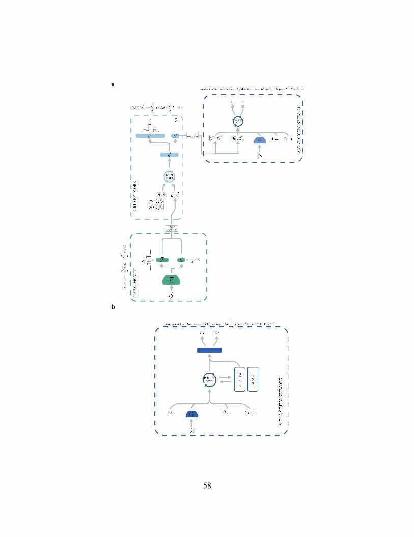
Extended Data Figure 5: Architecture of the grid cell agent. The architecture of the supervised

network (grid network, light blue dashed) was incorporated into a larger deep RL network, includ-

ing a visual module (green dashed) and an actor critic learner (based on A3C 40; dark blue dashed).

In this case the supervised learner does not receive the ground truth ~c0 and ~h0 to signal its initial

position, but uses input from the visual module to self-localize after placement at a random posi-

tion within the environment. Visual module: since experimental evidence suggests that place cell

input to grid cells functions to correct for drift and anchor grids to environmental cues21, 27, visual

input was processed by a convolutional network to produce place cell (and head direction cell)

activity patterns which were used as input to the grid network. The output of the vision module

was only provided 5% of the time to the grid network; see Methods for implementational details),

akin to occasional observations made by behaving animals of salient environmental cues27. The

output of the vision module was concatenated with ~u, ~v, ~sinϕ̇, ~cosϕ̇ to form the input to the

GRID LSTM, which is the same network as in the supervised case (see Methods and Extended

Data Figure 1). The actor critic learner (light blue dashed) receives as input the concatenation of

~e1t produced by a convolutional network with the reward rt, the previous action at − 1 , the linear

layer activations of the grid cell network ~gt (“current grid-code”), and the linear layer activations

observed last time the goal was reached, ~g∗. ~g∗ (“goal grid-code”), which is set to zeros if the goal

has not been reached in the episode. The fully connected layer was followed by an LSTM with

256 units. The LSTM has 2 different outputs. The first output, the actor, is a linear layer with 6

units followed by a softmax activation function, that represents a categorical distribution over the

agent’s next action ~πt. The second output, the critic, is a single linear unit that estimates the value

function vt.609

51

52

Extended Data Figure 6: Characterisation of grid-like representations and robustness of per-

formance for the grid cell agent in the square “land maze” environment. a) Spatial activity

plots for the 256 linear layer units in the agent exhibit spatial patterns similar to grid, border, and

place cells. b) Cumulative reward indexing goal visits per episode (goal = 10 points) when distal

cues are removed (dark blue) and when distal cues are present (light blue) — performance is un-

affected, hence dark blue largely obscures light blue. Average of 50% best agent replicas (n=32)

plotted (see Methods). The gray band displays the 68% confidence interval based on 5000 boot-

strapped samples. c) Cumulative reward per episode when no goal code was provide (light blue)

and when goal code was provided (dark blue). When no goal code was provided the agent perfor-

mance fell to that of the baseline deep RL agent (A3C) (100 episodes average score ”no goal code”

= 123.22 vs. A3C = 112.06 ,effect size = 0.21, 95% CI [0.18, 0.28]). Average of 50% best agent

replicas (n=32) plotted (see Methods). The gray band displays the 68% confidence interval based

on 5000 bootstrapped samples. d) After locating the goal for the first time during an episode the

agent typically returned directly to it from each new starting position, showing decreased latencies

for subsequent visits, paralleling the behaviour exhibited by rodents.610

53

54

Extended Data Figure 7: Robustness of grid cell agent and performance of other agents. a-

c) AUC performance gives the robustness to hyperparameters (i.e. learning rate, baseline cost,

entropy cost - see Table 2 in Supplementary Methods for details of the range) and seeds (see

Methods). For each environment we run 60 agent replicas (see Methods). Light purple is the

grid agent, blue is the place cell agent and dark purple is A3C. a) Square arena b) Goal-driven

c) Goal Doors. In all cases the grid cell agent shows higher robustness to variations in hyper-

parameters and seeds. d-i Performance of place cell prediction/NavMemNet/DNC agents (see

Methods) against grid cell agent. Dark blue is the grid cell agent (Extended Data Figure 5), green

is the place cell prediction agent (Extended Data Figure 9a), purple is the DNC agent, light blue

is the NavMemNet agent (Extended Data Figure 9b). The gray band displays the 68% confidence

interval based on 5000 bootstrapped samples. d-f) Performance in goal-driven. g-i) Performance

in goal-doors. Note that the performance of the place cell agent (Extended Data Figure 8b, lower

panel) is shown in Figure 3.611

55

56

Extended Data Figure 8: Architecture of the A3C and place cell agent. a) The A3C implemen-

tation is as described in40. b) The place cell agent was provided with the ground-truth place, ~ct,

and head-direction, ~ht, cell activations (as described above) at each time step. The output of the

fully connected layer of the convolutional network ~et was concatenated with the reward rt, the

previous action at − 1, the ground-truth current place code, ~ct, and current head-direction code, ~ht

— together with the ground truth goal place code, ~c∗, and ground truth head direction code, ~h∗,

observed the last time the agent reached the goal (see Methods).612

57

58

Extended Data Figure 9: Architecture of the place cell prediction agent and of the NavMem-

Net agent. a) The architecture of the place cell prediction agent is similar to the grid cell agent

— having a grid cell network with the same parameters as that of the grid cell agent. The key

difference is the nature of the input provided to the policy LSTM. Instead of using grid codes from

the linear layer of the grid network ~g, we used the predicted place cell population activity vector

~y and the predicted head direction population activity vector ~z (i.e. the activations present on the

output place and head direction unit layers of the grid cell network, corresponding to the current

and goal position) as input for the policy LSTM. As in the grid cell agent, the output of the fully

connected layer of the convolutional network, ~et, the reward rt, and the previous action at−1, were

also input to the policy LSTM. The convolutional network had the same architecture described for

the grid cell agent. b) NavMemNet agent. The architecture implemented is the one described in3,

specifically FRMQN but the Asynchronous Advantage Actor-Critic (A3C) algorithm was used in

place of Q-learning. The convolutional network had the same architecture described for the grid

cell agent and the memory was formed of 2 banks (keys and values), each one composed of 1350

slots.613

59

60

Extended Data Figure 10: Flexible use of short-cuts a) Overhead view of the linear sunburst maze in

initial configuration, with only door 5 open. Example trajectory from grid cell agent during training (green

line, icon indicates start location). b) Test configuration with all doors open: grid cell agent uses the newly

available shortcuts (multiple episodes shown). c) Histogram showing proportion of times the agent uses

each of the doors during 100 test episodes. The agent shows a clear preference for the shortest paths. d)

Performance of grid cell agent and comparison agents during test episodes. e) Example grid cell agent and

f) example place cell agent trajectory during training in the double E-maze (corridor 1 doors closed). g-h) in

the test phase, with all doors open, the grid cell agent exploits the available shortcut (g), while the place cell

agent does not (h). i-j) Performance of agents during training (i) and test (j). k-l, The proportion of times

the grid (k) and place (l) cell agents use the doors on the 1st to 3rd corridor during test. The grid cell agent

shows a clear preference for available shortcuts, while the place cell agent does not.614

61

Supplemental Information for Vector-based Navigation using Grid-like Representations in615

Artificial Agents.616

Andrea Banino1∗, Caswell Barry2∗, Benigno Uria1, Charles Blundell1, Timothy Lillicrap1, Piotr617

Mirowski1, Alexander Pritzel1, Martin Chadwick1, Thomas Degris1, Joseph Modayil1, Greg618

Wayne1, Hubert Soyer1, Fabio Viola1, Brian Zhang1, Ross Goroshin1, Neil Rabinowitz1, Razvan619

Pascanu1, Charlie Beattie1, Stig Petersen1, Amir Sadik1, Stephen Gaffney1, Helen King1, Koray620

Kavukcuoglu1, Demis Hassabis1, Raia Hadsell1, Dharshan Kumaran1621

1DeepMind, 5 New Street Square, London EC4A 3TW, UK.622

2Department of Cell and Developmental Biology, University College London, London, UK623

∗equal contribution.624

62

This section contains:625

1. Supplementary Results626

(a) Assessing path integration and goal-finding in a square arena627

(b) Experimental manipulations to test the Vector-Based navigation hypothesis628

(c) Comparison of grid cell agent with other agents in complex, procedurally-generated629

multi-room environments630

(d) Probe mazes assessing ability to take novel shortcuts631

2. Supplementary Discussion632

(a) Backpropagation through time (BPTT)633

(b) Relationship to previous models of grid cells634

3. Supplementary Methods635

(a) Navigation through Deep RL636

(b) Additional information about Agent Architectures637

(c) Training algorithms638

(d) Neuroscience-based analyses of units639

(e) Multivariate decoding of representation of metric quantities within LSTM640

(f) Statistical reporting641

63

1 - Supplementary Results for Vector-based Navigation using Grid-like Representations in Ar-642

tificial Agents.643

1a - Assessing path integration and goal-finding in a square arena To better understand the644

advantage conveyed by a grid-like representation, we trained the agent to navigate to an unmarked645

goal in a simple setting inspired by the classic Morris water maze (Fig. 2b&c; 2.5m×2.5m square646

arena; see Methods). The agent was trained in episodes to ensure it was able to generalize to647

arbitrary open field enclosures, each episode consisted of 5, 400 steps — corresponding to ap-648

proximately 90 s in total — after which the goal location, floor texture, and cue location were649

randomized. An episode started with the agent in a random location, requiring it to first explore650

in order to find an unmarked goal. Upon reaching the goal the agent was teleported to another651

random location and continued to navigate with the aim of maximising the number of times it652

reached the goal before the episode ended. In this setting self-localisation was more challenging.653

Previously, in experiment described above, information about the ground truth initial location was654

provided to initialise the LSTM, here the grid network learned to use visual information to de-655

termine the agent’s starting location and to correct for drift resulting from noise introduced to the656

velocity inputs (see Methods). Despite these differences the grid network continued to self-localize657

accurately, outputting place cell predictions consistent with the agent’s location (Fig. 2e).658

After locating the goal for the first time during an episode, the agent typically returned directly to it659

from each new starting position, showing decreased latencies for subsequent visits (average score660

for 100 episodes: grid cell agent = 289 vs place cell agent = 238, effect size = 1.80, 95% CI [1.63,661

1.99], Fig. 2h, Extended Data Figure 6d). Performance of the grid cell agent was substantially662

64

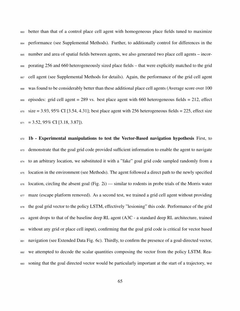
better than that of a control place cell agent with homogeneous place fields tuned to maximize663

performance (see Supplemental Methods). Further, to additionally control for differences in the664

number and area of spatial fields between agents, we also generated two place cell agents – incor-665

porating 256 and 660 heterogeneously sized place fields – that were explicitly matched to the grid666

cell agent (see Supplemental Methods for details). Again, the performance of the grid cell agent667

was found to be considerably better than these additional place cell agents (Average score over 100668

episodes: grid cell agent = 289 vs. best place agent with 660 heterogeneous fields = 212, effect669

size = 3.93, 95% CI [3.54, 4.31]; best place agent with 256 heterogeneous fields = 225, effect size670

= 3.52, 95% CI [3.18, 3.87]).671

1b - Experimental manipulations to test the Vector-Based navigation hypothesis First, to672

demonstrate that the goal grid code provided sufficient information to enable the agent to navigate673

to an arbitrary location, we substituted it with a ”fake” goal grid code sampled randomly from a674

location in the environment (see Methods). The agent followed a direct path to the newly specified675

location, circling the absent goal (Fig. 2i) — similar to rodents in probe trials of the Morris water676

maze (escape platform removed). As a second test, we trained a grid cell agent without providing677

the goal grid vector to the policy LSTM, effectively ”lesioning” this code. Performance of the grid678

agent drops to that of the baseline deep RL agent (A3C - a standard deep RL architecture, trained679

without any grid or place cell input), confirming that the goal grid code is critical for vector based680

navigation (see Extended Data Fig. 6c). Thirdly, to confirm the presence of a goal-directed vector,681

we attempted to decode the scalar quantities composing the vector from the policy LSTM. Rea-682

soning that the goal directed vector would be particularly important at the start of a trajectory, we683

65

focused on the initial portion of navigation after the agent had reached the goal and was teleported684

to a new location. We found that the policy LSTM of the grid cell agent contained representations685

of two key components of vector-based navigation (Euclidean distance, and allocentric goal direc-686

tion), and that both were more strongly present than in the place cell agent (Euclidean distance687

difference in r = 0.17; 95% CI [0.11, 0.24]; Goal direction difference in r = 0.22; 95% CI [0.18,688

0.26]; Figure 2j&k). Notably, a neural representation of goal distance has recently been reported689

in mammalian hippocampus29 (also see 49). To determine the behavioral relevance of these two690

metric codes, we examined the goal-homing accuracy in each episode over several steps immedi-691

ately following the period of metric decoding. We found that variation in both Euclidean distance692

(r = 0.22, 95% CI [-0.32, -0.09]) and allocentric goal direction (r = 0.22, 95% CI [-0.38, -0.15])693

decoding error correlated with subsequent behavioral accuracy. This suggests that stronger metric694

codes are indeed important for accurate goal-homing behavior.695

Finally, to determine the specific contribution of the grid-like units, we made targeted lesions to the696

goal grid code and reexamined performance and representation of the goal directed vector. When697

25% of the most grid-like units were silenced (see Methods), performance was worse than lesion-698

ing 25% at random (average score for 100 episodes: 126.1 vs. 152.5, respectively; effect size =699

0.38, 95% CI [0.34, 0.42]). Further, as expected, goal-directed vector codes were more strongly700

degraded (Euclidean distance: random lesions decoding accuracy r = 0.45, top-grid lesions de-701

coding accuracy r = 0.38, difference in decoding accuracy = 0.08, 95% CI [0.03, 0.13]). We also702

performed an additional experiment where the effect of the targeted grid lesion was compared to703

that of lesioning non-grid units with patchy firing (see Supplemental Methods - section 3d for the704

66

details of the procedure). Our results show that the targeted grid cell lesion had a greater effect705

than the patchy non-grid cell lesion (average score for 100 episodes: 126.1 vs. 151.7, respectively;706

effect size = 0.38, 95% CI [0.34, 0.42]). These results support a role for the grid-like units in707

vector-based navigation, with the relatively mild impact on performance potentially accounted for708

by the difference in lesioning networks as compared to animals. Specifically, the procedure for709

lesioning networks differs in important respects from experimental lesions in animals — which710

bears upon the results observed. Briefly, networks have to be trained in the presence of an in-711

complete goal grid code and thus have the opportunity to develop a degree of robustness to the712

lesioning procedure – which would otherwise likely result in a catastrophic performance drop (see713

Methods). This opportunity is not typically afforded to experimental animals. This, therefore, may714

explain the significant but relatively small performance deficit observed in lesioned networks.715

1c - Comparison of grid cell agent with other agents in challenging, procedurally-generated716

multi-room environments Our comparison agents for the grid cell agent included an agent specif-717

ically designed to use a different representational scheme for space (i.e. place cell agent, see Ex-718

tended Data Figure 8b and see Methods), and a baseline deep RL agent (A3C 40, see Extended Data719

Figure 8a). The place cell agent relates to theoretical models of goal-directed navigation from the720

neuroscience literature (e.g.41, 42). A key difference between grid and place cell based models is721

that the former are proposed to enable the computation of goal-directed vectors across large-scale722

spaces7, 10, 11and50, whereas place cell based models are inherently limited in terms of navigational723

range (i.e. to the largest place field) and do not support route planning across unexplored spaces11.724

First, we test these three agents in the “goal-driven” maze (see Methods). The grid-cell agent ex-725

67

hibited high levels of performance, and over the course of 100 episodes, attained an average score726

of 346.5 (video: https://youtu.be/BWqZwLQfwlM), beating both the place cell agent (average727

score 258.76; contrast effect size = 1.98, 95% CI [1.79, 2.18]) and the A3C agent (average score728

137.00; contrast effect size = 14.31, 95% CI [12.91, 15.71]). The grid cell agent showed markedly729

superior performance compared to the other agents in the “goal-doors” maze (average score over730

100 episodes: grid cell agent = 284.30 vs place cell agent = 90.53, effect size = 7.86, 95% CI731

[7.09, 8.63]; A3C agent = 48.69, effect size = 7.73, 95% CI [6.97, 8.48]) (video of grid cell agent:732

https://youtu.be/BWqZwLQfwlM). Interestingly, therefore, the enhanced performance of the grid733

cell agent was particularly evident when it was necessary to recompute trajectories due to changes734

in the door configuration, highlighting the flexibility of vector-based navigation in exploiting ad735

hoc short-cuts (Fig. 3f).736

The grid cell agent exhibited stronger performance than a professional human player in both “goal-737

driven” (average score: grid cell agent = 346.50 vs. professional human player = 261, effect size738

= 4.00, 95% CI [3.50, 4.52]) and “goal-doors” (average score: grid cell agent = 284.30 vs. profes-739

sional human player = 240.5, effect size = 2.49, 95% CI [2.18, 2.81]). The human expert received740

10 episodes worth of training in each environment before undergoing 20 episodes of testing. This741

is considerably less training than that experienced by the network. Importantly, however, the mam-742

malian brain has evolved to path integrate and naturally the human expert had a lifetimes worth of743

relevant navigational experience. Hence, although directly drawing concrete conclusions from rel-744

ative performance of human and agents is necessarily difficult, providing human-level performance745

is useful as a broad comparison and represents a commonly used benchmark in similar papers44.746

68

We also tested the ability of agents trained on the standard environment (11× 11) to generalise to747

larger environments (11 × 17, corresponding to 2.7 × 4.25 meters) (see Methods). The grid cell748

agent exhibited strong generalistion performance compared to the control agents (average score749

over 100 episodes grid cell agent = 366.5 vs place cell agent = 175.7, effect size = 4.60, 95% CI750

[4.16, 5.06]; A3C agent = 219.4, effect size = 3.78, 95% CI [3.41, 4.15]).751

We assessed the performance of two deep RL agents with external memory3,43 (see Extended Data752

Figure 9b). Whilst these agents were trained purely using RL — that is, they did not utilize super-753

vised learning implemented by the grid cell agent — their relatively poor performance illustrates754

the challenge posed by the environments used (i.e. goal-driven and goal-doors) and shows that is755

not readily solved by the use of external memory alone. Importantly, this also serves to highlight756

the substantial advantage afforded to agents that can exploit vector-based mechanisms grounded757

in a grid-cell based Euclidean framework of space — and the potential for future work to examine758

the combination of such navigational strategies with more memory-intensive approaches. We also759

compare the grid cell agent with a variation of the place cell agent which used the predicted place760

cell and head direction cell as input to the Policy LSTM instead of the ground truth information761

(see Extended Data Figure 9a and Supplementary Methods). This agent exhibited substantially762

poorer performance than the grid agent.763

Further, decoding accuracy was substantially and significantly higher in the grid cell agent than764

both the place cell (Euclidean distance difference in r = 0.44; 95% CI [0.37, 0.51]; Goal direction765

difference in r = 0.52; 95% CI [0.49, 0.56]) and deep RL (Euclidean distance difference in r =766

0.57; 95% CI [0.5, 0.63]; Goal direction difference in r = 0.66; 95% CI [0.62, 0.70]) control agents767

69

(Figure 3j&k).768

1d - Probe mazes assessing ability to take novel shortcuts A core feature of mammalian spatial769

behaviour is the ability to exploit novel shortcuts and traverse unvisited portions of space9, a capac-770

ity thought to depend on vector-based navigation9, 11. To assess this, we examined the ability of the771

grid cell agent and comparison agents to use novel shortcuts when they became available in specif-772

ically configured probe mazes (see Methods for details). First, agents trained in the goal-doors773

environment were exposed to a linearized version of Tolman’s sunburst maze. The grid cell agent,774

but not comparison agents, was reliably able to exploit shortcuts, preferentially passing through775

the doorways that offered a direct route towards the goal (Fig. 4a-c, and Extended Data Figure 10).776

The average testing score of the grid cell agent was higher than that of the place agent (124.1 vs777

60.9, effect size = 1.46, 95% CI [1.32, 1.61]) and of the A3C agent (124.1 vs. 59.7, effect size =778

1.51, 95% CI [1.36, 1.66]).779

Next, to test the agents’ abilities to traverse a previously unvisited section of an environment,780

we employed the “double-E shortcut” maze (Fig. 4d-f, and Extended Data Figure 10e-l). During781

training, the corridor presenting the shortest route to the goal was closed at both ends, preventing782

access or observation of the interior. In this simple configuration the grid and place cell agents783

performed similarly, exceeding the RL control agent (Extended Data Figure 10i). However, at test,784

when the doors were opened, the grid cell agent was able to exploit the short-cut corridor, whereas785

the control agents continued to follow the longer route they had previously learnt (Extended Data786

Figure 10j-l). In the “double-E shortcut” maze performance does not significantly differ between787

the grid and place cell agents, but both are significantly better than the A3C control (grid cell788

70

agent vs. place cell agent, effect size = 0.27, 95% CI [0.24, 0.29]; grid cell agent vs. A3C agent,789

effect size = 2.99, 95% CI [2.69, 3.29]; place cell agent vs. A3C agent, effect size = 2.92, 95%790

CI [2.63, 3.21]). When shortcuts become available in the test phase, the grid cell agent performs791

significantly better than the place agent (grid cell agent vs. place cell agent, effect size = 1.89, 95%792

CI [1.69, 2.09]; grid cell agent vs. A3C agent, effect size = 12.77, 95% CI [11.48, 14.07]; place793

cell agent vs. A3C agent, effect size = 14.87, 95% CI [13.35, 16.38]).794

2 - Supplementary Discussion for Vector-based Navigation using Grid-like Representations in795

Artificial Agents.796

2a - Backpropagation through time (BPTT) Whilst backpropagation provides a powerful mech-797

anism for adjusting the weights within hierarchical networks analogous to those found in the brain798

(e.g. the ventral visual stream), it has long been thought to be biologically implausible for several799

reasons: for example, it requires access to information that is non-local to a synapse (i.e. informa-800

tion about errors many layers downstream). However, recent research in several directions have801

provided fresh new insights into how a process akin to backpropagation may be implemented in802

the brain 51. Whilst less research has been conducted into how BPTT could be implemented in the803

brain, recent work points to potentially promising avenues that deserve further exploration 52.804

2b - Relationship to previous models of grid cells Our work contrasts with previous approaches805

where grid cells have been hard-wired53–56and57, derived through eigendecomposition of place806

fields58, 59, or arisen through self organization in the absence of an objective function60. It is worth807

noting that our experiments were not designed to provide insights into the development of grid808

71

cells in the brain — due to the limitations of the training algorithm used (i.e. backpropagation) in809

terms of biological plausibiliy (although see 61). More generally, however, our findings accord with810

the perspective that the internal representations of individual brain regions such as the entorhinal811

cortex arise as a consequence of optimizing for specific ethologically important objective functions812

(e.g. path integration) — providing a parallel to the optimization process in neural networks62.813

72

3 - Supplementary Methods for Vector-based Navigation using Grid-like Representations in814

Artificial Agents.815

3a - Navigation through Deep RL816

Probe mazes to test for shortcut behavior The first maze used to test shortcut behaviour was a817

linearized version of Tolman's sunburst maze63 (Fig. 4a). The maze was used to determined if the818

agent was able to follow an accurate heading towards the goal when a path became available. The819

maze was size 13×13 and contained 5 evenly spaced corridors, each of which had a door at the820

end closest to the start position of the agent. The agent always started on one side of the corridors821

with the same heading orientation (North; see Fig 4a) and the goal was always placed in the same822

location on the other side of the corridors. Until the agent reached the goal the first time only one823

door was open (door 5, Fig. 4a), but after that all the doors were opened for the remainder of the824

episode. After reaching the goal, the agent was teleported to the original position with the same825

heading orientation. This maze was used to test the shortcut capabilities of agents that had been826

previously trained in the ”goal doors” environment. All the agents were tested in the maze for 100827

episodes, each one lasting for a fixed duration of 5, 400 environment steps (90 seconds).828

The second maze, termed double E-maze, was designed to test the agents abilities to traverse829

a previously unvisited section of an environment. The maze was size 12×13 and was formed830

of 2 symmetric sides each one with 3 corridors. The goal location was always on the bottom831

right or left, and the location was randomized over episodes. During training, the left and right832

corridors closest to the bottom (i.e. those providing the shortest paths to the goals) were always833

73

closed from both sides to avoid any exploration down these corridors (see Extended Data Figure834

10e&f). This ensured any subsequent shortcut behavior had to traverse unexplored space. Of the835

remaining corridors, at any time, on each side only one was accessible (top or middle, randomly836

determined). Each time the agent reached the goal, the doors were randomly configured again837

(with the same constraints). The agent always started in a random location in the central room838

with a random orientation. At test time, after the agent reached the goal for the first time, all839

corridors were opened, allowing potential shortcut behavior (see Extended Data Figure 10g&h).840

During the test phase, the agent always started in the center of the central room facing north. Each841

agent was trained for 1e9 environment step divided into episodes of 5, 400 steps (90 seconds), and842

subsequently tested for 100 episodes, each one lasting for a fixed duration of 5, 400 environment843

steps (90 seconds).844

3b - Additional information about Agent Architectures845

Details of vision module in the grid cell agent The convolutional neural network had four con-846

volutional layers. The first convolutional layer had 16 filters of size 5×5 with stride 2 and padding847

2. The second convolutional layer had 32 filters of size 5 × 5 with stride 2 and padding 2. The848

third convolutional layer had 64 filters of size 5× 5 with stride 2 and padding 2. Finally, the fourth849

convolutional layer with 128 filters of size 5 × 5 with stride 2 and padding 2. All convolutional850

hidden layers were followed by a rectifier nonlinearity. The last convolution was followed by a851

fully connected layer with 256 hidden units. The same convolutional neural network was used for852

the actor-critic learner. The weights of the two network were not shared.853

74

Further details about the place cell agent Place cell agent with homogeneously sized place854

fields: we tested agents with fields — modelled as regular 2D Gaussians — having standard devi-855

ations of 7.5cm, 25cm, and 75cm bins. The agent with fields of size 7.5cm was found to perform856

best (highest cumulative reward on the Morris water maze task; see Supplemental Results) and857

hence was chosen as the primary place cell control agent (see main text for score comparisons).858

Place cell agent with heterogeneously sized place fields: to control for differences in the num-859

ber and area of spatial fields between agents, we also generated two further place cell agents that860

were explicitly matched to the grid cell agent. Specifically, we used a watershedding algorithm64861

to detect 660 individual grid fields in the grid-like units of the grid cell agent. The distribution862

of the areas of these fields were found to exhibit 3 peaks — based on a Gaussian fitting proce-863

dure — having means equivalent to 2D Gaussians with standard deviations of 8.2cm, 15.0cm, and864

21.7cm. Hence we generated a further control agent having 395 place cells of size 8.2cm, 198865

of size 15.0cm, and 67 of 21.7cm — 660 place cells in total, the relative numbers reflecting the866

magnitudes of the Gaussians fit to the distribution. A final control agent was also generated having867

256 place cell units in total — the same number of linear layer units as the grid agent — distributed868

across the same three scales in a similar ratio. Additionally, we note that from a machine learn-869

ing perspective, the place cell and grid cell agents with the same number of linear layer units are870

in principle well matched since they are provided with the same input information and have an871

identical number of parameters.872

Place cell prediction agent. The architecture of the place cell prediction agent (Extended Data873

Figure 9a) is similar to the grid cell agent described in the Methods : the key difference is the874

75

nature of the input provided to the policy LSTM as described below. Specifically, the output of the875

fully connected layer of the convolutional network, ~et, was concatenated with the reward rt, the876

previous action at− 1, the current predicted place cell activity vector, ~yt, and the current predicted877

head direction cell activity vector ~ht — and the goal predicted place cell activity vector , ~y∗, and878

goal head direction activity vector, ~h∗, observed the last time the agent had reached the goal — or879

zeros if the agent had not yet reached the goal within the episode. The convolutional network had880

the same architecture described for the grid cell agent.881

3c - Training algorithms882

We assume the standard reinforcement learning setting where an agent interacts with an environ-883

ment over a number of discrete time steps. As previously defined the at time t the agent receives884

an observation ot along with a reward rt and produces an action at. The agent’s state st is a func-885

tion of its experience up until time t, st = f(o1, r1, a1, ..., ot, rt) (The specifics of ot are defined886

in the architecture section). The n-step return Rt:t+n at time t is defined as the discounted sum of887

rewards, R̂t =∑

i=0...n−1 γirt+i + γnV (st+n, θ). The value function is the expected return from888

state s, V π(s) = E[Rt:∞|st = s, π], under actions selected accorded to a policy π(a|s). See main889

methods for the details of the loss functions.890

3d - Neuroscience-based analyses of units891

Gridness score and grid scale calculation Following 20 and 18 spatial autocorrelograms of892

ratemaps were used to assess the gridness and grid scale of linear layer units. First, for each unit,893

the spatial autocorrelogram was calculated as defined in 20. To calculate gridness20, a measure894

76

of hexagonal periodicity, we followed the ’expanding gridness’ method introduced by 18. Briefly,895

a circular annulus centred on the origin of the autocorrelogram was defined, having radius of 8896

bins and with the central peak excluded. The annulus was rotated in 30◦ increments and, at each897

increment, the Pearson product moment correlation coefficient with the unrotated version of itself898

found. An interim gridness value was then defined as the highest correlation obtained from ro-899

tations of 30, 90 and 150◦ subtracted from the lowest at 0, 60 and 120◦. This process was then900

repeated, each time expanding the annuls by 2, up to a maximum of 20. Finally, the gridness value901

was taken as the highest interim score.902

Grid scale20, a simple measure of the wavelength of spatial periodicity, was defined from the903

autocorrelogram as follows. The six local maxima closest to but excluding the central peak were904

identified. Grid scale was then calculated as the median distance of these peaks from the origin.905

Directional measures Following46 the degree of directional modulation exhibited by each unit906

was assessed using the length of the resultant vector of the directional activity map. Vectors corre-907

sponding to each bin of the activity map were created:908

ri =

βi cosαi

βi sinαi

, (6)

where α and β are, respectively, the centre and intensity of angular bin i in the activity map. These

vectors were averaged to generate a mean resultant vector:

~r =

∑Nn=1 ri∑Nn=1 βi

, (7)

and the length of the resultant vector calculated as the magnitude of ~r. We used 20 angular bins.909

77

Border score To identify units that were preferentially active adjacent to the edges of the enclo-

sure we adopted a modified version of the border score47. For each of the four walls in the square

enclosure, the average activation for that wall, bi, was compared to the average centre activity c

obtaining a border score for that wall, and the maximum was used as the border-score for the unit:

bs = maxi∈{1,2,3,4}

bi − cbi + c

(8)

where bi is the mean activation for bins within db distance from the i-th wall and c the average910

activity for bins further than db bins from any wall. In all our experiments 20 by 20 bins where911

used and db took value 3.912

Threshold setting for gridness, border score, and directional measures The hexagonality of913

the spatial activity map (gridness), directional modulation (length of resultant vector), and propen-914

sity to be active against environmental boundaries (border scale) exhibited by units in the linear915

layer were benchmarked against null distributions obtained using permutation procedures6548.916

For the gridness measure and border score, null distributions were constructed using a ’field917

shuffle’ procedure equivalent to that specified by48. Briefly, a watershedding algorithm64 was ap-918

plied to the ratemap to segment spatial fields. The peak bin of each field was found and allocated919

to a random position within the ratemap. Bins around each peak were then incrementally replaced,920

retaining as far as possible their proximity to the peak bin. This procedure was repeated 100 times921

for each of the units present in the linear layer and the gridness and border score of the shuffled922

ratemaps assessed as before. In each case the 95th percentile of the resulting null distribution was923

found and used as a threshold to determine if that unit exhibited significant grid or border-like924

78

activity.925

To validate the thresholds obtained using shuffling procedures we calculated alternative null926

distributions by analysing the grid and border responses of linear units from 500 untrained net-927

works. Again, in each case, a grid score and border score for each unit was calculated, these were928

pooled, and the 95th percentile found. In all cases the thresholds obtained by the first method were929

found to be most stringent and these were used for all subsequent analyses930

To establish a significance threshold for directional modulation we calculated the length of931

the resultant vector that would demonstrate statistically significance under a Rayleigh test of direc-932

tional uniformity at α = 0.01. The resultant vector was calculated by first calculating the average933

activation for 20 directional bins. A threshold length of 0.47 for the resultant vector was obtained.934

The most stringent of these two thresholds was used.935

Clustering of scale in grid-like units To determine if grid-like units exhibited a tendency to936

cluster around specific scales we applied two methods.937

First, following 22, to determine if the scales of grid-like units (gridness > 0.37, 129/512938

units) followed a continuous or discrete distribution we calculated the ’discreteness measure’22939

of the distribution of their scales. Specifically, scales were binned into a histogram with 13 bins940

distributed evenly across a range corresponding to scales 10 to 36 spatial bins. ’Discreteness’941

was defined as the standard deviation of the counts in each bin. Again following22, statistical942

significance for this value was obtained by comparing it to a null distribution generated from a943

shuffled version of the same data. Specifically, shuffles were generated as follows: For each unit, a944

79

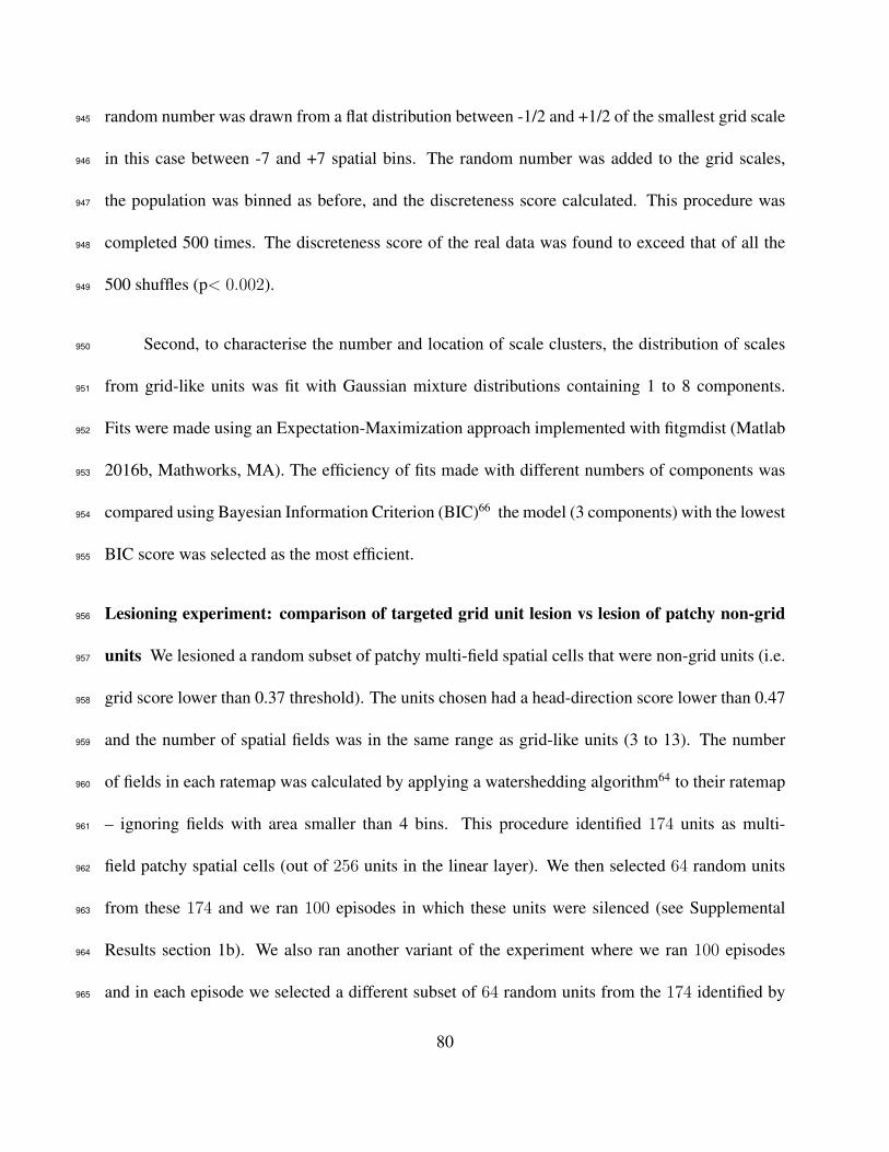
random number was drawn from a flat distribution between -1/2 and +1/2 of the smallest grid scale945

in this case between -7 and +7 spatial bins. The random number was added to the grid scales,946

the population was binned as before, and the discreteness score calculated. This procedure was947

completed 500 times. The discreteness score of the real data was found to exceed that of all the948

500 shuffles (p< 0.002).949

Second, to characterise the number and location of scale clusters, the distribution of scales950

from grid-like units was fit with Gaussian mixture distributions containing 1 to 8 components.951

Fits were made using an Expectation-Maximization approach implemented with fitgmdist (Matlab952

2016b, Mathworks, MA). The efficiency of fits made with different numbers of components was953

compared using Bayesian Information Criterion (BIC)66 the model (3 components) with the lowest954

BIC score was selected as the most efficient.955

Lesioning experiment: comparison of targeted grid unit lesion vs lesion of patchy non-grid956

units We lesioned a random subset of patchy multi-field spatial cells that were non-grid units (i.e.957

grid score lower than 0.37 threshold). The units chosen had a head-direction score lower than 0.47958

and the number of spatial fields was in the same range as grid-like units (3 to 13). The number959

of fields in each ratemap was calculated by applying a watershedding algorithm64 to their ratemap960

– ignoring fields with area smaller than 4 bins. This procedure identified 174 units as multi-961

field patchy spatial cells (out of 256 units in the linear layer). We then selected 64 random units962

from these 174 and we ran 100 episodes in which these units were silenced (see Supplemental963

Results section 1b). We also ran another variant of the experiment where we ran 100 episodes964

and in each episode we selected a different subset of 64 random units from the 174 identified by965

80

the watershedding procedure, and these units were silenced. The results were not qualitatively966

different from the former experiment (data not shown).967

3e - Multivariate decoding of representation of metric quantities within LSTM968

A key prediction of the vector-based navigation hypothesis is that grid codes should allow down-969

stream regions to compute a set of metric codes relevant to accurate goal-directed navigation.970

Specifically, Euclidean distance and allocentric direction to the goal should both be computed by971

an agent using vector-based navigation (see Fig. 2j&k also 3i-k). To test whether the same rep-972

resentations can be found in the grid cell agent, and thereby provide additional evidence that it is973

indeed using a vector-based navigation strategy, we recorded the activity in the policy LSTM of974

the grid cell agent while it navigated in the land-maze and goal-driven environments. For each en-975

vironment and agent, we collected data from 200 separate episodes. In each episode, we recorded976

data from the time period following the first time the agent reached the goal and was teleported to977

a new location in the maze. After an initial period to allow self-localization (8 steps), we exam-978

ined the representation of the metric quantities over the next 12 steps, where the LSTM activity979

was sampled at 4 even points over those steps. We focussed on this time period because the agent980

potentially has knowledge of the goal location, but has not yet been able to learn the optimal path981

to the goal. Thus it is this initial period of time where the computation of the vector-based naviga-982

tion metrics should be most useful, as this allows accurate navigation right from the start of being983

teleported to a new location. In the land maze task, we additionally collected the same data from a984

place cell agent control, and the two lesioned grid cell agents. In the goal driven task, we collected985

data from the place cell agent and A3C. For each agent, we applied a decoding analysis to the986

81

LSTM dictating the policy and value function. We ran two separate decoding analyses, looking987

for evidence of each of the two metric codes (i.e. Euclidean distance, allocentric goal direction).988

For each decoding analysis we trained a L2-regularized (ridge) regression model on all data apart989

from the first 21 time-steps of each episode. The model was then tested on the four early sampling990

steps of interest, where accuracy was assessed as the Pearson correlation between the predicted991

and actual values over the 200 episodes. The penalization parameter was selected by randomly992

splitting the training data into internal training and validation sets (90% and 10% of the episodes993

respectively). The optimal parameter was selected from 30 values, evenly spaced on a log scale994

between 0.001 and 1000, based on the best performance on the validation set. This parameter was995

then used to train the model on the full training set, and evaluated on the fully independent test set.996

As the allocentric direction metric is circular, we decomposed the vector into two target variables:997

the cosine and sine of the polar angle. All reported allocentric decoding results are the average998

of the cosine and sine results. For the purpose of comparing decoding accuracy across agents,999

we report the difference in accuracy, along with a 95% bootstrapped confidence interval on this1000

difference, based on 10,000 samples.1001

3f - Statistical reporting1002

We followed the guidelines outlined by67. Specifically reporting effect sizes and confidence in-

tervals. Unless otherwise stated, the effect sizes are calculated using the following formula:

effect size =µgroup1 − µgroup2

σpooled, (9)

82

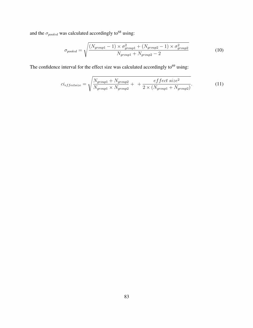
and the σpooled was calculated accordingly to68 using:

σpooled =

√(Ngroup1 − 1)× σ2

group1 + (Ngroup2 − 1)× σ2group2

Ngroup1 +Ngroup2 − 2(10)

The confidence interval for the effect size was calculated accordingly to69 using:

cieffectsize =

√Ngroup1 +Ngroup2

Ngroup1 ×Ngroup2

+ +effect size2

2× (Ngroup1 +Ngroup2). (11)

83

Parameter name Value Description

T 15 Duration of simulated trajectories (seconds)

L 2.2 Width and height of environment, or diameter for circular environment (meters)

d 0.03 Perimeter region distance to walls (meters)

σ(v) 0.13 Forward velocity Rayleigh distribution scale (m/sec)

µ(φ) 0 Rotation velocity Gaussian distribution mean (deg/sec)

σ(φ) 330 Rotation velocity Gaussian distribution standard deviation (deg/sec)

ρRH 0.25 Velocity reduction factor when located in the perimeter

∆RH 90 Change in angle when located in the perimeter (deg)

∆t 0.02 Simulation-step time increment (seconds)

N 256 Number of place cells

σ(c) 0.01 Place cell standard deviation parameter (meters)

M 12 Number of target head direction cells

κ(h) 20 Head direction concentration parameter

gc 10−5 Gradient clipping threshold

minibatch size 10 Number of trajectories used in the calculation of a stochastic gradient

trajectory length 100 Number of time steps in the trajectories used for the supervised learning task

learning rate 10−5 Step size multiplier in the RMSProp algorithm

momentum 0.9 Momentum parameter of the RMSProp algorithm

L2 regularisation 10−5 Regularisation parameter for linear layer

parameter updates 300000 Total number of gradient descent steps taken

Table 1: Supervised learning hyperparameters.

84

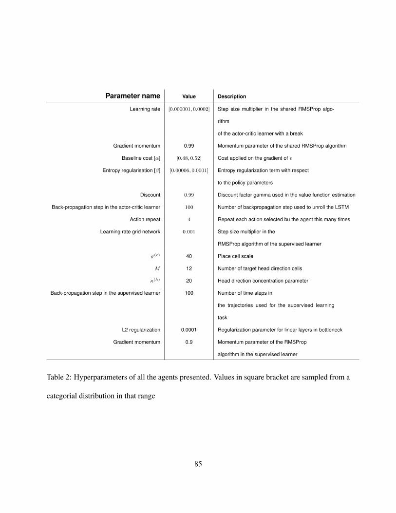
Parameter name Value Description

Learning rate [0.000001, 0.0002] Step size multiplier in the shared RMSProp algo-

rithm

of the actor-critic learner with a break

Gradient momentum 0.99 Momentum parameter of the shared RMSProp algorithm

Baseline cost [α] [0.48, 0.52] Cost applied on the gradient of v

Entropy regularisation [β] [0.00006, 0.0001] Entropy regularization term with respect

to the policy parameters

Discount 0.99 Discount factor gamma used in the value function estimation

Back-propagation step in the actor-critic learner 100 Number of backpropagation step used to unroll the LSTM

Action repeat 4 Repeat each action selected bu the agent this many times

Learning rate grid network 0.001 Step size multiplier in the

RMSProp algorithm of the supervised learner

σ(c) 40 Place cell scale

M 12 Number of target head direction cells

κ(h) 20 Head direction concentration parameter

Back-propagation step in the supervised learner 100 Number of time steps in

the trajectories used for the supervised learning

task

L2 regularization 0.0001 Regularization parameter for linear layers in bottleneck

Gradient momentum 0.9 Momentum parameter of the RMSProp

algorithm in the supervised learner

Table 2: Hyperparameters of all the agents presented. Values in square bracket are sampled from a

categorial distribution in that range

85

1003

49. Chadwick, M. J., Jolly, A. E., Amos, D. P., Hassabis, D. & Spiers, H. J. A goal direction signal1004

in the human entorhinal/subicular region. Current Biology 25, 87–92 (2015).1005

50. Kubie, J. L. & Fenton, A. A. Linear look-ahead in conjunctive cells: an entorhinal mechanism1006

for vector-based navigation. Frontiers in neural circuits 6, 20 (2012).1007

51. Scellier, B. & Bengio, Y. Towards a biologically plausible backprop. arXiv preprint1008

arXiv:1602.05179 914 (2016).1009

52. Ke, N. R. et al. Sparse attentive backtracking: Long-range credit assignment in recurrent1010

networks. arXiv preprint arXiv:1711.02326 (2017).1011

53. Burgess, N., Barry, C. & O’keefe, J. An oscillatory interference model of grid cell firing.1012

Hippocampus 17, 801–812 (2007).1013

54. Hasselmo, M. E., Giocomo, L. M. & Zilli, E. A. Grid cell firing may arise from interference1014

of theta frequency membrane potential oscillations in single neurons. Hippocampus 17, 1252–1015

1271 (2007).1016

55. Burak, Y. & Fiete, I. R. Accurate path integration in continuous attractor network models of1017

grid cells. PLoS Comput Biol 5, e1000291 (2009).1018

56. Fuhs, M. C. & Touretzky, D. S. A spin glass model of path integration in rat medial entorhinal1019

cortex. Journal of Neuroscience 26, 4266–4276 (2006).1020

86

57. Gustafson, N. J. & Daw, N. D. Grid cells, place cells, and geodesic generalization for spatial1021

reinforcement learning. PLoS Comput Biol 7, e1002235 (2011).1022

58. Stachenfeld, K. L., Botvinick, M. & Gershman, S. J. Design principles of the hippocampal1023

cognitive map. In Advances in neural information processing systems, 2528–2536 (2014).1024

59. Dordek, Y., Soudry, D., Meir, R. & Derdikman, D. Extracting grid cell characteristics from1025

place cell inputs using non-negative principal component analysis. eLife 5, e10094 (2016).1026

60. Widloski, J. & Fiete, I. How does the brain solve the computational problems of spatial1027

navigation? In Space, Time and Memory in the Hippocampal Formation, 373–407 (Springer,1028

2014).1029

61. Bengio, Y., Lee, D.-H., Bornschein, J., Mesnard, T. & Lin, Z. Towards biologically plausible1030

deep learning. arXiv preprint arXiv:1502.04156 (2015).1031

62. Marblestone, A. H., Wayne, G. & Kording, K. P. Toward an integration of deep learning and1032

neuroscience. Frontiers in Computational Neuroscience 10 (2016).1033

63. Tolman, E. C. et al. Cognitive maps in rats and men (1948).1034

64. Beucher, S. Use of watersheds in contour detection. In Proceedings of the International1035

Workshop on Image Processing (CCETT, 1979).1036

65. Yartsev, M. M., Witter, M. P. & Ulanovsky, N. Grid cells without theta oscillations in the1037

entorhinal cortex of bats. Nature 479, 103–107 (2011).1038

66. Schwarz, G. Estimating the dimension of a model. The Annals of Statistics 6, 461–464 (1978).1039

87

67. Halsey, L. G., Curran-Everett, D., Vowler, S. L. & Drummond, G. B. The fickle p value1040

generates irreproducible results. Nature methods 12, 179 (2015).1041

68. Olejnik, S. & Algina, J. Measures of effect size for comparative studies: Applications, inter-1042

pretations, and limitations. Contemporary educational psychology 25, 241–286 (2000).1043

69. Hedges, L. & Olkin, I. Statistical Methods for Meta-analysis (Academic Press, 1985). URL1044

https://books.google.co.uk/books?id=brNpAAAAMAAJ.1045

88