vector and tensor algebra - springer978-3-7643-7383-2/1.pdf · appendix a vector and tensor algebra...
TRANSCRIPT
Appendix A
Vector and Tensor Algebra
A.1 Vector Space. Basis
A real vector space is an algebraic structure consisting of a set V endowed withtwo operations. One of them is an internal operation denoted by + and satisfyingthe following properties:
i) Associativity.a + (b + c) = (a + b) + c ∀ a, b, c.
ii) Existence of a neutral element 0 such that
a + 0 = 0 + a = a ∀ a.
iii) Existence of a symmetric element : for each a there exists b such that
a + b = b + a = 0.
iv) Commutativity.a + b = b + a ∀ a, b.
Thus, V with the + operation is a commutative group.
The second operation is an external one, the product by real numbers, satis-fying the following properties:
v) λ(a + b) = λa + λb.
vi) λ(µa) = (λµ)a.
vii) (λ + µ)a = λa + µa.

162 Appendix A. Vector and Tensor Algebra
viii) 1a = a.
Elements of V are called vectors.
A set of vectors eiNi=1 is said to be
• linearly independent if
N∑i=1
λiei = 0 ⇒ λi = 0 ∀i ∈ 1, . . . , N, (A.1)
• a system of generators if
∀v ∈ V ∃λi, i = 1, . . . , N, such that v =N∑
i=1
λiei, (A.2)
• a basis if it is both linearly independent and a system of generators.
If B = e1, . . . , eN is a basis of V , then each v ∈ V can be written as alinear combination,
v =N∑
i=1
viei,
in a unique way. The vi ∈ R, i = 1, . . . , N, are called coordinates of v with respectto basis B.
Let us consider two bases in V , eiNi=1 and EiN
i=1. In particular, vectorsEi can be written as linear combinations of vectors eiN
i=1, namely,
El =N∑
i=1
Cliei. (A.3)
Now, let v be any vector in V . Let us denote by vei and vE
i , i = 1, . . . , N , thecoordinates of v with respect to basis eiN
i=1 and EiNi=1, respectively. If we
denote by ve the column vector of the former and by vE the column vector of thelatter, it is easy to see that
vE = [C]ve, (A.4)
where [C] is the matrix [C]ij = Cij with Cij given in (A.3).
A.2. Inner Product 163
A.2 Inner Product
A mapping ϕ : V × V −→ R is called an inner product if the following propertieshold:
1) ϕ is bilinear :
1.1) ϕ(λ1v1 + λ2v2,w) = λ1ϕ(v1,w) + λ2ϕ(v2,w),
1.2) ϕ(v, λ1w1 + λ2w2,w) = λ1ϕ(v,w1) + λ2ϕ(v,w2).
2) ϕ is symmetric:
ϕ(v,w) = ϕ(w,v).
3) ϕ is positive definite:
ϕ(v,v) > 0 ∀ v = 0.
Finite dimensional vector spaces with an inner product are called Euclideanvector spaces. For them we can define a norm by
|v| = ϕ(v,v)12 .
In what follows we write v · w instead of ϕ(v,w).
Two vectors v and w are said to be orthogonal if v ·w = 0.
A basis B = e1, . . . , eN is said to be orthogonal if ei · ej = 0 ∀ i = j andis said to be orthonormal if
ei · ej = δij =
1 if i = j,0 if i = j.
If B is orthonormal, then the i-th coordinate of a vector v is given by
vi = v · ei.
Moreover, the matrix to change coordinates with respect to two orthonormal basisis orthogonal, namely,
[C][C]t = [I], (A.5)
where [I] is the identity matrix.
164 Appendix A. Vector and Tensor Algebra
A.3 Tensors
A tensor of order p is any p-linear mapping
T :← p →
V × ... × V→ R.
The set of tensors of order p is denoted by Lp(V). When endowed with the twoalgebraic operations:
• Sum(f + g)(v) = f(v) + g(v) ∀v ∈ V ,
• Product by scalars
(λf)(v) = λf(v), ∀λ ∈ R ∀v ∈ V ,
it is a vector space.Given a basis B = e1, ..., eN of V , we can associate to any f ∈ Lp(V) the
p-dimensional array
fi1,...,ip := f(ei1 , ..., eip), 1 ≤ i1, ..., ip ≤ N. (A.6)
These numbers are called coordinates of f with respect to basis B. A tensor iscalled isotropic if its coordinates do not depend on the basis.
For p = 1, the space L1(V) of first order tensors is nothing but the dual spaceof V which is isomorphic to V . Each f ∈ L1(V) is identified to the unique v ∈ Vsuch that
f(w) = v · w ∀w ∈ V .
For any given orthonormal basis, B, one can show that the coordinates of tensorf , defined by A.6 with p = 1, coincides with the coordinates of vector v. Moreover,the only isotropic first order tensor is f ≡ 0.
For p = 2, the space L2(V) is isomorphic to Lin, the space of endomorphismsof V . A tensor f ∈ L2(V) is identified to the unique endomorphism S ∈ Lin suchthat
f(v,w) = Sw · v ∀v,w ∈ V .
It is easy to see that, given a basis, the entries of the matrix associated with theendomorphism S are the coordinates of f given by (A.6) with p = 2. Moreover,one can show that f is isotropic if and only if S = QSQt ∀Q ∈ Orth+.
For p = 4, the space L4(V) is isomorphic to L(Lin, Lin), the space of en-domorphisms of Lin. Indeed, each f ∈ L4(V) can be identified to the uniqueendomorphism of Lin, l, such that
f(v1,v2,v3,v4) = l(v3 ⊗ v4) · (v1 ⊗ v2) ∀vi ∈ V , i = 1, . . . , 4.
In what follows, due to the above identifications, the elements of Lin will becalled (second order) tensors and the endomorphisms of Lin will be called fourthorder tensors.
A.3. Tensors 165
Second Order Tensors
Let a and b be two vectors in V . The tensor
(a ⊗ b)v := v · b a
is called the tensor product of a and b.If e is a unit vector, then
(e⊗ e)v = (v · e) e
is the orthogonal projection of v on the straight line generated by e. Moreover,
(I − e⊗ e)v = v − (v · e)e, (A.7)
is the projection of v on the orthogonal plane to e.
If B = e1, . . . , eN, the set of tensors ei ⊗ ej : 1 ≤ i, j ≤ N is a basisof Lin. More precisely, we have
S =N∑
i,j=1
Sij ei ⊗ ej ,
where
Sij = S ej · ei
are the coordinates of S with respect to basis B.
We notice that the coordinates of a tensor S can be arranged as a matrix,
[S] =
⎛⎜⎝ S11 . . . S1N
.... . .
...SN1 . . . SNN
⎞⎟⎠ .
For example, the matrix of coordinates of tensor a ⊗ b is the matrix product⎛⎜⎜⎜⎝a1
a2
...aN
⎞⎟⎟⎟⎠ (b1 b2 · · · bN), (A.8)
where a =N∑
i=1
aiei and b =N∑
i=1
biei.
Let us see how tensor coordinates change when we change the basis in vectorspace V . Let S ∈ Lin be a tensor. Let us denote by Se
ij and SEij , i, j = 1, . . . , N ,
166 Appendix A. Vector and Tensor Algebra
its coordinates with respect to basis eiNi=1 and EiN
i=1, respectively. Then it isnot difficult to see that the following relation holds:
[SE] = [C][Se][C]t. (A.9)
In vector space Lin we can introduce another internal operation which is themapping composition: given two tensors S and T , ST is the tensor defined by
(ST )v = S(Tv).
It is easy to see that the matrix of coordinates of ST is the product of thosecorresponding to S and T , i.e.,
[ST ] = [S][T ]. (A.10)
The transpose tensor of S is the unique tensor St satisfying
Sa · b = a · Stb ∀ a,b ∈ V .
A tensor is called symmetric if S = St and skew if S = −St. The subspace ofsymmetric tensors will be denoted by Sym and that of skew tensors by Skw.
We can also define the inner product of tensors by
S · T = tr(StT ),
where tr denotes the trace operator which is the unique linear operator from Lininto R satisfying
tr(a ⊗ b) = a · b.
We have
tr(S) = tr
⎛⎝ N∑i,j=1
Sijei ⊗ ej
⎞⎠ =N∑
i,j=1
Sijei · ej =N∑
i,j=1
Sijδij =N∑
i=1
Sii,
and hence
S · T =N∑
i,j=1
SijTij .
If T ∈ Sym and W ∈ Skw then it easy to show that T · W = 0.

A.3. Tensors 167
Any tensor S is the sum of one symmetric tensor E and one skew tensor W .More precisely, E and W are defined by
E =12(S + St
), (A.11)
W =12(S − St
). (A.12)
Tensor E is called the symmetric part of S while W is called the skew part of S.Furthermore, this decomposition is unique. More precisely,
Lin = Sym
⊥⊕Skw.
The following equalities can be easily proved:
(a ⊗ b)(c ⊗ d) = (b · c)a ⊗ d. (A.13)
R · (ST ) = (StR) · T = (RT t) · S ∀R, S, T ∈ Lin. (A.14)
1 · S = tr(S). (A.15)
S · (a ⊗ b) = a · Sb. (A.16)
(a ⊗ b)(c ⊗ d) = (a · c)(b · d). (A.17)
Let N = 3 and e1, e2, e3 be a positively oriented orthonormal basis in V .We define the cross product of vectors a and b by
a × b =3∑
i,j,k=1
Eijk ajbk ei.
where
Eijk =
⎧⎨⎩1 if ijk is an even permutation of (1 2 3),−1 if ijk is an odd permutation of (1 2 3),0 otherwise .
One can prove the following equality:
a × (b × c) = (a · c)b − (a · b)c (A.18)
showing that the cross product is not associative.
There is an isomorphism between the vector space V and the vector space ofskew tensors. It is defined by
V −→ Skww −→ W
168 Appendix A. Vector and Tensor Algebra
with Wv := w × v ∀v ∈ V . Vector w is called the axial vector associated to W .A tensor S is invertible if there exists another tensor S−1, called the inverse
of S, such thatSS−1 = S−1S = I. (A.19)
A tensor Q is orthogonal if it preserves the inner product, that is,
Qu · Qv = u · v ∀u,v ∈ V . (A.20)
A necessary and sufficient condition for Q to be orthogonal is that
QQt = QtQ = I, (A.21)
which is equivalent toQt = Q−1. (A.22)
In particular, detQ must be 1 or −1.A rotation is an orthogonal tensor with positive determinant. The set of
rotations is a subspace of Lin which will be denoted by Orth+.One can show that a tensor S is isotropic if and only if it commutes with any
rotation, that is,S = QSQt ∀Q ∈ Orth+.
Furthermore (see, for instance, [5]), this condition is satisfied if and only if S isspherical, i.e., S = ωI for some scalar ω.
A tensor S is called deviatoric if it is symmetric and traceless. We denoteby Dev the subspace of deviatoric tensors. Any symmetric tensor S ∈ Sym canbe uniquely decomposed as the sum of a spherical tensor and a deviatoric tensor.Indeed, the tensor
SD = S − 1N
tr(S)I
is a deviatoric tensor, and we can rewrite this equality in the form
S =1N
tr(S)I + SD.
Moreover the subspace of spherical tensors is orthogonal to the subspace of devi-atoric tensors because I · S = tr(S) = 0 for any S ∈ Dev. Hence, we have theorthogonal direct sum decomposition
Sym = Sph
⊥⊕Dev,
where Sph denotes the subspace of spherical tensors.A tensor S is positive definite if
v · Sv > 0 ∀v = 0. (A.23)
A.3. Tensors 169
The principal invariants of a tensor S are the three numbers
ı1(S) = tr(S), (A.24)
ı2(S) =12[( tr(S))2 − tr(S2)], (A.25)
ı3(S) = det(S) =16[( tr(S))3 + 2( tr(S))2 − 3 tr(S2) tr(S)]. (A.26)
The set of principal invariants of S will be denoted by IS .
Fourth Order Tensors
Let T, S ∈ Lin. The fourth order tensor T ⊗ S ∈ L(Lin, Lin) defined by
(T ⊗ S)R = S · RT ∀R ∈ Lin,
is called the tensor product of T and S.For the basis B of V , the set
(ei ⊗ ej) ⊗ (ek ⊗ el), 1 ≤ i, j, k, l ≤ N
is a basis of the space of fourth order tensors. In fact, for any fourth order tensorl we have
l =N∑
i,j,k,l=1
lijkl (ei ⊗ ej) ⊗ (ek ⊗ el),
wherelijkl = l(ek ⊗ el) · (ei ⊗ ej) (A.27)
are the coordinates of l with respect to basis B.One can show that l is isotropic (i.e., its coordinates are independent of the
basis) if and only if
l(QSQt) = Ql(S)Qt ∀Q ∈ Orth+ ∀S ∈ Lin. (A.28)
The following result has important applications in continuum mechanics:
Proposition 1.3.1. Let l ∈ L(Lin, Lin) be a fourth order tensor. Then l is isotropicif and only if there exist three scalars α, β and γ such that
l(S) = α tr(S)I + βS + γSt. (A.29)
Proof. If l is of the form (A.29) then it is isotropic because (A.28) holds. Indeed,let Q ∈ Orth+. We have
l(QSQt) = α tr(QSQt)I + βQSQt + γ(QSQt)t (A.30)
= Q(α tr(QSQt)I + βS + γS
)Qt = Ql(S)Qt, (A.31)
170 Appendix A. Vector and Tensor Algebra
because tr(QSQt) = tr(S) ∀Q ∈ Orth. The proof of this follows immediately byusing (A.14):
tr(QSQt) = I · QSQt = Qt · SQt = QQt · S = I · S = tr(S).
The proof of the converse result is much more difficult and will be omittedhere (see [4]).
Corollary 1.3.2. Let l ∈ L(Lin, Lin) be a fourth order tensor. Then, if l is isotropic,there exist two scalars λ and µ such that
l(E) = λ tr(E)I + 2µE ∀E ∈ Sym.
Proof. It is enough to take λ = α and µ = β+γ2 in (A.29).
Corollary 1.3.3. The isotropic fourth order tensor l given by (A.29) satisfies l(S) ∈Sym ∀S ∈ Lin if and only if β = γ in which case
l(S) = l
(S + St
2
)∀S ∈ Lin.
Proof. It follows from the fact that tr(S) = tr(St) ∀S ∈ Lin.
It is immediate to see that the coordinates of l given by (A.29) are, in anyorthonormal basis,
lijkm = αδijδkm + βδikδmj + γδimδjk.
Indeed, according to (A.27),
lijkl = l(ek ⊗ el) · (ei ⊗ ej) = (α tr(ek ⊗ em)I + βek ⊗ em + γem ⊗ ek) · ei ⊗ ej
= αek · emei · ej + βek · eiem · ej + γem · eiek · ej , (A.32)
and the result follows.
A.4 The Affine Space
An affine space is a triple (E ,V , +) consisting of a set E , a vector space V and amapping
E × V +−→ E(p,v) −→ p + v
satisfying the following property:
For any p, q ∈ E there exists a unique v ∈ V such that p + v = q.
This vector v is usually denoted by −→pq or q − p.
A.4. The Affine Space 171
If V is a Euclidean vector space, then the corresponding affine space is calledEuclidean affine space.
In a Euclidean affine space we can define a distance by
E × E d−→ R
(p, q) −→ d(p, q) = |−→pq|.
Thus (E , d) is a metric space and hence a topological space.
In a Euclidean affine space, a cartesian coordinate frame is a pair(o, ei, i = 1, . . . , N) where o is any fixed point in E called the origin and ei, i =1, . . . , N is an orthonormal basis of the Euclidean vector space V .
For any point p ∈ E its coordinates with respect to the above cartesian frameare the numbers pi, i = 1, . . . , N, such that
−→op =N∑
i=1
piei.
Appendix B
Vector and Tensor Analysis
A field is any mapping defined in a subset of E and valued in R, V or Lin, in whichcase it is called a scalar, vector or tensor field, respectively.
B.1 Differential Operators
Let W be a normed vector space (in practice W = R, V , Lin). A mappingf : R ⊂ E → W defined in an open set R of E is said to be differentiable at pointx ∈ R if there exists a linear mapping X : V −→ W such that
f(x + h) − f(x) −X (h) = o(h) as h → 0,
which meanslimh→0
‖f(x + h) − f(x) −X (h)‖‖h‖ = 0.
If f is differentiable at x, then linear mapping X is called the differential off at x. It is denoted by Df(x).
Particular cases:
1) Let us assume W = R, i.e., f = ϕ is a scalar field differentiable at x. Then
Dϕ(x) : V −→ R
is a linear mapping and the unique vector ∇ϕ(x) such that
Dϕ(x)a = ∇ϕ(x) · a ∀a ∈ V
is called the gradient of ϕ at x.
If ϕ is differentiable at all points in R we can define the vector field
174 Appendix B. Vector and Tensor Analysis
R ⊂ E −→ Vx −→ ∇ϕ(x),
which is called the gradient of ϕ.
2) Let us consider the case where W = V , i.e., f = u is a vector field. ThenDu(x) : V −→ V , that is, Du(x) ∈ Lin.
If u is differentiable at each point in R, we can define the tensor field
R ⊂ E −→ Linx −→ Du(x),
which is called the gradient of u.
In order to denote this differential operator we will use ∇u or gradu,instead of Du,
Now we introduce other differential operators. Given a differentiable vectorfield u, the scalar field
div u : R ⊂ E −→ R
x −→ div u(x) =: tr(∇u(x))
is called the divergence of u.
Let S : R ⊂ E −→ Lin be a smooth tensor field. The divergence of S atpoint x ∈ R is defined as the unique vector, div S(x), such that
div S(x) · a = div(Sta)(x) ∀ a ∈ V .
Let u : R ⊂ E −→ V be a smooth vector field. The curl of u at x is theunique vector, curl u(x), such that,
curl u(x) × a = (∇u(x) −∇ut(x))a ∀ a ∈ V .
Let S : R ⊂ E −→ Lin be a smooth tensor field. We define the curl of S atpoint x as the unique tensor curlS(x) such that
curlS(x)a = curl(Sta)(x) ∀ a ∈ V .
For a scalar field ϕ : R ⊂ E −→ R, its Laplacian is the scalar field
∆ϕ(x) = div(∇ϕ)(x).
B.2. Curves and Curvilinear Integrals 175
For a vector field u : R ⊂ E −→ V, its Laplacian is the vector field
∆u(x) = div(∇u)(x).
The following equalities hold:
∇(ϕv) = ϕ∇v + v ⊗∇ϕ,
div(ϕv) = ϕ div v + v · ∇ϕ,
∇(v · w) = (∇w)tv + (∇v)tw,
div(v ⊗ w) = v div w + (∇v)w,
div(Stv) = S · ∇v + v · div S,
div(ϕS) = ϕ div S + S∇ϕ,
div(v × w) = w · curl v − v · curlw,
div∇vt = ∇(div v),
curl(ϕv) = ∇ϕ × v + ϕ curl v,
curl(v × w) = ∇vw − w div v + v div w −∇wv,
div curl v = 0,
curl∇ϕ = 0,
∆v = ∇(div v) − curl(curl v),
∆(∇ϕ) = ∇(∆ϕ),
div(∆v) = ∆(div v),
curl(∆v) = ∆(curl v),
∆(ϕψ) = ϕ∆ψ + ψ∆ϕ + 2∇ϕ · ∇ψ.
B.2 Curves and Curvilinear Integrals
A (regular) curve c in R is a smooth map
c : [0, 1] −→ R
such that c(σ) = 0 ∀σ ∈ [0, 1].
The curve is closed if c(0) = c(1).
The length of c is the number
176 Appendix B. Vector and Tensor Analysis
length(c) =∫ 1
0
|c(σ)| dσ.
Let v : R ⊂ E −→ V be a continuous vector field. The curvilinear integral ofv along c is the scalar defined by∫
c
v(x) · dx =∫ 1
0
v(c(σ)) · c(σ) dσ.
Similarly, let S : R ⊂ E −→ Lin be a continuous tensor field. The curvilinearintegral of S along c is the vector defined by∫
c
S(x)dx =∫ 1
0
S(c(σ))c(σ) dσ.
If v is the gradient of a scalar field ϕ, then
∫c
v(x) · dx =∫
c
∇ϕ(x) · dx =∫ 1
0
∇ϕ(c(σ)) · c(σ)dσ
=∫ 1
0
d
dσ(ϕ c)(σ) dσ = ϕ(c(1)) − ϕ(c(0)). (B.1)
In particular∫c∇ϕ(x) · dx = 0 whenever c is closed.
A subset R ⊂ E is simply connected if any closed curve in R can be contin-uously deformed to a point without leaving R.
An open region is any connected subset of E . The closure of an open regionwill be called a closed region. We designate by regular region any closed regionwith smooth boundary ∂R.
Let R be a closed region and Φ a field defined in R. We say that Φ is C1(R) ifit is continuously differentiable in the interior of R, and Φ and ∇Φ have continuousextensions to all of R.
We end this section on vector calculus by recalling some fundamental results.
Theorem 2.2.1. Potential Theorem. Let v be a smooth vector field on an open orclosed simply connected region R and assume that,
curl v = 0.
Then there is a C2 scalar field ϕ : R −→ R such that,
v = ∇φ.

B.3. Gauss’ and Green’s Formulas. Stokes’ Theorem 177
B.3 Gauss’ and Green’s Formulas. Stokes’ Theorem
Theorem 2.3.1. Divergence Theorem. Let R be a bounded regular region and letϕ : R −→ R, v : R −→ V and S : R −→ Lin be smooth fields. Then,
1.∫
∂Rϕn dAx =
∫R∇ϕ dVx,
2.∫
∂Rv ⊗ n dAx =
∫R∇v dVx,
3.∫
∂Rv · n dAx =
∫R
div v dVx,
4.∫
∂RSn dAx =
∫R
div S dVx.
Theorem 2.3.2. Green’s formulas. Let R be a bounded regular region and let ϕ, ψ :R −→ R, v, w : R −→ V and S : R −→ Lin be smooth fields. Then,
1.∫
∂R
∂ϕ
∂nψ dAx =
∫R∇ϕ · ∇ψ dVx +
∫R
∆ϕψ dVx,
2.∫
∂RSn · v dAx =
∫R
S · ∇v dVx +∫R
v · div S dVx,
3.∫
∂R(Sn) ⊗ v dAx =
∫R
S∇vt dVx +∫R
div S ⊗ v dVx,
4.∫
∂Rv · nψ dAx =
∫R
div v ψ dVx +∫R
v · ∇ψ dVx,
5.∫
∂R(w · n)v dAx =
∫R
(div w) v dVx +∫R
(∇v)w dVx,
6.∫
∂R(v × w) · n dAx =
∫R
w · curl v dVx −∫R
v · curlw dVx.
Theorem 2.3.3. Stokes’ Theorem. Let v (respectively, S) be a smooth vector (re-spectively, tensor) field on an open set R ⊂ E. Let S be a smooth surface in Rbounded by c, supposed to be a closed curve. At each point of S we choose a unitnormal vector n consistent with the direction of traversing c in that it causes aright-handed screw to advance along n. Then,∫
Scurl v · n dAx =
∫c
v · dlx,
∫S(curlS)tn dAx =
∫c
S dlx.
178 Appendix B. Vector and Tensor Analysis
B.4 Change of Variable in Integrals
Theorem 2.4.1. Let f be a deformation of a body B and ϕ : f(B) → R a smoothscalar field. Let c (resp. S) be a smooth curve (resp. surface) in B and P a part ofB. Then we have
1.∫f(c)
ϕt dlx =∫
c
ϕ f F kdlp,
2.∫f(S)
ϕn dAx =∫S
ϕ f detF F−tm dAp,
3.∫f(c)
ϕdlx =∫
c
ϕ f ‖Fk‖ dlp,
4.∫f(S)
ϕdAx =∫S
ϕ f detF‖F−tm‖ dAp,
5.∫f(P)
ϕdVx =∫P
ϕ f detF dVp,
where k (resp. t) denotes a unit tangent vector to the curve c (resp. f(c)) and m(resp. n) denotes a unit normal vector to surface S (resp. f(S)).
B.5 Transport Theorems
Theorem 2.5.1. Let X be a motion of a body B. Let c, S and P be a curve, asurface and a part of B. Let ϕ : T → R and w : T → V be a scalar field and avector field, respectively. Then we have
1.ddt
∫ct
ϕt dlx =∫
ct
(ϕt + ϕLt) dlx,
2.ddt
∫St
ϕn dAx =∫St
(ϕn + ϕdivvn − ϕLtn
)dAx,
3.ddt
∫Pt
ϕdVx =∫Pt
(ϕ + ϕdivv) dVx =∫Pt
(ϕ′ + div(ϕv)) dVx
=∫Pt
ϕ′dVx +∫
∂Pt
ϕv · n dAx,
4.ddt
∫ct
w ⊗ t dlx =∫
ct
(w ⊗ t + w ⊗ Lt) dlx,
5.ddt
∫ct
w · t dlx =∫
ct
(w · t + Ltw · t
)dlx,
6.ddt
∫St
w ⊗ n dAx =∫St
(w ⊗ n + divvw ⊗ n− w ⊗ Ltn
)dAx,
B.6. Localization Theorem 179
7.ddt
∫St
w · n dAx =∫St
(w · n + divvw · n −∇vw · n) dAx
=∫St
(w′ · n + divwv · n + curl(w × v) · n) dAx,
8.ddt
∫Pt
wdVx =∫Pt
(w + divvw) dVx =∫Pt
(w′ + div(w ⊗ v)) dVx
=∫Pt
w′dVx +∫
∂Pt
wv · n dAx,
where t denotes a unit tangent vector to ct and n is a unit normal vector to St.
B.6 Localization Theorem
Theorem 2.6.1. Let Φ be a continuous scalar or vector valued mapping defined inan open set R ⊂ E. If ∫
B
Φ dVx ≥ 0
for every closed ball B ⊂ R, then Φ ≥ 0 in R. Hence, if∫B
Φ dVx = 0
for every closed ball B ⊂ R, then Φ ≡ 0 in R.
B.7 Differential Operators in Coordinates
B.7.1 Cartesian Coordinates
Definition
f : Ω = R3 → R
3 (B.2)f(u1, u2, u3) = (u1, u2, u3). (B.3)
Basis
• Contravariantg1 = e1, g2 = e2, g3 = e3. (B.4)
• Covariantg1 = e1, g2 = e2, g3 = e3. (B.5)
• Physicale1, e2, e3. (B.6)
180 Appendix B. Vector and Tensor Analysis
Christoffel symbols of the second kind
Γ1jk =
⎛⎝ 0 0 00 0 00 0 0
⎞⎠ , (B.7)
Γ2jk =
⎛⎝ 0 0 00 0 00 0 0
⎞⎠ , (B.8)
Γ3jk =
⎛⎝ 0 0 00 0 00 0 0
⎞⎠ . (B.9)
Differential Operators in the Physical Basis
• Gradient of scalar field
∇φ =∂φ
∂x1e1 +
∂φ
∂x2e2 +
∂φ
∂x3e3. (B.10)
• Gradient of a vector field
∇w =∂w1
∂x1e1 ⊗ e1 +
∂w1
∂x2e1 ⊗ e2 +
∂w1
∂x3e1 ⊗ e3
+∂w2
∂x1e2 ⊗ e1 +
∂w2
∂x2e2 ⊗ e2 +
∂w2
∂x3e2 ⊗ e3
+∂w3
∂x1e3 ⊗ e1 +
∂w3
∂x2e3 ⊗ e2 +
∂w3
∂x3e3 ⊗ e3. (B.11)
• Convective term
(∇w)w =
w1∂w1
∂x1+ w2
∂w1
∂x2+ w3
∂w1
∂x3
e1
+
w1∂w2
∂x1+ w2
∂w2
∂x2+ w3
∂w2
∂x3
e2
+
w1∂w3
∂x1+ w2
∂w3
∂x2+ w3
∂w3
∂x3
e3. (B.12)
• Curl of a vector field
curlw =(
∂w3
∂x2− ∂w2
∂x3
)e1
+(
∂w1
∂x3− ∂w3
∂x1
)e2
+(
∂w2
∂x1− ∂w1
∂x2
)e3. (B.13)
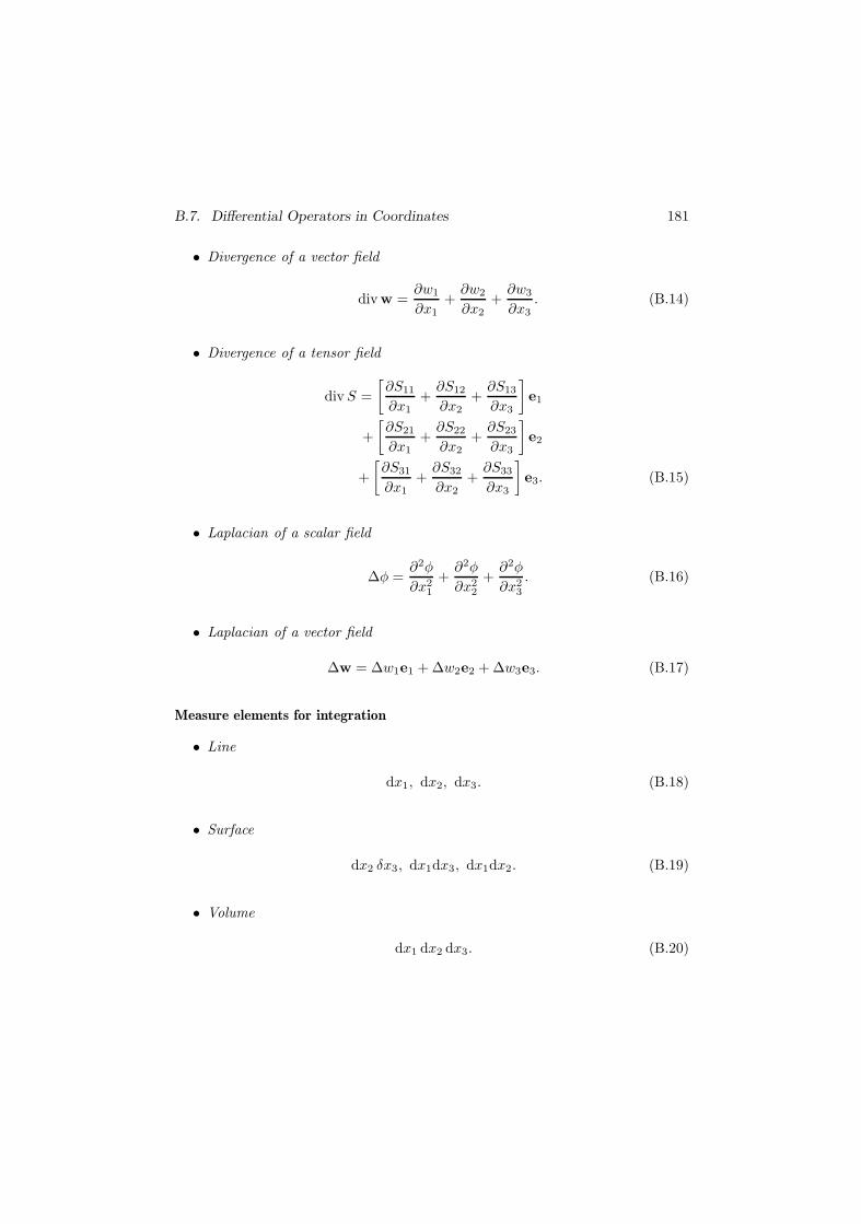
B.7. Differential Operators in Coordinates 181
• Divergence of a vector field
div w =∂w1
∂x1+
∂w2
∂x2+
∂w3
∂x3. (B.14)
• Divergence of a tensor field
div S =[∂S11
∂x1+
∂S12
∂x2+
∂S13
∂x3
]e1
+[∂S21
∂x1+
∂S22
∂x2+
∂S23
∂x3
]e2
+[∂S31
∂x1+
∂S32
∂x2+
∂S33
∂x3
]e3. (B.15)
• Laplacian of a scalar field
∆φ =∂2φ
∂x21
+∂2φ
∂x22
+∂2φ
∂x23
. (B.16)
• Laplacian of a vector field
∆w = ∆w1e1 + ∆w2e2 + ∆w3e3. (B.17)
Measure elements for integration
• Line
dx1, dx2, dx3. (B.18)
• Surface
dx2 δx3, dx1dx3, dx1dx2. (B.19)
• Volume
dx1 dx2 dx3. (B.20)
182 Appendix B. Vector and Tensor Analysis
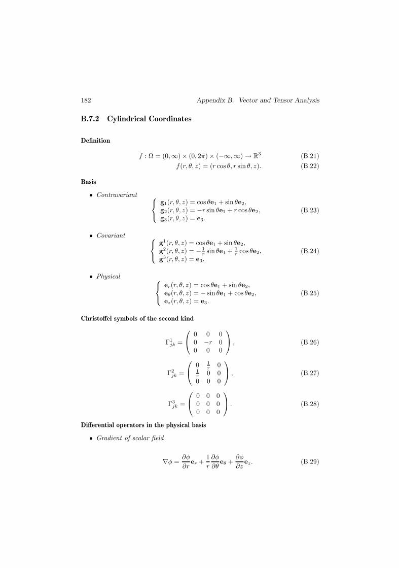
B.7.2 Cylindrical Coordinates
Definition
f : Ω = (0,∞) × (0, 2π) × (−∞,∞) → R3 (B.21)
f(r, θ, z) = (r cos θ, r sin θ, z). (B.22)
Basis
• Contravariant ⎧⎨⎩g1(r, θ, z) = cos θe1 + sin θe2,g2(r, θ, z) = −r sin θe1 + r cos θe2,g3(r, θ, z) = e3.
(B.23)
• Covariant ⎧⎨⎩g1(r, θ, z) = cos θe1 + sin θe2,g2(r, θ, z) = − 1
r sin θe1 + 1r cos θe2,
g3(r, θ, z) = e3.(B.24)
• Physical ⎧⎨⎩er(r, θ, z) = cos θe1 + sin θe2,eθ(r, θ, z) = − sin θe1 + cos θe2,ez(r, θ, z) = e3.
(B.25)
Christoffel symbols of the second kind
Γ1jk =
⎛⎝ 0 0 00 −r 00 0 0
⎞⎠ , (B.26)
Γ2jk =
⎛⎝ 0 1r 0
1r 0 00 0 0
⎞⎠ , (B.27)
Γ3jk =
⎛⎝ 0 0 00 0 00 0 0
⎞⎠ . (B.28)
Differential operators in the physical basis
• Gradient of scalar field
∇φ =∂φ
∂rer +
1r
∂φ
∂θeθ +
∂φ
∂zez. (B.29)
B.7. Differential Operators in Coordinates 183
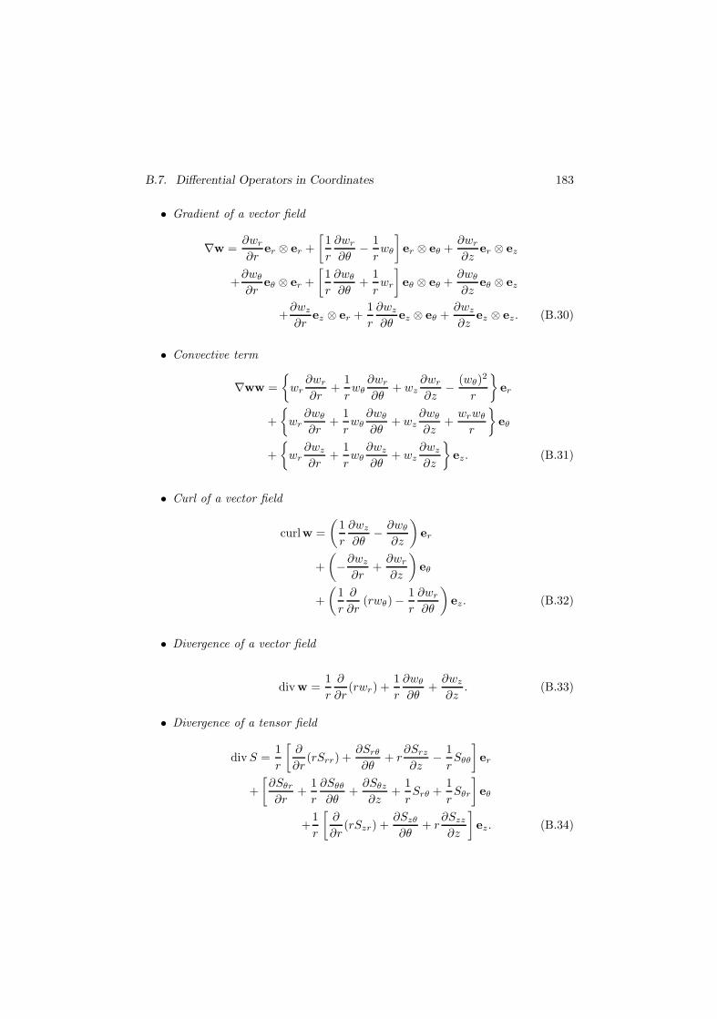
• Gradient of a vector field
∇w =∂wr
∂rer ⊗ er +
[1r
∂wr
∂θ− 1
rwθ
]er ⊗ eθ +
∂wr
∂zer ⊗ ez
+∂wθ
∂reθ ⊗ er +
[1r
∂wθ
∂θ+
1rwr
]eθ ⊗ eθ +
∂wθ
∂zeθ ⊗ ez
+∂wz
∂rez ⊗ er +
1r
∂wz
∂θez ⊗ eθ +
∂wz
∂zez ⊗ ez. (B.30)
• Convective term
∇ww =
wr∂wr
∂r+
1rwθ
∂wr
∂θ+ wz
∂wr
∂z− (wθ)2
r
er
+
wr∂wθ
∂r+
1rwθ
∂wθ
∂θ+ wz
∂wθ
∂z+
wrwθ
r
eθ
+
wr∂wz
∂r+
1rwθ
∂wz
∂θ+ wz
∂wz
∂z
ez. (B.31)
• Curl of a vector field
curlw =(
1r
∂wz
∂θ− ∂wθ
∂z
)er
+(−∂wz
∂r+
∂wr
∂z
)eθ
+(
1r
∂
∂r(rwθ) −
1r
∂wr
∂θ
)ez. (B.32)
• Divergence of a vector field
div w =1r
∂
∂r(rwr) +
1r
∂wθ
∂θ+
∂wz
∂z. (B.33)
• Divergence of a tensor field
div S =1r
[∂
∂r(rSrr) +
∂Srθ
∂θ+ r
∂Srz
∂z− 1
rSθθ
]er
+[∂Sθr
∂r+
1r
∂Sθθ
∂θ+
∂Sθz
∂z+
1rSrθ +
1rSθr
]eθ
+1r
[∂
∂r(rSzr) +
∂Szθ
∂θ+ r
∂Szz
∂z
]ez. (B.34)
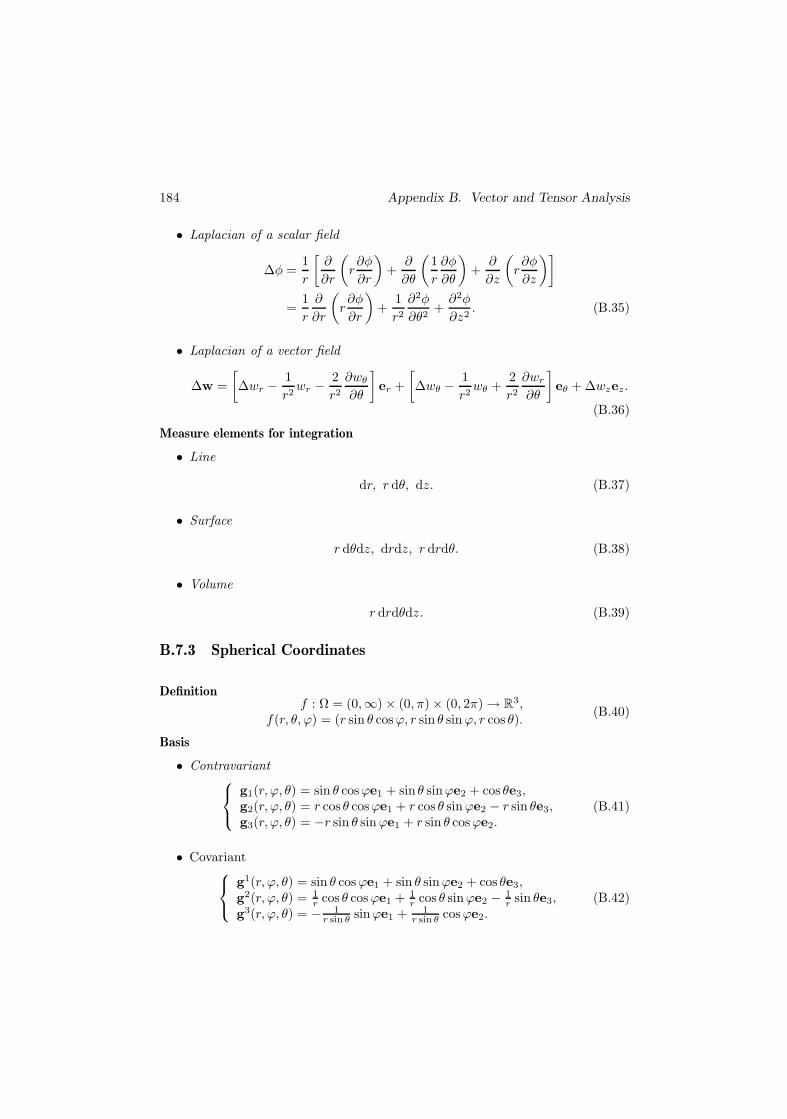
184 Appendix B. Vector and Tensor Analysis
• Laplacian of a scalar field
∆φ =1r
[∂
∂r
(r∂φ
∂r
)+
∂
∂θ
(1r
∂φ
∂θ
)+
∂
∂z
(r∂φ
∂z
)]=
1r
∂
∂r
(r∂φ
∂r
)+
1r2
∂2φ
∂θ2+
∂2φ
∂z2. (B.35)
• Laplacian of a vector field
∆w =[∆wr −
1r2
wr −2r2
∂wθ
∂θ
]er +
[∆wθ −
1r2
wθ +2r2
∂wr
∂θ
]eθ + ∆wzez.
(B.36)
Measure elements for integration
• Line
dr, r dθ, dz. (B.37)
• Surface
r dθdz, drdz, r drdθ. (B.38)
• Volume
r drdθdz. (B.39)
B.7.3 Spherical Coordinates
Definitionf : Ω = (0,∞) × (0, π) × (0, 2π) → R
3,f(r, θ, ϕ) = (r sin θ cosϕ, r sin θ sin ϕ, r cos θ). (B.40)
Basis
• Contravariant⎧⎨⎩g1(r, ϕ, θ) = sin θ cosϕe1 + sin θ sinϕe2 + cos θe3,g2(r, ϕ, θ) = r cos θ cosϕe1 + r cos θ sin ϕe2 − r sin θe3,g3(r, ϕ, θ) = −r sin θ sin ϕe1 + r sin θ cosϕe2.
(B.41)
• Covariant⎧⎨⎩g1(r, ϕ, θ) = sin θ cosϕe1 + sin θ sin ϕe2 + cos θe3,g2(r, ϕ, θ) = 1
r cos θ cosϕe1 + 1r cos θ sin ϕe2 − 1
r sin θe3,g3(r, ϕ, θ) = − 1
r sin θ sinϕe1 + 1r sin θ cosϕe2.
(B.42)
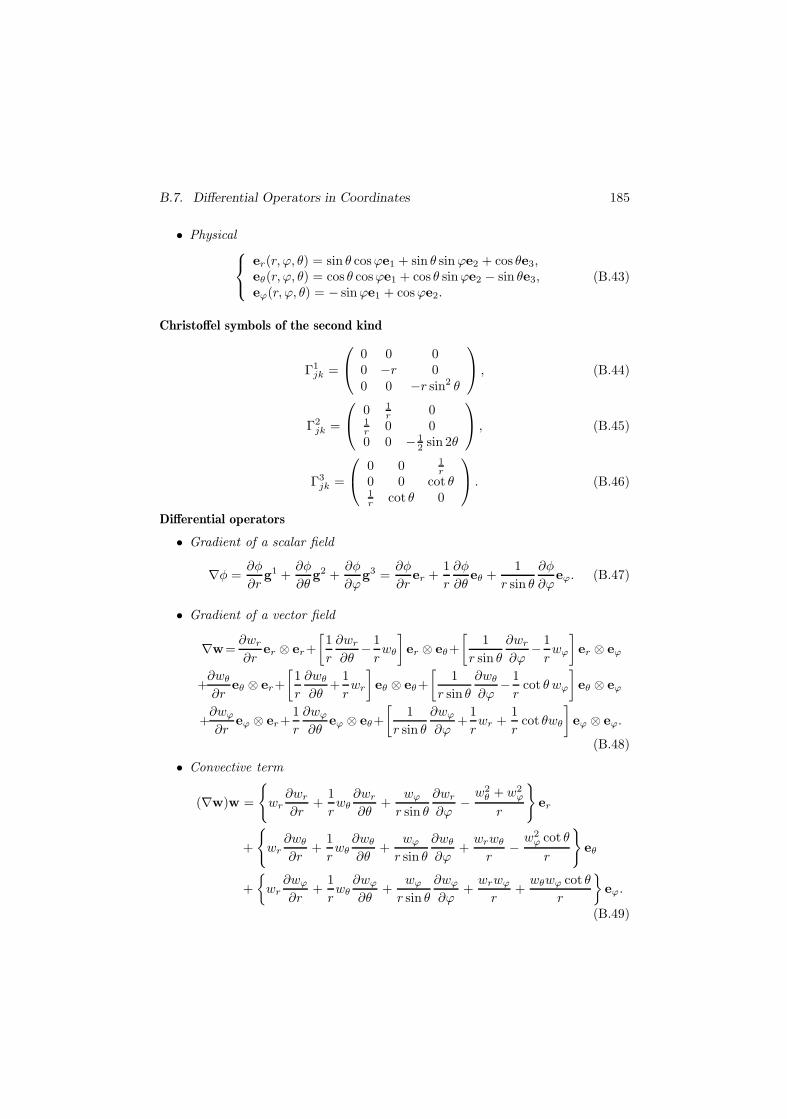
B.7. Differential Operators in Coordinates 185
• Physical⎧⎨⎩er(r, ϕ, θ) = sin θ cosϕe1 + sin θ sin ϕe2 + cos θe3,eθ(r, ϕ, θ) = cos θ cosϕe1 + cos θ sinϕe2 − sin θe3,eϕ(r, ϕ, θ) = − sinϕe1 + cosϕe2.
(B.43)
Christoffel symbols of the second kind
Γ1jk =
⎛⎝ 0 0 00 −r 00 0 −r sin2 θ
⎞⎠ , (B.44)
Γ2jk =
⎛⎝ 0 1r 0
1r 0 00 0 − 1
2 sin 2θ
⎞⎠ , (B.45)
Γ3jk =
⎛⎝ 0 0 1r
0 0 cot θ1r cot θ 0
⎞⎠ . (B.46)
Differential operators
• Gradient of a scalar field
∇φ =∂φ
∂rg1 +
∂φ
∂θg2 +
∂φ
∂ϕg3 =
∂φ
∂rer +
1r
∂φ
∂θeθ +
1r sin θ
∂φ
∂ϕeϕ. (B.47)
• Gradient of a vector field
∇w=∂wr
∂rer ⊗ er+
[1r
∂wr
∂θ− 1
rwθ
]er ⊗ eθ+
[1
r sin θ
∂wr
∂ϕ− 1
rwϕ
]er ⊗ eϕ
+∂wθ
∂reθ ⊗ er+
[1r
∂wθ
∂θ+
1rwr
]eθ ⊗ eθ+
[1
r sin θ
∂wθ
∂ϕ− 1
rcot θ wϕ
]eθ ⊗ eϕ
+∂wϕ
∂reϕ ⊗ er+
1r
∂wϕ
∂θeϕ ⊗ eθ+
[1
r sin θ
∂wϕ
∂ϕ+
1rwr +
1r
cot θwθ
]eϕ ⊗ eϕ.
(B.48)
• Convective term
(∇w)w =
wr
∂wr
∂r+
1rwθ
∂wr
∂θ+
wϕ
r sin θ
∂wr
∂ϕ−
w2θ + w2
ϕ
r
er
+
wr
∂wθ
∂r+
1rwθ
∂wθ
∂θ+
wϕ
r sin θ
∂wθ
∂ϕ+
wrwθ
r−
w2ϕ cot θ
r
eθ
+
wr∂wϕ
∂r+
1rwθ
∂wϕ
∂θ+
wϕ
r sin θ
∂wϕ
∂ϕ+
wrwϕ
r+
wθwϕ cot θ
r
eϕ.
(B.49)
186 Appendix B. Vector and Tensor Analysis
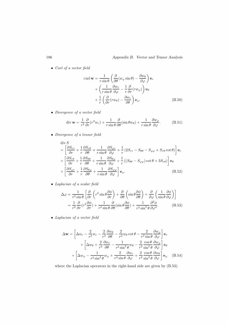
• Curl of a vector field
curlw =1
r sin θ
(∂
∂θ(wϕ sin θ) − ∂wθ
∂ϕ
)er
+(
1r sin θ
∂wr
∂ϕ− 1
r
∂
∂r(rwϕ)
)eθ
+1r
(∂
∂r(rwθ) −
∂wr
∂θ
)eϕ. (B.50)
• Divergence of a vector field
div w =1r2
∂
∂r(r2wr) +
1r sin θ
∂
∂θ(sin θwθ) +
1r sin θ
∂wϕ
∂ϕ. (B.51)
• Divergence of a tensor field
div S
=[∂Srr
∂r+
1r
∂Srθ
∂θ+
1r sin θ
∂Sϕr
∂ϕ+
1r
(2Srr − Sθθ − Sϕϕ + Srθ cot θ)]er
+[∂Srθ
∂r+
1r
∂Sθθ
∂θ+
1r sin θ
∂Sθϕ
∂ϕ+
1r
((Sθθ − Sϕϕ) cot θ + 3Srθ)]eθ
+[∂Sϕr
∂r+
1r
∂Sθϕ
∂θ+
1r sin θ
∂Sϕϕ
∂ϕ
]eϕ. (B.52)
• Laplacian of a scalar field
∆ϕ =1
r2 sin θ
[∂
∂r
(r2 sin θ
∂φ
∂r
)+
∂
∂θ
(sin θ
∂φ
∂θ
)+
∂
∂ϕ
(1
sin θ
∂φ
∂ϕ
)]=
1r2
∂
∂r(r2 ∂φ
∂r) +
1r2 sin θ
∂
∂θ(sin θ
∂φ
∂θ) +
1r2 sin2 θ
∂2φ
∂ϕ2. (B.53)
• Laplacian of a vector field
∆w =[∆wr −
2r2
wr −2r2
∂wθ
∂θ− 2
r2wθ cot θ − 2
r2 sin θ
∂wϕ
∂ϕ
]er
+[∆wθ +
2r2
∂wr
∂θ− 1
r2 sin2 θwθ − 2
r2
cos θ
sin2 θ
∂wϕ
∂ϕ
]eθ
+[∆wϕ − 1
r2 sin2 θwϕ +
2r2 sin θ
∂wr
∂ϕ+
2r2
cos θ
sin2 θ
∂wθ
∂ϕ
]eϕ (B.54)
where the Laplacian operators in the right-hand side are given by (B.53).
B.7. Differential Operators in Coordinates 187
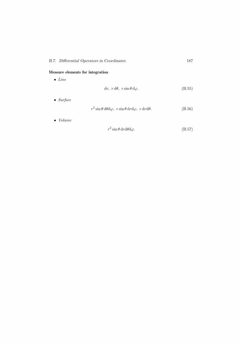
Measure elements for integration
• Line
dr, r dθ, r sin θ dϕ. (B.55)
• Surface
r2 sin θ dθdϕ, r sin θ drdϕ, r drdθ. (B.56)
• Volume
r2 sin θ drdθdϕ. (B.57)
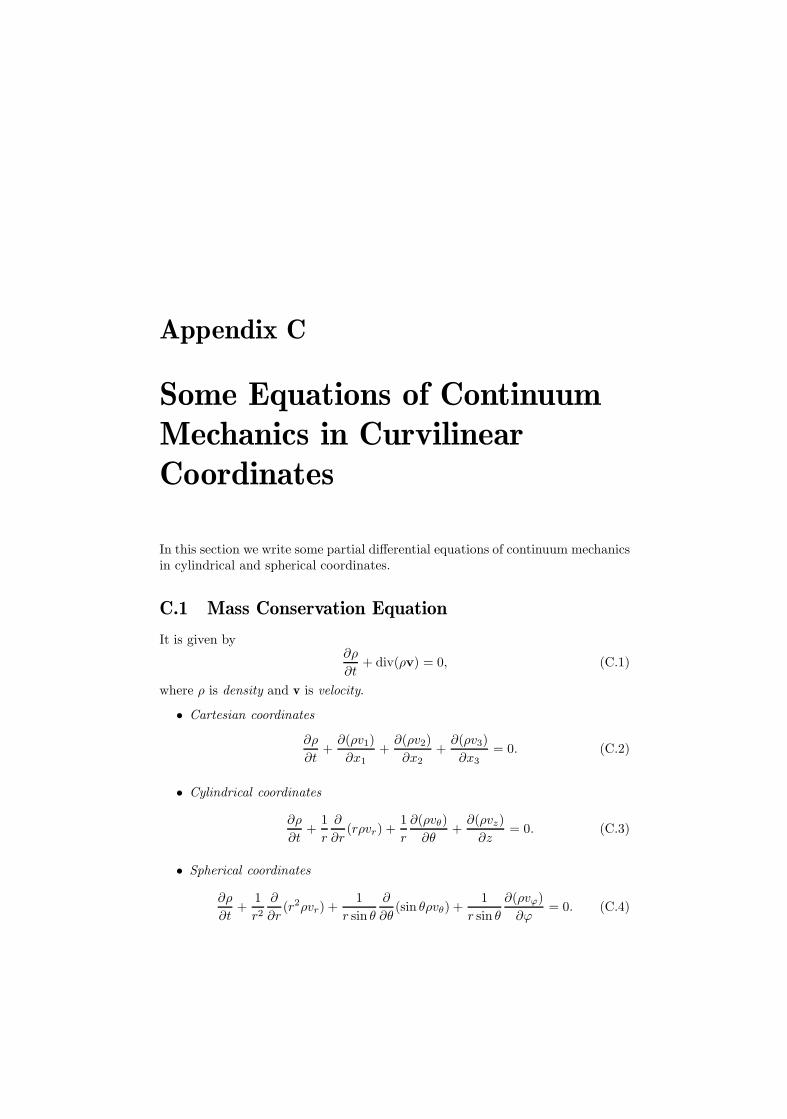
Appendix C
Some Equations of ContinuumMechanics in CurvilinearCoordinates
In this section we write some partial differential equations of continuum mechanicsin cylindrical and spherical coordinates.
C.1 Mass Conservation Equation
It is given by∂ρ
∂t+ div(ρv) = 0, (C.1)
where ρ is density and v is velocity.
• Cartesian coordinates
∂ρ
∂t+
∂(ρv1)∂x1
+∂(ρv2)∂x2
+∂(ρv3)∂x3
= 0. (C.2)
• Cylindrical coordinates
∂ρ
∂t+
1r
∂
∂r(rρvr) +
1r
∂(ρvθ)∂θ
+∂(ρvz)
∂z= 0. (C.3)
• Spherical coordinates
∂ρ
∂t+
1r2
∂
∂r(r2ρvr) +
1r sin θ
∂
∂θ(sin θρvθ) +
1r sin θ
∂(ρvϕ)∂ϕ
= 0. (C.4)
190 Appendix C. Some Equations in Curvilinear Coordinates
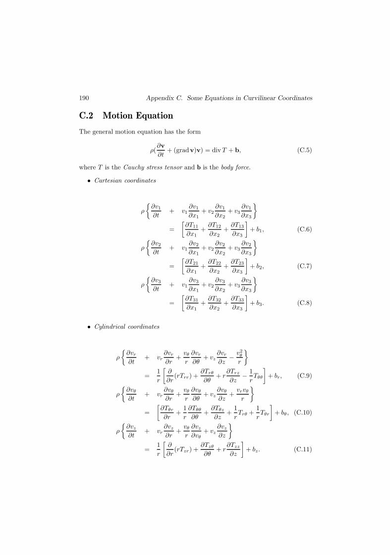
C.2 Motion Equation
The general motion equation has the form
ρ(∂v∂t
+ (gradv)v) = div T + b, (C.5)
where T is the Cauchy stress tensor and b is the body force.
• Cartesian coordinates
ρ
∂v1
∂t+ v1
∂v1
∂x1+ v2
∂v1
∂x2+ v3
∂v1
∂x3
=
[∂T11
∂x1+
∂T12
∂x2+
∂T13
∂x3
]+ b1, (C.6)
ρ
∂v2
∂t+ v1
∂v2
∂x1+ v2
∂v2
∂x2+ v3
∂v2
∂x3
=
[∂T21
∂x1+
∂T22
∂x2+
∂T23
∂x3
]+ b2, (C.7)
ρ
∂v3
∂t+ v1
∂v3
∂x1+ v2
∂v3
∂x2+ v3
∂v3
∂x3
=
[∂T31
∂x1+
∂T32
∂x2+
∂T33
∂x3
]+ b3. (C.8)
• Cylindrical coordinates
ρ
∂vr
∂t+ vr
∂vr
∂r+
vθ
r
∂vr
∂θ+ vz
∂vr
∂z− v2
θ
r
=
1r
[∂
∂r(rTrr) +
∂Trθ
∂θ+ r
∂Trz
∂z− 1
rTθθ
]+ br, (C.9)
ρ
∂vθ
∂t+ vr
∂vθ
∂r+
vθ
r
∂vθ
∂θ+ vz
∂vθ
∂z+
vrvθ
r
=
[∂Tθr
∂r+
1r
∂Tθθ
∂θ+
∂Tθz
∂z+
1rTrθ +
1rTθr
]+ bθ, (C.10)
ρ
∂vz
∂t+ vr
∂vz
∂r+
vθ
r
∂vz
∂vθ+ vz
∂vz
∂z
=
1r
[∂
∂r(rTzr) +
∂Tzθ
∂θ+ r
∂Tzz
∂z
]+ bz. (C.11)
C.3. Constitutive Law for Newtonian Viscous Fluids in Cooordinates 191
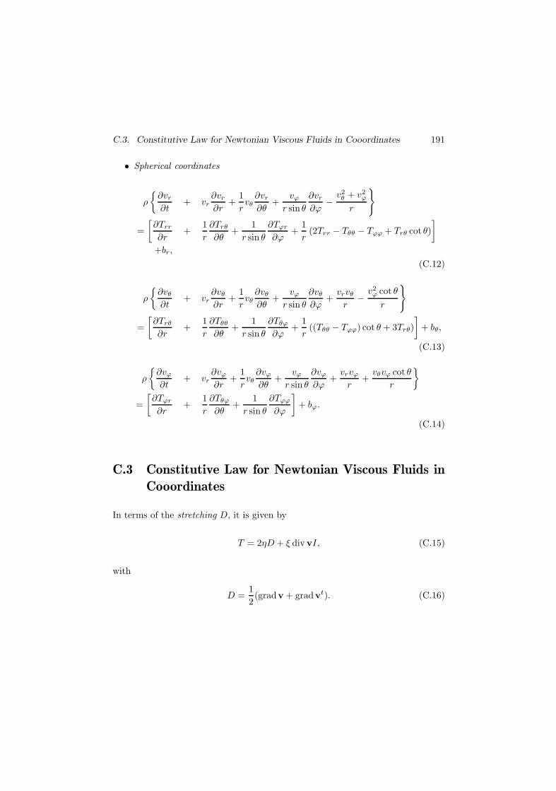
• Spherical coordinates
ρ
∂vr
∂t+ vr
∂vr
∂r+
1rvθ
∂vr
∂θ+
vϕ
r sin θ
∂vr
∂ϕ−
v2θ + v2
ϕ
r
=[∂Trr
∂r+
1r
∂Trθ
∂θ+
1r sin θ
∂Tϕr
∂ϕ+
1r
(2Trr − Tθθ − Tϕϕ + Trθ cot θ)]
+br,
(C.12)
ρ
∂vθ
∂t+ vr
∂vθ
∂r+
1rvθ
∂vθ
∂θ+
vϕ
r sin θ
∂vθ
∂ϕ+
vrvθ
r−
v2ϕ cot θ
r
=[∂Trθ
∂r+
1r
∂Tθθ
∂θ+
1r sin θ
∂Tθϕ
∂ϕ+
1r
((Tθθ − Tϕϕ) cot θ + 3Trθ)]
+ bθ,
(C.13)
ρ
∂vϕ
∂t+ vr
∂vϕ
∂r+
1rvθ
∂vϕ
∂θ+
vϕ
r sin θ
∂vϕ
∂ϕ+
vrvϕ
r+
vθvϕ cot θ
r
=[∂Tϕr
∂r+
1r
∂Tθϕ
∂θ+
1r sin θ
∂Tϕϕ
∂ϕ
]+ bϕ.
(C.14)
C.3 Constitutive Law for Newtonian Viscous Fluids inCooordinates
In terms of the stretching D, it is given by
T = 2ηD + ξ div vI, (C.15)
with
D =12(gradv + gradvt). (C.16)
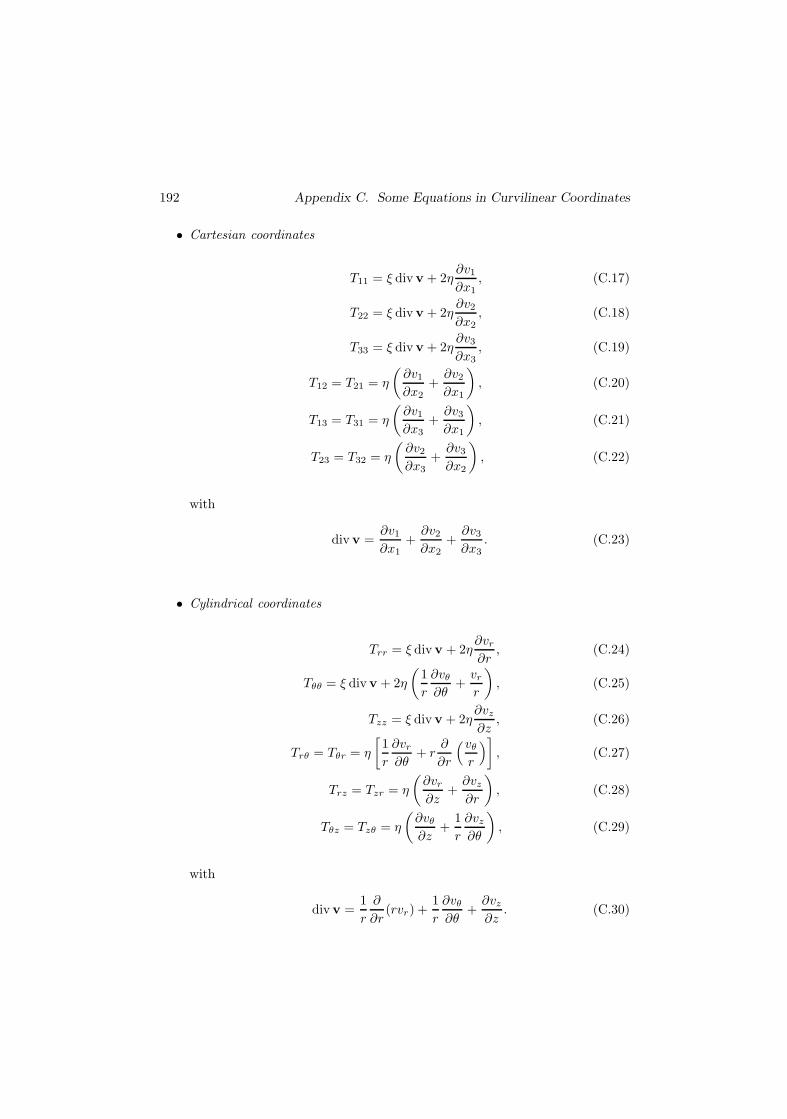
192 Appendix C. Some Equations in Curvilinear Coordinates
• Cartesian coordinates
T11 = ξ div v + 2η∂v1
∂x1, (C.17)
T22 = ξ div v + 2η∂v2
∂x2, (C.18)
T33 = ξ div v + 2η∂v3
∂x3, (C.19)
T12 = T21 = η
(∂v1
∂x2+
∂v2
∂x1
), (C.20)
T13 = T31 = η
(∂v1
∂x3+
∂v3
∂x1
), (C.21)
T23 = T32 = η
(∂v2
∂x3+
∂v3
∂x2
), (C.22)
with
div v =∂v1
∂x1+
∂v2
∂x2+
∂v3
∂x3. (C.23)
• Cylindrical coordinates
Trr = ξ div v + 2η∂vr
∂r, (C.24)
Tθθ = ξ div v + 2η
(1r
∂vθ
∂θ+
vr
r
), (C.25)
Tzz = ξ div v + 2η∂vz
∂z, (C.26)
Trθ = Tθr = η
[1r
∂vr
∂θ+ r
∂
∂r
(vθ
r
)], (C.27)
Trz = Tzr = η
(∂vr
∂z+
∂vz
∂r
), (C.28)
Tθz = Tzθ = η
(∂vθ
∂z+
1r
∂vz
∂θ
), (C.29)
with
div v =1r
∂
∂r(rvr) +
1r
∂vθ
∂θ+
∂vz
∂z. (C.30)
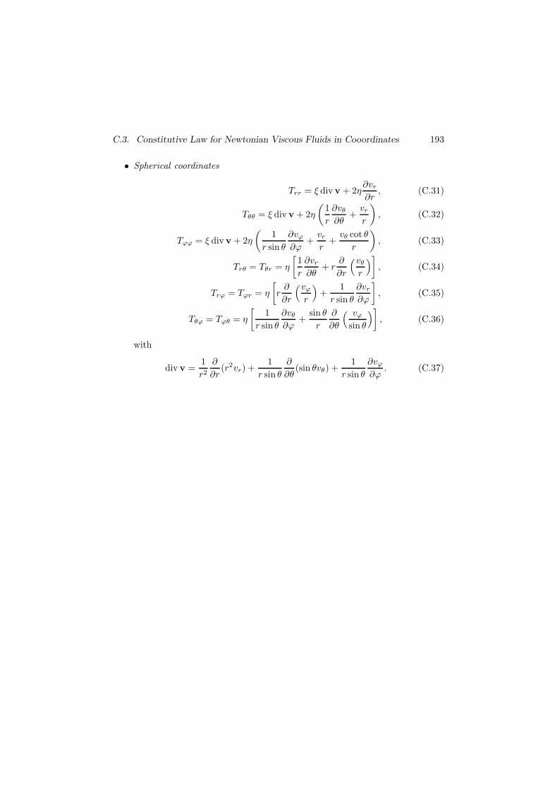
C.3. Constitutive Law for Newtonian Viscous Fluids in Cooordinates 193
• Spherical coordinates
Trr = ξ div v + 2η∂vr
∂r, (C.31)
Tθθ = ξ div v + 2η
(1r
∂vθ
∂θ+
vr
r
), (C.32)
Tϕϕ = ξ div v + 2η
(1
r sin θ
∂vϕ
∂ϕ+
vr
r+
vθ cot θ
r
), (C.33)
Trθ = Tθr = η
[1r
∂vr
∂θ+ r
∂
∂r
(vθ
r
)], (C.34)
Trϕ = Tϕr = η
[r
∂
∂r
(vϕ
r
)+
1r sin θ
∂vr
∂ϕ
], (C.35)
Tθϕ = Tϕθ = η
[1
r sin θ
∂vθ
∂ϕ+
sin θ
r
∂
∂θ
( vϕ
sin θ
)], (C.36)
with
div v =1r2
∂
∂r(r2vr) +
1r sin θ
∂
∂θ(sin θvθ) +
1r sin θ
∂vϕ
∂ϕ. (C.37)
Appendix D
Arbitrary Lagrangian-Eulerian(ALE) Formulations of theConservation Equations
In some fluid-structure interaction problems, the domain where the motion of thefluid is taking place changes with time because the structure interacting withthe fluid also moves. This is the case, for instance, of aeroelasticity problems.Moreover, there are free boundary flows for which the sets Bt, i.e., the positionsoccupied by the body, change with time and are a priori unknown. In these twosituations, numerical methods based on so-called Arbitrary Lagrangian-Eulerian(ALE) formulations can be very useful.
The main goal of this chapter is to write several ALE formulations of theconservation laws.
D.1 ALE Configuration
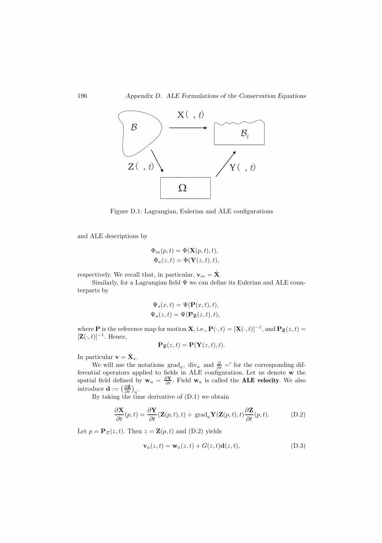
The situation is summarized in Figure D.1. Recall that B is the reference or La-grangian configuration, Bt is the Eulerian configuration and Ω denotes the ALEconfiguration. Y(·, t) is a motion transforming Ω into Bt at each time t and
Z(·, t) = [Y(·, t)]−1 X(·, t).
Hence,Y(Z(p, t), t) = X(p, t). (D.1)
Fields can be written in terms of Eulerian (spatial), Lagrangian (material) or ALEconfiguration. More precisely, if Φ is an Eulerian field, we can define its Lagrangian
196 Appendix D. ALE Formulations of the Conservation Equations
Z( , )t Y( , )t
X( , )t
BBt
Figure D.1: Lagrangian, Eulerian and ALE configurations
and ALE descriptions by
Φm(p, t) = Φ(X(p, t), t),Φa(z, t) = Φ(Y(z, t), t),
respectively. We recall that, in particular, vm = X.Similarly, for a Lagrangian field Ψ we can define its Eulerian and ALE coun-
terparts by
Ψs(x, t) = Ψ(P(x, t), t),Ψa(z, t) = Ψ(PZ(z, t), t),
where P is the reference map for motion X, i.e., P(·, t) = [X(·, t)]−1, and PZ(z, t) =[Z(·, t)]−1. Hence,
PZ(z, t) = P(Y(z, t), t).
In particular v = Xs.We will use the notations grada, diva and ∂
∂t =′ for the corresponding dif-ferential operators applied to fields in ALE configuration. Let us denote w thespatial field defined by wa = ∂Y
∂t . Field wa is called the ALE velocity. We alsointroduce d :=
(∂Z∂t
)a.
By taking the time derivative of (D.1) we obtain
∂X∂t
(p, t) =∂Y∂t
(Z(p, t), t) + gradaY(Z(p, t), t)∂Z∂t
(p, t). (D.2)
Let p = PZ(z, t). Then z = Z(p, t) and (D.2) yields
va(z, t) = wa(z, t) + G(z, t)d(z, t), (D.3)
D.2. Conservative ALE Form of Conservation Equations 197
where G denotes the tensor field gradaY.For a part P of B, let us denote by Pa
t the subset of Ω given by
Pat = Z(P , t).
Then, from the Reynolds Transport Theorem we get
Theorem 4.1.1. Let ϕ and Φ be an ALE scalar field and an ALE vector field,respectively. Then
d
dt
∫Pa
t
ϕdVz =∫Pa
t
ϕ′ dVz +∫Pa
t
diva(ϕd) dVz , (D.4)
d
dt
∫Pa
t
Φ dVz =∫Pa
t
Φ′ dVz +∫Pa
t
diva(Φ⊗ d) dVz . (D.5)
Corollary 4.1.2. We have
1. d
dt
∫Pa
t
ϕdVz =∫Pa
t
ϕ′ dVz +∫Pa
t
diva
[ϕG−1(va − wa)
]dVz, (D.6)
2. d
dt
∫Pa
t
Φ dVz =∫Pa
t
Φ′ dVz +∫Pa
t
diva
[Φ⊗ (va − wa)] G−t
dVz . (D.7)
Proof. It is an immediate consequence of (D.3). Indeed, we get d = G−1(va −wa)and then
diva(Φ ⊗ d) = diva
[Φ ⊗ G−1(va − wa)
]= diva
[Φ⊗ (va − wa)] G−t
. (D.8)
D.2 Conservative ALE Form of Conservation Equations
Now we are in a position to obtain the ALE formulations of the conservation equa-tions in conservative form. For this purpose we recall the conservation principlesin integral form and Eulerian coordinates, namely,
• Massd
dt
∫Pt
ρ dVx = 0. (D.9)
• Linear Momentum
d
dt
∫Pt
ρv dVx =∫
∂Pt
Tn dAx +∫Pt
b dVx. (D.10)
198 Appendix D. ALE Formulations of the Conservation Equations
• Energy
d
dt
∫Pt
ρE dVx =∫
∂Pt
Tn ·vdAx +∫Pt
b ·v dVx −∫
∂Pt
q ·n dAx +∫Pt
f dVx.
(D.11)
The corresponding ALE formulations are obtained by making, first, the change ofvariable x = Y(z, t) in the integrals. Let J(z, t) = detG(z, t) and Pt = Y(Pa
t , t).We have
• Massd
dt
∫Pa
t
ρaJ dVz = 0. (D.12)
By using (D.11) for ϕ = ρaJ we obtain∫Pa
t
(ρaJ)′ + diva
[ρaJG−1(va − wa)
]dVz = 0, (D.13)
and hence, from the Localization Theorem,
(ρaJ)′ + diva
[ρaJG−1(va − wa)
]= 0. (D.14)
• Linear momentum
d
dt
∫Pa
t
ρaJ dVz =∫
∂Pat
JTaG−tm dAz +∫Pa
t
Jba dVz . (D.15)
We transform this equality by using (D.7) for Φ = ρaJva and Gauss’ Theo-rem. We obtain∫
Pat
[(ρavaJ)′ + diva
ρaJ [va ⊗ (va − wa)]G−t
]dVz (D.16)
=∫Pa
t
diva
[JTaG
−t]dVz +
∫Pa
t
Jba dVz, (D.17)
and then, the Localization Theorem yields
(ρavaJ)′ + diva
J [ρava ⊗ (va − wa) − Ta]G−t
= Jba. (D.18)
• Energy
d
dt
∫Pa
t
ρaEaJ dVz =∫
∂Pat
JTava · G−tm dAz (D.19)
+∫Pa
t
Jba · va dVz −∫
∂Pat
Jqa · G−tm dAz +∫Pa
t
Jfa dVz . (D.20)
D.2. Conservative ALE Form of Conservation Equations 199
By using (D.11) for ϕ = ρaEaJ and Gauss’ Theorem, this equality becomes∫Pa
t
(ρaEaJ)′ + diva
[ρaEaJG−1(va − wa)
]dVz
=∫Pa
t
diva
(JG−1Tava
)dVz +
∫Pa
t
Jba · va dVz
−∫Pa
t
diva
(JG−1qa
)dVz +
∫Pa
t
Jfa dVz, (D.21)
and, from the Localization Theorem,
(ρaEaJ)′ + diva
JG−1 [ρaEa(va − wa) − Tava + qa]
= Jba · va + Jfa. (D.22)
Similar computations allow us to deduce the ALE formulation of the energy equa-tion in terms of the internal energy, e = E − 1
2 |v|2, namely,
(ρaeaJ)′ + diva
JG−1 [ρaea(va − wa) + qa]
= JTaG
−t · gradava + Jfa. (D.23)
We notice that ALE partial differential equations (D.14), (D.18), (D.22) and (D.23)hold in the fixed domain Ω.
D.2.1 Mixed Conservative ALE Form of the ConservationEquations
Now, we are going to deduce another conservative form to be called mixed formbecause it includes fields in both ALE and spatial configuration while only partialdifferential operators in the spatial configuration are involved. For this purpose wewill make extensive use of the following results:
Lemma 4.2.1. Let g be a vector spatial field and S a tensor spatial field. We have
diva
[JG−1ga
]= G−t · gradaga = J (divg)a , (D.24)
diva
[JSaG−t
]= J (div S)a . (D.25)
Proof. We use the following equalities:
diva(Rty) = R · graday + y · diva R, (D.26)
which holds for any smooth ALE tensor field R and vector field y, and
diva(JG−t) = 0 (Piola’s identity). (D.27)

200 Appendix D. ALE Formulations of the Conservation Equations
Firstly, from (D.26) and (D.27) we get
diva
[JG−1ga
]= diva
[JG−t
]· ga + JG−t · gradaga = JG−t · gradaga. (D.28)
Moreover, by the chain rule,
gradaga = ( gradg)a G (D.29)
and hence
( gradg)a = gradagaG−1. (D.30)
From this equality we deduce
(div g)a = tr ( gradg)a = tr(gradagaG−1
)= G−t · gradaga. (D.31)
Then, equality (D.24) follows by using this equality in (D.28).In order to prove (D.25) we recall that, from the definition of the divergence
operator of a tensor field, we have,
diva(JSaG−t) · e = diva
[JG−1St
ae]
= diva
[JG−t
]· St
ae
+JG−t · grada(Stae) = J
(div(Ste)
)a
= J (div S)a · e, (D.32)
for all vectors e, where we have used (D.26), (D.27), and (D.24) for y = Ste andR = JG−1.
From this Lemma, and (D.14), (D.18) and (D.22) we easily get
(ρaJ)′ + J (div [ρ(v − w)])a = 0, (D.33)(ρavaJ)′ + J (div [ρv ⊗ (v − w) − T ])a = Jba, (D.34)
(ρaEaJ)′ + J (div [ρE(v − w) − Tv + q])a = Jba · va + Jfa, (D.35)
respectively.
D.3 Mixed Nonconservative Form of ALE ConservationEquations
Finally, we want to obtain mixed nonconservative ALE formulations of the con-servation equations.
• Mass. Firstly we have,
(ρaJ)′ = ρ′aJ + ρaJ ′ = ρ′aJ + ρaJ (div w)a (D.36)
D.3. Mixed Nonconservative Form of ALE Conservation Equations 201
and
J (div [ρ(v − w)])a = J [( gradρ)a · (va − wa) + ρa (div(v − w))a]
= JGt( gradρ)a · G−1(va − wa) + Jρa (div(v − w))a
= J gradaρa · d + Jρa (div(v − w))a . (D.37)
Replacing these expressions in (D.33) we get
J (ρ′a + gradaρa · d) + Jρa (div v)a = 0 (D.38)
and finallyρa + ρa (div v)a = 0, (D.39)
where ρa denotes the material time derivative of ALE field ρa with respectto motion Z.
• Momentum. Firstly, we have
(ρaJva)′ = ρaJv′a + (ρaJ)′va (D.40)
and
J (div [ρv ⊗ (v − w)])a = Jva (div [ρ(v − w)])a
+Jρa ( gradv)a (va − wa) . (D.41)
We add these equalities and then subtract the mass conservation equation(D.33) multiplied by va. We get
(ρaJva)′ + J (div [ρv ⊗ (v − w)])a = Jρav′a + Jρa ( gradv)a (va − wa)
= Jρav′a + Jρa ( gradv)a GG−1 (va − wa) = Jρav′
a + Jρa gradavad
= Jρava.(D.42)
By replacing this equality in (D.34) we finally obtain
ρava − (div T )a = ba. (D.43)
• Energy. Firstly we have
(ρaJEa)′ = ρaJE′a + (ρaJ)′Ea (D.44)
and
J (div [ρE(v − w)])a = JEa (div [ρ(v − w)])a
+ Jρa ( gradE)a · (va − wa) . (D.45)
202 Appendix D. ALE Formulations of the Conservation Equations
We add these equalities and then subtract the mass conservation equation(D.33) multiplied by Ea. We get
(ρaJEa)′ + J (div [ρE(v − w)])a = JρaE′a + Jρa ( gradE)a · (va − wa)
= JρaE′a + Jρa ( gradE)a · GG−1 (va − wa) = JρaE′
a + Jρa gradaEa · d= JρaEa.
(D.46)
By replacing this equality in (D.35) we finally obtain
ρaEa − (div [Tv])a + (div q)a = ba · va + fa. (D.47)
Bibliography
[1] A. Bermudez, Obtaining the linear equations for the small perturbations of aflow. Mat. Notae XLI (2001/02), 123–138.
[2] P. G. Ciarlet, Mathematical Elasticity. North Holland, 1988.
[3] B. D. Coleman, W. Noll, Thermodynamics of viscosity, heat conduction andelasticity. Arch. for Rational Mech. and Anal., 13 (1963), 167–178. Also in TheFoundations of Mechanics and Thermodynamics. Springer. Berlin, 1974.
[4] Z. H. Guo, The representation theorem for isotropic, linear asymmetric stress-strain relations. J. Elasticity 13 (1983), 121–124.
[5] M. E. Gurtin, An Introduction to Continuum Mechanics. Academic Press, NewYork, 1981.
[6] K. K. Kuo, Principles of Combustion. John Wiley and Sons, Hoboken, N.J.,2005.
[7] B. Mohammadi, O. Pironneau, Analysis of the K-Epsilon Turbulence Model.John Wiley and Sons, 1994.
[8] W. Noll, Representations of certain isotropic tensor functions, Arch. Math. 21(1970), 87–90.
[9] W. R. Smith, R. W. Missen, Chemical Reaction Equilibrium Analysis: Theoryand Algorithms. John Wiley and Sons, 1982.
Index
β-function, 156
absolute temperature, 11acceleration, 3, 65accumulated thermal expansion, 59acoustic intensity, 91activation energy, 120activation temperature, 120affine space, 170ALE configuration
energy equation, 198linear momentum equation, 198mass equation, 198velocity, 196
Arbitrary Lagrangian-Eulerian (ALE)configuration, 195
Arrhenius law, 119associativity, 161atoms, 122axial vector, 168
balance of linear and angular momen-tum, 5
basis, 162bilinear, 163body, 1body force, 5, 137body heat, 8Boussinesq hypothesis, 106Boussinesq model, 79bulk viscosity, 64
calorically perfect, 95cartesian coordinate frame, 171
cartesian coordinates, 179constitutive law for Newtonian
viscous fluids, 192mass conservation equation, 189motion equation, 190
Cauchy’s hypothesis, 7Cauchy’s theorem, 8Cauchy-Green strain tensors, 2change of specific free energy, 128,
129, 131characteristic temperature of vibra-
tion, 95chemical affinity, 128, 134chemical equilibrium, 125chemical potential, 115Clausius-Duhem inequality, 11closure models, 106coefficient
of isothermal compressibility, 68of linear thermal expansion at
constant stress, 55of volumetric thermal expansion
at constant pressure, 67Coleman-Noll material, 18commutative group, 161commutativity, 161compatible, 132compressible Euler equations, 98compressible Navier-Stokes
equations, 98concentration
of species Ei, 111of the mixture, 112
conductive heat flux, 137coordinates, 162, 165, 169
206 Index
Crocco’s theorem, 66cross product, 167curl, 174curve, 175
closed, 175length, 175
curvilinear integral, 176cylindrical coordinates, 182
constitutive law for Newtonianviscous fluids, 192
mass conservation equation, 189motion equation, 190
Dalton’s law, 111deformation, 1density, 150
in the motion, 4of the mixture, 110reference, 4
deviatoric, 168differentiable, 173differential, 173diffusion velocity, 110, 135displacement, 2dissipation inequality, 19dissipation rate, 24dissipative acoustics, 81distance, 171distribution function, 154divergence, 174divergence theorem, 177double delta function, 156dynamic viscosity, 64, 103
eddy dynamic viscosity, 106, 107elastic fluid, 96elasticity tensor, 50element mass fractions, 150endomorphisms, 1energy, 126energy equation
conservative, 137linearized for thermoelasticity, 54non-conservative, 138
enthalpy, 64, 138, 142, 150of formation, 139of the mixture, 110standard, 124
entropy, 11of the mixture, 110
equilibrium constant, 129–131based on concentrations, 129based on partial pressures, 128
Euclidean affine space, 171Euclidean vector space, 163Eulerian field, 3Eulerian fluctuation, 90Eulerian fluctuation of pressure, 79expectation, 154, 155extended symmetry group, 37extent, 127, 130
Favre averaged, 155Fick’s law, 136, 137field, 173filter, 105first principle of thermodynamics, 8flow
adiabatic, 149fluid, 61
energy conservation law, 64energy equation, 70motion equation, 64
Fourier’s law, 42free energy, 12, 129frequency factor, 120full stoichiometric matrix, 133
generalized Hooke’s law, 52Gibbs free energy, 77, 114, 127, 130,
141, 142of formation, 97, 115of the mixture, 111, 114standard, 97
gradient, 173of the motion, 2
gravity force, 87Green’s formulas, 177
Index 207
Green-Lagrange strain tensor, 2Green-Saint Venant strain tensor, 2,
41
heat flux, 8heat rate, 8Helmholtz free energy, 12
of the mixture, 111hyperelastic material
with heat conduction and viscos-ity, 18
ideal fluid, 103ideal gases, 96incompressible Euler equations, 104incompressible Navier-Stokes
equations, 106incompressible Newtonian fluid, 101incremental methods, 57infinitesimal strain tensor, 2, 48inlets, 146inner product, 163, 166internal energy, 9
of formation, 123of the mixture, 110, 121standard, 123
invertible, 168isobaric process, 149isotropic, 164
k-atoms, 122, 140, 146k-moles, 112kernel, 132
Lagrangian coordinates, 13Lagrangian fields, 3Lame’s coefficients, 55Laplacian, 174least action principle, 125Lewis number, 138linearly independent, 162local equilibrium chemistry, 149local equilibrium problem, 141localization theorem, 179
Mach number, 142, 149mass, 126, 141, 142, 150
of the mixture, 120mass action law, 119mass conservation equation, 135
conservative, 136mass diffusion, 136mass diffusion coefficient, 138mass distribution, 4mass fraction, 110, 140, 146material body, 18
isotropic, 39material fields, 3material frame-indifference principle,
28material points, 1material time derivative, 6Mayer equation, 94mean value, 154mechanical energy, 91mechanical equilibrium, 77mixture fractions, 148, 150, 155molar fraction, 112molecular mass, 93
of the mixture, 112motion, 1motion equation
conservative, 5, 137linear approximation of the , 52non-conservative, 5, 137
natural convection, 78neutral element, 161non-dissipative acoustics, 85norm, 163
observer change, 27origin, 171orthogonal, 163, 168orthonormal, 163outlet, 146
passive scalars, 141Pekeris equation, 87
208 Index
perfect gas, 93coefficient of isothermal
compressibility, 94coefficient of thermal expansion,
94enthalpy, 93entropy, 94internal energy, 93sound speed, 94specific heat at constant
pressure, 93positive definite, 56, 163positivity, 126, 142, 143, 150potential theorem, 176power stress, 6pre-exponential exponent, 120pressure, 102
Lagrangian fluctuation, 86of the mixture, 111standard , 129
principal invariants, 169probability density functions (PDF),
153, 154probability space, 153
random variable, 153continuous, 154independent, 154
random vector, 154(jointly) continuous, 154distribution function, 154
rank, 132rate of total mass per unit volume,
146ratio of specific heats, 94real vector space, 161reference configuration, 1reference map, 3region
closed, 176open, 176regular, 176
response mappings, 18rotation, 168
Saint Venant-Kirchhoff material, 41Schmidt numbers, 156second principle of thermodynamics,
11second viscosity coefficient, 64simply connected, 176skew, 166skew part, 167Smagorinsky’s model, 106small deformations, 57sound speed, 72source of mass, 135sources, 146spatial fields, 3, 135species, 109
density, 109enthalpy, 109entropy, 109Gibbs free energy, 109Helmholtz free energy, 109internal energy, 109molecular mass, 109pressure, 109specific heat at constant
pressure, 110specific heat at constant volume,
109velocity, 109
specific heatat constant deformation, 34at constant pressure, 69
of the mixture, 124at constant volume, 67, 121
of the mixture, 111, 121spherical, 168spherical coordinates, 184
constitutive law for Newtonianviscous fluids, 193
mass conservation equation, 189motion equation, 191
stagnation enthalpy, 65, 98state law, 125, 126, 142, 150stirred tank, 119, 125, 140stoichiometric coefficients, 119
Index 209
stoichiometric method, 132Stokes’ theorem, 177streams, 148stress tensor
Boussinesq, 13Cauchy, 5First Piola-Kirchhoff, 13Piola-Lagrange, 13Reynolds, 106Second Piola-Kirchhoff, 13
surface force, 5surface heat, 8symmetric, 163, 166symmetric element, 161symmetric part, 167symmetry transformation, 37system of forces, 5system of generators, 162system of heat, 8, 120
tensor, 164positive definite, 168
tensor of thermal expansion at cons-tant stress, 51
tensor product, 165, 169the response of a material body is in-
dependent of the observer,27
theorem of power expended, 6thermal conductivity, 42, 138thermal enthalpy, 139thermodynamic pressure, 63thermodynamic process, 17
adiabatic, 25Eulerian, 25homentropic, 66isentropic, 24isochoric, 101steady, 66
thermomechanical equilibrium, 78total energy, 8, 98trace, 166trajectory, 2transpose, 166
turbulence models, 105turbulent dissipation rate, 107turbulent kinetic energy, 107turbulent Prandtl, 156
Vaisala-Bruntfrequency, 89tensor, 88
variance, 154, 155vectors, 162velocity, 3, 119
of the mixture, 110, 135
wall, 146wave equation, 87