vayenas modern aspects of electrochemistry no. 39
TRANSCRIPT

VAYENAS
modern aspects of electrochemistryno. 39
modernaspectsofelectrochemistryno. 39
Edited by C.G. VAYENAS

MODERN ASPECTS OF
ELECTROCHEMISTRY
No. 39
Modern Aspects of Electrochemistry
Modern Aspects of Electrochemistry, No. 38:
Solid State Electrochemistry encompassing modern equilibria
concepts, thermodymanics and kinetics of charge carriers in solids.
Electron transfer processes, with special sections devoted to
hydration of the proton and its heterogeneous transfer.
electrodeposition of metals.
the electrode materials for phosphoric acid electrolyte fuel-cells.
Applications of reflexology and electron microscopy to the materials
science aspect of metal electrodes.
Electroplating of metal matrix composites by codeposition of
suspended particles, a process that has improved physical and
electrochemical properties.
Modern Aspects of Electrochemistry, No. 37:
The kinetics of electrochemical hydrogen entry into metals and
alloys.
The electrochemistry, corrosion, and hydrogen embrittlement of
unalloyed titanium. This important chapter discusses pitting and
galvanostatic corrosion followed by a review of hydrogen
embrittlement emphasizing the formation of hydrides and their
effect on titanium’s mechanical properties.
Oxidative electrochemical processes of organics, introduces an
impressive model that distinguishes active (strong) and non-active
(weak) anodes.
Comprehensive discussions of fuel cells and Carnot engines; Nernst
law; analytical fuel cell modeling; reversible losses and Nernst loss;
driving forces. Includes new developments and applications of fuel
cells in trigeneration systems; coal/biomass fuel cell systems;
indirect carbon fuel cells; and direct carbon fuel cells.
Exploration of the catalytic effect of trace anions in outer-sphere
heterogeneous charge-transfer reactions.
Results of the experimental and theoretical investigations on
bridging electrolyte-water systems as to thermodynamic and
transport properties of aqueous and organic systems. Revised
version of chapter four in Number 35.
Electrosorption at electrodes and its relevance to electrocatalysis and
The behavior of Pt and other alloy electrocatalyst crystallites used as
and irreversible losses, multistage oxidation, and equipartition of

List of Contributors, MAE 39
Thomas Z. Fahidy
Department of Chemical Engineering, University of Waterloo,
Waterloo, Ontario, Canada N2L 3G1
Joo-Young Go
Department of Materials Science and Engineering, Korea
Advanced Institute of Science and Technology, 373-1,
Guseong-dong, Yuseong-gu, Daejeon, 305-701, Republic of Korea
Jane S. Murray
Department of Chemistry, University of New Orleans, New
Orleans, LA 70148
Peter Politzer
Department of Chemistry, University of New Orleans, New
Orleans, LA 70148
Su-Il Pyun
Department of Materials Science and Engineering, Korea
Advanced Institute of Science and Technology, 373-1, Guseong-dong, Yuseong-gu, Daejeon, 305-701, Republic of Korea
Ashok K. Vijh
Institut de recherche d’Hydro-Québec,
1800, Blvd. Lionel-Boulet, Varennes, Québec Canada J3X 1S1
Gregory X. Zhang
Teck Cominco, Product Technology Centre, Mississauga,
Ontario, Canada
MODERN ASPECTS OF
ELECTROCHEMISTRY
No. 39
Edited by
C. G. VAYENAS University of Patras
Patras, Greece
RALPH E. WHITE University of South Carolina
Columbia, South Carolina
and
MARIA E. GAMBOA-ADELCO Managing Editor
Superior, Colorado

C. G. Vayenas
Department of Chemical Engineering
University of Patras
Patras 265 00
Greece
ISBN-10: 0-387-23371-7 e-ISBN 0-387-31701-5
ISBN-13: 978-0387-23371-0
Printed on acid-free paper.
All rights reserved. This work may not be translated or copied in whole or in part
Media, Inc., 233 Spring Street, New York, NY 10013, USA), except for brief
excerpts in connection with reviews or scholarly analysis. Use in connection with
any form of information storage and retrieval, electronic adaptation, computer
software, or by similar or dissimilar methodology now known or hereafter
The use in this publication of trade names, trademarks, service marks, and similar
terms, even if they are not identified as such, is not to be taken as an expression of
opinion as to whether or not they are subject to proprietary rights.
Printed in the United States of America.
9 8 7 6 5 4 3 2 1
springer.com
Library of Congress Control Number: 2005939188
without the written permission of the publisher (Springer Science+Business
2006 Springer Science+Business Media,
developed is forbidden.
LLC
(TB/IBT)

Volume 39 is dedicated to the memory
of Professor Brian E. Conway, a leading
electrochemist, a splendid teacher, a
wonderful friend, a great man, whom
the entire electrochemical community
will always remember.
John O’M Bockris,
Ralph White,
Costas Vayenas, and
Maria Gamboa-Aldeco

Preface
This volume of Modern Aspects covers a wide spread of
topics presented in an authoritative, informative and instructive
manner by some internationally renowned specialists. Professors
Politzer and Dr. Murray provide a comprehensive description of
the various theoretical treatments of solute-solvent interactions,
including ion-solvent interactions. Both continuum and discrete
molecular models for the solvent molecules are discussed,
including Monte Carlo and molecular dynamics simulations. The
advantages and drawbacks of the resulting models and
computational approaches are discussed and the impressive
progress made in predicting the properties of molecular and ionic
solutions is surveyed.
The fundamental and applied electrochemistry of the
silicon/electrolyte interface is presented in an authoritative review
by Dr. Gregory Zhang, with emphasis in the preparation of porous
silicon, a material of significant technological interest, via anodic
dissolution of monocrystalline Si. The chapter shows eloquently
how fundamental electrokinetic principles can be utilized to
obtain the desired product morphology.
Markov chains theory provides a powerful tool for
modeling several important processes in electrochemistry and
electrochemical engineering, including electrode kinetics, anodic
deposit formation and deposit dissolution processes, electrolyzer
and electrochemical reactors performance and even reliability of
warning devices and repair of failed cells. The way this can be
done using the elegant Markov chains theory is described in lucid
manner by Professor Thomas Fahidy in a concise chapter which
gives to the reader only the absolutely necessary mathematics and
is rich in practical examples.
Electrochemical processes usually take place on rough
surfaces and interfaces and the use of fractal theory to describe
and characterize the geometric characteristics of surfaces and
interfaces can be of significant importance in electrochemical
process description and optimization. Drs. Joo-Young Go and

electrochemical methods used for the determination of surface
fractal dimensions and of the implications of fractal geometry in
the description of several important electrochemical systems,
including corroding surfaces as well as porous and composite
electrodes.
Electrochemistry plays an increasingly important role in
biology and medicine and the electrochemical treatment of tumors
(ECT) is receiving considerable attention as a viable alternative to
the more classical tumor treating approaches of surgery and
chemotherapy. Dr. A. Vijh, a specialist in this area, describes both
the phenomenology and the proposed physicochemical
mechanisms of ECT in a comprehensive chapter.
C.G. Vayenas
R.E. White
SSu-Il Pyun provide a comprehensive review of the physical and
Preface X

MEMORIES OF BRIAN EVANS CONWAY
EDITOR 1955-2005
By John O’M. Bockris (Editor 1953-2003)
I remember meeting Brian Conway on the road, Queens Gate,
which leads from Imperial College, London University, to the Tube
Station in South Kensington, London. It was a Saturday afternoon in
1946. I was one year into a lectureship (assistant professorship in
U.S. terms) at Imperial College, the technologically oriented part of
London University. Brian stopped me to say that he wanted to do his
graduate research with me. He was 20 and I, 23.
Brian Conway entered my research group at Imperial College
in its second year. There are some who have called the years
between 1946 and 1950 as the Golden Years of Electrochemistry
because the development of the subject as a part of physical
chemistry was pioneered in those years, primarily by the remarkable
set of people who were in the group at that time and who spread out
with their own students and ideas after they left me.
First among those in respect to the honors achieved was
Roger Parsons. He became an FRS and President of the Faraday
Division of the Chemical Society. Conway is No. 2 in this formal
ranking although he published more extensively and with more
original ideas than did Parsons. Then there was John Tomlinson who
became a professor at the University of Wellington in New Zealand
(and Vice Chancelor of the University). E.C. Potter too was in the
group at that time and became in the 1980's the President of the
Royal Society of New South Wales, apart from having an active
career in the Council of Science and Industry of the Australian
government. Harold Eagan was there too and he later achieved a
grand title: “The Government Chemist,” the man in the U.K.
government who is in charge of testing the purity of various
elements of the country’s supply.

XII
The only woman in the group, Hanna Rosenburg, should be
mentioned here because she had an extended influence on Brian
Conway, based partly on her remarkable ability to discuss widely.
Martin Fleischmann, too, is relevant. He got his Ph.D. in a
small group near to my group in which Conway worked. However,
he joined us in various activities, particularly the discussions. He
became well known internationally not only because of his
contributions to physical electrochemistry, but also because in 1989
he resuscitated an idea, - which had been introduced by the French
and Japanese in the 1960's, - that nuclear reactions could be carried
out in solutions in the cold.
Conway’s thesis (1949) was very original in content and
contained, e.g., 3 D representations of potential energy surfaces.
After Brian Conway got his Ph.D. with me, he went to work
with J.A.V. Butler at the Chester-Beatty Cancer Research Institute, a
short walk from Imperial College. Butler’s habit of pouring over
manuscripts, murmuring, and his sensitivity to noise whilst thinking,
was reflected by some of Conway’s habits. Butler was known to be
absent minded in a way which colored the great respect with which
he was regarded. Thus, according to Conway, in Butler’s year at
Uppsala he was observed by a British colleague to pass two lumps
of sugar to the cashier whilst thoughtfully adding the ore to his
coffee.
Contact with Conway continued from 1949 to 1953 in
London. We used to meet on Saturday afternoons in a Kensington
coffee shop and it was there that some of our electrochemical
problems were worked out.
After 1951, I decided to look towards the United States for
doc to take with us and wanted to get him married before the
transition. Unfortunately, Brian evaluated girls principally by their
intellectual abilities and the Viennese Ms. Rosenburg had given him
the model. He found it difficult to meet her equal and we had
eventually to point out to him that he couldn’t get a Visa to come to
America with a woman unless he were married to her. Shortly, after
this, he did invite me to Daguize, our Saturday café, to meet a
former Latvian pharmacist, Nina, and later I served to take Nina up
Memories of Brian Evans Conway
continuation of my career. We thought of Brian as a possible post
the aisle at the wedding of Nina and Brian (1954).

XIII
It had seemed to me that, if we were going to bring
Electrochemistry from its moribund state of the 1940's to modernity
in physical chemistry, a yearly monograph would help and I
therefore approached Butterworth’s in London with a proposition
and the first volume was published in 1954.1 I brought Brian into the
Aspects in Volume I as an assistant and also my co-author in a
chapter on solvation. It soon seemed unfair to continue to receive
Brian’s help in editing unless he was made an editor too and
therefore, from the second volume on, we were both named editors
of the series and kept it that way until, in 1987, we invited Ralph
White to join us as the Electrochemical Engineer, thus increasing the
breadth of the topics received.2
I moved to the University of Pennsylvania in Philadelphia in
1953 whilst Brian remained at Chester-Beatty, but I went back to
London for the summer of 1954 and persuaded Brian to come over
to Philadelphia at first as a post doctoral fellow.
Brian Conway’s move to the U.S.A. facilitated our joint
editorship in running the series. We had had many discussions in
London and this encouraged us to make the composition of each
volume an occasion for a Meeting, lasting two to three days in a
resort. This meant one to two day’s hard discussion deciding the
topics we wanted and then the authors who might write the articles,
together with a reserve author in case the first one refused. The third
day we spent as free time for our own discussions. Colorado Springs
was a place in which we had an interesting time and then there was
the Grand Hotel in White Sulfur Springs and several resorts in
Canada. But there is no doubt that Bermuda was more often the
locale of the Modern Aspects invitation meetings than any other.
After Ralph White threw his expertise onto choice of authors, we
continued to meet yearly, e.g., in Quebec City and in San Francisco,
though in recent years the meetings drifted back to their original
form.
1 Butterworth’s was purchased by Plenum Press in 1955 after the second volume for
Modern Aspects of Electrochemistry had been published.2 Our policy throughout, - as I believe it is with the present editors, - was to make in
Modern Aspects of Electrochemistry a truly broad presentation of the field although
we always avoided analytical topics for which there was already so much
presentation.
Memories of Brian Evans Conway

XIV
Coming now to Brian’s two years at the University of
Pennsylvania (1954-1955), we got out of this time three papers
which I think of as being foundation papers of what we now know as
physical electrochemistry. The first concerned the mechanism of the
high mobility of the proton in water. The second arose out of the
interpretation of plots of log io against the strength of the metal-
hydrogen bond and found two groups of metals, one involving
proton discharge onto planar sites and the other proton discharge
(rate determining) onto adsorbed H. The last of the three concerned
the early stages of metal deposition, a subject which raises many
fundamental questions in electrochemical theory (e.g., partial charge
transfer). The first two of these works were published in the Journal
of Chemical Physics and the last one in the Proceedings of the Royal
Society. To have papers accepted in these prestigious journals is
unusual and particularly for electrochemical topics so often mired in
lowly technological issues.
Conway transferred to the University of Ottawa in 1955 and
remained there for the rest of his career. He published near to 400
papers whilst in Ottawa and it’s interesting to mention a few of
them.
In Ottawa I would pick out the work with Currie in 1978 on
pressure dependence of electrode reactions. It gave a new
mechanism criterion.
Agar had suggested in 1947 that there might be a temperature
dependence of , the electrode kinetic parameter, and Conway took
this up in 1982 and showed experimentally that in certain reactions
this was the case.
The most well known work that Conway and his colleagues
completed in Ottawa was on the analysis of potential sweep curves. I
had been critical of the application of potential sweep theory to
reactions which involved intermediates on the electrode surface and,
working particularly early with Gilaedi and then with Halina
Kozlowska, and to some extent with Paul Stonehart, Conway
developed an analysis of the effect of intermediate radicals on the
shape and properties of potential sweep showing how interesting
electrode kinetic parameters could be thereby obtained.
This is the point to stress the part played by Halina
Angerstein-Kozlowska in Brian’s work. She played an important
role in administration of the co-workers, apart from the supervision
Memories of Brian Evans Conway

XV
of the work, particularly in Brian’s absences at meetings, many in
Europe. Her position was similar to that of the late Srinivasan in
respect to John Appleby electrochemical research group at Texas
A&M. It is more creative and directional than her formal position as
a senior researcher indicates.
I continued an active discussion relationship with Brian
Conway for more than fifty years. This was made possible not only
by the yearly meetings for Modern Aspects but by letters, most
which were in discussions of topics apart from electrochemistry. I
remember those on the inheritance of acquired characteristics with
Hanna Rosenburg in London in the fifties and the discussions of the
position and number of the galaxies and then later, consideration of
methods by aggressive groups could be restrained from war. In more
recent years we have been concerned with the speed of electrons in
telephone lines. Many people think that electrons there must travel
very quickly but in fact their movement during the passage of
messages is measured in a few cms per second.
Although the correspondence with me concerned topics
discussed in terms of the science of the day, Conway’s interests
were broad and he had interests in the Arts, stimulated by his wife in
this direction (his house was decorated with her paintings). In this
respect, Conway exemplifies the Scientist as a Great Man, a man of
Knowledge in all and any direction. One is reminded of Frumkin in
Moscow who kept abreast of modern literature from Anglo-
America, France and Germany and Hinshelwood at Oxford, a
physical chemist whose alternative interests were in Japanese
Poetry.
The long lasting scientific correspondence with Conway
started to ebb in the mid nineties and I assumed that this was due to
normal processes of aging but it turned out that it was the beginning
of the end, - he was frequently in the hospital.
One day in this Summer of 2005, Nina called to tell me that
the doctors declared the prostate cancer which he had suffered had
metastasized and that they could no longer control it. I placed myself
at Brian’s disposal in respect to anything that he wanted, - I worked
here through the well-known Barry Macdougall, an ex Conway
student. Through him I passed to Brian photographs from the
London days, and these contained, among others, the one he most
Memories of Brian Evans Conway

XVI
wanted, - that of the student he had known 55 years earlier, Hanna
Rosenburg.
Brian leaves behind him Nina (later a professional artist and
musician) who had contributed so much to his career by her help and
fortitude and a son, Adrian, who is a competent theorist in telephone
networks.
Brian chose to have his body cremated.
JOMB/ts
Memories of Brian Evans Conway

Contents
Chapter 1
QUANTITATIVE APPROACHES TO
SOLUTE-SOLVENT INTERACTIONS
Peter Politzer and Jane S. Murray
I. Introduction 1
II. General Interaction Properties Function (GIPF) ....... 3
1. Background ........................................................... 3
2. Applications .......................................................... 9
3. Summary ............................................................... 16
III. Procedures that Directly Address the Solute-Solvent
Interaction ................................................................. 17
1. Discrete Molecular Models of Solvent 17
2. Continuum Models of Solvent 26
3. Hybrid/Intermediate Models of Solvent 38
4. General Comments: Discrete Molecular and
Continuum Solvent Models .................................. 41
5. Ionic Solvation 41
IV. Linear Solvation Energy Relationships (LSER) ....... 51
1. Empirical ............................................................... 51
2. Theoretical ............................................................ 53
..............
......................................................
XVII
V. Discussion and Summary ......................................... 55
References................................................................. 56
Acknowledgement..................................................... 56
.................
..............................

Chapter 2
POROUS SILICON: MORPHOLOGY AND
FORMATION MECHANISMS
Gregory X. Zhang
2. Hydrogen evolution and effective dissolution
1. Potential distribution and rate limiting
3. Effect of geometric elements ............................... 103
5. Surface lattice structure........................................ 110
6. Reactions on the surfaces of silicon and silicon
7. Distribution of reactions and their rates
on pore bottoms ................................................ 115
8. Formation mechanisms of morphological
features ................................................................. 118
V. Summary.................................................................. 128
References................................................................ 130
..
ContentsXVIII
oxide..................................................................... 112
II. Formation of Porous Silicon ..................................... 71
1. I-V curves and formation condition ...................... 71
valence .................................................................. 75
3. Growth rate of porous silicon................................ 76
4. Chemical dissolution during PS formation ........... 78
III. Morphology of PS..................................................... 79
1. Pore diameter ........................................................ 79
2. Pore orientation and shape .................................... 87
3. Pore branching ...................................................... 89
4. Interface between PS and silicon .......................... 91
5. Depth variation...................................................... 92
6. Summary ............................................................... 96
IV. Anodic reaction kinetics ........................................... 98
2. Reaction paths...................................................... 101
4. Potential drop in the substrate.............................. 107
process .................................................................. 98
I. Introduction............................................................... 65

Chapter 3
MODELING ELECTROCHEMICAL PHENOMENA VIA
MARKOV CHAINS AND PROCESSES
Thomas Z. Fahidy
I. Introduction.............................................................. 135
II. A concise theory of Markov chains
and processes............................................................ 137
1. Fundamental Notions of Markov chains .............. 137
2. The Erlang Formula ...................................................... 140
3. Service System with Exponential Holding
Time ..................................................................... 141
III. Markovian modeling of electrode surface
processes .................................................................. 142
1. Random Walk of an Ion Between Adjacent
Active Centres ...................................................... 142
2. Markovian Analysis of Layer Thickness
on a Surface.......................................................... 143
3. Markovian Interpretation of an Anodic Deposit
Formation Deposit Dissolution Process .......... 145
4. The Electrode Surface as a Multiple
Client – Server: A Markovian View .................... 147
IV. Markovian Modeling of Electrolyzer
(Electrochemical Reactor) Performance .................. 148
1. The Batch electrolyzer .......................................... 148
2. The tank electrolyzer – mixer cascade.................. 150
3. Markovian Analysis of the CSTER ...................... 152
V. The Markov – Chain approach to miscellaneous
aspects of electrochemical technology..................... 153
1. Repair of Failed Cells.......................................... 153
2. Analysis of Switching – Circuit Operations......... 157
3. Reliability of Warning Devices............................ 158
Contents XIX

4. Monitoring of Parasitic Reaction Sequence
in an Electrolyzer .................................................. 159
5. Flow Circulation in an Electrolytic Cell ............... 160
VI. Final Remarks .......................................................... 161
References ................................................................ 165
Chapter 4
FRACTAL APPROACH TO ROUGH SURFACES AND
Joo-Young Go and Su-Il Pyun
I. Introduction.............................................................. 167
II. Overview of fractal geometry .................................. 170
1. Self-Similar Fractal .............................................. 171
2. Self-Affine Fractal ........................................................ 172
III. Characterization of rough surfaces
and interfaces based upon fractal geometry:
methods needed for the determination
of the surface fractal dimension ............................... 174
1. Physical Methods................................................. 174
2. Electrochemical Methods..................................... 185
IV. Investigation of diffusion towards self-affine
V. Application of the fractal geometry in
1. Corroded Surface ................................................. 209
2. Partially Blocked Active Electrode and Active
Islands on Inactive Electrode ............................... 213
3. Porous Electrode .................................................. 218
VI. Concluding Remarks................................................ 219
Notation ................................................................... 220
References................................................................ 225
ContentsXX
INTERFACES IN ELECTROCHEMISTRY
Appendix..................................................................164
Acknowledgments....................................................164
fractal interface ........................................................ 192
electrochemical system ............................................ 209
Acknowledgements.................................................. 220
Chapter 5
PHENOMENOLOGY AND MECHANISMS OF
ELECTROCHEMICAL TREATMENT (ECT) OF
TUMORS
Ashok K. Vijh
I. Introduction and Origins .......................................... 231
II. Phenomenology of ECT........................................... 234
III. Mechanistic Aspects ................................................ 240
1. General.................................................................. 240
2. Electrochemical Treatment (ECT) as a case
of electroosmotic dewatering (EOD) of the
cancer tissue and related effects ........................... 241
3. Some possible factors in the necrosis of cancer
tumors by ECT ..................................................... 248
4. Approaches to the possible improvement
of the electrochemical treatment (ECT)
of cancer tumors ................................................... 249
5. In-vitro studies on the suppression
of cell proliferation by the passage
of electric current ................................................. 251
IV. Electrochemical treatment (ECT) of tumors
in animals ................................................................. 254
2. Hamsters............................................................... 256
3. Rats....................................................................... 256
4. Pigs, Rabbits and dogs ......................................... 260
V. Electrochemical treatment (ECT) of tumors
in Human Beings: Clinical studies on patients......... 261
1. The new Era in ECT............................................. 262
2. Extensive clinical studies in China ...................... 263
3. Clinical studies in other countries ........................ 268
References................................................................ 270
1. Mice ..................................................................... 254
VI. Conclusions .............................................................. 269
Contents XXI
Index......................................................................... 275

1
1
Quantitative Approaches to Solute-Solvent
Interactions
Peter Politzer and Jane S. Murray
Department of Chemistry, University of New Orleans, New Orleans, LA 70148
I. INTRODUCTION
The interactions between solutes and solvents are noncovalent innature (barring the occurrence of chemical reactions), andtherefore fall into the same category as those that governmolecular recognition processes, the formation and properties ofliquids and solids, physical adsorption, etc. Hydrogen bonding, inits many manifestations, is a particularly prominent and importantexample.
It follows from the Hellmann-Feynman theorem1,2 that theseinteractions are essentially Coulombic, and hence can bedescribed accurately in terms of classical electrostatics, given thecorrect charge distributions. This has been discussed byHirschfelder et al.3,4 The problem, with regard to solute-solventinteractions, is one of scale, i.e., the large number of molecules ofthe solvent that must be taken into account in order to realisticallyrepresent its effects. Thus, whereas interaction energies ofrelatively small noncovalently-bound complexes are
Modern Aspects of Electrochemistry, Number 39, edited by C. Vayenas et al.,Springer, New York, 2005

Peter Politzer and Jane S. Murray2
increasingly being computed reliably, either directly, by Eq. (1),5,6
E = Ecomplex – Ereactant (1)
or by sophisticated perturbation methods7,8 such as symmetry-adapted perturbation theory (SAPT), the situation is different forsolute-solvent systems. The direct approach, Eq. (1), isimpractical; perturbation theory can be applied, but at a lowerlevel, in establishing the intermolecular potentials for moleculardynamics and Monte Carlo simulations of solutions.8-11
Quantitative models of solute-solvent systems are oftendivided into two broad classes, depending upon whether thesolvent is treated as being composed of discrete molecules or as acontinuum. Molecular dynamics and Monte Carlo simulations areexamples of the former;8-11 the interaction of a solute moleculewith each of hundreds or sometimes even thousands of solventmolecules is explicitly taken into account, over a lengthy series ofsteps. This clearly puts a considerable demand upon computerresources. The different continuum models,11-16 which haveevolved from the work of Born,17 Bell,18 Kirkwood,19 andOnsager20 in the pre-computer era, view the solvent as acontinuous, polarizable isotropic medium in which the solutemolecule is contained within a cavity. The division into discreteand continuum models is of course not a rigorous one; there aremany variants that combine elements of both. For example, thesolute molecule might be surrounded by a first solvation shell withthe constituents of which it interacts explicitly, while beyond thisis the continuum solvent.16
An overview of these methods will be presented later in thisChapter. They will be introduced largely in the context ofmolecular solutes, although they can also be applied to ionic ones,as shall be discussed in a separate Section III.5. First, however,shall be summarized in some detail an approach that is lesscomprehensive than those that have been mentioned, but is readilyapplied and can be quite effective.
Quantitative Approaches to Solute-Solvent Interactions 3
II. GENERAL INTERACTION PROPERTIES FUNCTION
(GIPF)
1. Background
Since noncovalent interactions are Coulombic, it seems reasonableto assume that a dominant role is played by the electrostaticpotentials on the molecules’ surfaces. This is what they see andfeel as they approach each other. Qualitatively, it would beanticipated that interaction would be promoted by acomplementary orientation of these potentials, i.e., positiveregions on A being in the proximity of negative ones on B.(Already in 1925, Langmuir drew attention to the importance ofmolecular surface fields of force in solution interactions.)21
Furthermore, it seems possible that if one partner in a given typeof process (e.g., solvation) is held constant, then the strength ofthe interaction might correlate with the features of the electrostaticpotentials on the molecular surfaces of its various partners. Forexample, perhaps the solubilities of a series of solutes in a givensolvent could be related to their molecular surface electrostaticpotentials.
In quantifying these ideas, certain questions must beaddressed. First, how should a molecular surface be determined?It has no rigorous basis, but being a useful concept, a number ofapproaches have been suggested,22-26 such as defining it in termsof a set of intersecting spheres centered at the nuclei and havingsome appropriate radii, e.g., van der Waals. We choose instead toidentify the surface with an outer contour of the molecularelectronic density (r).25,26 This has the advantage that the surfacereflects the specific features of the particular molecule, forinstance lone pairs and strained bonds. Following Bader et al.,26
we use (r) = 0.001 au (electrons/bohr3), which they showed (fora group of hydrocarbons) to encompass more than 97% of thetotal electronic charge.
Before proceeding, it is necessary to present some generalbackground concerning the molecular electrostatic potential. Itsvalue V(r) at any point r in the space around a molecule is theresultant of the positive contribution of the nuclei and the negativeone of the electrons:

Peter Politzer and Jane S. Murray4
rr
rr
rRr
d)(Z)(V
A A
A (2)
In Eq. (2), ZA is the charge on nucleus A, located at RA, and(r) is the molecule’s electronic density. Thus whether V(r) is
positive or negative in any given region depends upon whether theeffect of the nuclei or the electrons is dominant there. In ourexperience, negative V(r) are usually associated with (a) the lonepairs of electronegative atoms, e.g., N, O, F, Cl, etc., (b) the electrons of unsaturated hydrocarbons, such as arenes and olefins,and (c) strained C C bonds, as in cyclopropane. It should benoted that V(r) is a real physical property, an observable; it can bedetermined experimentally, by diffraction techniques,27,28 as wellas computationally.29 Our present interest is in the electrostaticpotential on the molecular surface, which will be designated VS(r).It is customary to report V(r) and VS(r) in units of energy ratherthan potential, e.g., kcal/mole or kJ/mole. The values correspond,therefore, to the interaction energy between the electrostaticpotential of the molecule at the point r and a positive unit pointcharge situated at that point. An example of a molecular surfaceelectrostatic potential is shown in Figure 1, for thedimethylnitrosamine molecule, (CH3)2N NO.
A likely application of VS(r) that comes immediately to mindis in regard to hydrogen bonding. It seems reasonable that themost negative (or minimum) value of VS(r), labeled VS,min, shouldindicate the preferred site for accepting a hydrogen bond, whilethe most positive, VS,max, when associated with a hydrogen shouldreflect propensity for hydrogen-bond donation. This has beenfound to be the case, as shall be discussed in Section II.2.ii. (It iscertainly possible for a molecule to have two or more local surfaceminima and/or maxima, and thus potential hydrogen bonding sites;examples are the DNA bases.)30
The extrema of VS(r) are, however, only the beginning of theuseful information that can be gleaned from it. The question ishow to characterize the key features and overall pattern of VS(r)sufficiently to permit quantitative correlations with physicalproperties. Over a period of several years, we have identified agroup of statistically-defined quantities that are effective for this

Quantitative Approaches to Solute-Solvent Interactions 5
Figure 1. Electrostatic potential on the molecularsurface of dimethylnitrosamine, computed at theHartree-Fock STO-5G*//STO-3G* level. Twoviews are presented; the top shows the lone pair(purple color) on the amino nitrogen. Colorranges, in kcal/mole, are: purple, more negativethan -20; blue, between -20 and -10; green,between -10 and 0; yellow, between 0 and +13;red, more positive than +13.

Peter Politzer and Jane S. Murray6
purpose. (For reviews, see Murray and Politzer.)31-34 Obvious onesafter VS,max and VS,min are the positive, negative and overallaverages of VS(r):
VS1
VSi 1
(r i ) (3)
VS1
VSj 1
(r j ) (4)
VS1
nVS
i 1
(r i ) VSj 1
(r j) (5)
In Eqs. (3) and (4), the summations are over the points on thepositive and negative portions of the surface, respectively; n is thetotal number of points, including those where VS(r) = 0. On mostmolecular surfaces, the positive regions are larger in area but the
negative ones are stronger;33,35,36 thus SV > SV . Nevertheless,
SV (the overall average) is usually weakly positive, reflecting the
greater extent of )(VS r . This pattern can change, however, when
the molecule has several strongly-electron-withdrawingcomponents, meaning that each receives less of the polarizable
electronic charge;33,36 this causes SV to diminish and may lead
to SV < SV . Thus, whereas CH3F has SV = 8.2 and SV =
14.7 kcal/mole, CF4 has SV = 11.5 and SV = 4.6kcal/mole,36 (Hartree-Fock STO-5G*//STO-3G* calculations).
In addition to these basic quantities, there are three thatprovide more detailed information:

Quantitative Approaches to Solute-Solvent Interactions 7
1. The average deviation, ,
1
nVS(rk ) VS
k 1
n
(6)
is a measure of the internal charge separation that existseven in molecules with zero dipole moment, e.g., para-dinitrobenzene. varies in magnitude from 2-5 kcal/molefor hydrocarbons to mid-20’s for polynitro/polyazasystems;33,35,36 it is 16.5 kcal/mole for para-dinitrobenzene.
correlates with various empirical indices of polarity.35,37
2. The positive, negative and total variances, 2 , 2 and2tot :
2
1j
SjS
2
1i
SiS
222tot
VrV1
VrV1 (7)
The variances indicate the variabilities, or ranges, ofthe positive, the negative and the overall electrostaticpotentials on the molecular surfaces. They are particularlysensitive to the extrema, VS,max and VS,min, due to the termsbeing squared. This also means that they may be muchlarger than , by as much as an order of magnitude, and
show quite different trends.33,36,37 Basically, 2
and 2
help to show how strong are the positive and negativepotentials.
3. We have introduced a quantity, , that is intended to reflect
the degree of balance between 2 and 2 , and thus to
indicate to what extent a molecule is able to interact withothers (whether strongly or weakly) through both itspositive and negative regions.

Peter Politzer and Jane S. Murray8
22tot
22
(8)
From Eq. (8), it can be seen that the upper limit of is 0.250,
which it reaches when 2 = 2 .
The quantities that have been presented do effectivelycharacterize the electrostatic potential on a molecular surface. Wehave shown that a number of macroscopic, condensed-phaseproperties that depend upon noncovalent interactions can beexpressed in terms of some subset of these quantities (frequently
augmented by the positive, negative or total surface areas, SA ,
SA or AS). It is necessary to first establish a reliable experimental
database for the property of interest, and then to fit it, by means ofa statistical analysis code, to (usually) three or four of thequantities, appropriately selected, as computed for the moleculesin the database. If the interaction involves multicomponentsystems, as does solvation, then only one component may vary.For example, a relationship could be developed for a series ofsolutes in a particular solvent, or a given solute in differentsolvents. In doing so, we have always sought to use as few of thecomputed quantities as is consistent with a good correlation, sincethey can provide insight into the physical factors that are involvedin the interaction; this becomes obscured if many terms areinvolved.
Once a relationship has been established for a property ofinterest, for instance the heat of vaporization, then the latter can bepredicted for any compound, even one not yet synthesized, bycomputing the relevant surface quantities for a single molecule ofit. The effect of the surroundings is implicitly taken into accountthrough the correlation that has been developed.
This is accordingly a unified approach to representing andpredicting condensed phase properties that are determined bynoncovalent interactions. We summarize it conceptually as ageneral interaction properties function (GIPF), Eq. (9):

Quantitative Approaches to Solute-Solvent Interactions 9
min,Smax,S2tot
22
SSSSSS
V,V,,,,,
,V,V,V,A,A,AfopertyPr(9)
VS,max and VS,min are site-specific, in that they refer to a particularpoint on the surface. (In rare instances, we have also used Vmin, theoverall most negative value of the electrostatic potential in thethree-dimensional space of the molecule; Vmin is also site-specific.) The remaining quantities in Eq. (9) are termed global,since they reflect either all or an important portion of themolecular surface. It should be emphasized that on no occasionhave we used more than six computed quantities in representing aproperty; three or four is typical. It should also be noted that thespecific value of (r) chosen to define the molecular surface is notcritical, as long as it corresponds to an outer contour; we haveshown that (r) = 0.0015 or 0.002 au would be equallyeffective.35,38 (The numerical coefficients of the computedquantities would of course be somewhat different, but thecorrelation would not be significantly affected.)
The GIPF technique has been used to establish quantitativerepresentations of more than 20 liquid, solid and solutionproperties,31-34 including boiling points and critical constants,heats of phase transitions, surface tensions, enzyme inhibition,liquid and solid densities, etc. Our focus here shall be only uponthose that involve solute-solvent interactions.
2. Applications
(i) General Comments
Some of the properties for which GIPF expressions have beendeveloped reflect only interactions between molecules of the samecompound; examples are boiling points, critical constants, heats of
phase transitions, etc. In such instances, 2tot and are often
important quantities because the interactions can be stronglyattractive only if both the positive and the negative surfacepotentials achieve relatively large magnitudes; this implies a high

Peter Politzer and Jane S. Murray10
value of 2tot , and being near 0.250. In fact some of these
properties can be represented solely in terms of the product 2tot
and the area.31-34
In solute-solvent systems, the situation can be quite different;for example, a strongly positive region on one component and astrongly negative one on the other can suffice to produce a highsolubility. Such cases will be discussed in some detail. Beforeproceeding to this, however, two practical points should beaddressed. First, how dependent are the computed surfacepotential quantities upon molecular conformation (since this maychange in solution)?39 This has been investigated,40 and found tousually not be an important issue for most of the quantities,provided that some intramolecular interaction, such as hydrogen
bonding, is not significantly affected; 2 is most likely to change.
An example in which conformation perhaps does play a key rolewill be mentioned in Section II.2.iv. Second, how sensitive isVS(r), and hence the GIPF procedure, to the computational level
at which it is obtained? This has also been studied.41,42 and theresults indicate that satisfactory GIPF correlations can generallybe obtained at different levels, although the functional forms maydiffer somewhat. Since the molecules are sometimes relativelylarge, we have normally used Hartree-Fock STO-5G* VS(r),
although in some instances we have gone to larger basis sets.
(ii) Hydrogen Bonding
There is a long history of relating hydrogen bonding tomolecular electrostatic potentials; the early work has beensummarized by Politzer and Daiker.43 We have shown thathydrogen-bond-donating and -accepting tendencies, as measuredby experimentally-based solvatochromic parameters, can beexpressed linearly in terms of just VS,max and VS,min,respectively;44,45 no other surface quantities are needed. Theformer relationships are excellent, with correlation coefficients R
0.97; the latter are less so, R = 0.90, perhaps because differentacceptor heteroatoms are involved, whereas it is always ahydrogen that is donated.

Quantitative Approaches to Solute-Solvent Interactions 11
(iii) Free Energies of Solvation
The free energy of solvation is a key property of solute-solvent systems, since it quantifies the tendency of the solute toenter into solution. We have addressed this for aqueous solvationvia the GIPF approach on several occasions.46-48 Our bestcorrelation is Eq. (10), obtained using density functional B3P86/6-31+G** VS(r):46
1SSSS
3min,Smax,S
minsolvation
)VA(VA)VV(
VG(10)
in which the constants , , , and are all positive. Since Vmin,
VS,min and SV are negative, this means that each term except ispromoting solvation. Equation (10) is one of the few GIPFrelationships that include Vmin, the overall most negative value ofthe electrostatic potential. The correlation coefficient for Eq. (10)is R = 0.988; the average absolute deviation from experiment is0.27 kcal/mole for Gsolvation values varying over 9.59 kcal/mole.
The involvement in Eq. (10) of the site-specific VS,max, VS,min
and Vmin indicates the importance of attractive interactions with,respectively, the oxygen and particularly the hydrogens of water,
especially for the more polar solutes. The global SS VA terms are
needed for the less polar ones; indeed, for a group of sevenaromatic hydrocarbons, the free energy of solvation in water
correlates well with the product SS VA alone. The role of its
reciprocal in Eq. (10) appears to be to provide a minor correction.It is interesting that aqueous solvation depends so much upon thenegative portions of the solute surfaces, showing that the attractiveinteractions with the hydrogens of water are much more significantthan with the oxygen.
For three nonpolar solvents (cyclohexane, hexadecane andbenzene), solvation is promoted by the solute having a large totalsurface area and large :47

Peter Politzer and Jane S. Murray12
Gsolvation AS0.5 AS ASVS (11)
(B3P86/6-31+G**; , , , > 0)
R varies between 0.933 and 0.945, with average absolutedeviations from experiment of 0.23 - 0.26 kcal/mole for Gsolvation
covering ranges of 3.1 kcal/mole. Thus electrostatic interaction isimportant, but not in a site-specific manner. Strongly positive
regions on the solute, reflected in the product SS VA , have a
hindering effect, presumably due to repulsion by the hydrogenperipheries of the solvent molecules. Finally, for solvents ofintermediate polarity, solvation involves a combination of bothsite-specific and global features of the solute molecular surfaces,47
depending on the types of interactions that dominate in each case.However large solute surface area consistently enhances solvation.
(iv) Partition Coefficients
Octanol/water partition coefficients, Pow, which measure the
relative solubilities of solutes in octanol and in water, are widelyused as descriptors in quantitative structure-activity relationships(QSAR), for example in pharmacological and toxicologicalapplications.49 Since experimental values of these are not alwaysavailable, a number of procedures for predicting them have beenproposed (see references in Brinck et al.).50
We have shown, for 67 organic solutes of various chemicaltypes, that log Pow can be expressed by Eq. (12):50
log Pow = AS2
AS (12)
(HF/STO-5G*//HF/STO-3G*; , , , > 0)
For Eq. (12), R = 0.961 and the average absolute deviation is 0.33for log Pow between 1.38 and 5.18. As was found in the case ofsolvation free energies (Section II.2.iii), large total area is a key tosolubility in solvents of low polarity (in this case octanol). A high
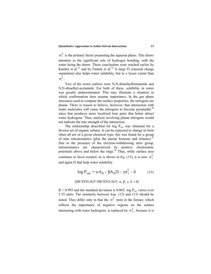
Quantitative Approaches to Solute-Solvent Interactions 13
2 is the primary factor promoting the aqueous phase. This draws
attention to the significant role of hydrogen bonding, with thewater being the donor. These conclusions were reached earlier byKamlet et al.51 and by Famini et al.52 A large (internal chargeseparation) also helps water solubility, but to a lesser extent than
2 .
Two of the worst outliers were N,N-dimethylformamide andN,N-dimethyl-acetamide. For both of these, solubility in waterwas greatly underestimated. This may illustrate a situation inwhich conformation does assume importance. In the gas phasestructures used to compute the surface properties, the nitrogens areplanar. There is reason to believe, however, that interaction withwater molecules will cause the nitrogens to become pyramidal,48
since that produces more localized lone pairs that better attractwater hydrogens. Thus, analysis involving planar nitrogens wouldnot indicate the true strength of the interaction.
The relationship described for log Pow was obtained for adiverse set of organic solutes. It can be expected to change in formwhen all are of a given chemical type; this was found for a groupof nine nitroaromatics (plus the parent benzene and toluene).53
Due to the presence of the electron-withdrawing nitro group,nitroaromatics are characterized by positive electrostaticpotentials above and below the rings.36 Thus, while surface area
continues to favor octanol, as is shown in Eq. (13), it is now 2
and again that help water solubility.
log Pow = AS AS2
(13)
(HF/STO-5G*//HF/STO-3G*; , , , > 0)
R = 0.993 and the standard deviation is 0.065; log Pow varies over1.55 units. The similarity between Eqs. (12) and (13) should be
noted. They differ only in that the 2 term in the former, which
reflects the importance of negative regions on the solutes
interacting with water hydrogens, is replaced by 2 , because it is
Peter Politzer and Jane S. Murray14
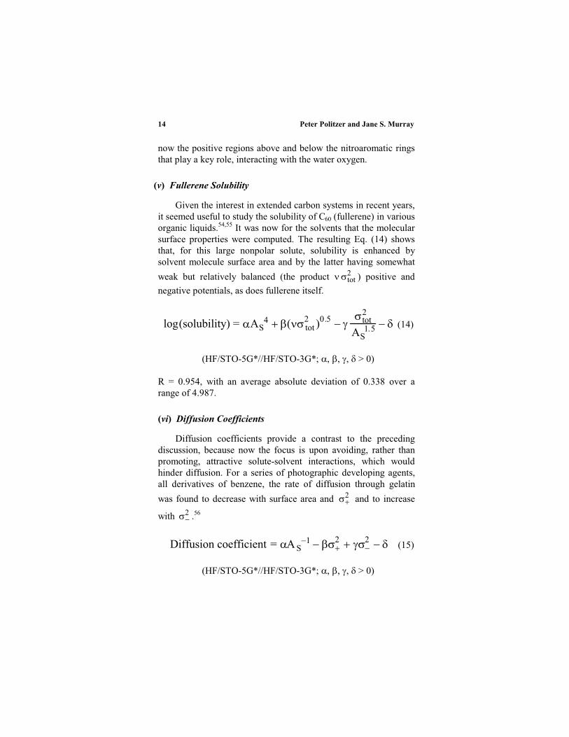
now the positive regions above and below the nitroaromatic ringsthat play a key role, interacting with the water oxygen.
(v) Fullerene Solubility
Given the interest in extended carbon systems in recent years,it seemed useful to study the solubility of C60 (fullerene) in variousorganic liquids.54,55 It was now for the solvents that the molecularsurface properties were computed. The resulting Eq. (14) showsthat, for this large nonpolar solute, solubility is enhanced bysolvent molecule surface area and by the latter having somewhat
weak but relatively balanced (the product 2tot ) positive and
negative potentials, as does fullerene itself.
log(solubility) = AS4 ( tot
2 )0.5 tot2
AS1.5 (14)
(HF/STO-5G*//HF/STO-3G*; , , , > 0)
R = 0.954, with an average absolute deviation of 0.338 over arange of 4.987.
(vi) Diffusion Coefficients
Diffusion coefficients provide a contrast to the precedingdiscussion, because now the focus is upon avoiding, rather thanpromoting, attractive solute-solvent interactions, which wouldhinder diffusion. For a series of photographic developing agents,all derivatives of benzene, the rate of diffusion through gelatin
was found to decrease with surface area and 2 and to increase
with 2 .56
Diffusion coefficient = A S1 2 2
(15)
(HF/STO-5G*//HF/STO-3G*; , , , > 0)

Quantitative Approaches to Solute-Solvent Interactions 15
R = 0.990, and the average absolute deviation is 0.065 in drygelatin (range = 1.53) and 0.6 in wet (range = 13.8). The inversedependence upon area, which promotes intermolecular attractions,
is to be expected. The roles of 2 and 2 can be attributed to the
medium, gelatin, which is a mixture of water-soluble proteins andthus contains a large number of >N C(=O) peptide linkages. Thestrongly-negative lone pair electrostatic potentials of the peptidenitrogen and oxygen will impede diffusion by attracting anypositive sites on the moving molecules, but will repel negative
sites. Diffusion is therefore favored by a high solute 2 but
hindered by a high 2 .
(vii) Solubility in Supercritical Solvents
Supercritical solutions are characterized by very low solventdensities. As a result, they possess the interesting feature thatsolubility is determined more by solute-solute than solute-solventinteractions. Thus we were able to express the solubilities ofnaphthalene and a series of indole derivatives in four differentsupercritical solvents (C2H4, C2H6, CO2 and the highly polarCHF3) in the same functional format, only the numericalcoefficients varying from one to another.57 Solute-solventinteractions do occur,58 but solubility can be represented quite
well by relating it inversely to solute surface area and 2tot ,59 large
values of which can be expected to favor solute-solute attractiveinteractions. The correlation coefficients were 0.940 and 0.921 fortwo different pressures. An interesting application of thesefindings was in identifying realistic simulants of highly toxiccompounds, to be used in investigating the proposed disposal ofthe latter through supercritical oxidation.60
(viii) Solvent Effects Upon Chemical Reactions
Gholami and Talebi have recently demonstrated that the GIPFtechnique can be utilized in analyzing the effects of solvents uponchemical reactions.61 They focused upon the Diels-Alder reactionbetween cyclopentadiene and menthyl acrylate in 15 different
Peter Politzer and Jane S. Murray16
solvents. The VS(r) quantities were computed for the solventmolecules, and expressions were developed for the rate constantsand both the endo/exo and diastereofacial selectivities in thevarious solutions. The first two properties depend upon VS,max, the
product 2tot and (inversely) molecular volume (which Gholami
and Talebi used instead of area); the last upon VS,max and . Theeffects of the solvents were interpreted in terms of their hydrogen-bond-donating ability and solvophobicity.
3. Summary
The GIPF approach is effective in correlating and predicting, withsatisfactory accuracy, various solution properties. It can also yieldinsight into the physical factors that are involved. It should bementioned that in developing the relationships that have beenpresented, our primary purpose was to demonstrate theeffectiveness of the procedure, and not necessarily to obtain thebest possible correlation. Thus it may be that those discussedcould be improved somewhat. This could also be achieved bytreating different classes of compounds separately (e.g.,hydrocarbons, alcohols, amines, etc.). We have usually tried to beas general as possible.
The GIPF technique does not address directly the interactionbetween a solute and a solvent, since one or the other is alwaysincluded only implicitly. Thus the treatment is static rather thandynamic; for instance, no account is taken of how the solute andsolvent may affect (e.g., polarize) each other. The next Sectionwill survey procedures that do, in one way or another,quantitatively involve both partners in the interaction.

Quantitative Approaches to Solute-Solvent Interactions 17
III. PROCEDURES THAT DIRECTLY ADDRESS THE
SOLUTE-SOLVENT INTERACTION
1. Discrete Molecular Models of Solvent
(i) Classical
In principle, the ideal description of a solution would be aquantum mechanical treatment of the supermolecule consisting ofrepresentative numbers of molecules of solute and solvent. Inpractice this is not presently feasible, even if only a single solutemolecule is included. In recent years, however, with the advancesin processor technology that have occurred, it has become possibleto carry out increasingly detailed molecular dynamics or MonteCarlo simulations of solutions, involving hundreds or perhapseven thousands of solvent molecules. In these, all solute-solventand solvent-solvent interactions are taken into account, at somelevel of sophistication.
Molecular dynamics and Monte Carlo methodologies differ inthat the former uses the equations of motion of classical physics todetermine the movements of the atoms and arrive at the final stateof the sytem after a lengthy series of time-steps, while the latterreaches it by random sampling of a large number of possibleconfigurations, which are accepted or rejected on the basis ofenergetic criteria.62-64 According to Orozco et al.,11 moleculardynamics is preferable for large solutes, time-dependent processesand ease of setting up the simulation, while Monte Carlo is betterfor control of temperature and pressure, and reduction ofconfigurational space.
A key to both methods is the force field that is used,65 or moreprecisely, the inter- and possibly intramolecular potentials, fromwhich can be obtained the forces acting upon the particles and thetotal energy of the system. An elementary level is to take onlysolute-solvent intermolecular interactions into account. These aretypically viewed as being electrostatic and dispersion/exchange-repulsion (sometimes denoted van der Waals); they arerepresented by Coulombic and (frequently) Lennard-Jonesexpressions:

Peter Politzer and Jane S. Murray18
612
0
RR4
R
4
1U ularintermolec
(16)
Sometimes the Buckingham potential is used, rather than theLennard-Jones:
6
0
RC)RBexp(A
R
4
1U ularintermolec
(17)
In Eqs. (16) and (17), and refer to atoms of the solute andsolvent, respectively; 0 is the permittivity of free space, Q and
Q are atomic charges, and R is the distance between atoms and . The parameters , , A , B and C can either beassigned by fitting to experimental data or can be the arithmetic orgeometric means of literature values for the individual atomtypes.10,65,66 The atomic charges are commonly determined byrequiring that they reproduce the calculated molecularelectrostatic potentials.10 In order to provide better descriptions ofthe solvent’s structure, Eqs. (16) and (17) are generally extendedto include solvent-solvent intermolecular interactions.
If it is desired to know how certain molecular properties ofthe solute (e.g., conformations) are affected by the presence of thesolvent, then it is necessary to augment Eqs. (16) and (17) byappropriate solute intramolecular potentials. These would accountfor stretching, bending and torsional motions, plus any othersdeemed significant; for typical formulations, see Kollman,10
Maple,61 and Politzer and Boyd.67 Equations (16) and (17) wouldalso be expanded to encompass solute intramolecular interactions.

Quantitative Approaches to Solute-Solvent Interactions 19
(ii) Quantum-Mechanical/Classical
The inter/intramolecular potentials that have been describedmay be viewed as classical in nature. An alternative is a hybridquantum-mechanical/classical approach, in which the solutemolecule is treated quantum-mechanically, but interactionsinvolving the solvent are handled classically. Such methods areoften labeled QM/MM, the MM reflecting the fact that classicalforce fields are utilized in molecular mechanics. An effectiveHamiltonian Heff is written for the entire solute/solvent system:
solventsoluteMMsolvent
QMsolute
eff HHHH (18)
In Eq. (18), QMsoluteH is a quantum-mechanical Hamiltonian for the
gas phase solute molecule. MMsolventH represents solvent inter- and
intramolecular interactions, and is likely to consist of termsanalogous to those in Eqs. (16) and (17). Finally, Hsolute–solvent
consists of (a) Coulombic expressions for the electrostaticinteractions between the electrons and nuclei of the solutemolecule and the atomic charges Q within the solvent molecules,and (b) Lennard-Jones or Buckingham functions for thedispersion/exchange-repulsion interactions between solute andsolvent atoms. (For more explicit depictions of Heff, see Gao9 andOrozco et al.11) Obtaining the total energy of the solute/solventsystem requires solving,
MMsolvent
solution,solutesolventsoluteQMsolutesolution,solutesystem
H
HHE
(19)
at each step of the simulation (i.e., each different configuration ofthe system), presumably by a self-consistent-field iteration. Inview of the costliness of this in terms of computer resources, it isoften preferred to use a semiempirical Hamiltonian for the solute

Peter Politzer and Jane S. Murray20
molecule, e.g., AM168 or PM3.69 Among other possibilities isWarshel’s valence bond formulation.70
(iii) Free Energy Perturbation Procedure (FEP)
Once the energy of the solute/solvent system has beendetermined, using some variant of a classical or a QM/MM forcefield, it can be used to find the free energy of solvation, which isthe property of real interest. This is given, at constant temperatureand pressure or at constant temperature and volume, respectively,by Eqs. (20) and (21):
solvationsolvationsolvation STHG (20)
solvationsolvationsolvation STEA (21)
Esolvation could be computed by,
)EE(EE solventgas,solutesystemsolvation (22)
where,
gassolute,QMsolutegassolute,gassolute, HE (23)
and Esolvent is obtained by a simulation of the pure solvent.Hsolvation would then follow by converting Esolute,gas into Hsolute,gas
at the given temperature71 and noting that for condensed phases, H E. Evaluating Ssolvation poses a problem, however, in applying
Eqs. (20) and (21).72
A widely-used alternative is the free energy perturbationtechnique (FEP),9-11,72-74 which will be discussed for the Gibbsfree energy G. It involves a thermodynamic cycle such as thefollowing, in which X and Y are two different molecules that areundergoing solvation in a particular solvent:

Quantitative Approaches to Solute-Solvent Interactions 21
The horizontal portions of this cycle consist of X mutating
reversibly into Y, in the gas phase and in solution. Since Gcycle =0, then,
Gsolvation,Y Gsolvation,X = Gmutation,solution Gmutation,gas (24)
Thus if one can determine the free energy changes for the twomutations, then Eq. (24) will yield the free energy of solvation ofY relative to that of X, Gsolvation,Y X. This is accomplishedthrough a sequence of simulations for which the force fields orHamiltonians of Xgas and Xsolution are transformed by N smallincrements into those of Ygas and Ysolution. Gmutation,gas and
Gmutation,solution then result from applying a relationship fromstatistical mechanics, which in these instances takes the forms:
1N
0i
gas,igas,1igas,mutation RT
HHexplnRTG (25)
and
1N
0i
solution,isolution,1isolution,mutation RT
HHexplnRTG
(26)
Xgas Ygas
Gmutation,gas
Xsolution Ysolution
Gsolvation,X Gsolvation,Y
Gmutation,solution

Peter Politzer and Jane S. Murray22
In Eqs. (25) and (26), the summations are over the incrementalsteps in going from X to Y in the gas phase or in solution. The Hi
are the intermediate Hamiltonians (or force fields in a classicaltreatment). Thus, Hi=0,gas = HX,gas, Hi=N,gas = HY,gas, etc. It is ofcourse desirable that the molecules X and Y be structurallysimilar, so that the perturbation of X that produces Y be small.Another option is to let Y be composed of noninteracting (dummy)atoms,75 so that its free energy of solvation is zero. Then Eq. (24)gives the absolute free energy of solvation of X:
Gsolvation,X = Gmutation,gas – Gmutation,solution (27)
(iv) Discussion of Discrete Molecular Models
Table 1 lists some relative Gsolvation calculated with classical forcefields. The average absolute deviation from experiment is 0.92kcal/mole, the largest discrepancies involving some amines andacetamides;75 some improvement was obtained for the amineswhen the force field included a term representing the polarizationof the solute.79 With a QM/MM technique, using the AM1 soluteHamiltonian,68 the average absolute deviation for the systems inTable 2 is 1.5 kcal/mole. Gao has mentioned some problems thatmay be encountered with the AM1 solute Hamiltonian, but hisoverall assessment is positive.9 In Table 3 can be seen theconsequences of two different ways of estimating atomic charges.Those derived from the molecular electrostatic potentials areclearly more effective than the Mulliken81 in this instance.
Once free energies of solvation are available, other solutionproperties can be determined, such as solute conformations, pKa
values, electrode potentials, reaction energetics, etc.9,10,82 Forexample, Reynolds applied ab initio (HF and MP2) QM/MMapproaches to computing the electrode potentials in water of agroup of quinines;83 the average absolute deviations for the moststable conformations were 0.024 (HF) and 0.033 (MP2) volts, fora range of 0.322 volts.
An important feature of QM/MM methods is that thepolarization of the solute molecule’s charge distribution by thesolvent can be evaluated, since the wave function of the former is

Quantitative Approaches to Solute-Solvent Interactions 23
Table 1
Relative Free Energies of Solvation in Water, in kcal/mole,
Obtained by Classical Discrete Molecular Solvent Methods
Gsolvation,Y Gsolvation,XX Y
Calculated Exp.Ref.
C2H6 C3H8 0.2 0.1 0.2 76CH3OH C2H6 6.9 0.1 6.9 76CH3OH (CH3)2O 3.3 3.6 10CH3OH CH3NH2 1.3 0.1 0.5 77CH3OH CH3SH 3.5 0.1 3.7 76NH3 CH3NH2 0.62 0.05 0.26 75NH3 (CH3)3N 4.36 0.05 1.07 75CH3NH2 (CH3)2NH 1.62 0.01 0.27 75(CH3)2NH (CH3)3N 2.34 0.02 1.06 75CH3C(O)NH2 CH3C(O)NHCH3 2.09 0.11 0.40 75CH3C(O)NHCH3 CH3C(O)N(CH3)2 1.05 0.02 1.53 75CH3C(O)NHCH3 CH4 11.6 0.2 12.1 76CH3SH C2H6 3.9 0.1 3.1 77CH3SH CH3CN 1.3 0.2 2.6 77(CH3)2S (CH3)2O 0.9 0.1 0.4 76
– 4.7 0.4 – 4.1 78
Table 2
Relative Free Energies Of Solvation in Water, in kcal/mole,a
Obtained by a QM/MM Discrete Molecular Solvent Method,
Using The AM1 Solute Hamiltonian. The Estimated Error
Bars for The Calculated Values Are 0.5 Kcal/Mole
Gsolvation,Y Gsolvation,XX Y
Calculated Experimental
C2H6 CH4 1.2 0.2C2H6 C6H6 0.3 2.6C2H6 H2O 8.3 8.1C2H6 CH3OH 6.2 6.9C2H6 (CH3)2O 3.6 3.7C2H6 (CH3)2CO 5.0 5.6C2H6 CH3NH2 4.0 6.4C2H6 CH3CN 3.1 5.7C2H6 CH3C(O)NHCH3 8.5 12.0C2H6 CH3CO2 80 79a Reference 84.
NH
ON OH

Peter Politzer and Jane S. Murray24
obtained in both the gas and solution phases. The energyassociated with this polarization is,9
gas,solutesolventsolutegas,solute
gas,soluteQMsolutegas,solute
solution,solutesolventsoluteQMsolutesolution,solute
.polarizsolute
H
H
HHE
(28)
The last integral in Eq. (28) represents the interaction energy ofthe unperturbed gas phase solute with the solvent. The wavefunctions solute,gas and solute,solution also permit finding the dipolemoments of the solute molecule in the gas and solution phases.
Table 3
Free Energies of Solvation in Water, in kcal/mole,aObtained
by Classical Monte Carlo Simulations Using Two Different
Atomic Charge Definitions
Gsolvation
SoluteMulliken charges
Electrostaticpotential charges
Gsolvation
(exp.)
CH3OH 9.2 0.5 4.6 0.4 5.1CH3NH2 4.2 0.5 4.3 0.5 4.6CH3CN 6.8 0.5 4.7 0.5 3.9(CH3)2O 11.3 0.5 1.4 0.5 1.9CH3SH 1.3 0.5 0.0 0.5 1.2CH3Cl 0.5 0.5 0.1 0.5 0.5C2H6 3.0 0.5 3.3 0.5 1.8CH3C(O)NH2 13.5 0.4 13.4 0.4 9.7CH3C(O)OH 10.3 0.4 8.5 0.4 6.7(CH3)2CO 5.7 0.5 3.6 0.5 3.8CH3C(O)OCH3 10.7 0.5 5.3 0.5 3.3C6H6 8.2 0.4 0.4 0.4 0.8pyridine 10.7 0.4 4.9 0.4 4.7Ave. abs.
deviation
from exp.
4.0 1.1
a Reference 80.
Quantitative Approaches to Solute-Solvent Interactions 25
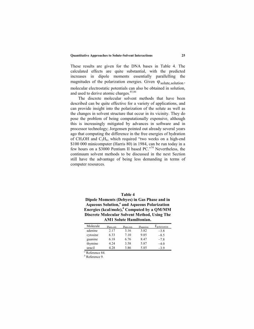
These results are given for the DNA bases in Table 4. Thecalculated effects are quite substantial, with the predictedincreases in dipole moments essentially parallelling themagnitudes of the polarization energies. Given solute,solution ,
molecular electrostatic potentials can also be obtained in solution,and used to derive atomic charges.85,86
The discrete molecular solvent methods that have beendescribed can be quite effective for a variety of applications, andcan provide insight into the polarization of the solute as well asthe changes in solvent structure that occur in its vicinity. They dopose the problem of being computationally expensive, althoughthis is increasingly mitigated by advances in software and inprocessor technology; Jorgensen pointed out already several yearsago that computing the difference in the free energies of hydrationof CH3OH and C2H6, which required “two weeks on a high-end$100 000 minicomputer (Harris 80) in 1984, can be run today in afew hours on a $3000 Pentium II based PC.”74 Nevertheless, thecontinuum solvent methods to be discussed in the next Sectionstill have the advantage of being less demanding in terms ofcomputer resources.
Table 4
Dipole Moments (Debyes) in Gas Phase and in
Aqueous Solution,a and Aqueous Polarization
Energies (kcal/mole),b Computed by a QM/MM
Discrete Molecular Solvent Method, Using The
AM1 Solute Hamiltonian.
Molecule gas,calc. gas,exp. aqueous Epolarization
adenine 2.17 3.16 3.82 3.8cytosine 6.33 7.10 9.85 8.5guanine 6.18 6.76 8.47 7.8thymine 4.24 3.58 5.87 4.0uracil 4.28 3.86 5.85 3.9
a Reference 84.b Reference 9.

Peter Politzer and Jane S. Murray26
2. Continuum Models of Solvent
(i) Classical Electrostatic Solvation Free Energy
Continuum models are rooted in classical electrostatics, andits applications in the analysis of the dielectric constants of polarliquids. A key relationship is Poisson’s equation,
)(D4
)(V2rr (29)
which links the electrostatic potential V(r) to the total chargedensity D(r) in a region with dielectric constant . D(r) includesboth electrons and nuclei. If D(r) = 0 in the region, then Laplace’sequation results,
0)(V2 r (30)
An early continuum treatment of solvation, associated withBorn,17 comes out of the analysis of the electrostatic workinvolved in building up a charge Q on a conducting sphere ofradius R in a medium with dielectric constant . From Poisson’sequation, it follows that the potential outside of the sphere isQ/ R. Thus the work of charging is the result of each additionalelement dq interacting with the charge q already present:87
R
Q
2
1dq
R
qW
2Q
0
ticelectrosta (31)
The electrostatic component of the free energy of solvation of thesphere is then the difference between doing this charging in avacuum ( = 1) and in the medium:
11
R2
QG
2
ticelectrosta (32)
Quantitative Approaches to Solute-Solvent Interactions 27
Equation (32) has been quite useful for treating the solvation ofmonatomic ions (Section III.5).88
Since the effect of the charge Q outside of the sphere is asthough it were located at the center, Eq. (32) can also be viewedas pertaining to a point charge (monopole) at the center of aspherical cavity. A few years later, it was extended to the case of apoint dipole of magnitude ,18-20 which can of course be a modelfor neutral polar molecules:
3
2
ticelectrostaR12
1G (33)
The continuum model of solvation has evolved from thesebeginnings. The solvent is treated as a continuous polarizablemedium, usually assumed to be homogeneous and isotropic, with auniform dielectric constant .11-16 The solute molecule creates andoccupies a cavity within this medium. The free energy of solvationis usually considered to be composed of three primarycomponents:
Gsolvation = Gelectrostatic + Gcavitation + GvdW (34)
Gelectrostatic is the free energy of the electrostatic interaction betweenthe solute molecule and the medium. This can be viewed in thefollowing manner:13 The charge distribution of the solute moleculeinduces polarization of the medium and the resulting induced field(the reaction field) in turn polarizes the molecule. This leads to anew reaction field, etc. The process continues until the workrequired to distort the solute and solvent charge distributionsbalances the free energy gained in the interaction. It can beanticipated that self-consistency will need to be established in themathematical treatment. Gcavitation is the free energy required toform the cavity, while GvdW refers to the solute-medium van derWaals interaction; as discussed in Section III.1.i, GvdW representsdispersion and exchange-repulsion effects. Equation (34) is oftenwritten with just Gdispersion instead of GvdW; it is also sometimesexpanded to include a term that accounts for changes in solvent

Peter Politzer and Jane S. Murray28
structure in the neighborhood of the cavity.13,16 However this isfrequently taken to be part of Gcavitation.
The evaluation of Gelectrostatic has received a great deal ofattention. It is clear that Eqs. (32) and (33), which are fornonpolarizable point charges and point dipoles, cannot reproducethe effect of the medium upon the solute molecule. A majorcontribution was made by Onsager, who took this molecule to be apolarizable point dipole located at the center of a sphericalcavity;20 the resulting expression is,
1
33
2
ticelectrostaR
2
12
11
R12
1G (35)
R is the radius of the cavity, and are the dipole moment andpolarizability of the solute, and the dielectric constant of thesolvent. Equation (35) does address the polarization of the solutemolecule by the reaction field, although not carrying this to self-consistency. (It is interesting that Onsager’s paper, the sixth-most-cited in the history of the Journal of the American Chemical
Society, was rejected by the Physikalische Zeitshrift, to which ithad initially been submitted.)89
While Onsager’s formula has been widely used, there havealso been numerous efforts to improve and generalize it. Anobvious matter for concern is the cavity. The results are verysensitive to its size, since Eqs. (33) and (35) contain the radiusraised to the third power. Within the spherical approximation, theradius can be obtained from the molar volume, as determined bysome empirical means, for example from the density, the molarrefraction, polarizability, gas viscosity, etc.90 However thevolumes obtained by such methods can differ considerably. Theshape of the cavity is also an important issue. Ideally, it should bethat of the molecule, and the latter should completely fill thecavity. Even if the second condition is not satisfied, as by a pointdipole, at least the shape of the cavity should be more realistic;most molecules are not well represented by spheres. There wasaccordingly, already some time ago, considerable interest inprogressing to more suitable cavities, such as spheroids91,92 andellipsoids,93 using appropriate coordinate systems. Such shapes
Quantitative Approaches to Solute-Solvent Interactions 29
still permit analytical solutions of Laplace’s equation, which wasinvoked for point dipoles. With increasing computing power, andfollowing Huron and Claverie’s treatment of the mathematicalproblem,94 more accurate irregular (molecular) cavities came intouse, formed by overlapping spheres centered, for example, on thenuclei or chemical groups of the solute molecule, perhaps withvan der Waals or some other appropriate radii. A seeminglyreasonable approach would be to use an outer contour of thesolute molecule’s electronic density, as is done in the GIPFmethod (Section II.1). It has been found, however, that this is noteffective in the present context.16,95 A summary and a partiallisting of some of the different cavity treatments have been givenby Tomasi and Persico.12
Improvements have also been made in expressing thepolarizing potential of the solute molecule. For a neutral molecule,the dipole term reflected in Eqs. (33) and (35) is just the first inthe multipole expansion of the potential. The inclusion of moreterms (which allows nonpolar molecules to be treated) was carriedout already by Kirkwood,19 and by others since that time, e.g.,Rivail and Rinaldi and their colleagues,96,97 whether through one-center or multi-center expansions.12-14,98 A variant of this, thegeneralized Born model, invokes distributed monopoles,99-101
centered on the nuclei of the solute molecule, and applies the Bornformula, Eq. (32). The atomic charges can be computed quantum-mechanically, for example from the molecular electrostaticpotential,10 or they can be viewed as parameters and assigned byfitting to experimental data or from some standard source, such asJorgensen and Tirado-Rives.102
The procedures that have been mentioned have focused uponEqs. (32), (33) and (35), and have sought to depict morerealistically the cavity and the polarizing effect of the solutemolecule. The reverse polarization of the latter by the reactionfield has often not been taken into account.12 A technique thatformulates Gelectrostatic in a different manner is the polarizablecontinuum model (PCM).12,103,104 This represents the reaction fieldas coming from an apparent surface charge, a charge distribution
(r) spread over the cavity surface, which is determined bysolving Poisson’s equation. (r) gives rise to a potential V (r),

Peter Politzer and Jane S. Murray30
S
d)()(V
rr
rrr (36)
where the integration is over the cavity surface. Then Gelectrostatic
can be written either as (a) the work associated with building upthis charge in the presence of the electrostatic potential due to thesolute, Vsolute(r), a process mediated by the factor ,87
rrr
rrr
d)()(V2
1
dd)()(VG
solute
1
0
soluteticelectrosta(37)
or (b) the work of creating the total charge distribution of thesolute molecule, Dsolute(r), in the presence of V (r):
rrr
rrr
d)(D)(V2
1
dd)(D)(VG
solute
solute
1
0
ticelectrosta(38)
Since Vsolute produces (r),12,103,104 and the resulting V (r)polarizes Dsolute(r), thereby giving rise to a new Vsolute, it is clearthat an iterative process could be implemented.105,106
(ii) Quantum-Mechanical Electrostatic Solvation Free Energy
The emphasis thus far has been upon classical approaches toevaluating Gelectrostatic (although quantum-mechanical methodsmight be used in some instances to obtain atomic charges or solutemolecule electronic densities.) However continuum models lendthemselves very well to quantum-mechanical treatments of solute-solvent interactions, and have indeed been incorporated intoseveral standard codes, such as the Gaussian series.29 Gelectrostatic isnow given by,
Quantitative Approaches to Solute-Solvent Interactions 31
gas,soluteQMsolutegas,solute
cavity,soluteRQMsolutecavity,soluteticelectrosta
H
VHG(39)
in which QMsoluteH is again the Hamiltonian for the gas phase solute
molecule and VR is the perturbation operator corresponding to thesolvent (i.e continuum) reaction field. The fact that VR depends on
solute,cavity imposes the requirement of self-consistency, as wasalready mentioned. The methods based on Eq. (39) are thereforelabeled SCRF (self-consistent reaction field). Thus, quantum-mechanically, the polarization of the solute molecule can be fullydescribed. Since only the solute molecule is considered explicitlyin Eq. (39), it is assumed to be acceptable to neglect any errorassociated with not converting the two energies in Eq. (39) to freeenergies.
The form of VR is generally related to one of the classicalprocedures that have been discussed.11-14,107 There has beenextensive use of truncated multipole expansions of both the solutemolecule’s charge distribution and the potential associated withthe reaction field, the latter being expressed in terms of the former.Such procedures were pioneered by Rivail, Rinaldi et al.14,108-110 atboth semi-empirical and ab initio levels, initially for spherical andellipsoidal cavities but later extended to irregular molecularshapes.14,111,112 Both one-center and multi-center expansions havebeen utilized. An interesting comparison of these was given byRivail and Rinaldi.14 For formamide, at the Hartree-Fock 6-31G*level, one-, three- and six-center treatments all gave essentially thesame Gelectrostatic ( 9.13, 9.11 and 9.13 kcal/mole, respectively).For one center, the first-order (dipolar) term is the largest, 7.82kcal/mole, but even the fifth-order is still significant, 0.48kcal/mole. For three centers, third-order is sufficient to give 9.17kcal/mole, while with six centers, second-order already produces
9.14 kcal/mole. The rate of convergence can also depend uponcavity shape; for n-propylamine, for instance, it was much morerapid in an ellipsoid than in a sphere.96 For further discussion ofconvergence issues, see Tomasi and Persico12 and Cramer andTruhlar.13,16

Peter Politzer and Jane S. Murray32
The generalized Born model (GBM) can be regarded as aspecial case of the preceding procedures; the reaction field isexpressed in terms of a multi-center monopole representation ofthe solute molecule, using the Born formula, Eq. (32).13,16,113-115
The centers are the atomic nuclei. The results are quite sensitive tothe method used to calculate the atomic charges; Cramer andTruhlar, who have applied the GBM approach extensively13,16,107
use their Class IV charges for this purpose.16,107,116 Varioustechniques have been utilized to determine the radii.16,95,101,107
It is relatively straightforward to implement the polarizablecontinuum model (PCM) via Eq. (39).11,12,105,117 The potential ofthe reaction field, V (r), is due to the ostensible (virtual) chargedistribution (r) on the cavity surface, which in turn is related tothe potential Vsolute(r) that arises from the nuclei and electrons ofthe solute molecule, Eq. (2). Since the latter is likely to be furtherpolarized by V (r), thus affecting Vsolute(r), iteration to self-consistency is needed,105,106 as already has been pointed out.(However Montagnani and Tomasi suggest that this often has littlepractical consequence.)118
In Table 5 are compared values of Gelectrostatic predicted bythese quantum-mechanical SCRF versions of the multipoleexpansion, GBM and PCM procedures.107 The solvent was takento have = 80 (for water, = 80.20 at 20 C),119 and molecularcavities were used. The computational level was HF/6-31G*. Themultipole expansion Gsolvation tends to be smaller in magnitude thanthe GBM, and the PCM larger. The average absolute differencesare 1.2 and 3.0 kcal/mole, respectively, although the latter woulddiminish to 2.2 kcal/mole if cytosine and guanine were notincluded. Curutchet et al. examine in detail the effects of usingvarious atomic radii in establishing the cavities.107 Barone et al.have also discussed this issue, and given a set of rules fordetermining atomic radii which, in a PCM treatment of hydration,decreased the mean errors in Ghydration for 43 neutral moleculesfrom 1.60 (Pauling radii)119 and 0.91 (isodensity contour, (r) =0.004 au) to 0.16 kcal/mole.95 For molecular ions, theimprovement was from 4.70 (Pauling radii) to 1.04 kcal/mole, fora range of 52 to 107 kcal/mole.

Quantitative Approaches to Solute-Solvent Interactions 33
Table 5
Values of Gelectrostatic Predicted by Three Quantum-
Mechanical SCRF Methods, in kcal/mole.aThe
Solvent Has = 80.
Method Solute Multipole
expansionGBM PCM
CH3F 1.9 3.5 3.2CHCl3 2.1 1.1 1.9C6H5SH 2.9 2.4 4.3CH3C(O)OCH3 3.8 5.5 6.8CH3CH2NO2 5.7 5.6 8.3(CH3)2CO 4.2 5.7 7.5CH3CN 5.5 8.1 7.4C6H5CHO 4.7 5.8 8.0CH3NH2 3.1 1.7 6.1CH3OH 3.5 3.8 6.8C6H5OH 4.7 4.5 7.0CH3C(O)OH 4.8 6.5 9.5CH3C(O)NH2 7.1 8.6 12.8cytosine 14.8 16.6 23.6guanine 16.7 17.6 27.5
a Reference 107.
(iii) Cavitation and van der Waals Solvation Free Energies
Gcavitation and GvdW are sometimes labeled as nonpolar, first-solvation-shell or short-range contributions to Gsolvation. They are,in general, of the same order of magnitude as Gelectrostatic, but sincethey have opposite signs (Gcavitation > 0, GvdW < 0), they partiallycancel, so that for polar solutes, normally
vdWcavitationticelectrosta GGG . This will be seen in data to be
presented in the next Section.Various approaches to evaluating Gcavitation and GvdW have been
proposed; for overviews, see Tomasi and Persico12and Cramer andTruhlar.16 It seems reasonable to relate Gcavitation to the area of thecavity and the surface tension of the solvent, as was suggested byUhlig.120 An observation made by Hermann indicated that thiscould be extended to include GvdW as well; he showed that the freeenergies of hydration of a group of saturated hydrocarbonscorrelate linearly with their solvent-accessible surface areas
Peter Politzer and Jane S. Murray34
(SA).121 If one assumes that Gelectrostatic is negligible forhydrocarbons, then Hermann’s finding could be interpreted asimplying that, approximately,
)SA(GG vdWcavitation (40)
While Eq. (41) has had some success.101,122 what is now widelyused is a version that is specific to each individual atom:107,123,124
ii
ivdWcavitation )SA(GG (41)
In Eq. (41), (SA)i is the solvent accessible surface area of atom
i. The parameters i and are assigned by fitting to
experimental Gsolvation; this has the added benefit, as shall beseen, of helping to compensate for any systematic errors inGelectrostatic. Some researchers prefer to treat Gcavitation and GvdW
separately,107,125-127 perhaps utilizing a relation-ship analogous toEq. (41) for either Gcavitation or GvdW, in combination with variantssuch as the Claverie-Pierotti expression for Gcavitation
128 or theFloris-Tomasi for GvdW.129,130
(iv) Discussion of Continuum Models
Table 6 lists computed Gcavitation + GvdW and also Gsolvation fora group of solutes in a solvent with = 80, using molecularcavities. This table complements Table 5, which gave thecorresponding Gelectrostatic. The multipole expansion and GBMGcavitation + GvdW were obtained from Eq. (41) (but with differentparameters) while the PCM work used Eq. (41) for GvdW but theClaverie-Pierotti Gcavitation.
128 The Gsolvation can be compared tothe experimental free energies of hydration of these solutes, sincewater has = 80.20 at 20 C.119
Several notable points are brought out by Table 6:
1. In view of the approximations associated with thecalculations, the results—by all three procedures—are

Ta
ble
6
Va
lues
of
Gca
vit
ati
on
+ G
vd
W a
nd
G
solv
ati
on P
red
icte
d b
y T
hre
e Q
ua
ntu
m-M
ech
an
ica
l S
CR
F
Met
ho
ds,
in
kca
l/m
ole
.aT
he
So
lven
t H
as
= 8
0.
Mul
tipl
e ex
pans
ion
GB
MPC
MSo
lute
Gca
v +
Gvd
WG
solv
Gca
v +
Gvd
WG
solv
Gca
v +
Gvd
WG
solv
Ghy
dr
(exp
.)
CH
2F—
—2.
5–1
.01.
9–1
.3–0
.2
CH
Cl 3
——
0.4
–0.7
1.4
–0.5
–1.1
C6H
5SH
——
–0.1
–2.5
2.8
–1.5
–2.6
CH
3C(O
)OC
H3
0.1
–3.7
1.9
–3.6
4.1
–2.7
–3.3
CH
3CH
2NO
2—
—1.
4–4
.24.
8–3
.5–3
.7
(CH
3)2C
O
–0.
2–4
.41.
5–4
.23.
4–4
.1–3
.9
CH
3CN
1.5
–4.0
2.6
–5.5
3.9
–3.5
–3.9
C6H
5CH
O—
—1.
0–4
.83.
2–4
.8–4
.0
CH
3NH
2
–1.
9–5
.0–2
.7–4
.41.
4–4
.7–4
.6
CH
3OH
–
1.4
–4.9
–1.5
–5.3
1.1
–5.7
–5.1
C6H
5OH
——
–2.3
–6.8
1.6
–5.4
-6.6
CH
3C(O
)OH
–
2.2
–7.0
–0.3
–6.8
2.6
–6.9
–6.7
CH
3C(O
)NH
2
–3.
0–1
0.1
–2.0
–1
0.6
3.0
–9.8
–9.7
Cyt
osin
e—
—–4
.1
–20.
72.
7
–20.
9—
Gua
nine
——
–5.9
–2
3.5
1.9
–2
5.6
—A
ve. a
bs. d
evia
tion
fro
m e
xp:
0.3
0.5
0.6
Quantitative Approaches to Solute-Solvent Interactions 35

Peter Politzer and Jane S. Murray36
quite good, with average absolute deviations fromexperiment between 0.3 and 0.6 kcal/mole.
2. The quantities Gcavitation + GvdW, because of beingparametrized by fitting to experimental Gsolvation, do helpto overcome discrepancies in Gelectrostatic. As wasmentioned in Section III.2.ii, the Gelectrostatic given by themultipole expansion and the GBM techniques differed byan average 1.2 kcal/mole, the PCM and the GBM by 3.0kcal/mole. The corresponding values for the Gsolvation inTable 6 are 0.5 and 0.7 kcal/mole. Particularly strikingare the similarities between the PCM and GBM Gsolvation
for cytosine and guanine (Table 6), in contrast to thesignificant disagreements in their Gelectrostatic (Table 5).
3. The data in Tables 5 and 6 bear out the earlier statementthat, for polar solutes, Gelectrostatic is normally larger inmagnitude than Gcavitation + GvdW, sometimes considerablyso. The only exception to this in these two tables isCH3NH2, at the GBM level.
In a very extensive test of the SM5 method (a type of GBM),Hawkins et al. found the average absolute deviation in Gsolvation tobe 0.38 kcal/mole for 260 molecular solutes in water and in 90organic solvents;131 for ions in water, it was 3.8 kcal/mole, forexperimental Gsolvation between 58 and 110 kcal/mole.Semiempirical quantum-mechanical procedures were used.
Table 7 compares free energies of hydration125 produced bythe two types of solvent models that have been presented: discretemolecular and continuum. The discrete molecular involvedclassical force field molecular dynamics (MD) and a free energyperturbation (FEP) technique whereby the solute molecule isannihilated to dummy atoms, so that absolute Ghydration areobtained; the continuum were SCRF/PCM calculations, withClaverie-Pierotti Gcavitation and Floris-Tomasi GvdW. Thecomputational level was the Hartree-Fock 6-31G*. TheSCRF/PCM results are somewhat better than the MD/FEP,although the average absolute deviation of the latter woulddecrease to 0.9 kcal/mole if CH3C(O)OH were excluded. Orozcoet al. analyze in detail the possible sources of error in the twocomputational approaches.125

Quantitative Approaches to Solute-Solvent Interactions 37
Table 7
Free Energies of Hydration Predicted by Discrete
Molecular (MD/FEP) and Continuum (SCRF/PCM)
Solvent Models, in kcal/mole.a
MethodSoluteMD/FEP SCRF/PCM Experimental
NH3 5.6 4.7 4.3H2O 5.8 6.3 6.3HCN 2.8 3.9 3.2CH3OH 3.6 4.1 5.1CH3NH2 4.4 3.3 4.6CH3C(O)OH 10.0 5.8 6.7CH3CHO 4.6 4.5 3.5(CH3)2CO 4.9 4.6 3.9Ave. abs. deviation 1.2 0.8from exp.
a Reference 125.
There have been numerous applications of continuum modelsto equilibria and reactions in solution; surveys of these andextensive listings are provided by Cramer and Truhlar.16 Otherstudies have focused upon the effects of solvents upon solutemolecular properties, such as electronic and vibrational spectra,16
dipole moments, nuclear quadrupole and spin-spin couplingconstants and circular dichroism.12
Baik and Friesner used an SCRF procedure in conjunctionwith B3LYP density functional calculations to obtain electrodepotentials for groups of aromatic molecules, metallocenes andtransition metal complexes in four different solvents;132 theaverage absolute deviation was about 0.15 volts for a range ofvalues of 3.82 volts. Saracino et al. computed pKa for a series ofcarboxylic acids with an average absolute deviation of 0.41 forpKa between 1.23 and 5.03.133
It is evident that continuum models can be quite effective, forionic solutes as well as for neutral ones. They also have theadvantage of not being highly demanding in terms of computerresources. However a problem associated with these methods isposed by so-called first-solvation-shell effects.16 One aspect of thisis the difficulty of properly accounting for specific types of solute-
Peter Politzer and Jane S. Murray38
solvent interactions that may be present, such as hydrogenbonding. Another relates to the fact that the properties of thesolvent, such as its dielectric constant and structure, are not thesame in the immediate vicinity of the solute molecule as in thebulk. To some extent, such effects can be addressed through theempirical parametrization of Gcavitation and GvdW, and through thetechniques used to assign solute atomic charges and radii; theseare important issues.95,107,134,135 An alternative is to use a hybrid orintermediate procedure, that combines features of both discretemolecular and continuum solvent models. Some examples will bediscussed in the next Section.
3. Hybrid/Intermediate Models of Solvent
One means of trying to minimize the problems mentioned at theend of the last Section is to describe the first solvation shell (orperhaps the first two) as composed of discrete molecules, withwhich the interactions are treated explicitly (for instance bymolecular dynamics or Monte Carlo simulations, or by clustercalculations) and then to use a continuum model for the remainderof the solvent.16 This makes it possible to deal more adequatelywith hydrogen bonding136,137 and other inner-solvation-shellfactors. Good results have been obtained by hybrid techniques, forions as well as for neutral solutes.138-142 A very recent example isthe approach proposed by Leontyev et al.,143,144 which wasdesigned for ions and strongly-polar molecules in polar solvents.The solute cavity is surrounded by a shell containing explicit pointcharge solvent particles; beyond this is the continuum solvent. Thecavity, shell and continuum each have a different dielectricconstant. The interaction of the solute with the shell and thecontinuum are treated separately, the first via molecular dynamicssimulation. The results for a set of polyatomic ions will bediscussed in Section III.5.iv.
A different kind of hybrid procedure was utilized byGoncalves and Stassen145 to calculate Gsolvation for a series ofsolutes in water and three organic solvents. A continuum-based(PCM) Gelectrostatic was combined with the Claverie-PierottiGcavitation and GvdW produced by molecular dynamics simulation.The resulting Gsolvation are quite good, as can be seen from the

Quantitative Approaches to Solute-Solvent Interactions 39
sample presented in Table 8, which also lists the contributions ofthe three components. In these solvents of low dielectric constant(at 20 C, = 4.806 for CHCl3 and 2.284 for benzene),119 GvdW isusually larger in magnitude than Gelectrostatic.
A solvent model that is intermediate between discretemolecules and continuum is that based upon Langevin dipoles.146-
148 The solute is surrounded by a cubic grid of polarizable pointdipoles, which represent the solvent. Each feels the electric fielddue to the solute charges and the other dipoles, and its orientationand new dipole moment in response to this field are determinediteratively using a Langevin-type formula. (The Langevin equationwas developed to treat Brownian movement.)149 A noniterativetechnique, using a position-dependent screening function, is alsopossible. The solute then interacts with the potential due to thesedipoles. Good results have been obtained for Gsolvation.
148
Another procedure that can be viewed as intermediate innature is the finite differences method (FDM).15,150-153 A three-dimensional grid is introduced into the entire system, including thesolute cavity. The dielectric constant may be uniform (althoughdifferent for solute and solvent) or position-dependent. A charge isassigned to each grid point; since the latter may not coincide withthe positions of the solute nuclei, its atomic charges must bedistributed to the neighboring grid points. A Poisson equation issolved numerically and iteratively at each grid point, using finitedifferences, to give the reaction field potential with which thesolute interacts. The accuracy of the resulting Gsolvation depends inpart upon the number of grid points; the spacing should be 0.25A–0.50 A. In the finite elements method (FEM),15,154 a grid isestablished in the solvent but the focus now is on the volumeelements that it creates; to each of these corresponds a pointcharge equal in magnitude to the charge density in the elementtimes its volume.

Ta
ble
8
Va
lues
of
Gso
lvati
on a
nd
Its
Co
mp
on
ents
in
Tw
o D
iffe
ren
t S
olv
ents
, i
n
kca
l/m
ol,
As
Pre
dic
ted
by
a H
yb
rid
Dis
cret
e M
ole
cula
r/C
on
tin
uu
m S
olv
ent
Mo
del
a
Solu
teG
cav
Gvd
WG
elec
tros
tatic
Gso
lvat
ion
Gso
lvat
ion
(exp
)
Solv
ent:
CH
Cl 3
n-oc
tane
18.5
50.
71–1
6.88
0.66
–7.5
40.
41–5
.88
0.73
–5.2
5be
nzen
e12
.05
0.43
–11.
770.
93–5
.41
0.50
–5.1
30.
20–4
.64
n-pr
opan
ol10
.94
0.73
–8.3
40.
43–6
.70
0.76
–4.1
10.
23–4
.41
1,4-
diox
ane
11.9
90.
47–1
1.36
0.85
–6.5
40.
35–5
.91
0.18
–6.2
1py
ridi
ne11
.88
0.80
–9.0
50.
92–8
.79
0.47
–5.9
70.
57–6
.45
amm
onia
5.99
0.45
–4.2
70.
55–3
.88
0.66
–2.1
70.
21–2
.41
wat
er5.
370.
35–4
.06
0.44
–4.0
90.
63–2
.79
0.49
–2.0
5
Solv
ent:
benz
ene
n-oc
tane
18.6
70.
20–1
8.92
0.44
–6.7
50.
66–6
.95
0.73
–5.3
5be
nzen
e11
.61
0.87
–7.7
70.
83–8
.84
0.65
–5.0
00.
64–4
.55
n-pr
opan
ol10
.65
0.66
–9.4
20.
85–5
.51
0.83
–4.2
80.
99–3
.87
1,4-
diox
ane
11.6
60.
19–1
0.33
0.76
–7.1
50.
46–5
.81
0.75
–5.2
1py
ridi
ne12
.31
0.55
–11.
500.
44–7
.09
0.84
–6.3
10.
88–5
.28
amm
onia
4.78
0.17
–3.8
80.
75–2
.74
0.73
–1.8
40.
41–1
.12
wat
er4.
640.
99–3
.24
0.46
–3.4
10.
25–2
.02
0.44
–1.7
1
Peter Politzer and Jane S. Murray40

Quantitative Approaches to Solute-Solvent Interactions 41
4. General Comments: Discrete Molecular and
Continuum Solvent Models
Sections III.1-III.3 have described some basic discrete molecularand continuum treatments of solute-solvent interactions. There aremany variants and refinements of these that have not beendiscussed, such as the use of effective dielectric constants66 or theimplementation of dielectric screening.155,156 For ionic solutions, itis sometimes preferred to find the reaction field potential via thePoisson-Boltzmann rather than the Poisson equation,132,157 sincethe effects of the other ions can readily be incorporated into theformer.158
The level of accuracy that can be achieved by these differentmethods may be viewed as somewhat remarkable, given theapproximations that are involved. For relatively small organicmolecules, for instance, the calculated Gsolvation is now usuallywithin less than 1 kcal/mole of the experimental value, oftenconsiderably less. Appropriate parametrization is of keyimportance. Applications to biological systems pose greaterproblems, due to the size and complexity of the molecules,66,156,159-
161 and require the use of semiempirical rather than ab initio
quantum-mechanical methods. In terms of computational expense,continuum models have the advantage over discrete molecularones, but the latter are better able to describe solvent structure andhandle first-solvation-shell effects.
5. Ionic Solvation
(i) Experimental Data
Before considering different theoretical approaches todetermining the free energies and other thermodynamic propertiesof ionic solvation, it is important to be aware of a problem on theexperimental level. There are several methods available forobtaining these quantities for electrolyte solutions, both aqueousand nonaqueous; some of these have been described by Conwayand Bockris162 and by Padova.163 For example, enthalpies ofsolvation can be found via thermodynamic cycles, free energiesfrom solubilities or galvanic cell potentials. However the results

Peter Politzer and Jane S. Murray42
pertain to the electrolyte as a whole, and there is no rigorous basisfor apportioning them between the positive and negative ions. (Itis the same problem that is encountered with respect to individualionic activity coefficients.)
Various schemes have been devised for obtaining thethermodynamic solvation properties of the separate cations andanions from the measured electrolyte values.162,163 Some havebeen based upon the concept that the solvation of small ions isprimarily electrostatic in nature and its strength is inverselyproportional to the ionic radius. Bernal and Fowler suggested thatfor a salt having positive and negative ions with similar crystalradii, the enthalpy of hydration could be divided essentiallyequally between them;164 then these could be found for other ionsfrom linear relationships between ionic Hhydration and theestimated ion-water interaction energies. Latimer et al.165 andVerwey166 proposed techniques that involved plotting thedifferences in, respectively, the free energies and enthalpies ofhydration for series of alkali halides having a common cation oranion against the inverse ionic radii. For a critique of theseapproaches, see Conway and Bockris.162 Extension to othersolvents was sometimes carried out by assuming that the ratio ofthe values for a given ion pair remains constant.167
More recently, ionic enthalpies and free energies of hydrationhave been determined relative to H+.88,168-171 This can be done, forexample, by means of appropriate thermodynamic cycles.170,171
Then by assigning the Hhydration and Ghydration of H+ on somebasis, these quantities can be evaluated for the other ion. Rashinand Honig took Hhydration (H
+) to be 262.18 kcal/mole,88 whileFlorian and Warshel assumed that Ghydration (H+) is 259.5kcal/mole.171
Table 9 compares ionic enthalpies of hydration from theBernal and Fowler,164 Latimer et al.165 and Rashin and Honig88
procedures. Given the inherent uncertainty, the latter two sets ofdata are remarkably similar, considering that they were obtained46 years apart. A number of tabulations of the thermodynamicsolvation properties of ions in various solvents have nowappeared.88,163,168-171 It is important to keep in mind, however, thatthere is a degree of arbitrariness associated with the experimental
Hsolvation and Gsolvation of individual ions.

Quantitative Approaches to Solute-Solvent Interactions 43
Table 9
Experimental Ionic Enthalpies of Hydration Obtained By
Three Different Methods, in kcal/mole
HhydrationIon
Bernal and Fowlera Latimer et al.b Rashin and Honigc
Li+ 136 121.2 125.8Na+ 114 94.6 98.5K+ 94 75.8 78.4Rb+ 87 69.2 73.4Cs+ 80 62.0 67.6F 97 122.6 119.3Cl 65 88.7 85.3Br 57 81.4 78.8I 47 72.1 69.0a Reference 164b Reference 165c Reference 88
(ii) Ionic Solvation via Discrete Molecular Solvent Models
Techniques such as those described in Section III.1, involvingmolecular dynamics or Monte Carlo simulations, have been usedextensively to study ionic solvation.84,157,172-176 A classicalintermolecular potential, e.g., Eq. (16), is often used for both ion-solvent and solvent-solvent interactions. The number of solventmolecules utilized to create the ion’s environment can have asignificant effect upon the computed energetics;172-174 an extremecase is that of F in water, for which Hhydration changed from 111to 146 kcal/mole in going from 125 to 216 water molecules.173
This was attributed to a lesser degree of solvent disruption in thelarger system. In general, 216 solvent molecules seems to bereasonable for monovalent ions, although more may be needed fordivalent ones.
Solvent reorganization can indeed be an important componentof ionic solvation. For their aqueous solutions, Chandrasekhar etal. found that this required an energy input that was, in magnitude,from 25% to 50% of the ion-solvent attraction.173
Since the solute-solvent interactions are now stronger(especially for polar solvents) than when the solute is molecular,
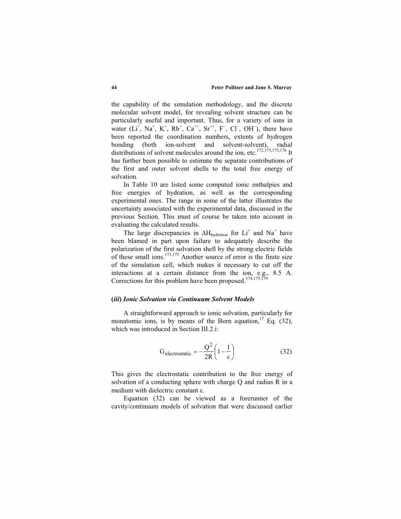
Peter Politzer and Jane S. Murray44
the capability of the simulation methodology, and the discretemolecular solvent model, for revealing solvent structure can beparticularly useful and important. Thus, for a variety of ions inwater (Li+, Na+, K+, Rb+, Ca++, Sr++, F , Cl , OH ), there havebeen reported the coordination numbers, extents of hydrogenbonding (both ion-solvent and solvent-solvent), radialdistributions of solvent molecules around the ion, etc.172,173,175,176 Ithas further been possible to estimate the separate contributions ofthe first and outer solvent shells to the total free energy ofsolvation.
In Table 10 are listed some computed ionic enthalpies andfree energies of hydration, as well as the correspondingexperimental ones. The range in some of the latter illustrates theuncertainty associated with the experimental data, discussed in theprevious Section. This must of course be taken into account inevaluating the calculated results.
The large discrepancies in Hhydration for Li+ and Na+ havebeen blamed in part upon failure to adequately describe thepolarization of the first solvation shell by the strong electric fieldsof these small ions.173,175 Another source of error is the finite sizeof the simulation cell, which makes it necessary to cut off theinteractions at a certain distance from the ion, e.g., 8.5 A.Corrections for this problem have been proposed.174,175,179
(iii) Ionic Solvation via Continuum Solvent Models
A straightforward approach to ionic solvation, particularly formonatomic ions, is by means of the Born equation,17 Eq. (32),which was introduced in Section III.2.i:
11
R2
QG
2
ticelectrosta (32)
This gives the electrostatic contribution to the free energy ofsolvation of a conducting sphere with charge Q and radius R in amedium with dielectric constant .
Equation (32) can be viewed as a forerunner of thecavity/continuum models of solvation that were discussed earlier

Quantitative Approaches to Solute-Solvent Interactions 45
(Section III.2). As was pointed out, the total free energy ofsolvation is obtained by combining Gelectrostatic with the free energyneeded to create the cavity plus that reflecting the solute-solventvan der Waals interaction:
Gsolvation = Gelectrostatic + Gcavitation + GvdW (34)
The shape and dimensions of the cavity are a key issue. In thecase of Eq. (32), it is spherical, but what value should be assignedto R? For a monatomic ion, an obvious choice is its
Table 10
Calculated (By Simulations) And Experimental Ionic
Enthalpies And Free Energies of Hydration, in kcal/mole
Hhydration GhydrationIon
Calculateda Experimental Calculatedb ExperimentalLi+ 165 4 123.0c
125.8d
130e
Na+ 126 4 96.9c
98.5d
102e
106f
76.7 89.6g
100f
F 111 4 116e
119.3d
Cl 80 5 81.4f
82e
85.3d
70.7 77h
77.7f
78i
OH 93.3 106h
110i
a Reference 173b Reference 176. The simulations were at constant volume; accordingly these are
Helmholtz free energies, Ahydration. For these aqueous solutions at 298 K,however, it is anticipated that Ahydration Ghydration
c Reference 169d Reference 88e Reference 177f Reference 168g Reference 178h Reference 170. The original values have been converted to a 1 molal ideal
solution standard state (see reference 176)iReference 171

Peter Politzer and Jane S. Murray46
crystallographically-determined ionic radius; however this wasfound to exaggerate the magnitude of Gsolvation.
165 (This may havebeen because Gcontinuum + GvdW were neglected; while thesepartially cancel, their sum is often opposite in sign to Gelectrostatic, ascan be seen in Tables 6 and 8.)
In a detailed study, Rashin and Honig concluded that crystalradii are suitable for anions but that cations should be given thecovalent radii of the corresponding neutral atoms.88 However theystill found it necessary to increase both by an empirical 7% inorder to satisfactorily reproduce experimental data. Rashin andHonig used the Gibbs-Helmholtz equation90 to convert Eq. (32)into,
T
T11
R2
QH
2
2
ticelectrosta (42)
and taking (T/ )( / T) = 1.357 for water at 298 K,180 theycalculated Helectrostatic for 28 monatomic ions. Some of theirresults are given in Table 11, along with absolute experimentalvalues obtained by assigning Hhydration for H+ to be 262.18kcal/mole.88 For all 28 ions, the calculated Helectrostatic differ fromthe absolute experimental Hhydration by, on the average, 2.5%.This overall level of agreement indicates that Eq. (42), withappropriate R, is generally effective in predicting Hhydration formonatomic ions. Rashin and Honig do warn that R for a given ionwill vary from one solvent to another, but they believe that thevalues for water should be good initial approximations for otherhydrogen-bonding solvents.
It was further pointed out by Rashin and Honig that the formof Eqs. (32) and (42) precludes significant dependence upon once it is greater than roughly 30.88 However these equations alsoemphasize the importance of long-range interactions (1/2R 16kcal/mole for R = 10 A), and the authors correctly anticipate theproblems encountered in simulations due to the limited sizes of thesystems.174,175, 179
The Born equation does not take into account the mutuallypolarizing effect that the solute and solvent have upon each other.This can be done, within the framework of continuum solvent

Quantitative Approaches to Solute-Solvent Interactions 47
models, by means of self-consistent reaction fields, at bothclassical and quantum mechanical levels. Such methods, forexample the polarizable continuum and the generalized Bornmodels (PCM and GBM) were described in Section III.2.Variations of these techniques have been applied to numerousmonatomic and polyatomic ions.95, 101, 131, 157
Table 11
Ionic Helectrostatic Obtained with
The Born Equation In The
Form of Eq. (42) Compared To
Experimental Hhydration, In
kcal/molea
Ion Helectrostatic,Eq. (42)
Hhydration,experimental
Li+ 126.7 125.8Na+ 99.3 98.5K+ 76.8 78.4Rb+ 72.2 73.4Cs+ 66.3 67.6Mg+2 458.4 462.4Ca+2 358.3 383.6Sr+2 324.7 348.3Ba+2 314.8 314.3Al+3 1122.7 1118.1Ga+3 1122.1 1124.1In+3 935.1 986.4Sc+3 974.1 939.8Cu+ 133.2 143.5Cu+2 532.8 504.5Zn+2 498.7 491.6Ag+ 116.3 115.1Cd+2 442.1 434.6Hg+2 432.9 439.4F 117.2 119.3Cl 86.1 85.3Br 79.9 78.8I 71.2 69.0S 2 338.8 325.0
a Reference 88
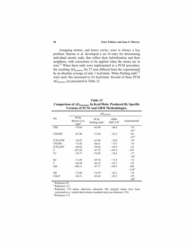
Peter Politzer and Jane S. Murray48
Assigning atomic, and hence cavity, sizes is always a keyproblem. Barone et al. developed a set of rules for determiningindividual atomic radii, that reflect their hybridization and theirneighbors, with corrections to be applied when the atoms are inions.95 When these radii were implemented in a PCM procedure,the resulting Ghydration for 27 ions differed from the experimentalby an absolute average of only 1 kcal/mole. When Pauling radii119
were used, this increased to 4.6 kcal/mole. Several of these PCMGhydration are presented in Table 12.
Table 12
Comparison of Ghydration, In Kcal/Mole, Produced By Specific
Versions of PCM And GBM Methodologies.
Ghydration
Ion PCM,Barone et al.
radiia
PCM,Pauling radiia
GBM,SM5.2 Rb Experimentalc
NH4+ 79.84 85.09 88.6 79
81d
CH3OH2+ 87.40 77.04 83.3 85
87d
(CH3)2OH+ 70.47 63.96 70.0 70CH3SH2
+ 75.56 66.41 73.5 74(CH3)2SH+ 60.82 58.64 66.9 61F 107.02 97.35 107.8 107Cl 76.77 76.05 76.9 77
78d
Br 71.89 69.76 71.8 72I 64.28 66.14 63.1 63OH 108.13 97.77 109.3 106
110d
SH 73.00 74.39 82.3 76CH3O 94.31 82.64 82.3 95
98d
a Reference 95b Reference 131c Reference 170 unless otherwise indicated. The original values have been
converted to a 1 molal ideal solution standard state (see reference 176)d Reference 171
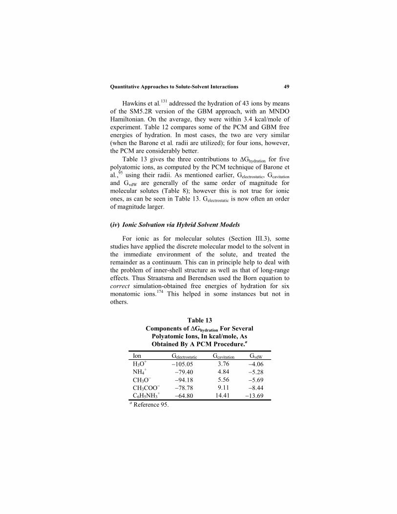
Quantitative Approaches to Solute-Solvent Interactions 49
Hawkins et al.131 addressed the hydration of 43 ions by meansof the SM5.2R version of the GBM approach, with an MNDOHamiltonian. On the average, they were within 3.4 kcal/mole ofexperiment. Table 12 compares some of the PCM and GBM freeenergies of hydration. In most cases, the two are very similar(when the Barone et al. radii are utilized); for four ions, however,the PCM are considerably better.
Table 13 gives the three contributions to Ghydration for fivepolyatomic ions, as computed by the PCM technique of Barone etal.,95 using their radii. As mentioned earlier, Gelectrostatic, Gcavitation
and GvdW are generally of the same order of magnitude formolecular solutes (Table 8); however this is not true for ionicones, as can be seen in Table 13. Gelectrostatic is now often an orderof magnitude larger.
(iv) Ionic Solvation via Hybrid Solvent Models
For ionic as for molecular solutes (Section III.3), somestudies have applied the discrete molecular model to the solvent inthe immediate environment of the solute, and treated theremainder as a continuum. This can in principle help to deal withthe problem of inner-shell structure as well as that of long-rangeeffects. Thus Straatsma and Berendsen used the Born equation tocorrect simulation-obtained free energies of hydration for sixmonatomic ions.174 This helped in some instances but not inothers.
Table 13
Components of Ghydration For Several
Polyatomic Ions, In kcal/mole, As
Obtained By A PCM Procedure.a
Ion Gelectrostatic Gcavitation GvdW
H3O+ 105.05 3.76 4.06NH4
+ 79.40 4.84 5.28CH3O 94.18 5.56 5.69CH3COO 78.78 9.11 8.44C6H5NH3
+ 64.80 14.41 13.69a Reference 95.

Peter Politzer and Jane S. Murray50
A more elaborate hybrid method is that devised by Leontyevet al.,143,144 which was described in Section III.3. For a group ofpolyatomic cations, the computed Gelectrostatic was found to bewithin an absolute average of 1.5 kcal/mole of the experimentalvalues (the latter were extracted from measured Gsolvation);
144 forthree polyatomic anions, the deviation was 5.7 kcal/mole. (Therange was 57.1 to 100.4 kcal/mole.) It was concluded that theanions require separate parametrization.
An interesting combined use of discrete molecular andcontinuum techniques was demonstrated by Floris et al.181,182 Theyused the PCM to develop effective pair potentials and then appliedthese to molecular dynamics simulations of metal ion hydration.Another approach to such systems is to do an ab initio clustercalculation for the first hydration shell, which would typicallyinvolve four to eight water molecules, and then to depict theremainder of the solvent as a continuum. This was done bySanchez Marcos et al. for a group of five cations;183 the continuummodel was that developed by Rivail, Rinaldi et al.14,108-112 (SectionIII.2.ii). Their results are compared in Table 14 with those ofFloris et al.,139 who used a similar procedure but PCM-based. In
Table 14
Ghydration For Metal Ions, In Kcal/Mole, Computed By
Two Hybrid Discrete Molecular/Continuum Methods
GhydrationIon na
Sanchez Marcos et al.b Floris et al.c Experimentald
Li+ 4 115.9 115.0Be+2 4 557.3 545.7 574.6Mg+2 6 444.8 439.6 439.3Ca+2 6 342.4 350.6Ca+2 8 359.0 362.1Ca+2 9 358.2Ni+2 6 459.4 477.5Zn+2 6 427.1 447.1 469.2Al+3 6 1041.3 1112.4 1082.9
a n is the number of water molecules in the first hydration shell; these aretreated explicitly
b Reference 183c Reference 139d Reference 178

Quantitative Approaches to Solute-Solvent Interactions 51
the latter study, Ghydration was computed for different numbers ofwater molecules in each ion’s first hydration shell to ascertain themost stable configuration; for Ca+2, which is the largest ion in thisgroup,119 this was found to be n = 8, as is shown.
IV. LINEAR SOLVATION ENERGY RELATIONSHIPS
(LSER)
1. Empirical
Some years ago, Kamlet and Taft embarked upon a study of howsolvents influence the properties of solutes, focusing initially uponthe effects of hydrogen bonding upon electronic transitions.184,185
This led eventually to an empirical relationship between aspectroscopic property X of a given solute, e.g., the position orintensity of a peak, and certain solvent parameters, , and *:186
*sbaXX 0 (43)
X0 is the value of the property in the gas phase. (In practice, X andX0 are often the logarithm of the property in question.) Theparameters and are measures of a solvent’s ability to donateand accept hydrogen bonds, respectively, and * is an index of itspolarity/polarizability. They were initially assigned on the basis ofultraviolet spectral shifts of certain dyes in a variety of solvents,and hence were labeled solvatochromic parameters.186-188
The parameters and indicate the capacity of a solvent todonate or accept a hydrogen bond from a solute, i.e., the solvent’shydrogen bond acidity or basicity. * is intended to reflect van derWaals-type solute-solvent interactions (dipolar, dispersion,exchange-repulsion, etc.). Equation (43) was subsequentlyexpanded to include a term representing the need to create a cavityfor the solute (and thus to interrupt solvent-solventinteractions).188 For this purpose was used the Hildebrandsolubility parameter, , which is defined as the square root of thesolvent’s energy of vaporization per unit volume.189 Thus Eq. (43)becomes,190

Peter Politzer and Jane S. Murray52
X = X0 + a + b + s * + h 2 (44)
(In earlier papers, entered to the first power.)188
While the original applications of the solvatochromicequations, Eqs. (43) and (44), were to correlating ultraviolet,visible and infrared spectral features of solutes, Kamlet, Taft et al.found that they were effective for numerous other properties aswell, including reaction rate constants, enthalpies and freeenergies of solvation, enthalpies and free energies of complexformation, equilibrium constants, NMR shifts and couplingconstants, partition coefficients, etc.188,191 In many instances, onlyone or two of the parameters in Eqs. (43) and (44) were required.For example, the rate constant for the reaction of tri-n-propylamine with methyl iodide in 44 organic solvents can becorrelated with * alone with R = 0.981.192 For the Gsolvation of t-butylchloride, 2-butanone and nitromethane in various organicsolvents, expressed in terms of and *, R = 0.959, 0.924 and0.991.193 For the nonpolar solute n-octane in aliphatichydrocarbons, suffices to give Gsolvation with R = 0.974.188 Sincemany of the correlations that have been established reflect freeenergies in solution, they are known collectively as linear freeenergy or linear solvation energy relationships (LFER or LSER).
The success of Eqs. (43) and (44) in describing how a givenproperty of a particular solute is affected by different solventssuggested that an analogous approach might be feasible forshowing how a property changes from one solute to another in agiven solvent. Accordingly, Abraham et al. developed soluteparameters that are counterparts to the solvents’ , and *;194-200
they were designated as H2 , H
2 and *2 (sometimes written as
H2 ). These have been incorporated in a number of
relationships,198-201 of the general form,
X = + a H2 + b H
2 + s *2 + rR2 + vVx (45)
In Eq. (45), is a constant. R2 is related to the solute’s molarrefraction198 and can be viewed as a correction to thepolarity/polarizability term, analogous to one that has sometimes

Quantitative Approaches to Solute-Solvent Interactions 53
been included in Eqs. (43) and (44).186-188 Vx is a solute’scharacteristic molecular volume,202,203 which can readily becalculated from its molecular structure. An equation that combinesboth solute and solvent parameters has also been used onoccasion,199,201,204 for example,
X = + a 1H2 + b 1
H2 + s *
1*2 + vVx (46)
The subscripts 1 and 2 refer to solvent and solute, respectively.Relationships such as Eqs. (45) and (46) have been utilized
extensively in correlating solubility properties (such as gas/liquidand liquid/liquid partition coefficients), retention volumes ingas/solid chromatography, capacity factors in high-pressure liquidchromatography, etc.199,200 For instance, gas/liquid partitioncoefficients for each of 35 different liquid stationary phases wererepresented with R 0.985.205 Other applications have been inbiochemical and pharmacological areas,199,200 e.g., enzymeinhibition and pollutant effects.
The LSER that have been discussed have had considerablesuccess in correlating a variety of properties, which means thatthey have, in general, a good predictive capability. They alsoprovide insight, through the magnitudes of the coefficients in Eqs.(43)–(46), into the factors that play important roles in specifictypes of solute-solvent interactions. Since the parameters areexperimentally-derived, however, predictions can be made onlyfor existing compounds. (Hickey and Passino-Reader havesuggested rules for estimating the LSER parameters.)206 Therehave accordingly been proposed a number of procedures forcorrelating and predicting solution properties from parameters thatcan be obtained theoretically or computationally; briefdescriptions of some of these have been given by Famini andWilson207 and Murray et al.208 The next Section will focus uponone of these approaches, which is patterned after the LSER ofKamlet, Taft, Abraham et al., Eqs. (43)–(46).
2. Theoretical
Famini, Wilson et al. have correlated a wide array of physical,chemical and biological properties by means of theoretical linear

Peter Politzer and Jane S. Murray54
solvation energy relationships (TLSER).207,209 These weredesigned to be theoretical analogs of the empirical LSER, Eqs.(43)–(46). Thus, for a given solute in a series of solvents,
X = X0 + a A1 + b B1 + c 1q + d 1q + s 1*
+ h 21 (47)
while for a series of solutes in one solvent,
X = + a A2 + b B2 + c 2q + d 2q + s *2 + v 2mcV (48)
and finally the combined form,
X = + a A1 B2 + b B1 A2 + cq1 q2
+ d 1q 2q + s *1
*2 + h 2
1 mc2V (49)
In Eqs. (47)–(49), the subscripts 1 and 2 are again used to indicatesolvent and solute. Hydrogen-bond-donating ability is nowexpressed in terms of a covalent and an electrostatic contribution,
A and q+; A is the magnitude of the difference between theenergies of the lowest unoccupied molecular orbital (LUMO) ofthe molecule and the highest occupied (HOMO) of water, while q+
is the atomic charge of the most positive hydrogen. For hydrogen-bond-accepting ability, B is the magnitude of the differencebetween the molecule’s HOMO and water’s LUMO, with q– theabsolute value of the most negative atomic charge. (Water is usedsimply as a reference system.) The polarity/polarizability index,
*, is related to the molecule’s polarizabilty per unit volume, andVmc is its van der Waals volume. is again the Hildebrandparameter. The quantum-mechanical calculations are carried outwith semiempirical methods.
These TLSER have been used to develop a large number ofcorrelations,207,209 particularly involving different sorts ofpharmacological activities. For example, acetylcholinesterase
inhibition by 44 alkylammonium ions correlates with 2q , *2 and
Vmc2 with R = 0.958.209 The toxicities of a group of 28 industrial

Quantitative Approaches to Solute-Solvent Interactions 55
pollutants can be expressed in terms of B2,*2 and Vmc2 with R =
0.992.207
V. DISCUSSION AND SUMMARY
This Chapter has outlined several different approaches to thecomputational determination of solution properties. Two of theseaddress solute-solvent interactions directly, either treating theeffects of individual solvent molecules upon the solute explicitlyor by means of a reaction field due to a continuum model of thesolvent. The other procedures establish correlations betweenproperties of interest and certain features of the solute and/orsolvent molecules. There are empirical elements in all of thesemethods, even the seemingly more rigorous ones, such as theparameters in the molecular dynamics/Monte Carlo intermolecularpotentials, Eqs. (16) and (17), or in the continuum model’sGcavitation and GvdW, Eqs. (40) and (41), etc.
The correlation-based techniques can achieve as high levelsof accuracy as the direct-interaction ones; for example, the GIPF
Ghydration have average absolute deviations from experiment, 0.27kcal/mole (Section II.2.iii), as good or better than the SCRF
Ghydration in Table 6. However the GIPF, LSER and TLSERcannot describe the effects of the solute and solvent upon eachother, such as polarization of the former and disruption of thestructure of the latter.
The GIPF, LSER and TLSER methodologies have incommon that they rely on correlations established fromexperimental databases. They differ fundamentally, however, inthe natures of the parameters used for this purpose. Those in theLSER and TLSER were intended specifically to reflect certainaspects of solute-solvent interactions, i.e., hydrogen-bond-donating and –accepting, polarity/polarizability and cavitation. Incontrast, the GIPF quantities, Eq. (9), were designed simply toquantitatively characterize, as well as possible, the features ofmolecular surface electrostatic potentials. While there are goodcorrelations between some of the GIPF and LSER/TLSERparameters,208 this is a significant conceptual distinction between

Peter Politzer and Jane S. Murray56
them, and between GIPF and quantitative structure-propertyrelationships (QSPR) in general.
If one’s interest is solely in predicting a particular solutionproperty, then the GIPF, LSER and TLSER approaches are fast,inexpensive and can be quite accurate, provided that correlationsdeveloped from appropriate databases are available. Even if theseremain to be established, that can be done in a relatively short time(~ 1 week) and the resulting relationship, if GIPF or TLSER, canbe used even for compounds that may not yet have beensynthesized. However if a more complete picture of the interactionis desired, then a discrete molecular or continuum (orhybrid/intermediate) procedure should be used. The continuumtechniques are faster, less computationally demanding, and, atleast for Gsolvation, appear to be slightly more accurate. For ionicsolutes, they may be better able to treat long-range effects. If first-solvation-shell effects are expected to be especially important, orif the disruption of solvent structure is to be characterized, then adiscrete molecular solvent model may be preferred. The appeal ofthe hybrid methods is of course that they can, at least in principle,combine the strengths of both of the others.
ACKNOWLEDGEMENT
We greatly appreciate the support of the Office of NavalResearch, Contract No. N00014-99-1-0393 and Project OfficerDr. Judah M. Goldwasser.
REFERENCES
1.H. Hellmann, Einfuhrung in die Quantenchemie, Franz Deuticke, Leipzig, 1937.2R. P. Feynman, Phys. Rev. 56 (1939) 340.3J. O. Hirschfelder, C. F. Curtiss and R. B. Bird, Molecular Theory of Gases and
Liquids, Wiley, New York, 1954.4J. O. Hirschfelder and W. J. Meath, Adv. Chem. Phys. 12 (1967) 3.5G. Chalasinski and M. M. Szczesniak, Chem. Rev. 100 (2000) 4227.6A. K. Rappe and E. R. Bernstein, J. Phys. Chem. A 104 (2000) 6117.7B. Jeziorski, R. Moszynski and K. Szalewicz, Chem. Rev. 94 (1994) 1887.8O. Engkvist, P.-O. Astrand and G. Karlstrom, Chem. Rev. 100 (2000) 4087.9J. Gao, Acc. Chem. Res. 29 (1996) 298.10P. A. Kollman, Acc. Chem. Res. 29 (1996) 461.

Quantitative Approaches to Solute-Solvent Interactions 57
11M. Orozco, C. Alhambra, X. Barril, J. M. Lopez, M. A. Busquets and F. J.Luque, J. Mol. Mod. 2 (1996) 1.
12J. Tomasi and M. Persico, Chem. Rev. 94 (1994) 2027.13C. J. Cramer and D. G. Truhlar, in Quantitative Treatments of Solute/Solvent
Interactions, Ed. by P. Politzer and J. S. Murray, Elsevier, Amsterdam, 1994,Ch. 2.
14J.-L. Rivail and D. Rinaldi, in Computational Chemistry: Reviews of Current
Trends, Vol. 1, Ed. by J. Leszczynski, World Scientific, Singapore, 1996, Ch. 4.15J. Tomasi and B. Mennucci, in Encyclopedia of Computational Chemistry, Vol.
4, Ed. by P.von R. Schleyer, Wiley, New York, 1998, pp. 2547-2560.16C. J. Cramer and D. G. Truhlar, Chem. Rev. 99 (1999) 2161.17M. Born, Z. Physik 1 (1920) 45.18R. P. Bell, Trans. Faraday Soc. 27 (1931) 797.19J. G. Kirkwood, J. Chem. Phys. 2 (1934) 351.20L. Onsager, J. Am. Chem. Soc. 58 (1936) 1486.21I. Langmuir, Colloid Symp. Monogr. 3 (1925) 48.22F. M. Richards, Annu. Rev. Biophys. Bioeng. 6 (1977) 151.23P. K. Weiner, R. Langridge, J. M. Blaney, R. Schaefer, P. A. Kollman, Proc.
Natl. Acad. Sci. 79 (1982) 3754.24M. L. Connolly, Science, 221 (1983) 709.25M. M. Francl, R. F. Hout, Jr. and W. J. Hehre, J. Am. Chem. Soc. 106 (1984)
563.26R. F. W. Bader, M. T. Carroll, J. R. Cheeseman and C. Chang, J. Am. Chem.
Soc. 109 (1987) 7968.27P. Politzer and D. G. Truhlar (eds.), Chemical Applications of Atomic and
Molecular Electrostatic Potentials, Plenum, New York, 1981.28G. Naray-Szabo and G. G. Ferenczy, Chem. Rev. 95 (1995) 829.29M. J. Frisch, G. W. Trucks, H. B. Schlegel, G. E. Scuseria, M. A. Robb, J. R.
Cheeseman, V. G. Zakrezewski, J. A. Montgomery, R. E. Stratmann, J. C.Burant, S. Dappich, J. M. Millam, A. D. Daniels, K. N. Kudin, M. C. Strain, O.Farkas, J. Tomasi, V. Barone, M. Cossi, R. Cammi, B. Mennucci, C. Pomelli, C.Adamo, S. Clifford, J. Ochterski, G. Petersson, P. Y. Aayala, Q. Cui, K.Morokuma, D. K. Malick, A. D. Rubuck, K. Raghavachari, J. B. Foresman, J.Cioslowski, J. V. Ortiz, B. B. Stefanov, G. Liu, A. Liashenko, P. Piskorz, I.Komaromi, R. Gomperts, R. L. Martin, D. J. Fox, T. Keith, M. A. Al-Laham, C.Y. Peng, A. Nanayakkara, C. Gonzalez, M. Challacombe, P. M. W. Gill, B. G.Johnson, W. Chen, M. W. Wong, J. L. Andres, M. Head-Gordon, E. S. Replogleand J. A. Pople, Gaussian 98, Revision A.5 (Gaussian, Inc., Pittsburgh, PA,1998).
30J. S. Murray, Z. Peralta-Inga, P. Politzer, K. Ekanayake and P. LeBreton, Int. J.
Quantum Chem. 83 (2001) 245.31J. S. Murray and P. Politzer, J. Mol. Struct. (Theochem) 425 (1998) 107.32J. S. Murray and P. Politzer, in Encyclopedia of Computational Chemistry, Vol.
2, Ed. by P. von R. Schleyer, Wiley, New York, 1998, pp. 912-920.33P. Politzer and J. S. Murray, Trends Chem. Phys. 7 (1999) 157.34P. Politzer and J. S. Murray, Fluid Phase Equil. 185 (2001) 129.35T. Brinck, J. S. Murray and P. Politzer, Mol. Phys. 76 (1992) 609.36J. S. Murray, P. Lane and P. Politzer, Mol. Phys. 93 (1998) 187.

Peter Politzer and Jane S. Murray58
37J. S. Murray, T. Brinck, P. Lane, K. Paulsen and P. Politzer, J. Mol. Struct.
(Theochem) 307 (1994) 55.38J. S. Murray, T. Brinck, M. E. Grice and P. Politzer, J. Mol. Struct. (Theochem)
256 (1992) 29.39J. Allinger and N. L. Allinger, Tetrahedron 2 (1958) 64.40J. S. Murray, Z. Peralta-Inga and P. Politzer, Int. J. Quantum Chem. 75 (1999)
267.41J. S. Murray, Z. Peralta-Inga and P. Politzer, Int. J. Quantum Chem. 80 (2000)
1216.42P. Politzer and J. S. Murray, in Reviews in Computational Chemistry, Vol. 2,
Ed. by K. B. Lipkowitz and D. B.Boyd, VCH, New York, 1991, Ch. 7.43P. Politzer and K. C. Daiker, in The Force Concept in Chemistry, Ed. by B. M.
Deb, Van Nostrand Reinhold, New York, 1981, Ch. 6.44J. S. Murray and P. Politzer, J. Chem. Res. S, (1992) 110.45H. Hagelin, J. S. Murray, T. Brinck, M. Berthelot and P. Politzer, Can. J. Chem.
73 (1995) 483.46J. S. Murray, F. Abu-Awwad and P. Politzer, J. Phys. Chem. A 103 (1999) 1853.47P. Politzer, J. S. Murray and F. Abu-Awwad, Int. J. Quantum Chem. 76 (2000)
643.48J. S. Murray, Z. Peralta-Inga, P. Jin and P. Politzer, unpublished work.49C. Hansch, Acc. Chem. Res. 26 (1993) 147.50T. Brinck, J. S. Murray and P. Politzer, J. Org. Chem. 58 (1993) 7070.51M. J. Kamlet, R. M. Doherty, M. H. Abraham, Y. Marcus and R. W. Taft, J.
Phys. Chem. 92 (1988) 5244.52G. R. Famini, C. A. Penski and L. Y. Wilson, J. Phys. Org. Chem. 5 (1992) 395.53J. S. Murray, T. Brinck and P. Politzer, J. Phys. Chem. 97 (1993) 13807.54J. S. Murray, S. G. Gagarin and P. Politzer, J. Phys. Chem. 99 (1995) 12081.55P. Politzer, J. S. Murray and S. G. Gagarin, in Recent Advances in the Chemistry
and Physics of Fullerenes and Related Materials, Vol. 3, Ed. by K. M. Kadishand R. S. Ruoff, The Electrochemical Society, Pennington, NJ, 1996, pp. 45-52.
56P. Politzer, J. S. Murray and P. Flodmark, J. Phys. Chem. 100 (1996) 5538.57P. Politzer, P. Lane, J. S. Murray and T. Brinck, J. Phys. Chem. 96 (1992) 7938.58J. S. Murray, P. Lane, T. Brinck and P. Politzer, J. Phys. Chem. 97 (1993) 5144.59P. Politzer, J. S. Murray, P. Lane and T. Brinck, J. Phys. Chem. 97 (1993) 729.60P. Politzer, J. S. Murray, M. C. Concha and T. Brinck, J. Mol. Struct.
(Theochem) 281 (1993) 107.61M. R. Gholami and B. A. Talebi, J. Phys. Org. Chem. 16 (2003) 369.62M. P. Allen and D. J. Tildesley, Computer Simulations of Liquids, Clarendon
Press, Oxford, 1987.63J. M. Haile, Molecular Dynamics Simulations, Wiley, New York, 1992.64W. L. Jorgensen, in Encyclopedia of Computational Chemistry, Vol. 3, Ed. by
P. von R. Schleyer, Wiley, 1998, pp. 1754-1763.65J. R. Maple, in Encyclopedia of Computational Chemistry, Vol. 2, Ed. by P. von
R. Schleyer, Wiley, 1998, pp. 1015-1024.66P. E. Smith and B. M. Pettitt, J. Phys. Chem. 98 (1994) 9700.67P. Politzer and S. Boyd, Struct. Chem. 13 (2002) 105. 68M. J. S. Dewar, E. G. Zoebisch, E. F. Healy and J. J. P. Stewart, J. Am. Chem.
Soc. 107 (1985) 3902. 69J. J. P. Stewart, J. Comput. Chem. 10 (1989) 209, 221.

Quantitative Approaches to Solute-Solvent Interactions 59
70J. Aqvist and A. Warshel, Chem. Rev. 93 (1993) 2523. 71W. J. Hehre, L. Radom, P. von R. Schleyer and J. A. Pople, Ab Initio Molecular
Orbital Theory, Wiley, New York, 1986. 72W. F. van Gunsteren, in Computer Simulation of Biomolecular Systems, Ed. by
W. F. van Gunsteren and P. K. Weiner, ESCOM, Leiden (The Netherlands),1989, pp. 27-59.
73P. A. Kollman and K. M. Merz, Jr., Acc. Chem. Res. 23 (1990) 246. 74W. L. Jorgensen, in Encyclopedia of Computational Chemistry, Vol. 2, Ed. by
P. von R.Schleyer, Wiley, 1998, pp. 1061-1070. 75P.-Y. Morgantini and P. A. Kollman, J. Am. Chem. Soc. 117 (1995) 6057. 76W. D. Cornell, P. Cieplak, C. I. Bayly, I. R. Gould, K. M. Merz, Jr., D. M.
Ferguson, D. C. Spellmeyer, T. Fox, J. W. Caldwell and P. A. Kollman, J. Am.
Chem. Soc. 117 (1995) 5179. 77W. L. Jorgensen and J. M. Briggs, J. Am. Chem. Soc. 111 (1989) 4190. 78P. Cieplak, P. Bash, S. C. Singh and P. A. Kollman, J. Am. Chem. Soc. 109
(1987) 6283. 79E. C. Meng, J. W. Caldwell and P. A. Kollman, J. Phys. Chem. 100 (1996)
2367. 80H. A. Carlson, T. B. Nguyen, M. Orozco and W. L. Jorgensen, J. Comput.
Chem. 14 (1993) 1240. 81R. S. Mulliken, J. Chem. Phys. 23 (1955) 1833. 82W. L. Jorgensen, Acc. Chem. Res. 22 (1989) 184. 83C. A. Reynolds, J. Am. Chem. Soc. 112 (1990) 7545. 84J. Gao and X. Xia, Science 258 (1992) 631. 85J. Gao, F. J. Luque and M. Orozco, J. Chem. Phys. 98 (1993) 2975. 86T. J. Marrone, D. S. Hartsough and K. M. Merz, Jr., J. Phys. Chem. 98 (1994)
1341. 87W. R. Smythe, Static and Dynamic Electricity, McGraw-Hill, New York, 1950. 88A. A. Rashin and B. Honig, J. Phys. Chem. 89 (1985) 5588. 89Chemical & Engineering News, Nov. 17 (2003) 70. 90S. Glassstone, Text-book of Physical Chemistry, Van Nostrand, New York,
1940. 91T. G. Scholte, Physica 15 (1949) 437. 92A. D. Buckingham, Trans. Faraday Soc. 49 (1953) 881. 93F. H. Westheimer and J. G. Kirkwood, J. Chem. Phys. 6 (1938) 513. 94M. J. Huron and P. Claverie, J. Phys. Chem. 76 (1972) 2123; 78 (1974) 1853,
1862. 95V. Barone, M. Cossi and J. Tomasi, J. Chem. Phys. 107 (1997) 3210. 96J.-L. Rivail and B. Terryn, J. Chim. Phys. Physicochim. Biol. 79 (1982) 1. 97D. Rinaldi, Comput. & Chem. 6 (1982) 155. 98J. Tomasi, R. Bonaccorsi, R. Cammi and F. J. Olivares del Valle, J. Mol.
Struct. (Theochem) 234 (1991) 401. 99G. J. Hoijting, E. de Boer, P. H. van der Meij and W. P. Weijland, Rec. Trav.
Chim. Pays-Bas 75 (1956) 487.100O. Chalvet and I. Jano, Compt. Rend. Seances Acad. Sci. 259 (1964) 1867.101W. C. Still, A. Tempczyk, R. C. Hawley and T. Hendrickson, J. Am. Chem.
Soc. 112 (1990) 6127.102W. L. Jorgensen and J. Tirado-Rives, J. Am. Chem. Soc. 110 (1988) 1657.103S. Miertus and J. Tomasi, Chem. Phys. 65 (1982) 239.

Peter Politzer and Jane S. Murray60
104A. A. Rashin and K. Namboodiri, J. Phys. Chem. 91 (1987) 6003.105F. J. Luque, J. M. Bofill and M. Orozco, J. Chem. Phys. 103 (1995) 10183. See
also J. G. Angyan, J Chem. Phys. 107 1291 (1997) 1291 and F. J. Luque, J. M.Bofill and M. Orozco, J. Chem. Phys. 107 (1997) 1293.
106I. N. Levine, Quantum Chemistry, 5th ed., Prentice Hall, Upper Saddle River,NJ, 2000.
107C. Curutchet, C. J. Cramer, D. G. Truhlar, M. F. Ruiz-Lopez, D. Rinaldi, M.Orozco and F. J. Luque, J. Comput. Chem. 24 (2003) 284.
108D. Rinaldi and J.-L. Rivail, Theor. Chim. Acta 32 (1973) 57.109J.-L. Rivail and D. Rinaldi, Chem. Phys. 18 (1976) 233.110D. Rinaldi, M. F. Ruiz-Lopez and J.-L. Rivail, J. Chem. Phys. 78 (1983) 834.111V. Dillet, D. Rinaldi and J.-L. Rivail, J. Phys. Chem. 98 (1994) 5034.112V. Dillet, D. Rinaldi, J. Bertran and J.-L. Rivail, J. Chem. Phys. 104 (1996)
9437.113O. Tapia, in Quantum Theory of Chemical Reactions, Vol. II, Ed. by R. Daudel,
A. Pullman, L.Salem and A. Veillard, Reidel, Dordrecht, 1981, p. 25.114R. Constanciel and R. Contreras, Theor. Chim. Acta 65 (1984) 1.115T. Kozaki, K. Morihashi and O. Kikuchi, J. Mol. Struct. 168 (1988) 265.116J. W. Storer, D. J. Giesen, C. J. Cramer and D. G. Truhlar, J. Comput.-Aided
Mol. Design 9 (1995) 87.117S. Miertus, E. Scrocco and J. Tomasi, Chem. Phys. 55 (1981) 117.118R. Montagnani and J. Tomasi, J. Mol. Struct. (Theochem) 279 (1993) 131.119D. R. Lide (ed.), Handbook of Chemistry and Physics, 78th ed., CRC Press,
New.York, 1997.120H. H. Uhlig, J. Phys. Chem. 41 (1937) 1215.121R. B. Hermann, J. Phys. Chem. 76 (1972) 2754.122D. Sitkoff, K. A. Sharp and B. Honig, J. Phys. Chem. 98 (1994) 1978.123C. J. Cramer and D. G. Truhlar, J. Am. Chem. Soc. 113 (1991) 8305.124I. Tunon, M. F. Ruiz-Lopez, D. Rinaldi and J. Bertran, J. Comput. Chem. 17
(1996) 148.125M. Orozco, W. L. Jorgensen and F. J. Luque, J. Comput. Chem. 14 (1993)
1498.126V. Gogonea and E. Osawa, J. Mol. Struct. (Theochem) 311 (1994) 305.127M. Zacharias, J. Phys. Chem. A 107 (2003) 3000.128R. A. Pierotti, Chem. Rev. 76 (1976) 717; P. Claverie, Perspect. Quantum
Chem. Biochem. 2 (1978) 69.129F. M. Floris and J. Tomasi, J. Comput. Chem. 10 (1989) 616.130F. M. Floris, A. Tani and J. Tomasi, Chem. Phys. 169 (1993) 11.131G. D. Hawkins, C. J. Cramer and D. G. Truhlar, J. Phys. Chem. B 102 (1998)
3257.132M.-H. Baik and R. A. Friesner, J. Phys. Chem. A 106 (2002) 7407.133G. A. A. Saracino, R. Improta and V. Barone, Chem. Phys. Lett. 373 (2003)
411.134D. F. Green and B. Tidor, J. Phys. Chem. B 107 (2003) 10261.135K. N. Rankin, T. Sulea and E. O. Purisima, J. Comput. Chem. 24 (2003) 954.136E. Sanchez Marcos, B. Terryn and J.-L. Rivail, J. Phys. Chem. 89 (1985) 4695.137J. Zeng, J. S. Cram, N. S. Hush and J. R. Reimers, Chem. Phys. Lett. 206
(1993) 323.

Quantitative Approaches to Solute-Solvent Interactions 61
138E. Sanchez Marcos, R. R. Pappalardo and D. Rinaldi, J. Phys. Chem. 95 (1991)8928.
139F. M. Floris, M. Persico, A. Tani and J. Tomasi, Chem. Phys. 195 (1995) 207.140C. Aleman and S. E. Galembeck, Chem. Phys. 232 (1998) 151.141M. Brauer, M. Mosquera, J. L. Perez-Lustres and F. Rodriguez-Prieto, J. Phys.
Chem. A 102 (1998) 10736.142C. Aleman, Chem. Phys. Lett. 302 (1999) 461.143I. V. Leontyev, M. V. Vener, I. V. Rostov, M. V. Basilevsky and M. D.
Newton, J. Chem. Phys. 119 (2003) 8024.144M. V. Vener, I. V. Leontyev and M. V. Basilevsky, J. Chem. Phys. 119 (2003)
8038.145P. F. B. Goncalves and H. Stassen, J. Comput. Chem. 23 (2002) 706; 24 (2003)
1758.146A. Warshel and M. Levitt, J. Mol. Biol. 103 (1976) 227.147A. Warshel and S. T. Russell, Quantum Rev. Biophys. 17 (1984) 285.148A. Warshel and Z. T. Chu, in Structure and Reactivity in Aqueous Solution.
Characterization of Chemical and Biological Systems, Ed. by C. J. Cramer andD. G. Truhlar, ACS Symposium Series 568, American Chemical Society,Washington, DC, 1994, pp. 71-94.
149P. Langevin, Compt. Rend. Acad. Sci. Paris 146 (1908) 530.150J. Warwicker and H. C. Watson, J. Mol. Biol. 157 (1982) 671.151D. T. Edmonds, N. K. Rogers and M. J. E. Sternberg, Mol. Phys. 52 (1984)
1487.152M. K. Gilson, K. A. Sharp and B. H. Honig, J. Comput. Chem. 9 (1988) 327.153M. E. Davis and J. A. McCammon, J. Comput. Chem. 10 (1989) 387; 12
(1991) 909.154W. H. Orttung, J. Am. Chem. Soc. 100 (1978) 4369.155R. Luo, J. Moult and M. K. Gilson, J. Phys. Chem. B 101 (1997) 11226.156S. A. Hassan, F. Guarnieri and E. L. Mehler, J. Phys. Chem. B 104 (2000)
6478, 6490.157A. Jean-Charles, A. Nicholls, K. Sharp, B. Honig, A. Tempczyk, T. F.
Hendrickson and W. C. Still, J. Am. Chem. Soc. 113 (1991) 1454.158R. D. Coalson and T. L. Beck, in Encyclopedia of Computational Chemistry,
Vol. 3, Ed. by P. von R. Schleyer, Wiley, New York, 1998, pp. 2086-2100.159B. Honig, K. Sharp and A.-S. Yang, J. Phys. Chem. 97 (1993) 1101.160N. G. J. Richards, in Molecular Orbital Calculations for Biological Systems,
Ed. by A.-M. Sapse, Oxford University Press, New York, 1998, Ch. 2.161D. Bashford, in Encyclopedia of Computational Chemistry, Vol. 3, Ed. by P.
von R. Schleyer, Wiley, New York, 1998, pp. 1542-1548.162B. E. Conway and J. O’M. Bockris, in Modern Aspects of Electrochemistry,
vol. 1, Ed. by J. O’M. Bockris, Butterworths, London, 1954, Ch. 2.163J. I. Padova, in Modern Aspects of Electrochemistry, Vol. 7, Ed. by B. E.
Conway and J. O’M. Bockris, Plenum Press, New York, 1972, Ch. 1.164J. D. Bernal and R. H. Fowler, J. Chem. Phys. 1 (1933) 515.165W. M. Latimer, K. S. Pitzer and C. M. Slansky, J. Chem. Phys. 7 (1939) 108.166E. J. W. Verwey, Rec. Trav. Chim. 61 (1942) 127, 564.167K. P. Mischenko, Acta Physicochim. URSS 3 (1935) 693.168D. R. Rosseinsky, Chem. Rev. 65 (1965) 467.169J. Burgess, Metal Ions in Solution, Ellis Horwood, Chichester, UK, 1978.
Peter Politzer and Jane S. Murray62
170R. G. Pearson, J. Am Chem. Soc. 108 (1986) 6109.171J. Florian and A. Warshel, J. Phys. Chem. B 101 (1997) 5583.172M. Mezei and D. L. Beveridge, J. Chem. Phys. 74 (1981) 6902.173J. Chandrasekhar, D. C. Spellmeyer and W. L. Jorgensen, J. Am. Chem. Soc.
106 (1984) 903.174T. P. Straatsma and H. J. C. Berendsen, J. Chem. Phys. 89 (1988) 5876.175B. Jayaram, R. Fine, K. Sharp and B. Honig, J. Phys. Chem. 93 (1989) 4320.176P. B. Balbuena, K. P. Johnston and P. J. Rossky, J. Phys. Chem. 100 (1996)
2706.177J. O’M. Bockris and A. K. N. Reddy, Modern Electrochemistry, Vol. 1, Plenum
Press, New York, 1970, Ch. 2.178Y. Marcus, Ion Solvation, Wiley, Chichester, UK, 1985.179W. L. Jorgensen, J. F. Blake and J. K. Buckner, Chem. Phys. 129 (1989) 193.180R. M. Noyes, J. Am. Chem. Soc. 84 (1962) 513.181F. Floris, M. Persico, A. Tani and J. Tomasi, Chem. Phys. Lett. 199 (1992) 518.182F. Floris, M. Persico, A. Tani and J. Tomasi, Chem. Phys. Lett. 227 (1994) 126.183E. Sanchez Marcos, R. R. Pappalardo and D. Rinaldi, J. Phys. Chem. 95 (1991)
8928.184M. J. Kamlet and R. W. Taft, J. Am. Chem. Soc. 98 (1976) 377.185R. W. Taft and M. J. Kamlet, J. Am. Chem. Soc. 98 (1976) 2886.186M. J. Kamlet, J.-L. M. Abboud and R. W. Taft, J. Am. Chem. Soc. 99 (1977)
6027.187J.-L. M. Abboud, M. J. Kamlet and R. W. Taft, J. Am. Chem. Soc. 99 (1977)
8325.188M. J. Kamlet, J.-L. M. Abboud, M. H. Abraham and R. W. Taft, J. Org. Chem.
48 (1983) 2877.189A. F. M. Barton, Chem. Rev. 75 (1975) 731.190M. J. Kamlet, R. M. Doherty, G. R. Famini and R. W. Taft, Acta Chem. Scand.
B 41 (1987) 589.191M. J. Kamlet, J.-L. M. Abboud and R. W. Taft, Prog. Phys. Org. Chem. 13
(1981) 485.192M. J. Kamlet, T. N. Hall, J. Boykin and R. W. Taft, J. Org. Chem. 44 (1979)
2599.193M. H. Abraham, M. J. Kamlet and R. W. Taft, J. Chem. Soc., Perkin Trans. II,
(1982) 923.194M. H. Abraham, P. P. Duce, P. L. Grellier, D. V. Prior, J. J. Morris and P. J.
Taylor, Tetrahedron Lett. 29 (1988) 1587.195M. H. Abraham, P. L. Grellier, D. V. Prior, J. J. Morris, P. J. Taylor, C.
Laurence and M. Berthelot, Tetrahedron Lett. 30 (1989) 2571.196M. H. Abraham, P. L. Grellier, D. V. Prior, P. P. Duce, J. J. Morris and P. J.
Taylor, J. Chem. Soc., Perkin Trans. II, (1989) 699.197M. H. Abraham, P. L. Grellier, D. V. Prior, J. J. Morris and P. J. Taylor, J.
Chem. Soc. Perkin Trans. II, 521 (1990).198M. H. Abraham, G. S. Whiting, R. M. Doherty and W. J. Shuely, J. Chem. Soc.,
Perkin Trans. II, 1451 (1990).199R. W. Taft and J. S. Murray, in Quantitative Treatments of Solute/Solvent
Interactions, Ed. by P. Politzer and J. S. Murray, Elsevier, Amsterdam,1994, Ch. 3.
Quantitative Approaches to Solute-Solvent Interactions 63
200M. H. Abraham, in Quantitative Treatments of Solute/Solvent Interactions, Ed.by P. Politzer and J. S. Murray, Elsevier, Amsterdam, 1994, Ch. 4.
201M. H. Abraham, G. S. Whiting, R. Fuchs and E. J. Chambers, J. Chem. Soc.
Perkin Trans. II, (1990) 291.202J. C. McGowan, J. Appl. Chem. Biotechnol. 28, 599 (1978); 34A (1984) 38.203M. H. Abraham and J. C. McGowan, Chromatographia 23 (1987) 243.204M. J. Kamlet, M. H. Abraham, R. M. Doherty and R. W. Taft, J. Am. Chem.
Soc. 106 (1984) 464.205M. H. Abraham and G. S. Whiting, J. Chromatogr. 594 (1992) 229.206J. P. Hickey and D. R. Passino-Reader, Environ. Sci. Technol. 25 (1991) 1753.207G. R. Famini and L. Y. Wilson, in Quantitative Treatments of Solute/Solvent
Interactions, Ed. by P. Politzer and J. S. Murray, Elsevier, Amsterdam,1994, Ch. 7.
208J. S. Murray, P. Politzer and G. R. Famini, J. Mol. Struct. (Theochem) 454
(1998) 299.209C. J. Cramer, G. R. Famini and A. H. Lowrey, Acc. Chem. Res. 26 (1993) 599.

65
2
Porous Silicon: Morphology and Formation
Mechanisms
Gregory X. Zhang
Teck Cominco, Product Technology Centre, Mississauga, Ontario, Canada
I. INTRODUCTION
Porous silicon (PS) is a material formed by anodic dissolution ofsingle crystalline silicon in HF containing solutions. Since itsdiscovery more than four decades ago, a large number ofinvestigations have been undertaken, the results of which revealedthat PS has extremely rich morphological features and theformation process of PS is a very complex function of numerousfactors.1 Accordingly, many theories have been proposed on thevarious mechanistic aspects on formation and morphology of PS.Figure 1 is a summary of the progress of research on PS withrespect to the discovery of major PS features and development oftheories.
Uhlir and Turner2,3 first reported in the late 1950’s thatsilicon surface can be covered with a brown film duringanodization in HF solutions and suggested that the film was asubfluoride (SiF2)x grown on the surface during the anodicdissolution. Later, Memming and Schwandt proposed that the
Modern Aspects of Electrochemistry, Number 39, edited by C. Vayenas et al.,Springer, New York, 2005.
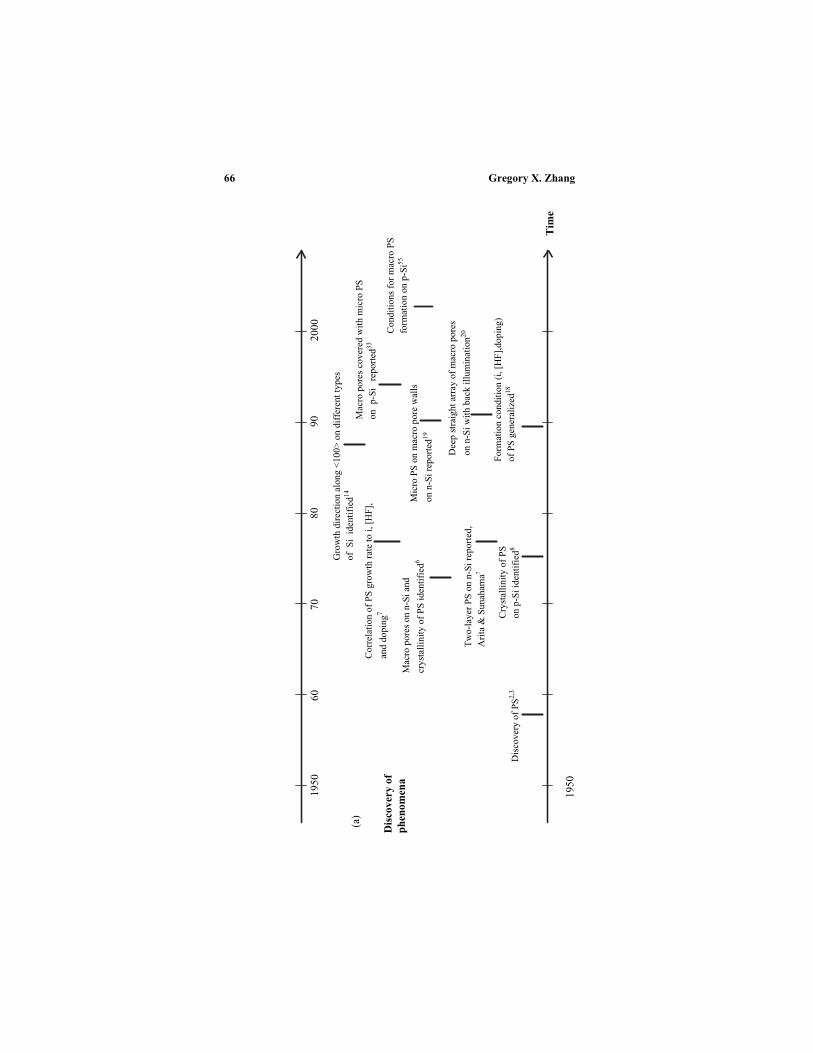
Gregory X. Zhang66
Cry
stal
lini
ty o
f P
S
on p
-Si i
dent
ifie
d8
Mac
ro p
ores
on
n-S
i and
crys
tall
init
y of
PS
iden
tifi
ed6
Dis
cove
ry o
f P
S2,
3
Tw
o-la
yer
PS
on
n-S
i rep
orte
d,A
rita
& S
unah
ama7
Cor
rela
tion
of
PS
gro
wth
rat
e to
i, [
HF
],
and
dopi
ng7
1950
1950
6070
8090
2000
For
mat
ion
cond
itio
n (i
, [H
F],
dopi
ng)
of P
S g
ener
aliz
ed18
Mic
ro P
S o
n m
acro
por
e w
alls
on n
-Si r
epor
ted19
Dee
p st
raig
ht a
rray
of
mac
ro p
ores
on n
-Si w
ith
back
illu
min
atio
n20
Mac
ro p
ores
cov
ered
wit
h m
icro
PS
on
p-S
ire
port
ed33
Gro
wth
dir
ecti
on a
long
<10
0> o
n di
ffer
ent t
ypes
of
Si
iden
tifi
ed14
(a)
Dis
cove
ry o
fph
enom
ena
Tim
e
Con
diti
ons
for
mac
ro P
Sfo
rmat
ion
on p
-Si55

nismsPorous Silicon: Morphology and Formation Mecha 67
1950
6070
8090
2000
PS
is d
isso
luti
on-
Pre
cipi
tati
on p
rodu
ct2
PS
on
n-S
i due
to lo
cal
brea
kdow
n of
dep
leti
on la
yer6
PS
for
mat
ion
due
todi
ffus
ion
of h
oles
14N
ano
pore
s on
p-S
idue
toqu
antu
m c
onfi
nem
ent22
PS
for
mat
ion
due
to s
ensi
tivi
ty o
f re
acti
ons
to s
urfa
ce c
urva
ture
24
PS
for
mat
ion
due
to e
nhan
ced
dis
solu
tion
by in
tens
ifie
d fi
eld
at p
ore
tip12
Mac
ro p
ores
on
p--S
idue
to h
ole
diff
usio
n in
spa
ce c
harg
e la
yer39
Por
es f
orm
due
to a
sil
icic
laye
r on
wal
ls9
Cur
rent
bur
st th
eory
40
Mac
ro p
ores
on
p-S
i con
trol
led
by r
esis
tivi
tyof
Si r
elat
ive
to e
lect
roly
te35
Tim
e
PS
as
a re
sult
of
a di
spro
port
iona
tion
rea
ctio
n4
(b)
Dev
elop
men
t of
theo
ries
Geo
met
ry -
rela
tivi
ty th
eory
1
1950
Figu
re 1
. P
rogr
ess
in t
he d
isco
very
of
mor
phol
ogic
al p
heno
men
a an
d in
the
dev
elop
men
t of
the
orie
s on
for
mat
ion
mec
hani
sms
ofpo
rous
sili
con.

Gregory X. Zhang68
brown film was a dissolution/precipitation product (Si0amorphous)resulted from a two-step disproportionation reaction.4
The formation of etch pits and tunnels on n-Si duringanodization in HF solutions was reported in the early 1970's. Itwas found that the solid surface layer is the remaining substratesilicon left after anodic dissolution. The large current observed onn-Si at an anodic potential was postulated to be due to barrierbreakdown.5,6 By early 80's7-11 it was established that the brownfilms formed by anodization on silicon substrate of all types are aporous material with the same single crystalline structure as thesubstrate.
Many theories on the formation mechanisms of PS emergedsince then. Beale et al.12 proposed that the material in the PS isdepleted of carriers and the presence of a depletion layer isresponsible for current localization at pore tips where the field isintensified. Smith et al.13-15 described the morphology of PS basedon the hypothesis that the rate of pore growth is limited bydiffusion of holes to the growing pore tip. Unagami16 postulatedthat the formation of PS is promoted by the deposition of apassive silicic acid on the pore walls resulting in the preferentialdissolution at the pore tips. Alternatively, Parkhutik et al.17
suggested that a passive film composed of silicon fluoride andsilicon oxide is between PS and silicon substrate and that theformation of PS is similar to that of porous alumina.
The conditions for formation of PS on all types of substratesin terms of current density and HF concentrations wereestablished by Zhang et al.18 by the end of 1980's. Whetherformation of PS occurs during anodization was found to belargely independent of the electronic properties of silicon such asdoping type and concentration, but depend on the nature ofelectrochemical reactions.
Lehmann and Foll9-11 in early 1990’s reported the formationof straight, smooth and well spaced macro pore arrays on n-Siusing backside illumination and surface patterning. Theypostulated that for these large straight pores the dissolution rate atpore tips are limited by mass transfer in the electrolyte and thatthe relative rates of carrier transport in the silicon semiconductorand mass transport in the electrolyte determine PS morphology.For the micro pores formed on p-Si, Lehmann and Gosele22-23
proposed a quantum confinement model; due to the quantum
nisms 69
confinement the pore walls are depleted of carriers and thus donot dissolve during the anodization. At about the same time,Zhang24 proposed the surface curvature model, which postulatedthat not only the rate but also the distribution of reactions on acurved pore bottom can be greatly affected by surface curvature.
In the late 1990’s, Foll et al.40-43 proposed the current bursttheory. The basic hypothesis is that the electrochemical reactionsinvolved in the dissolution of the silicon surface operate inmicroscopic units. These reaction units have a temporal and aspatial distribution in number and in the state of activity. Theformation of pores is due to the synchronization of these operationunits at certain time and geometrical scales.
Two-layer PS with a micro PS on surface of a macro PSformed on n-Si under front illumination had been reported in thelate 70's but was little investigated until the 90's.26-29 The microPS may have a fractal-like geometry; the structure can vary in thesame layer from amorphous to single crystalline and diameterfrom a few nm to hundreds of nm. It appeared that while theformation of a macro PS layer under front illumination followsthe same mechanism as the macro PS formed in the dark, theformation of micro PS is due to the effect of the photo generatedcarriers. According to Arita30 the drift current due to the photocarriers generated in the depletion layer is responsible for theamorphous-like PS. Alternatively, Clement et al.31 suggested thatthe micro PS formed under illumination could result fromshattering of the macro PS into fine filaments due to residualstress.
Formation of macro PS and two-layer PS on lowly doped p-Si in anhydrous organic HF solutions was first reported by Propstand Kohl32,33 in the mid 1990's. It was thought to be related to thechemistry of the organic solvents. Macro pores on lowly doped p-Si were later found to also form in aqueous solutions. Walls of themacro pores are not always covered by a micro PS layer.34-36
Wehrspohn et al.37,38 suggested that a necessary condition for theformation of macro PS on lowly doped p-Si is a higher resistivityof the substrate than that of electrolyte. This idea was sooninvalidated as macro PS was also found to occur in electrolysesthat have much higher resistance than the silicon substrate.34,39
Alternatively, Lehmann and Ronnebeck39 postulated that theformation of macro PS on lowly doped p-Si is due to the
Porous Silicon: Morphology and Formation Mecha
Gregory X. Zhang70
dominant effect of thermionic emission which is sensitive tobarrier height rather than barrier width. More recently, Zhang1
proposed that the formation of macro PS on lowly doped p-Si isdue to the non-linear potential distribution in the highly resistivesubstrate caused by surface curvature.
Some ideas have been elaborated with extensivemathematical formulation. For example, a theoretical modelingbased on charge transfer kinetics for PS morphology wasattempted by Jaguiro et al.44 Similar mathematical modelingconsidering the transport phenomena of carriers in thesemiconductor, ions in the electrolyte and surface tension wasproposed by Valance.45 An analytical formulation basedprincipally on thermodynamical arguments was offered byMonica et al.46
Most theories have dealt only with certain aspects of the verycomplex morphology and formation of PS. No single theory is yetclose to a globally coherent description of the extremely rich andcomplex nature of the reactions and the resulting morphologicalevolution of the silicon electrode surface involved in theformation of PS.1 Also, these theories on PS did not take intoaccount for the many details of anodic electrochemical reactionsand processes of the silicon electrolyte interface, which had beenextensively investigated. However, a complete description of thediverse morphological features of porous silicon requires theintegration of the all the morphological aspects as well as thefundamental electrochemical reaction processes involved insilicon/electrolyte interface. Any theory for the mechanisms ofporous silicon formation without such a global integration will belimited in the scope of its validity and the power to explainmorphological details. In addition, a globally and microscopicallyaccurate model also requires the full characterization of all themorphological features of PS.
A detailed and comprehensive review on all aspects of thefundamental and applied electrochemistry of silicon/electrolyteinterface was provided in a recently published book.1 Theobjective of this paper is to provide a conceptual analysis of themechanisms for the morphology and formation of porous siliconusing the large body of the information assembled in the book andto provide an integrated view of the formation mechanisms thatcan be coherent with the various morphological features on the
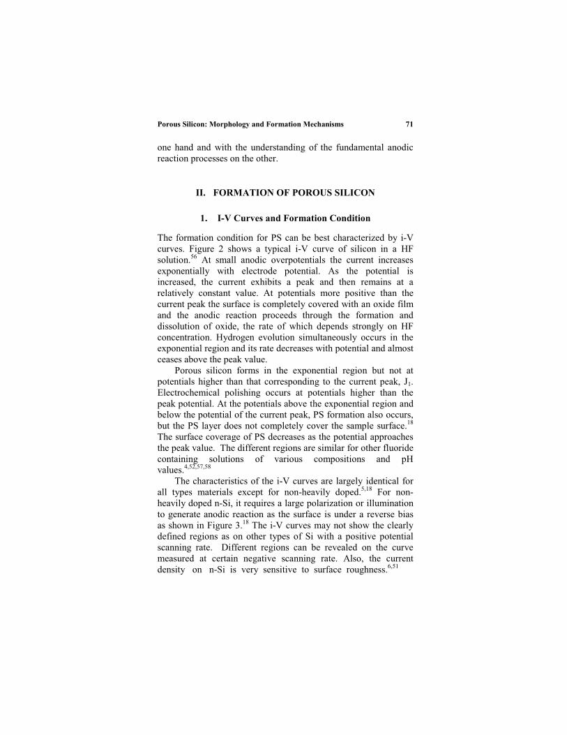
71
one hand and with the understanding of the fundamental anodicreaction processes on the other.
. FORMATION OF POROUS SILICON
1. I-V Curves and Formation Condition
The formation condition for PS can be best characterized by i-Vcurves. Figure 2 shows a typical i-V curve of silicon in a HFsolution.56 At small anodic overpotentials the current increasesexponentially with electrode potential. As the potential isincreased, the current exhibits a peak and then remains at arelatively constant value. At potentials more positive than thecurrent peak the surface is completely covered with an oxide filmand the anodic reaction proceeds through the formation anddissolution of oxide, the rate of which depends strongly on HFconcentration. Hydrogen evolution simultaneously occurs in theexponential region and its rate decreases with potential and almostceases above the peak value.
Porous silicon forms in the exponential region but not atpotentials higher than that corresponding to the current peak, J1.Electrochemical polishing occurs at potentials higher than thepeak potential. At the potentials above the exponential region andbelow the potential of the current peak, PS formation also occurs,but the PS layer does not completely cover the sample surface.18
The surface coverage of PS decreases as the potential approachesthe peak value. The different regions are similar for other fluoridecontaining solutions of various compositions and pHvalues.4,52,57,58
The characteristics of the i-V curves are largely identical forall types materials except for non-heavily doped.5,18 For non-heavily doped n-Si, it requires a large polarization or illuminationto generate anodic reaction as the surface is under a reverse biasas shown in Figure 3.18 The i-V curves may not show the clearlydefined regions as on other types of Si with a positive potentialscanning rate. Different regions can be revealed on the curvemeasured at certain negative scanning rate. Also, the currentdensity on n-Si is very sensitive to surface roughness.6,51
nismsPorous Silicon: Morphology and Formation Mecha
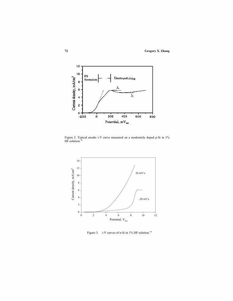
Gregory X. Zhang72
Figure 2. Typical anodic i-V curve measured on a moderately doped p-Si in 1%HF solution.18
Figure 3. i-V curves of n-Si in 1% HF solution.18
Potential, Vsce
10 12
Cur
rent
den
sity
, mA
/cm
2
0
2
4
6
8
10
12
14
Potential, Vsce
100 2 4 6 8 12
Cur
rent
den
sity
, mA
/cm
2
20 mV/s
-20 mV/s
0
2
4
6
8
10
12
14
73
Mechanical roughening can greatly increase the current density ata given potential. Current can arise on a rough surface at apotential several volts lower than that on a smooth surface.
Anodic dissolution of n-Si can also proceed at a polarizationunder illumination. The maximum current is limited byillumination intensity when the saturation photo current density islower than the critical current, J1. The characteristics of i-V curvesof n-Si under a high illumination intensity, when the reaction is nolonger limited by the availability of photo generated carriers, isidentical to that for p-Si. Similar also to p-Si, formation of PS onn-Si occurs only below the critical current, J1.
24
The dependence of i-V characteristics on doping is anindication of the carrier conduction mechanisms that can occur ina silicon substrate. When carrier supply in the silicon substrate isnot rate limiting, i-V curves obtained in different HFconcentrations are identical in characteristics.56 When the supplyof carriers in the substrate is rate limiting as determined by thedoping and illumination condition, i-V curves display distinctdifference between p-Si and n-Si, and for n-Si betweenilluminated and non-illuminated materials. For non-heavily dopedp-Si, the process is by thermal emission of holes while it is byZener tunnelling for heavily doped materials.10,59 For moderatelydoped n-Si the reaction is limited by the minority holes;significant current occurs when a large amount of holes aregenerated by illumination or when relatively high anodicpotentials are applied to allow interface tunneling to occur.11,62
Examination of the sample surfaces that are anodized atdifferent potentials indicates that the potential corresponding tothe maximum slope of the i-V curve is the upper limit forformation of a porous silicon layer that covers uniformly theentire surface. At potentials between the maximum slope andcurrent peak, porous layer may still form but the surface coverageis not uniform. Plotting the current at the maximum slope and thepeak current for different types of silicon as a function of HFconcentration, the condition for occurrence of PS formation andelectropolishing is obtained as shown in Figure 4.18 This figurealso shows that the three regions in relation to current density andHF concentration are essentially independent of the siliconsubstrate doping type and concentration. This means that the
nismsPorous Silicon: Morphology and Formation Mecha

Gregory X. Zhang74
Figure 4. Formation condition for porous silicon; solid line - peak currentdensity, dotted line - current density at the maximum slope (see Figure.2).18
differences in semiconducting properties of the silicon sampleshave little effect on the occurrence of these regions. The variousparameters involved in PS formation such as potential, doping,and illumination, affect the occurrence of different regionsthrough their relation to the current density. Low current densityand high HF concentration favour PS formation while highcurrent and low HF concentration favours polishing.
Electropolishing region does not occur in anhydrous organicsolutions due to the lack of water which is required for theformation of oxide film. Figure 5, as an example, shows that inanhydrous HF-MeCN solution the current can increase withpotential to a value of about 0.5 A/cm2 without showing a peakcurrent. The relationship between current and potential is lineardue to the rate limiting effect of resistance in solution and siliconsubstrate.

5
Figure 5. i-V behavior of p-Si in 2M HF + 0.25M TBAP in MeCN and in 2MHF + 1M NH4F in H2O, After Propst and Kohl.33
2. Hydrogen Evolution and Effective Dissolution Valence
Evolution of hydrogen gas occurs during the formation of PS inaqueous solutions. The amount of hydrogen gas is proportional tothe time of anodization.4 Due to hydrogen evolution, which is achemical reaction, the effective dissolution valence of silicon, n,can vary between 2 to 4 depending on the relative contribution ofthis reaction. In general, n increases with increasing anodiccurrent density as the amount of hydrogen evolution reduces; thechange is sharpest near the peak current density J1. At a givencurrent density, n increases with HF concentration. Also,dissolution valence decreases with increasing PS layer thickness.Dissolution valence as low as 0.5 can be measured for thick PSfilms formed at low current densities. The low n values are due tochemical dissolution of PS during the time of its growth. Thethicker the PS layer the longer the sample is in the electrolyte andthe larger the amount of chemical dissolution. This effect isparticularly significant for the PS formed on p-Si, which hasextremely fine pore structure and thus large surface area.
Porous Silicon: Morphology and Formation Mechanisms 7
Potential, Vsce
-2 -1 0 1 2 3
Cur
rent
den
sity
, A/c
m2
-0.1
0.0
0.1
0.2
0.3
0.4
0.5
P-Si, 13Ωcm
HF in MeCN
HF in H2O

Gregory X. Zhang76
The formation of hydrogen does not occur in anhydrousorganic solvents.32,33,63 Due to the lack of hydrogen evolution,dissolution valence is near 4 at all current densities. Addition ofwater in the organic solvents reduces the dissolution valence.
3. Growth Rate of Porous Silicon
The growth rate of a PS layer can vary over a wide rangedepending on formation conditions. It can be as low as a few Å/sand as high as 4000 Å/s.7,17 For p-Si the growth rate of PS at agiven current density appears to increase linearly with respect toHF concentration and current density.7,64 For n-Si the growth rateincreases also with HF concentration and current density but therelations are not linear (Figure 6).7,19,65 Also, for p-Si, it increaseslinearly with logarithmic dopant concentration but for n-Si thedependence of growth rate on dopand concentration is morecomplicated. Temperature of HF solutions generally has little
Figure 6. Effect of current density on PS formation rate, after Arita andSunahama.7
Current density, mA/cm2
0 20 40 60 80 100 120
Gro
wth
rat
e, A
/s
0
500
1000
1500
2000
52mW/cm2
22 mW/cm2
0.006 Ωcm
1.6 Ωcmp-Si(111)
n-Si(111)2.5Ωcm

77
influence on growth rate of PS.2,66 PS growth rate is generallyhigher on (100) substrates than on (111) substrates.67
Figure 7 shows that PS thickness increases linearly with timeup to certain thickness.16,17 Such constant growth rate at a constantcurrent density means that the PS formed is uniform in thickness(Effective surface area remains constant assuming reactionkinetics is the same). At a large thickness the growth may deviatefrom linearity due to the effect of diffusion in the electrolytewithin the pores.19,25 It has been found that for a very thick PSlayer (150 µm) there is about 20% difference in HF concentrationbetween that at the tips of pores and that in the bulk solution.19
Figure 7. Kinetic dependance of the PS thickness on anodization time, afterParkhutik et. al.17
nismsPorous Silicon: Morphology and Formation Mecha
Time, min0 10 20 3 0
Thi
ckne
ss,µ
m
0
2
4
6
8
10
12
14n-Si(111), 0.01Ωcm48% HF
0.1 mA/cm2
1
530
Time, min
0 10 20 30 40
Thi
ckne
ss,µ
m
0
2
4
6
8
10
12
14n-Si(111), 0.01Ωcm48% HF
0.1 mA/cm2
1
530
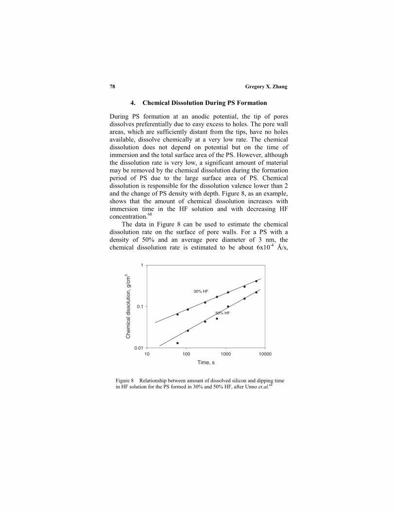
Gregory X. Zhang78
4. Chemical Dissolution During PS Formation
During PS formation at an anodic potential, the tip of poresdissolves preferentially due to easy excess to holes. The pore wallareas, which are sufficiently distant from the tips, have no holesavailable, dissolve chemically at a very low rate. The chemicaldissolution does not depend on potential but on the time ofimmersion and the total surface area of the PS. However, althoughthe dissolution rate is very low, a significant amount of materialmay be removed by the chemical dissolution during the formationperiod of PS due to the large surface area of PS. Chemicaldissolution is responsible for the dissolution valence lower than 2and the change of PS density with depth. Figure 8, as an example,shows that the amount of chemical dissolution increases withimmersion time in the HF solution and with decreasing HFconcentration.68
The data in Figure 8 can be used to estimate the chemicaldissolution rate on the surface of pore walls. For a PS with adensity of 50% and an average pore diameter of 3 nm, thechemical dissolution rate is estimated to be about 6x10⁻⁴ Å/s,
Figure 8 Relationship between amount of dissolved silicon and dipping timein HF solution for the PS formed in 30% and 50% HF, after Unno et.al.68
Time, s
10 100 1000 10000
Che
mic
al d
isso
lutio
n, g
/cm
3
0.01
0.1
1
30% HF
50% HF
79
assuming the PS consists of straight cylindrical pores of an equaldiameter. The order of magnitude is in agreement with the planaretch rate of silicon in concentrated HF solutions.
. MORPHOLOGY OF PS
Morphology, which is determined by the distribution of materialsin space, is the least quantifiable aspect of a material. It is thusvery difficult to characterize morphology of PS, which hasextremely rich details with respect to the range of variations inpore size, shape, orientation, branch, interconnection, anddistribution. Qualitatively, the diverse morphological features ofPS reported in the literature can be summarized by Figure 9 withrespect to four major different aspects: pore orientation, fill ofmacro pores, branching, and depth variation of a PS layer.
1. Pore Diameter
Among the morphological features, the average pore diameter of aPS, as a quantifiable and easily measurable parameter, is mostcommonly determined. Table 1 shows some examples for porediameter and interpore spacing reported for the PS formed undervarious conditions. The pores are categorized in this followingtext as micro pores (less than 10 nm) and macro pores (larger than50nm). Pores with size between 10 and 50 nm are grouped intoeither micro or macro pores depending on the specific situation.
(i) Effect of Doping
The diameter of pores and interpore spacing may vary withdoping type and concentration in a wide range, from about 1 nmto about 10 µm, about 4 orders of magnitude.14,73,80,81 The PSformed on different substrates can be roughly grouped into fourmain categories according to doping concentration: 1. moderatelydoped p-Si (1015-1018); 2. heavily doped materials, p+-Si and n+-Si(> 1019); 3. non- heavily doped n-Si (< 1018); and 4. lowly dopedp-Si (< 1015). The PS formed on moderately doped p-Si hasextremely small pores ranging typically from 1 to 10 nm. Forheavily doped p and n types, the pores have diameters
nismsPorous Silicon: Morphology and Formation Mecha

Gregory X. Zhang80
(a)
(b)
(c)
(d)
(e)
(f)
(a)
(b)
(c)
(d)
(100
)(1
11)
(111
)(1
11)
(1)
Ori
enta
tion
(a)
ali
gned
to <
100>
an
d so
urce
of
hole
s
(b)
rou
ghly
ali
gned
to
sou
rce
of h
oles
(c)
par
tial
ly a
lign
ed to
<10
0>
and
sour
ce o
f ho
les
(d)
ali
gned
onl
y to
<10
0>
(2)
Bra
nchi
ng(a
) s
moo
th p
ore
wal
l(b
) b
ranc
hes
shor
ter
than
dia
met
er(c
) s
econ
d le
vel b
ranc
hes
only
(d)
den
drit
ic b
ranc
hes
(e)
mai
n po
res
wit
h se
cond
an
d th
ird
leve
l bra
nche
s
(f)
den
se, r
ando
m a
nd s
hort
bra
nche
s

nismsPorous Silicon: Morphology and Formation Mecha 81
(a)
(b)
(c)
(a)
(b)
(c)
(3)
Fill
of
mac
ro p
ores
(a)
unf
ille
d w
ith
mic
ro P
S
(b)
par
tial
ly f
ille
d
(c)
ful
ly f
ille
d
(4)
Dep
th v
aria
tion
of
PS
laye
r
(a)
sin
gle
laye
r of
mic
ro P
S
(b)
sin
gle
laye
r of
mac
ro P
S w
ith
smal
ler
pore
s ne
ar th
e su
rfac
e
(c)
a la
yer
of m
icro
PS
on
top
of m
acro
PS
(P
ores
may
be
fill
e
by m
icro
PS
)
Figu
re 9
. M
orph
olog
ical
cha
ract
eris
tics
of
poro
us s
ilico
n .

Gregory X. Zhang82
Table 1
Examples of Pore Diameter, Interpore Spacing and Pore
Density of the PS Formed under Different Conditions (a More
Extensive List is Given in Ref.1)
Material.cm
Solution% HF
CurrentmA/cm2
Diameterµm
Spacingµm
Ref.
p(100)
0.001 20 100 0.05 0.01 59 0.006 33 50 0.005 69 0.006 24 + 47% eth 200 0.002 0.0015 70 0.01 10 10 0.0052 60 0.01 69 30 0.006 0.015 71 0.02 25 + 50% eth 30 0.05 0.02 72 1 49 30 0.003 71 13 2 M HF + MeCN 7 1–2 2–3 33 20 3 2 1.5–3, MPc 1–3 39 25 48 10 0.0025 12 50 10 3 2.4–4, MP 1–2 39100 25 20 3–6, MP 0.5 73224 2 M HF + MeCNb 7 1–2 0.5–2 32
(111) 10 50 20 0.004 74 10 50:etha.(1:3) 20 0.004 74
(110) 0.01 49 2 0.005 14 0.4 24 + 47% eth 50 0.035 0.01 70
n-Si(100)
0.002 1 4 0.05 0.05 650.007 15 65 0.004 60
0.01 5 0.1 V, 15 mA,illu.
1–4 0–4 27
0.03 4 4 0.05 0.3-0.8 750.1 49 80 0.06 760.1 5 6 V 0.14 0.44 240.1 20 50 0.009 0.03 770.1 20:60, HF:eth 50 mA 0.08 0.1 59
1 2.5 0.5, 10 V,illu., B
0.6 6.9 20
3 10:35, HF:eth 1.2 V, 5mAillu.
0.33 1–2 78
5 6 3 V, 10 mAillu.Ba
2.5 5 19
10 20:60, HF:eth 50 mA 0.8 > 0.5 5920 2.5 1.5, 10 V,
illu., B2 5.5 20
83
Table 1
ContinuationMaterial
.cmSolution
% HFCurrentmA/cm2
Diameterµm
Spacingµm
Ref.
(111)0.01 12–48 20 0.01 790.008 25:50, HF:eth 50 0.01 0.03 802.5 50 30, 7 mW 1.5 72.5 50 90, 54 mW 1.7 30
(110)0.82 49 80 0.01 0.1 133 4 4, 1.5 V 2–4 1–2 39
a B: backside illuminationb MeCN: acetonitrilec MP: macropores of two-layer PSd eth: ethanol,
typically ranging from 10 to 100 nm. For non-heavily doped n-Si,the pores have a wide range of possible diameters from 10 nm to10 µm. For lowly doped p-Si, the PS can have two distinctdistributions of pore diameters: large pores with a distribution ofdiameters in the order of µm and small pores on the order of nm.The effect of doping on pore diameter strongly depends onsolution composition, potential and illumination conditions.
Figure 10 shows that for n-Si the diameter of the poresdecreases with doping concentration at different currentdensities.80 In contrast, the pore diameter of p-Si of moderate orhigh doping concentrations decreases with increasing dopingconcentration. In the transition region (Figure 4), macro pores canform on all types of substrates, in which the silicon surface ispartially covered with an oxide film, and the morphology of PStype strongly depends on solution composition.18,27,73,75,82,83 Themacro pores formed on p-Si in the transition region have beeninvestigated in a recent study in various solutions.55
(ii) Effect of Potential, Current and HF Concentration
Pore diameter generally increases with increasing potentialand current density.9,24,60,80 Figure 10 shows that the diameter ofpores formed on both p-Si and n-Si increases with current
nismsPorous Silicon: Morphology and Formation Mecha
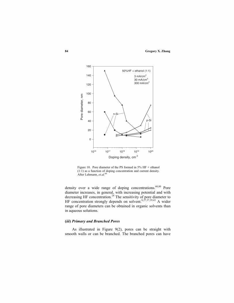
Gregory X. Zhang84
Figure 10. Pore diameter of the PS formed in 5% HF + ethanol(1:1) as a function of doping concentration and current density.After Lehmann, et.al.80
density over a wide range of doping concentrations.60,80 Porediameter increases, in general, with increasing potential and withdecreasing HF concentration.24 The sensitivity of pore diameter toHF concentration strongly depends on solvent.8,27,37,39,43 A widerrange of pore diameters can be obtained in organic solvents thanin aqueous solutions.
(iii) Primary and Branched Pores
As illustrated in Figure 9(2), pores can be straight withsmooth walls or can be branched. The branched pores can have
Doping density, cm-3
1016 1017 1018 1019 1020
Por
e di
amet
er, n
m
0
20
40
60
80
100
120
140
160
50%HF + ethanol (1:1)
3 mA/cm2
30 mA/cm2
300 mA/cm2
n-Si
p-Si

85
third level or further levels of branches. Branched and hierarchicalpore structure has been found to form on all types of substrates.Branched pores are generally smaller than the primarypores.12,14,76,84
(iv) Surface-Patterned PoreAarrays
Straight large pores with smooth walls can be formed bybackside illumination of n-Si of (100) orientation.19,20,85 Usingmicro patterning for pore initiation sites on the surface regularlyspaced pore arrays can be produced. Production of pore arrays of2 µm in diameter up to 400 µm deep on 6 in wafer have beenreported.86 Well aligned pore arrays have not been obtained on(111) and (110) wafers due to the misalignment between thedirection of pore growth and that of the hole source.87
Under a given formation condition, the pores beyond thesurface region have certain size determined by the formationconditions (i.e., HF concentration, current density, potential anddoping concentration). According to Lehmann et al.,87 thesmallest possible pore diameter for a regular pore array formedwith surface patterning and backside illumination is about 0.3µmbelow which branching at pore bottom occurs; the largest poresare found to be about 20 µm, above which formation of straightand smooth pores becomes a problem due to hydrogen bubbleformation.
(v) Variation From Surface To Bulk
The pores at the surface are smaller than those in the bulk of PSas, for example, shown in Figure 11.8,16,24 Such an increase inpore diameter from the surface to bulk is due to the transitionfrom pore initiation to steady growth. Also, two-layer PS, a microPS layer on top of a macro PS can form for on illuminated n-Si oron lowly doped p-Si.19,26,78 For the micro PS layer formed on frontilluminated n-Si, pore diameter is less than 2 nm and thickness ofPS changes with illumination intensity and the amount of chargepassed. Also, the diameter of macro pores on front illuminated n-Si changes with the amount of charge Passed.20 Pore size anddepth variation of PS on n-Si are very different for front and backilluminated n-Si samples.
nismsPorous Silicon: Morphology and Formation Mecha

Gregory X. Zhang86
Figure 11. SEM photograph showing smaller pore diameter and larger poredensity near the surface than in the bulk in 5% HF at 6 V.24
For very deep pores the diameter may increase with adecreased growth rate due to the effect of diffusion process insidepores. The depth at which this occurs depends on current densityand HF concentration.87 Low HF concentration, low temperatureand low growth rate favour formation of deep uniform pores.
(vi) Interpore Spacing
The variation of interpore spacing or wall thickness is morecomplex than pore diameter. There is not much information on therelationship between wall thickness and formation conditions. Ingeneral, the walls are on the same order as or smaller than porediameter.24 In particular, interpore spacing depends on potential; itincreases with potential at small currents but at certain current itstarts to decrease with increasing potential. When interporespacing is reduced to zero, which occurs in the transition region,pores no longer form, and instead, shallow pits form.

87
(vii) Distribution of Pore Diameter
Pore diameters of the PS layer formed under a given set ofconditions have a distinct distribution. Normal, log-normal,bimodal, fractal, and non-uniform distributions have been foundfor PS formed under different conditions.26,29,60,88,89,90,91
For the PS formed on heavily doped silicon, pore diameterhas a narrower distribution at a lower current at a given HFconcentration and the distribution is narrower at a lower HFconcentration at a given current desnity. Bimodal distribution ofpore diameter are generally associated with two layer PS on lowlydoped p-Si and illuminated n-Si. Pores with multiple distributionshave been observed for the PS that has a surface micro pore layerand smaller branched pores in addition to the main pores.88,90
Distribution of pore diameters for highly branched PS has beenfound to be fractal-like.14,76 Illumination during formation of PSon p-Si can also to affect the distribution of pore diameter; itincreases the amount of the smaller nanoscrystals, while reducesthe amount of larger crystals.92 For the PS formed under anilluminated substrate, the relative amount of small crystals tendsto increase with reduction of light wavelength.93
2. Pore Orientation and Shape
The growth of individual pores, or the dissolution at pore tips, isanisotropic, depending on the orientation of the substrate and thedirection of the carrier source. The relative effect of substrateorientation and direction of the carrier source on the orientation ofpores is determined by the specific electrochemical reactions atthe pore bottoms.
The orientation of primary pores is in general in the <100>direction for all the PS formed on all types of (100)substrates.7,14,84 For the PS with dendritic structure, as shown inFigure 12, pores propagate along (100) direction even on the(110) and (111) substrates.20,84,94 The branched pores of non-dendritic types formed on (100) substrate may not be strictlyperpendicular to the primary pores but deviate to various extentsfrom the <100> direction toward to the source of holes.12,14,95
Ronnebeck et al.95 found that the macro pores formed on
nismsPorous Silicon: Morphology and Formation Mecha

Gregory X. Zhang88
Figure 12. Dendritic PS morphology formed on n (100),12 cm in 4% HF at 4 mA/cm2. After Jäger, et. al.84
Figure 13. Preferential growth of pore on 35oC from
(100) n-Si with back illumination. After Ronnebeck et.
al.95
89
misoriented n(100) substrates (from 150 to 350) as well as onn(111) are oriented along <100> direction when they are formedin the dark at high anodic potentials. However, when the samplesare illuminated from the back, the pores formed on the (111)sample and the side pores formed on the 350 misoriented (100)sample are oriented along <113> as shown in Figure 13.
For pores of extremely small diameters, in the order of a fewnm, the direction of individual pores is totally random. On theother hand, large pores tend to have less anisotropic effect andgrow more dominantly in the direction of carrier supply, that is,perpendicular to the surface. The macro pores formed on p-Sigenerally have smooth walls and an orientation toward the sourceof holes that is perpendicular to the surface, even on (110) and(111) samples.34,39
Depending on substrate orientation and formation condition,individual pores may have different shapes. The shape of thepores formed on (100) substrate is a square bounded by 011planes with corners pointing to the <100> directions.14,77 Theshape of individual pores formed on n-Si tends to change fromcircular to square to star-like and to dendrite-like with increasingpotential.20 Low formation voltage tends to favour circular shapewhile high voltage favours star-like shape. Near perfect squareshape of pores can be obtained for the PS formed on n-Si undercertain conditions.
The bottom of individual pores is always curved, varyingfrom a shallowly curved semicircle to an elongated conicaldepending on the formation conditions. As will be discussed laterthe curvature of pore bottom plays a critical role in the reactionkinetics required for formation of PS and its morphology.
3. Pore Branching
Individual pores, depending on formation conditions, maypropagate straight in the preferred direction with very littlebranching or with formation of numerous side or branched pores.In general, the conditions that favour the formation of small poresalso favours branching.
The degree of branching and interpore connection dependsstrongly on doping concentration. The most highly connected PS
nismsPorous Silicon: Morphology and Formation Mecha

Gregory X. Zhang90
Figure 14. Straight pores with smooth wall formedon n-Si in the dark.1
is found in the PS of lowly doped p-Si and the micro PS onilluminated n-Si.14 On the other hand, well separated and straightpores are generally found on moderately or lowly doped n-Si.Perfectly straight pores with smooth walls can be formed on n-Siin the dark, as for example, shown in Figure 14.65 Also, on n-Sismooth and straight pores without branching can be obtainedunder back illumination using surface patterned substrate. Forheavily doped materials, pores are generally branched.12,71 Fornon-heavily doped p-Si, pores are highly branched resulting in arandom network of pores. The macro pores formed on lowlydoped p-Si generally have no side pores longer than the porediameter.32,34,39
Like main pores, branched pores are highly directional,propagating preferentially in the 100 planes and the long <100>directions.14,20,77 Such directional branching can produce regularlyspaced three dimensional structures as shown in Figure 15.14,65
The tendency to branch is stronger on (110) and (111) substratesthan on (100) because for substrates of non-(100) orientations,<100> direction does not coincide with the direction of the holesource. Due to the large tendency to branch, it is difficult to

91
Figure 15. Three dimensioned structures generated bythe formation of dendritic pores on an n(110)substrate.1,14
produce straight perpendicular pores with smooth walls on(110) and (111) samples, even on surface patterned samples.87
4. Interface Between PS and Silicon
The growth of a PS layer (not individual pores) is alwaysperpendicular to the surface of the substrate with back electricalcontact. The growth front is planar, independent of the orientationof the silicon samples. The interface between PS layer and silicon
nismsPorous Silicon: Morphology and Formation Mecha
(a)
(b)

Gregory X. Zhang92
substrate is essentially flat with high and low points deferringwithin a few microns.
5. Depth Variation
The morphology of PS generally varies in the depth directionfrom the surface to the bulk. There are two types of depthvariations: 1) the change of pore diameter is gradual from thesurface to the bulk where pore diameter is constant; and 2) thechange of pore diameter is abrupt from a surface layer to the bulklayer with a difference in diameter as large as three orders ofmagnitude. The surface layer for the first type is a transition layerformed due to the transition from initiation of pores to the steadystate growth. The second type is two-layer PS with a micro PS ontop of a macro PS. While two-layer PS forms only under certainconditions, the transition PS layer of varying thickness exists onthe surface of all PS layers.
(i) Transition Layer
Transition layer is found to exist for all types ofsilicon.7,16,20,24,25,80 The pores in the transition layer are generallymuch smaller than those in the bulk. There is not a clearlydefinable boundary that separates the surface layer and the bulk.The thickness of the transition layer is related to the size of pores;the smaller the pores the thinner the surface transition layer. Forn-Si, the transition layer can be clearly seen as for example shownin Figures 11 and 16.24 On the other hand, for p-Si this surfacelayer is very thin (near zero) for some PS with extremely smallpores. Such thin layer may not be observed because it may beremoved due to chemical dissolution during its exposure insolution.
The morphology of the transition layer, unlike the bulkmorphology, depends sensitively on surface conditions,particularly surface roughness such as scratches.14,94 For n-Si,which usually requires a large potential to generate current in thedark, formation of PS can occur at much lower potentials if thesurface is roughened mechanically.
A certain amount of uniform dissolution may occur prior toand during the initiation of pores. Such an etched layer prior to the

93
Figure 16. Variation of diameter of pores from the surface tothe bulk. After Zhang.24
initiation of pores is involved in all types of PS since the etching,which causes roughening of the surface, is required for poreinitiation.84,95 The thickness of etched layer is generally in theorder of pore diameter.
(ii) Two-Layer PS
Two-layer PS, with a micro PS layer on top of a macro PSlayer, forms only under certain conditions. For n-Si, formation oftwo-layer PS is associated with front illumination, although it canalso be formed with back illumination.19,27,34,37 For p-Si, two-layerPS are found to form on lowly doped substrates. For moderatelyor highly doped p-Si or for n-Si in the dark, formation of two-layer PS has not been observed.
Formation of two-layer PS on front illuminated n-Si dependson the wavelength of light; formation of large and deep pores doesnot occur with a white light at wavelength < 800 nm, but occurs atwavelength > 867 nm.20 This phenomenon is due to thewavelength dependent absorption depth; carriers which aregenerated deep in the bulk promote pore growth at the tips ofmacro pores whereas those generated near surface result in theformation and dissolution of micro PS and lateral growth of themacro pores.
nismsPorous Silicon: Morphology and Formation Mecha
400 nm

Gregory X. Zhang94
There is a correlation between the occurrence of two-layer PSand the saturation photo current value.78 Only a single micro PSlayer forms at a photo current density below the photo saturationvalue while two-layer PS forms at current densities above thesaturation current as shown in Figure 17. Also, macro PS layerforms only after a certain amount of charge determined by theamount of etch required for the initiation of macro pores.77
There is also an etched layer of Si on the surface underillumination as illustrated in Figure 18. This etched layer ismainly due to photo-induced corrosion. As a result of the photoinduced dissolution the top surface of PS layer recedes with time.The rate of dissolution depends on doping, HF concentration,current density and illumination intensity.
Figure 17. Voltammograms of n-Si electrodes in aqueous solution containing10 wt.% HF and 35 wt.% C2H5OH at 5 mV s-1 under different light intensities.The illumination intensity was adjusted by changing the distance between the lightsource and the n-Si electrode. After Osaka et.al,78
Potential, Vsce
-0.5 0.0 0.5 1.0 1.5
Cur
rent
den
sity
, mA
/cm
2
0
5
10
15
20
0.7 mW/cm2
3 mW/cm2
12 mW/cm2
One layer
Micro PS
Two layer PS
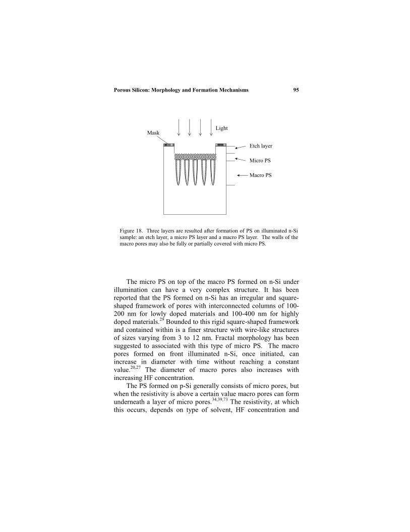
95
Figure 18. Three layers are resulted after formation of PS on illuminated n-Sisample: an etch layer, a micro PS layer and a macro PS layer. The walls of themacro pores may also be fully or partially covered with micro PS.
The micro PS on top of the macro PS formed on n-Si underillumination can have a very complex structure. It has beenreported that the PS formed on n-Si has an irregular and square-shaped framework of pores with interconnected columns of 100-200 nm for lowly doped materials and 100-400 nm for highlydoped materials.29 Bounded to this rigid square-shaped frameworkand contained within is a finer structure with wire-like structuresof sizes varying from 3 to 12 nm. Fractal morphology has beensuggested to associated with this type of micro PS. The macropores formed on front illuminated n-Si, once initiated, canincrease in diameter with time without reaching a constantvalue.20,27 The diameter of macro pores also increases withincreasing HF concentration.
The PS formed on p-Si generally consists of micro pores, butwhen the resistivity is above a certain value macro pores can formunderneath a layer of micro pores.34,39,73 The resistivity, at whichthis occurs, depends on type of solvent, HF concentration and
nismsPorous Silicon: Morphology and Formation Mecha
Etch layer
Micro PS
Macro PS
MaskLight
Gregory X. Zhang96
current density. In aqueous HF solutions macro pores are found toform on substrates of resistivity higher than 5 cm.39 On the otherhand, macro pores has been found to form on substrate with aresistivity of 1 cm in 2M HF + dimethylformamide electrolyte.34
Presence of water in organic solvents tends to reduce thethickness of the micro PS layer.
(iii) Fill of Pores
The macro pores of two-layer PS may be completely filled oronly partially filled with micro pores depending on the solutioncomposition.39,63 When other conditions are the same, macropores formed in organic solvents tend to be more filled than thoseformed in aqueous solutions. Addition of water to organicsolutions reduces the extent of filling. Among organic solutions,according to Jager et al.,54 the degree of filling of the macro poresformed on p-Si depends on the oxidizing nature of the solutions:macro pores are filled with micro PS in non-oxidizing electrolytesuch as acetonitrile (MeCN), while they are not filled foroxidizing electrolytes such as dimethylformamide (DMF).
For the two-layer PS formed on front illuminated n-Si, thedegree of filling of the macro pores depends on light intensity, onthe amount of charge passed, as well as on the magnitude of thecurrent relative to the saturation photo current.26,27,29,78 Thethickness of micro PS increases with the amount of charge passedand it decreases with increasing light intensity.27 The macro poresformed on lowly doped n-Si under back illumination can also befilled by micro PS and the degree of filling decreases withincreasing potential.19
6. Summary
The morphology of PS has extremely rich details determined bythe numerous factors involved in the anodization. Generally, p-Siand n-Si have distinct differences in the correlation between PSmorphology and formation conditions. Among all formationconditions doping concentration appears to show the most clearfunctional effect on morphology. A summery of morphologyfeatures of PS is provided in Table 2.

97
Table 2
Morphological Characteristics of Porous Silicona
Size
1. A PS layer may have one or two distinct distributions of pores with sizesvarying from 1nm–10µm. Those less than 10 nm are micro pores and thoselarger than 50 nm are macro pores.
In the darkmoderately doped p-Si (1015–1018): one distribution, 1–10 nm.heavily doped p-Si and n-Si (> 1019): one distribution,10–100 nm.non-heavily doped n-Si (< 1018): one distribution,10 nm–10µm.lowly doped p-Si (< 1015): one or two distributions, 1–10 nm and > 1µm.
IlluminationLittle effect on p-Si.For n-Si, one or two distributions 1–10 nm and 50 nm–10 µm.
2. For p-Si pore diameter increases with doping concentration; for n-Si, itdecreases with doping concentration.
3. It increases with potential or current density but decreases with HFconcentration.
4. Branched pores are smaller than primary ones.5. It is constant in the bulk but is smaller near the surface.6. Inter-pore spacing can be smaller than pore diameter but is not larger than trice
the diameter. It varies with the factors similarly as pore diameter.
Orientation
1. Pores grow preferentially along <100> directions and toward the source ofholes.
2. Well aligned macro pores, > 50 nm are perpendicular to the surface for (100)substrate but may have a less than 900 angle to the surface on othersubstrates.
3. Pores can be fully aligned with <100> directions or/and with source of holes.Pores with smooth wall tend to be aligned with source of holes, whiledendritic pores are aligned with <100> directions.
4. Very small pores, < 10 nm, do not show clear orientations.
Branching
1. PS has discrete pores with no branches, with short branches, or with dendriticbranches, or have no primary but densely and randomly branched pores.
2. Tendency to branch increases with decreasing pore diameter.3. Direction of branching has the same tendencies as pore orientation.
Fill of pores
1. In PS of two distributions, macro pores may be partially or fully filled by micropores.
2. It tends to occur in organic solvents; addition of water reduces the extent offilling.
3. Extent of filling decreases with increasing light intensity or increasingpotential.
nismsPorous Silicon: Morphology and Formation Mecha

Gregory X. Zhang98
Table 2. Continuation
Depth variation
1. Two types: transitional layer, which has no clear boundary with bulk and twolayer type with clear boundary between micro and macro PS layers.
2. Transitional layer is associated with the initiation of pores with smaller pores atthe surface.
3. Two layered PS occurs only on illuminated n-Si and lowly doped p-Si.4. Pore diameter and distribution is uniform in the bulk of PS.
Others
1. The bottom of pores is curved with the smallest curvature at the tips.2. The shape of pores can be square, dendritic, circular, and star-like.3. Interface of PS/Si is flat and is perpendicular to the source of holes.4. PS with macro pores has the same composition and crystalline structure as the
substrate; PS with micro pores can be amorphous and highly hydrogenatedand/or oxidized.
5. Pore wall is rough at atomic scale for all pores.a Based on information summarized in Ref. 1.
IV. ANODIC REACTION KINETICS
1. Potential Distribution and Rate Limiting Process
There are five possible physical phases in the current path inwhich the current conduction mechanisms are different asillustrated in Figure 19. They are substrate, space charge layer,Helmholtz layer, surface oxide film, and electrolyte. The overallchange in the applied potential due to a change of current densityin the current path is the sum of the potential drops in thesephases:
Vapp = VSi + Vs + VH + Vox + Vel (1)
The distribution of the applied potential in these different phasesdepends on silicon material as well as potential range. Table 3 is asummary for the potential distribution of different materials in thethree potential regions (Figure 2). While the distribution of thepotential below the passivation potential Vp (potential at currentpeak J1 in Figure 2) depends on doping type and concentration,

99
r1 & r2 - majority & minority carrier transport,r3 - transport of holes to the surfacer4 - charge transfer across the Helmhotz layer,r5 - electron injectionr6 - chemical dissolution,r7 - oxide formation,r8 - ionic transport in oxide,r9 - injection of oxidants,r10 - dissolution of oxide,r11 - mass transport in electrolyte
Figure 19. Schematic illustration of the processes involving the transport ofcharge and species in the different phases in the interface region.
Table 3
Distribution of the Applied Potential in the Electric Layers at
the Silicon/Electrolyte Interface in HF Solutions
Material OCP to V (i ~ 0)a Exponential region V > Vp
Heavily doped p,n-Si
Helmholtz layer Helmholtz layer Oxide film
Non-heavily dopedn-Si
Space charge layer Space charge layer Oxide film
Non-heavily dopedp-Si
Space charge layer Helmholtz layer &space charge layer
Oxide film
aOCP, V (I ~ 0), Vp: defined in Figure 2.
nismsPorous Silicon: Morphology and Formation Mecha
Si Electrolyte
r8
r9
r6
r7
r4
r5r1
r2r10
r11
Helmholtz layerOxideSpace charge layer
r3
rr
Gregory X. Zhang100
the applied potential is principally dropped in the oxide film at apotential higher than Vp for all materials.
For n-Si the applied potential is predominantly droppedacross the space charge layer in the semiconductor. For p-Si andheavily doped n-Si, distribution of potential is partitioned betweenthe Helmholtz layer and/or the space charge layer.18,48-51 Forheavily doped materials the surface is degenerated and thematerial behaves like a metal electrode, meaning that the chargetransfer reaction in the Helmholtz double layer is the ratedetermining step and potential drops mostly in the Helmholtzlayer. For non-heavily doped p-Si, the potential is mostly droppedwithin the space charge layer before the onset of current. Atpotentials higher than that at which current becomes measurable,the change in potential may be dropped also in the Helmholtzlayer in addition to the space charge layer. Also, for very lightlydoped material, potential drop in the substrate can also besignificant.52
Because of the different potential distributions for differentsets of conditions the apparent value of Tafel slope, about 60 mV,may have contributions from the various processes. The exactvalue may vary due to several factors which have different effectson the current-potential relationship: 1) relative potential drops inthe space charge layer and the Helmholtz layer; 2) increase insurface area during the course of anodization due to formation ofPS; 3) change of the dissolution valence with potential; 4)electron injection into the conduction band; and 5) potential dropsin the bulk semiconductor and electrolyte.
Each of the possible processes in anodic dissolution of Si, asillustrated in Figure 19, can be the rate limiting process undercertain conditions. For example, the anodic reaction processes onn-Si in the dark is limited by the minority hole transport in thebulk of silicon, that is r2. For p-Si and illuminated n-Si in fluoridesolutions at potentials negative of the first current peak, J1, thereaction rate is determined by the charge transfer process acrossthe electrode/electrolyte interface, that is, r4 and r5. At potentialspositive of J1, i.e., the electropolishing region, the ratedetermining step is the dissolution of the anodic oxide film, that isr10. The dissolution of the oxide film formed at low fluorideconcentrations is mainly kinetically controlled, that is r10, while athigh fluoride concentrations the process is mainly diffusion

101
Table 4
Rate Limiting Steps Involved in the Anodic
Reactionsd
ra p n p+,n+
DarkOCP ~ 0 r3 r3 r3
OCP < V < Vp large r4 r2 or r5b r4
V Vp large r10, r11 r10, r11 r10, r11
IlluminatedOCP large r4 r3 r4
OCP < V < Vp large r4 r3 or r4 r4 or r5c
V Vp large r10, r11 r10, r11 r10, r11a oxidation rate, qualitative comparison to the dark limitingcurrent densityb it is r2 bellow the breakdown potential but it is r4 above thebreakdown potential;c it is r3 when the current equals the saturation photo current, isr5 when the current is larger than the saturation photo currentand is r4 when the current is less than the saturation photocurrent;d in aqueous solutions containing no redox couples other thanthe ones associated with HF and H2O; presence of redoxcouples can affect the rate limiting process.
controlled, r11. There is a critical concentration, depending on pH,convection and potential, at which the contributions by kineticand diffusion processes are equal. Table 4 is a summary for therate limiting steps under various experimental conditions.
2. Reaction Paths
The surface of silicon in HF solution is terminated by hydrogenwith or without active dissolution.53,54 Thus, dissolution of asurface silicon atom involves first the replacement of a surfacehydrogen atom with F- in HF solutions. As shown in Figure 20,replacement of H by F- requires a hole which results in aneutralized Si-F bonding. The valence state of the adsorbedhydrogen before and after the replacement, being zero, is notchanged. On the other hand, hydrogen adsorption onto a siliconatom is a reduction process since the valence of the hydrogenatom is changed from +1 to zero. It occurs when the Si-SiF bond
nismsPorous Silicon: Morphology and Formation Mecha

Gregory X. Zhang102
Figure 20. Two different reaction paths for a silicon electrode in HF solution
is broken by reacting with HF (path I). Transfer of one electronfrom the Si-SiF bond to the hydrogen from a HF occurs to form aSi-H bond.
An important feature of step (2) is that no carriers from thesolid are involved although it is an oxidation process for thesilicon atom involved (from valence 2 to 4). and it therefore is achemical reaction in nature. This is the key reaction stepresponsible for the chemical character of the dissolution processin that in the process of becoming adsorbed a hydrogen ion isreduced by receiving an electron from the Si-SiF bond.Alternatively in the second step, the backbond of Si-SiF can bebroken by reacting with H2O, resulting in Si-O-Si bonds, whichare not stable in HF and the dissolution of which results in anindirect dissolution path (path II). Thus, while reaction path (I)results in the direct dissolution of silicon, path (II) results inindirect dissolution. Note also that reaction path (I) results in adissolution valence of 2 while that of reaction path (II) is 4. As thecoverage of the surface by Si-O-Si bonds increases withincreasing potential, the surface becomes increasingly less activeand becomes passivated when these bonds fully cover the surface
Si
Si Si
H H
Si
Si Si
F F
H2
2 F-, 2 h
Si
Si Si
O
F F 4H+
O
Si
Si Si
F F
F
H HF
(I)
(II)
+2HF
+2H2O, 4h

103
(i.e., formation of a continuous oxide film). Further reaction hasto proceed via the breaking of Si-O-Si bonds, the rate of whichincreases rapidly with increasing HF concentration.
Thus, the occurrence of different regions during anodizationof silicon in HF solutions is associated with the two competingreaction paths: direct dissolution of silicon and indirectdissolution through formation and dissolution of silicon oxide.Formation of PS, which is associated with semiconductor propertyof the surface as will be detailed in a following Section, is onlypossible when the surface is not fully covered by an oxide filmsuch that direct electrochemical dissolution of silicon is possible.At low potentials, direct dissolution of silicon dominates and PS isreadily formed. On the other hand, at potentials higher than thecurrent peak, the entire surface is covered with an oxide film. Thedissolution is determined by the properties of the oxide film andno longer by the semiconducting properties of silicon. PS doesform under such condition. The formation of an oxide film and itssurface coverage determines the occurrence of these three regionsshown in Figure 4. (Electropolishing region is absent inanhydrous organic solutions due to the lack of water that isrequired for the formation of oxide film).
The electrochemical reactions and processes involving theanodic dissolution of silicon in HF solutions have beenextensively studied in the past. Table 5 provides a summary forthe characteristics of the anodic processes that are relevant to theformation of PS (details are documented in Ref.1.)
3. Effect of Geometric Elements
The overall formation mechanism of PS must involve thefundamental electrochemical reactions in three essential aspects:1. nature of reactions, reactants, products, intermediates, numberof steps, and their sequences, 2. nature and rate of chargetransport in the different phases at silicon/electrolyte interface, 3.spatial and temporal distributions of reactions and the cause ofsuch distributions. The first and second aspects, which governsthe properties of a uniform and flat surface and do not involvegeometric factors, have been characterized in previous Sectionsand the major characteristics are summarized in Table 5. ThisSection deals with the third aspect, that is, spatial and temporal
nismsPorous Silicon: Morphology and Formation Mecha

Gregory X. Zhang104
Table 5
Characteristics of Anodic Processes Relevant to the
Formation of PS
1 In aqueous solutions silicon reacts spontaneously with water to form anoxide film which passivates the surface.
2 Presence of HF results in the dissolution of silicon oxide and activates thesurface. Fluoride species such as HF and F- also react directly with thebare silicon surface.
3 In aqueous HF solution, the dissolution of silicon atoms has two principalcompeting paths, one via the reaction with HF and the other with H2O.
4 Silicon, having 4 valence electrons, dissolves in multiple steps, each ofwhich may occur at different energy levels and may proceed via theconduction band as well as the valence band depending on the condition ofSi/electrolyte interface.
5 The surface of silicon during anodic dissolution is dynamically terminatedby hydrogen; the dissolution of silicon atoms proceeds by first forming aSi-H bond.
6 The replacement of the hydrogen by fluoride polarizes and weakens the Si-Si backbond and facilitates the subsequent attack on this bond by HF orH2O.
7 The quantum efficiency of photo electrochemical reactions may vary from2 to 4; the effective dissolution valence may vary from 2 to 4; and theefficiency of hydrogen evolution may vary from zero to near 1 dependingon light intensity and potential.
8 Anodic oxide films formed under different kinetic conditions vary instructure, composition and property (e.g., etch rate) and they change withtime during the anodization.
9 The applied anodic potential may mostly or partially drop in the spacecharge layer or in the Helmholtz layer depending on doping type andconcentration as well as on the potential range.
10 The rate of removal of surface silicon atoms by the electrochemicalreactions is orientation dependant, lowest on (111) and higher on otherorientations.
distributions of reactions in relation to the geometricallydependent elements and events in the system. It is this aspect thatdetermines the specific morphology of PS formed under a givencondition. Table 6 is a summary of the effect of geometric factorson the kinetics of spatially distributed reactions responsible forformation of pores and the diverse morphological features of PS.

105
Table 6
Effect of Geometric Factors on Reaction Kinetics
Geometric factors Effect on reaction kinetics
Surface curvature Distribution of carriers and active atoms onsurface and thus type and rate of reactions
Surface lattice structure Density of active surface atoms and reactivityof the surface determined by the crystallineorientation of silicon/electrolyte interface
Pore size Geometric stability of surface against randomperturbations
PS thickness Mass transport and chemical dissolution of PS
Separation of pores Distribution of potential in the current paths ofneighbouring pores
Location of carrier source Spatial distribution of carriers at Si/electrolyteinterface
(i) Surface Curvature
A particular important property of silicon electrodes(semiconductors in general) is the sensitivity of the rate ofelectrochemical reactions to the radius of curvature of the surface.Since an electric field is present in the space charge layer near thesurface of a semiconductor, the vector of the field varies with theradius of surface curvature. The surface concentration of chargecarriers and the rate of carrier supply, which are determined bythe field vector, are thus affected by surface curvature. Thesituation is different on a metal surface. There exists no such afield inside the metal near the surface and all sites on a metalsurface, whether it is curved not, is identical in this aspect.
Physically, the sensitivity of reactions to surface curvaturecan be associated with the space change layer or the resistance ofthe substrate. For moderately or highly doped materials, thissensitivity is only associated with the space change layer becausethe ohmic potential drop in the semiconductor substrate is verysmall. However, for lowly doped material a significant amount ofpotential can drop in the semiconductor to cause the current flowinside semiconductor to be also sensitive to the curvature of thesurface.
nismsPorous Silicon: Morphology and Formation Mecha
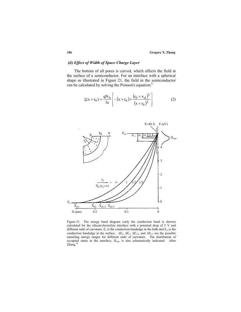
Gregory X. Zhang106
(ii) Effect of Width of Space Charge Layer
The bottom of all pores is curved, which affects the field atthe surface of a semiconductor. For an interface with a sphericalshape as illustrated in Figure 21, the field in the semiconductorcan be calculated by solving the Poisson's equation.8
20
3d0
0b
0rx
xrrx
3
qN)rx( (2)
Figure 21. The energy band diagram (only the conduction band is shown)calculated for the silicon/electrolyte interface with a potential drop of 5 V anddifferent radii of curvature. Ec is the conduction bandedge in the bulk and Ecs is theconduction bandedge at the surface. E , E1, E1/2, and E1/5 are the possibletunneling energy ranges for different radii of curvature. The distribution ofoccupied states at the interface, Dred, is also schematically indicated. AfterZhang.24
0
ro
xd Ecs
ro1 1/2 1/5
∆Ε1/5 ∆Ε1/2 ∆Ε1 ∆Ε∞
Xd (ro=∞)
EcXd∞ Xd1 Xd1/2 Xd1/5
= ∞
X=40 Å E (eV)
Dred
4
3
2
1
0
00.10.2X (µm)
x
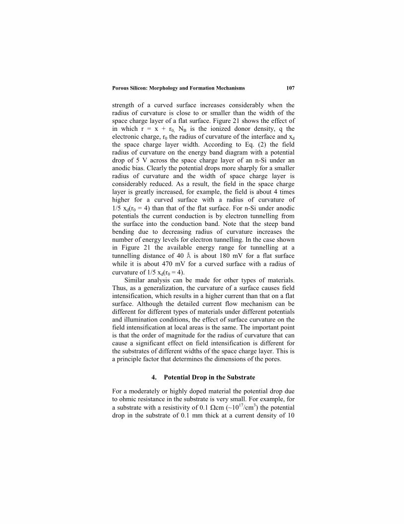
107
strength of a curved surface increases considerably when theradius of curvature is close to or smaller than the width of thespace charge layer of a flat surface. Figure 21 shows the effect ofin which r = x + r0, NB is the ionized donor density, q theelectronic charge, r0 the radius of curvature of the interface and xd
the space charge layer width. According to Eq. (2) the fieldradius of curvature on the energy band diagram with a potentialdrop of 5 V across the space charge layer of an n-Si under ananodic bias. Clearly the potential drops more sharply for a smallerradius of curvature and the width of space charge layer isconsiderably reduced. As a result, the field in the space chargelayer is greatly increased, for example, the field is about 4 timeshigher for a curved surface with a radius of curvature of1/5 xd(r0 = ) than that of the flat surface. For n-Si under anodicpotentials the current conduction is by electron tunnelling fromthe surface into the conduction band. Note that the steep bandbending due to decreasing radius of curvature increases thenumber of energy levels for electron tunnelling. In the case shownin Figure 21 the available energy range for tunnelling at atunnelling distance of 40 Å is about 180 mV for a flat surfacewhile it is about 470 mV for a curved surface with a radius ofcurvature of 1/5 xd(r0 = ).
Similar analysis can be made for other types of materials.Thus, as a generalization, the curvature of a surface causes fieldintensification, which results in a higher current than that on a flatsurface. Although the detailed current flow mechanism can bedifferent for different types of materials under different potentialsand illumination conditions, the effect of surface curvature on thefield intensification at local areas is the same. The important pointis that the order of magnitude for the radius of curvature that cancause a significant effect on field intensification is different forthe substrates of different widths of the space charge layer. This isa principle factor that determines the dimensions of the pores.
4. Potential Drop in the Substrate
For a moderately or highly doped material the potential drop dueto ohmic resistance in the substrate is very small. For example, fora substrate with a resistivity of 0.1 cm (~1017/cm3) the potentialdrop in the substrate of 0.1 mm thick at a current density of 10
nismsPorous Silicon: Morphology and Formation Mecha
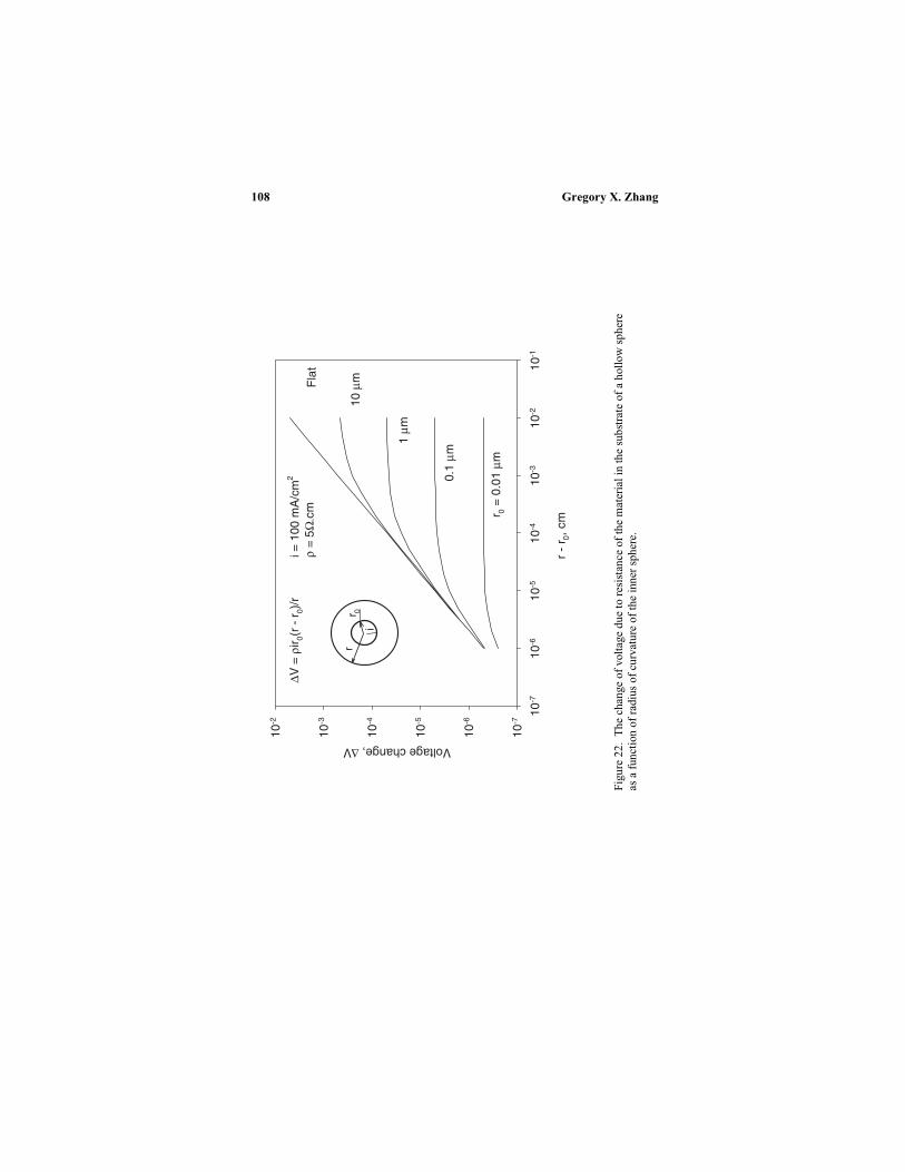
Figu
re 2
2. T
he c
hang
e of
vol
tage
due
to r
esis
tanc
e of
the
mat
eria
l in
the
subs
trat
e of
a h
ollo
w s
pher
eas
a f
unct
ion
of r
adiu
s of
cur
vatu
re o
f th
e in
ner
sphe
re.
Gregory X. Zhang108
r -
r 0, c
m
10-7
10-6
10-5
10-4
10-3
10-2
10-1
Voltage change, ∆V
10-7
10-6
10-5
10-4
10-3
10-2
r 0 =
0.0
1 µm
0.1
µm
1µm
10µmF
lat
i = 1
00 m
A/c
m2
ρ =
5Ω.c
m∆V
= ρ
ir 0(r
- r 0)
/r
rr 0
i

109
mA/cm2 is 0.01 mV, which is insignificant compared to thepotential of millivolt range that is required to significantly affectthe rate of charge transfer process at the interface. However, whenthe resistivity is on the order of 10 cm (~1015/cm3) or larger thepotential drop inside the substrate is in the mV level which startsto affect the distribution of the change of potential in the currentpath.
For a solid between two spherical surfaces shown in Figure22, the resistance can be described by
R = (r-r0)/(4 r0r) (3)
where is the resistivity of the material, r0 is the diameter of theinner sphere and r the outer sphere. The potential drop in thesubstrate, Vs, for a current I = i4 r0
2, where i is the currentdensity on the inner surface, flowing though the solid is thendescribed by
Vs = IR = ir0(r-r0)/r (4)
Figure 22 shows that the potential drop in the material with acurved surface increases non-linearly with increasing distancefrom the inner sphere and most of the potential drop occurs withina distance of a few times the diameter of the inner sphere. Also,for the same thickness of the solid the total potential dropincreases with increasing radius of curvature of the inner sphere,reaching the maximum at an infinitely large radius of curvature,that is, a flat surface. The value of the potential drop is in theorder of mV for a inner diameter of 10 µm under the conditionsshown in Figure 22. It will be larger if the current density or theresistivity is higher. Also, the results shown in Figure 22 are for aspherical surface. In the case of curved pore bottoms, which areroughly semi-spherical, the potential drop from individual porebottom into the solid must be significantly larger than that of anisolated sphere because the current flow from one pore overlapswith those from the neighbouring pores.
The results of the above analysis suggest that the formation ofmacro PS on lowly doped materials can be associated with a non-linear potential distribution in the solid of a curved surface due tothe high resistivity of the solid. The formation of two-layer PS on
nismsPorous Silicon: Morphology and Formation Mecha

Gregory X. Zhang110
p-Si indicates that there are two different physical layers in whichthe potential-current relations are sensitive to the radius ofcurvature. The space charge layer of p-Si is thin under an anodicpotential and is associated with the formation of the micro PS.The non-linear resistive effect of the substrate is responsible forthat of macro PS. Also, to have the same change of potential dropin the substrate, Vs, at a given current density, the radius ofcurvature must be smaller for a material of larger resistivityaccording to Eq. (3). This means that the pore diameter decreaseswith increasing resistivity, which agrees with experimentalresults.39
As a further deduction, the effect of high substrate resistivityshould also occur in the case of lowly doped n-Si. However, thewidth of the space charge layer in such a substrate under ananodic potential is on the same order of magnitude as thedimension of the resistive layer. Since macro PS forms on n-Sisubstrate at an anodic potential in the dark, the effect of these twocauses on the diameter of the pores formed on n-Si in the dark arenot distinguishable under normal conditions. If the conditions canbe controlled in such that the pores formed due to the effect of thespace charge layer and that due to the effect of the resistive layerhave a size difference by at least one order of magnitude it wouldbe possible to obtain the PS with two distinct distributions of porediameters on high resistivity n-Si. Such a condition might exist ata low potential (small space charge layer thickness) on a backilluminated n-Si substrate. It might even be possible to obtain thePS with three distinct distributions of pore diameters on a frontilluminated n-Si sample.
5. Surface Lattice Structure
The surface of a single crystal can have different reactivitiesdepending on the orientation of the surface. For example, thedissolution rate of (100) silicon in alkaline solutions can be manyorders of magnitude larger than that of (111) substrate. A majorcause of orientation dependent reactivity is the bonding conditionof surface atoms. Characteristically, the silicon atoms on (111)surface have three bonds connecting to the substrate lattice whilethose on (100) surface have only two and are thus have weakerattachment to the surface compared to those on (111) surface.99
111
Also, a real surface has atomic structures associated withroughness and defects and thus the atoms at these latticestructures have different bonding conditions, some are similar tothose on a (100) surface in terms of bonding characteristics; someare similar to a (111) surface and others are in between. Thus, areal surface may have varying degrees of reactivity determined bythe concentration of the active atoms, which is a function oflattice structure determined by orientation, roughness, and typeand density of defects.
The rate of an electrode reaction is a function of threeprinciple types of species: charge carriers on the surface, activesurface atoms and reactant species in the solution as illustrated inFigure 23. That is, r [h]*[Siactive]*[A]. Carrier concentration andreactant concentration do not, in general, depend on surfaceorientation while active surface atoms may be a function ofsurface orientation. Anisotropic effect occurs when the ratedetermining step depends on the active surface atoms that varywith crystal orientation of the surface. On the other hand,reactions are isotropic when the concentration of active surfaceatoms is not a function of surface orientation or when the ratedetermining step does not involve active surface atoms.
Figure 23. Schematic illustration of the elemental species involvedin the dissolution reaction of silicon; h: carries inside thesemiconductor, : active silicon atoms an surface and A: etchingspecies in the solution.
nismsPorous Silicon: Morphology and Formation Mecha
Silicon
h
h
h
h
h
h
A
A
A
A
AA
A
active surface atoms
etching species
charge carriers
Solution
Gregory X. Zhang112
The surface, which is rough at the atomic scale, has nodistinct crystallographic character and can be viewed as anamorphous surface as illustrated in Figure 24a. The density ofactive surface atoms on such surface is similar for different crystalorientations. Thus, when the number of atoms at kink sites, stepsand other defects is close to the density of surface atoms, thesurface loses its crystallographic nature. For surfaces of such acondition, the difference in reaction kinetics is small for differentorientations. On the other hand, when the surface is less rough andhas a clear crystallographic character, as shown in Figure 24b, thereaction on the surface is anisotropic when the rate determiningstep involves the surface atoms. When the surface is covered byan amorphous oxide film, the crystallographic nature of thesubstrate is masked and the reaction on such a surface is isotropicas shown in Figure 24c. This is the case for electropolishing ofsilicon electrodes in HF solutions at potentials higher than Vp
where the dissolution is through the formation and dissolution ofsilicon oxide, which is amorphous in structure.
6. Reactions on the Surfaces of Silicon and Silicon Oxide
There are two basic reactions, that is, direct dissolution of siliconvia reaction (I) and (II) and indirect dissolution through theformation and dissolution of silicon dioxide via reaction (II). Therates of both reactions increase with potential and proceedsimultaneously on the surface of silicon. They compete with eachother in rate and coverage of the surface area, and the relativesurface coverage of the two reactions depends on the potential. Ata low potential the surface coverage of oxide is zero when the rateof reaction (II), which is responsible for the formation of oxide, islow compared to the dissolution rate of the oxide. On the otherhand, the coverage is one and the entire surface is covered with anoxide film when the rate of reaction (II) is much higher than thedissolution rate of oxide. Between the two extremes the surface ispartially covered with oxide films at local places where the rate ofreaction (II) equals the oxide dissolution rate. At low potentialsthe oxide formation rate is low compared to the dissolution rateand the surface is not covered by an oxide film. Thus, dependingon the radius of curvature the bottom of a pore may be covered byan oxide film with varying thickness as shown in Figure 25.

Figu
re 2
4. S
chem
atic
illu
stra
tions
of
the
cond
ition
s of
sur
face
lat
tice
stru
ctur
e: (
a) a
mor
phou
s-lik
e su
rfac
e w
ith
no i
dent
ity
of o
rien
tati
on,
(b)
surf
ace
wit
h ki
nks,
ste
ps a
nd t
erra
ces
char
acte
rist
ic o
f ce
rtai
n cr
ysta
lline
ori
enta
tion
and
(c)
sur
face
with
no
iden
tity
of t
he la
ttic
e st
ruct
ure
of t
hecr
ysta
l due
to th
e co
vera
ge o
f an
am
orph
ous
oxid
e fi
lm.
nismsPorous Silicon: Morphology and Formation Mecha 113
(a)
(b)
(c)
Ox
ide f
ilm

Gregory X. Zhang114
Figure 25. Schematic illustration of current variation andcoverage of silicon oxide on the surface of a pore bottom.
Such reactions processes are responsible for the transitionfrom PS formation to electropolishing with increasing potential astypically revealed in an i-V curve.18 PS formation can occur whenthe surface is not or only partially covered by oxide. Once thewhole surface is covered with an oxide film further reaction canonly proceed through the formation of oxide followed by itsdissolution. Further increasing the potential will only result in anincrease of oxide film thickness. On the other hand, increasing HFconcentration will increase the dissolution rate of oxide. Thepresence of oxide on the silicon surface in the PS formationregion and its increase with potential have been experimentallyobserved.98
is
it
θ
SiO2
i
V
ib
is
= itcosθ + i
b
Φ
115
When the surface is completely covered by an oxide film,dissolution becomes independent of the geometric factors such assurface curvature and orientation, which are responsible for theformation and directional growth of pores. Fundamentally, unlikesilicon, which does not have an atomic structure identical indifferent directions, anodic silicon oxides are amorphous in natureand thus have intrinsically identical structure in all orientations.Also, on the oxide covered surface the rate determining step is nolonger electrochemical but the chemical dissolution of the oxide.1
7. Distribution of Reactions and their Rates on Pore
Bottoms
For a stably growing PS the reactions and the rates are differenton the pore walls and on the pore bottoms. Furthermore, they aredifferent at different positions of a pore bottom due to thedifference in the radius of curvature. The current is the largest atthe pore tip because there the radius of curvature is the smallest. Itdecreases from the pore tip to the pore wall as radius of curvatureincreases. On the other hand, since the reactions depend on thecurrent density, for a given condition, direct dissolution of silicondominates at a relatively low current range while oxide formationand dissolution dominate at a higher current range. Thus, oxideformation and dissolution tend to occur at the pore tips at a lowerpotential than at the side of the pore bottom. There is adistribution of the kind of reactions along the pore bottom.
For a pore to propagate under a steady state the currentdensity on the side of the pore bottom, is, and that at the pore tip,it, as illustrated in Figure 25 have the relation.
is = it cos + ib (5)
in which ib is the extra current mostly due to the anisotropic effectand is responsible for the formation of side pores. The currentdensity at different sites on the bottom depends on . It is thelargest at the tip where = 0, and is the smallest on the boundaryof the bottom where = 90o. Such a distribution of current densityis provided by the distribution of radius of curvature along thepore bottom, which determines the field at the silicon surface andthe nature of the reactions. For different HF concentrations and
nismsPorous Silicon: Morphology and Formation Mecha

Gregory X. Zhang116
potentials the current density distribution on the pore bottom isdifferent and so is the shape of the pore bottom. When the porebottom is curved to such an extent that the current densitydistribution on the pore bottom for a given HF concentration and agiven potential satisfies Eq. (5), pores will propagate stably.
(i) Phases in Current Path
As illustrated in Figure 26, which is a varied presentation fora single pore from the scheme shown in Figure 19, there are fivepossible phases in the current path in which significant potentialdrops may occur. The distribution of the applied potential in thedifferent phases of the current path depends on doping type andconcentration, HF concentration, current density, potential,illumination intensity and direction. The phases in the current path
Figure 26. Potential drops along the current path in a pore; VSi =potential drop in silicon substrate, Vs = potential drop in the spacechange layer Vox = potential drop in oxide VH = potential drop in theHelmholtz layer, Vel = potential drop in electrolyte.
∆Vs
∆Vox
∆VSi
∆VH
∆Vel
∆ Vapp
= ∆ Vsi
+ ∆ Vs
+ ∆ Vox
+ ∆ VH
+ ∆ Vel
117
that take large portions of the change in the applied potential,have the consequence of changing current distribution along thepore bottoms, and thus affect the morphology of PS.
The resistance of the electrolyte causes a potential drop that islinearly distributed in the electrolyte inside the pores and thusdoes not have an effect on the current distribution on the porebottom. However, the potential drop in the electrolyte has animportant effect in maintaining the flat growth front of the PSlayer as will be discussed later.
For moderately doped substrates, when the surface is free ofoxide the change of potential is mostly dropped in the spacecharge layer and in the Helmholtz double layer. The reactions arevery sensitive to geometric factors. The reaction that is kineticallylimited by the processes in the space charge layer is sensitive toradius of curvature, while that limited by the processes in theHelmholtz layer is sensitive to the orientation of the surface.Depending on the relative effect of each layer the curvature effectversus anisotropic effect can vary.
When the pore bottom is covered by an oxide, the change ofapplied potential occurs almost completely in the oxide due to thevery high resistance of the oxide. The rate of reactions is nowlimited by the chemical dissolution of the oxide on the oxidecovered area. When the entire pore bottom is covered with anoxide the rate of reaction is the same on the entire surface of thepore bottom. As a result, the bottom flattens and the condition forPS formation disappears. The change of oxide coverage on thepore bottom can also occur when diffusion of the electrolyteinside deep pores becomes the rate limiting process. Since thecurrent at which formation of an oxide occurs increases with HFconcentration, a decreased HF concentration at pore bottom due tothe diffusion effect can result in the formation of an oxide on thepore bottom of a deep pore at a condition that does not occur inshallow pores.
When the resistance of the substrate is high and a significantamount of potential is dropped in the substrate, the potential dropmay not be uniform along a curved pore bottom due to the non-linear potential distribution on the material surrounding thebottom. Formation of macro PS on lowly doped materialsbecomes possible under such a condition.
nismsPorous Silicon: Morphology and Formation Mecha

Gregory X. Zhang118
8. Formation Mechanisms of Morphological Features
Formation of PS is due to preferential dissolution of a siliconsurface; the rate is larger at some areas of the surface relative toothers. Such relative rates with respect to the spatial position ofthe areas, on which these processes occur, are determined more bythe relative nature and less by the absolute nature of the physicaland chemical dimensions and events. Specifically, the relativenature of the following aspects is important in determining themorphology of PS:
1. Radius of curvature relative to the thickness of spacecharge layer
2. Relative depletion of carriers at pore tips to wall region3. Relative dissolution rate on the (100) surface to that on
the (111) surface4. Density of surface atoms at steps and kinks relative to
surface atomic density5. Relative contribution of the preferential dissolution along
direction of carrier source versus that along <100>direction
6. Relative growth rate of the side pores to that of the mainpores
7. Change of profile of pore bottom due to randomperturbations relative to pore size
8. Formation rate of oxide film relative to its dissolutionrate
9. Rate of direct dissolution of silicon relative to indirectdissolution via oxide formation and dissolution
10. Relative share of potential change among the phasesalong the current path
11. Potential drop in electrolyte within a pore relative tothose within the surrounding pores
12. Distance between surface and source of holes relative tothickness of space charge layer
(i) Pore Diameter and Interpore Spacing
Pore diameter and interpore spacing are determined by twolarge groups of factors: those that affect carrier density on thesurface of a pore bottom and those that affect only the distribution

119
of the reactions. The first group of factors include doping type andconcentration, potential, and illumination direction. The secondgroup of factors include current density, HF concentration, andillumination frequency and intensity.
Except for the macro PS on lowly doped p-Si, both the porediameter and wall thickness are largely determined by thethickness of the space charge layer. Thus, in general, porediameter has the same order of magnitude as the thickness ofspace charge layer. Wall thickness is generally less than twice thespace charge layer thickness. Because of the overlapping of thetwo space charge layers the wall region is depleted of carriers andis thus not conductive. If the wall thickness is larger than twicethe space charge layer thickness the walls are not depleted ofcarriers and dissolution can still occur to form new pores on thewalls. Under certain conditions such as backside illumination andsurface patterning for n-Si, pore walls can be much thicker thantwice the space charge layer thickness because of the favourableposition of pore tips for the photo holes generated at the backside.
For a PS formed for controlled space charge layer thickness,the actual wall thickness depends on the relative dissolution ratesbetween the edge of a pore bottom (see Figure 25) and the tip thatis between ib and it. If ib is comparable to it, significant dissolutionoccurs at the edge of the pore bottom before the pore tippropagates far away. This will result in a thin wall or even no wallat all. On the other hand, if ib is very small compared to it, thepore tip will propagate relatively fast so that, before muchdissolution occurs on the edge of the pore bottom, the edge hasalready moved into the wall region where dissolution is virtuallystopped due to lack of carriers. This will generate relatively thickwalls.
At a given anodic current density, the potential is different fordifferent doping types and concentrations due to different currentconducting mechanisms. The combination of doping and potentialthus provide a wide range of thickness of space charge layer andthus a wide range of pore diameters. For n-Si the space chargelayer and thus the dimension of the pores increases withdecreasing doping concentration and with increasing potential.For p-Si, on the other hand, increasing potential reduces thethickness of the space charge layer and results in smaller pores.However, when doping concentration is lower than a certain level,
nismsPorous Silicon: Morphology and Formation Mecha

Gregory X. Zhang120
the effect of substrate resistivity becomes important and formationof macro pores on p-Si can also occur. When this occurs, oneobtains a PS with two distributions of pores with a micro PS layeron the surface of macro pores.
It needs to be pointed out that formation of macro pores canalso occur on moderately or highly doped p-Si in the transitionregion (see Figure 4). Formation of macro pores on p-Si in thetransition region was first noted on highly doped p-Si in aqueousHF solution18 and was recently more systematically investigatedin various non-aqueous solutions for moderately doped p-Si.55
The macro pores formed in the transition region (near the limit ofconditions for PS formation) may not be consistent with respect tosize and depth from area to area as the coverage of PS may not beuniform on the surface. Also, the pores formed in this regiongenerally have very thin walls relative to the size of pores. Theformation of such macro pores can be viewed as a dimensionaltransition from pores of small radius of curvature in theexponential region to the flat surface that has an infinite radius ofcurvature. The formation of such large pores is related to theincreased coverage of oxide on pore bottoms from the exponentialregion to electropolishing region. Since formation and dissolutionof oxide strongly depend on the amount of water in theelectrolyte, the condition for occurrence of the transition regionand formation of macro pores on p-Si can greatly vary with typeof solution as reported recently.55
Under front illumination on n-Si, photo carriers aregenerated from the surface to the depth of penetration determinedby the wavelength of the light. The part of the space charge layerthat has a field effect on the photo carriers varies from almost zeroto the full thickness of the space charge layer. Correspondingly,the size of pores and wall thickness for the PS formed underillumination may vary from zero (i.e., corrosion of PS) to thatcomparable to the thickness of the space charge layer, resulting ina fractal-like PS structure.
When the current is larger than certain value, at which oxidestarts to form at the tip of pores, increasing current density willincrease the coverage of the oxide film on the pore bottom. Insuch a case the relative change in the current at the pore tip it/it
with an increase in the current in the pore, i, is less than that atthe side of the pore bottom, is/is, that is, it/it < is/is. The

121
curvature of the pore bottom will increase resulting in larger poresand thinner walls. On the other hand, when the current isrelatively small so that the current density at the pore tips is stillmuch less than that required for the formation of oxide, anincrease in applied current density will cause a relatively largerincrease at the tip than on the side of the pore bottom (The slopeof an i-V curve in this current range increases with increasingcurrent density.), that is, it/it > is/is. As a result, the pore bottombecomes sharper with increasing current density. On the otherhand, increasing the concentration of HF increases the dissolutionrate of oxide, which in turn increases the critical current density atwhich the surface is covered by oxide. As a result, the poresbecome smaller and walls become thicker with increasing HFconcentration.
(ii) Initiation of Pores
A silicon surface, no mater how well it is prepared, is notperfectly flat at the atomic scale, but has surface defects such assurface vacancies, steps, kinks sites, and dopant atoms. Thedissolution of the surface is thus not uniform but modulated at theatomic scale with higher rates at the defects and depressed sites.The micro roughness of the surface will increase with the amountof dissolution due to the sensitivity of the reactions to surfacecurvature associated with the micro depressed sites. These sites,due to the higher dissolution rates, will evolve into pits andeventually into pores. Depending on the condition, a certainamount of dissolution is required before the initiation of pores onall types of materials.
The pores so initiated are very small in size but large innumber due to the nature of surface defects. However, for the bulkPS formed under a steady state at a given anodization condition,the morphology has determined characteristics in terms of poresize, density, branching etc. Thus, the tiny pores initiated on thesurface are not stable but tend to grow into the size required forsuch bulk PS. As the pores propagate into the bulk, some growgradually in size while some vanish. The thickness of theinitiation phase is comparable to the diameter of the pores grownat the steady state. Thus, the initiation layer is very thin for amicro PS and relatively thick for a macro PS.
nismsPorous Silicon: Morphology and Formation Mecha
Gregory X. Zhang122
Although surface defect sites are involved in the initiation ofpores they do not determine the density and dimension of thepores in the bulk PS. The bulk morphology of PS is determined bythe property of semiconductors and anodization conditions.However, under certain conditions, such as using surfacepatterning to generate initiation sites, the bulk PS morphology canbe controlled to some extent.
(iii) Flatness of the Growth Front of PS
The growth front of a PS layer is generally flat and parallel tothe initial surface of the substrate, meaning that the pores, whichmay have a range of diameters and shapes, propagate atessentially the same rate. This is due to the effect of electrolyteresistance within individual pores. The potential drop in theelectrolyte within the pores, Vel, plays the critical role ofmaintaining the same growth rate for different pores. For a pore oflength, l, the potential drop in the electrolyte with a resistivity, ,inside the pore at a current density i is Vel = i* *l. Vel isindependent of pore diameter and shape but depends on onegeometric factor, that is, the length of the pore. Assume one poreis significantly ahead of the surrounding pores, i will increase dueto the favourable position of the pore bottom. This will thenincrease the potential drop inside the pore, Vel, which in turnwill result in a reduction of the potential available for other phasesin the current path. The reduction of the potential in other phaseswill then reduce the current density and slow down the growth ofthis particular pore. Thus, due to such a process individual porescan only grow at the same rate and, as a result, the growth front ofa PS layer is flat.
(iv) Orientation and Branching of Pores
Orientation, branching and straightness of pores are related tosimilar factors, namely source of holes and anisotropic effect.Orientation of pores can be explained based on the currentdifference between (100) and (111) orientations,
i<100> = i<100> – i<111>, and the difference between currentdensities on the pore bottoms of main pores and on side pores,ihole, main and ihole, side, as shown in Figure 27. ihole, side is smaller than

123
Figure 27. Current components at the tips of main pores and side pores.
ihole, main due to the unfavourable geometric location. At the tip ofmain pores, the total current density can be expressed as
it, main = ihole, main + i<100> (6)
while at the tips of side pores the current density is
it, side = ihole, sidecos + i<100>sin (7)
nismsPorous Silicon: Morphology and Formation Mecha
∆ i<100>
iholes, side
<100>
itip, side
θ
Main pore
Side pore
iholes, main
∆ i<100>
itip, mian
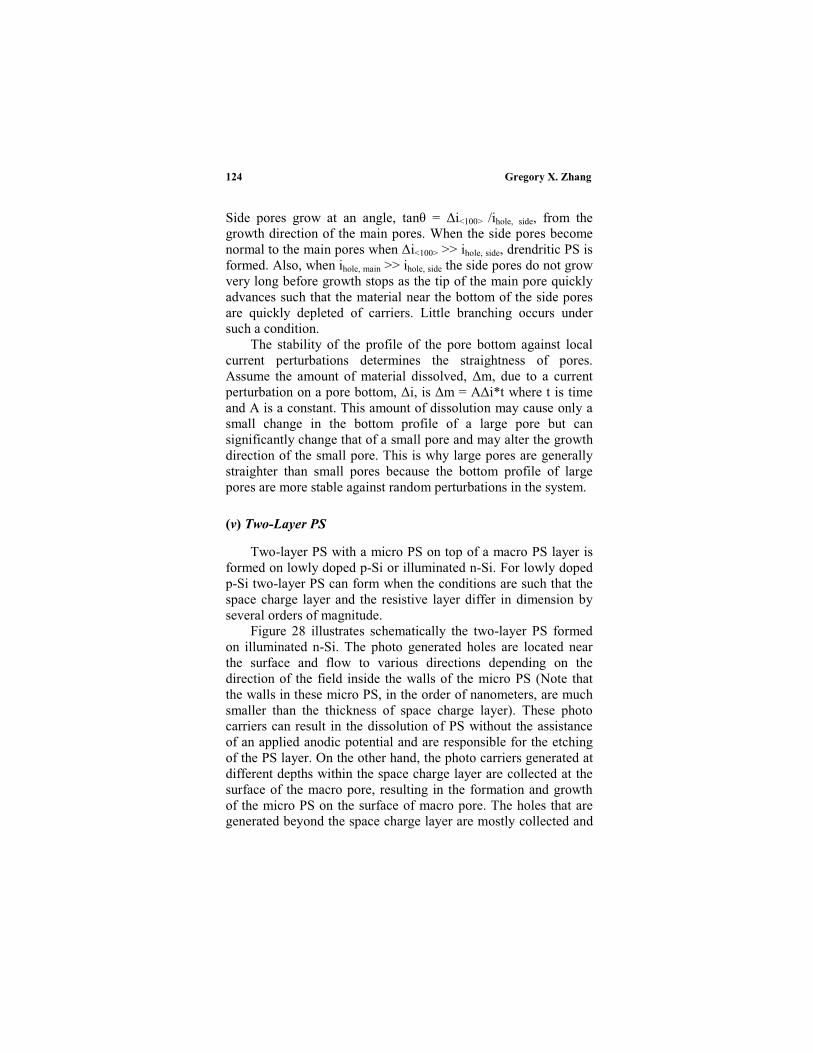
Gregory X. Zhang124
Side pores grow at an angle, tan = i<100> /ihole, side, from thegrowth direction of the main pores. When the side pores becomenormal to the main pores when i<100> >> ihole, side, drendritic PS isformed. Also, when ihole, main >> ihole, side the side pores do not growvery long before growth stops as the tip of the main pore quicklyadvances such that the material near the bottom of the side poresare quickly depleted of carriers. Little branching occurs undersuch a condition.
The stability of the profile of the pore bottom against localcurrent perturbations determines the straightness of pores.Assume the amount of material dissolved, m, due to a currentperturbation on a pore bottom, i, is m = A i*t where t is timeand A is a constant. This amount of dissolution may cause only asmall change in the bottom profile of a large pore but cansignificantly change that of a small pore and may alter the growthdirection of the small pore. This is why large pores are generallystraighter than small pores because the bottom profile of largepores are more stable against random perturbations in the system.
(v) Two-Layer PS
Two-layer PS with a micro PS on top of a macro PS layer isformed on lowly doped p-Si or illuminated n-Si. For lowly dopedp-Si two-layer PS can form when the conditions are such that thespace charge layer and the resistive layer differ in dimension byseveral orders of magnitude.
Figure 28 illustrates schematically the two-layer PS formedon illuminated n-Si. The photo generated holes are located nearthe surface and flow to various directions depending on thedirection of the field inside the walls of the micro PS (Note thatthe walls in these micro PS, in the order of nanometers, are muchsmaller than the thickness of space charge layer). These photocarriers can result in the dissolution of PS without the assistanceof an applied anodic potential and are responsible for the etchingof the PS layer. On the other hand, the photo carriers generated atdifferent depths within the space charge layer are collected at thesurface of the macro pore, resulting in the formation and growthof the micro PS on the surface of macro pore. The holes that aregenerated beyond the space charge layer are mostly collected and
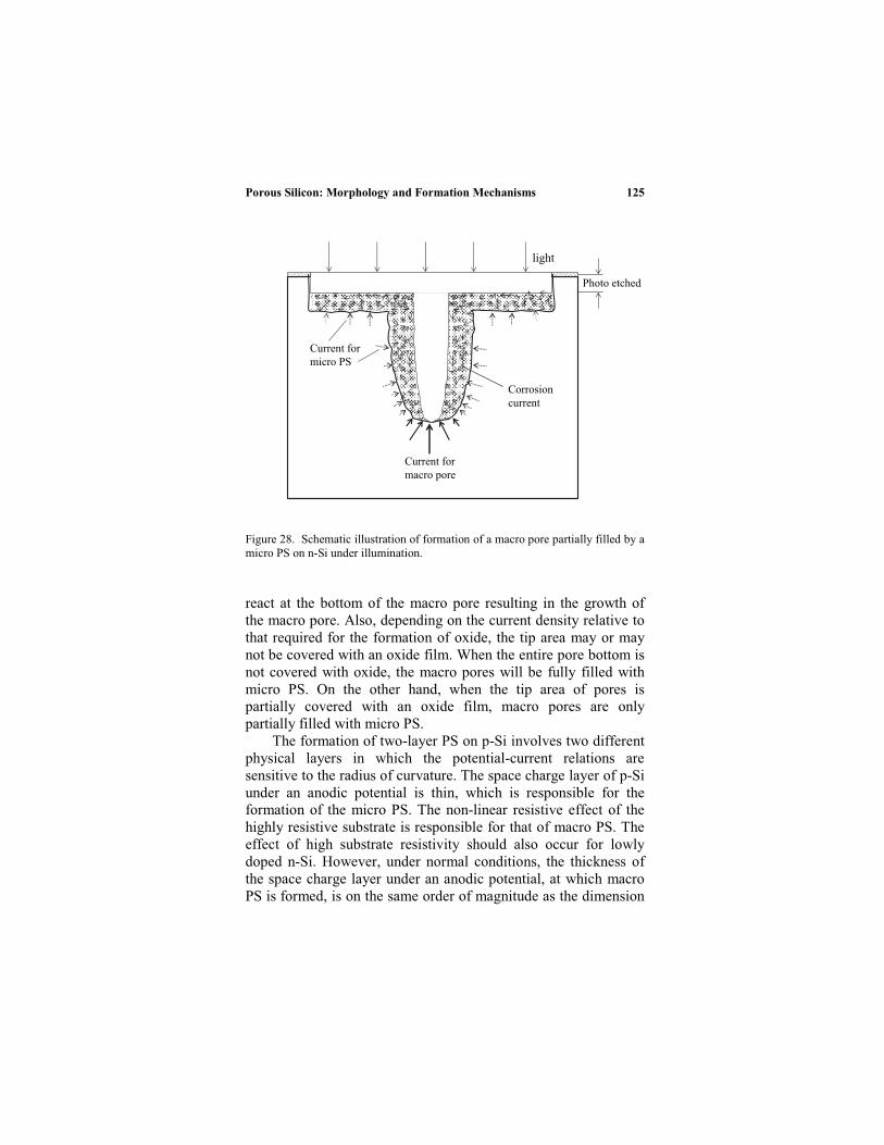
125
Figure 28. Schematic illustration of formation of a macro pore partially filled by amicro PS on n-Si under illumination.
react at the bottom of the macro pore resulting in the growth ofthe macro pore. Also, depending on the current density relative tothat required for the formation of oxide, the tip area may or maynot be covered with an oxide film. When the entire pore bottom isnot covered with oxide, the macro pores will be fully filled withmicro PS. On the other hand, when the tip area of pores ispartially covered with an oxide film, macro pores are onlypartially filled with micro PS.
The formation of two-layer PS on p-Si involves two differentphysical layers in which the potential-current relations aresensitive to the radius of curvature. The space charge layer of p-Siunder an anodic potential is thin, which is responsible for theformation of the micro PS. The non-linear resistive effect of thehighly resistive substrate is responsible for that of macro PS. Theeffect of high substrate resistivity should also occur for lowlydoped n-Si. However, under normal conditions, the thickness ofthe space charge layer under an anodic potential, at which macroPS is formed, is on the same order of magnitude as the dimension
nismsPorous Silicon: Morphology and Formation Mecha
light
Current for
macro pore
Current for
micro PS
Corrosion
current
Photo etched
Gregory X. Zhang126
of the resistive layer. The effect of these two different causes onthe pore diameter is thus not normally distinguishable. If theconditions can be controlled such that the pores formed due to theeffect of the space charge layer and those formed due to the effectof the resistive layer have a size difference by at least one order ofmagnitude it could be possible to obtain two-layer PS on n-Si.
For macro pores at a stable growth condition, the distributionof current density on the surface of an individual pore bottom isbell-like as shown in Figure 29a. For micro PS, the pores tend togrow in a zigzag fashion and the distribution of current at thedissolution front of PS is highly modulated across the surface asillustrated in Figure 29b. For two-layer PS, in which macro porescan be filled or partially filled with micro PS, the current profilesare illustrated in Figure 29c and 29d. The bell-shape distributionof the current responsible for growth of macro pores is consistedof fine modulations of the current responsible for growth of microPS. When the current densities are such that no oxide occurs onany area of the pore bottom the macro pore is fully filled by microPS. On the other hand, when the current density is such that oxideforms at the tip, the macro pore is only partially filled by microPS.
(vi) Dissolution of PS During its Formation
The dissolution of PS during PS formation may occur in thedark or under illumination. Both are essentially corrosionprocesses, by which the silicon in the PS is oxidized and dissolvedwith simultaneous reduction of the oxidizing species in thesolution. The material in the PS, which is distant from thegrowing front is little affected by the external bias due to the highresistivity of PS and is essentially at the open circuit potential(OCP). Such corrosion process is responsible for the formation ofmicro PS of certain thickness (stain film) in HF solutionscontaining oxidants under an unbiased condition.
Because the dissolution of silicon in HF solution requiresholes, the corrosion rate of silicon in HF solutions at OCP is verylow due to the unavailability of holes. But due to the large surfacearea of PS, the amount of dissolution still has a significant effecton the density of PS (e.g., PS density decreases with increasingPS thickness).
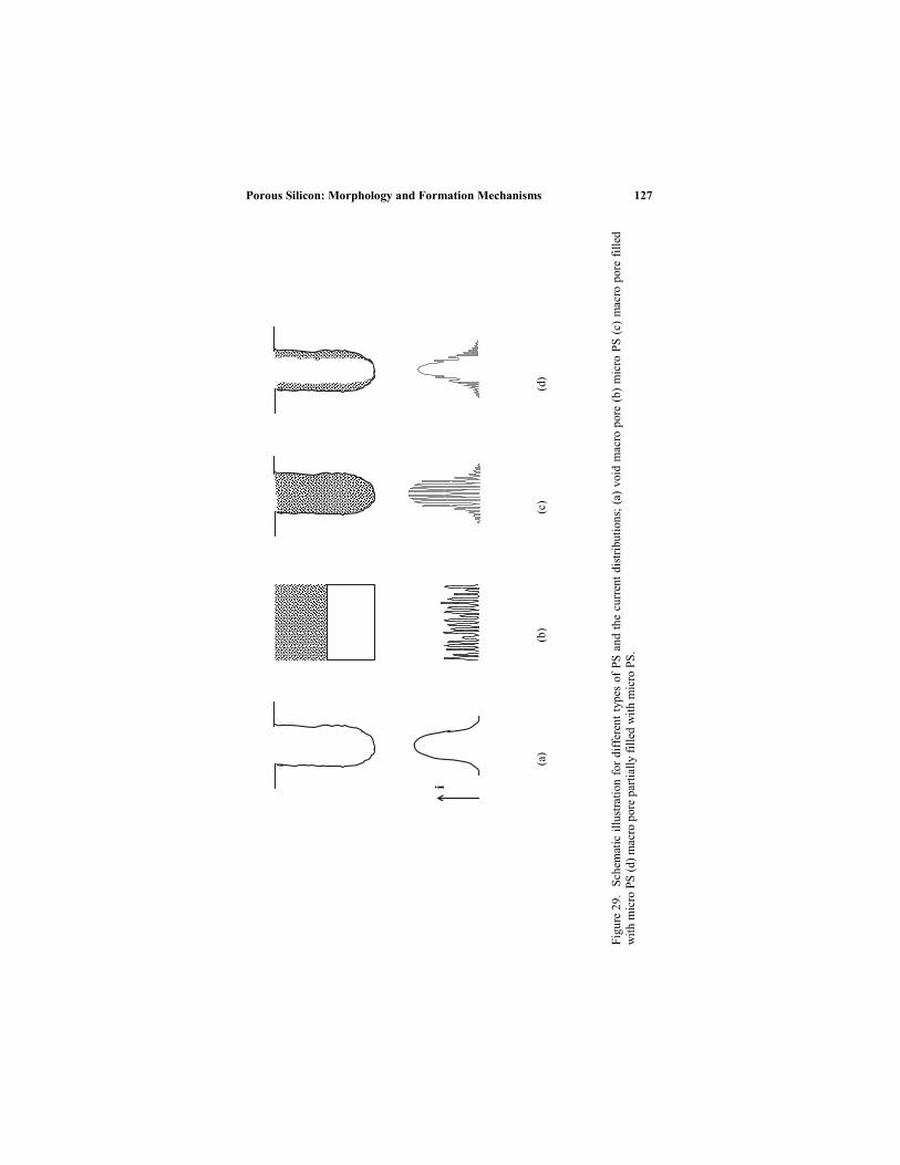
Figu
re 2
9. S
chem
atic
illu
stra
tion
for
diff
eren
t ty
pes
of P
S an
d th
e cu
rren
t di
stri
buti
ons;
(a)
voi
d m
acro
por
e (b
) m
icro
PS
(c)
mac
ro p
ore
fille
dw
ith
mic
ro P
S (d
) m
acro
por
e pa
rtia
lly f
ille
d w
ith
mic
ro P
S.
nismsPorous Silicon: Morphology and Formation Mecha 127
i
(a)
(b)
(c)
( d)

Gregory X. Zhang128
Illumination generates holes within the material of PS andcauses photo corrosion of PS that is much faster than that in thedark. Depending on illumination intensity and time, the pore wallsin a PS can be thinned to various extents by the photo inducedcorrosion. This corrosion process is responsible for the etchedcrater between the initial surface and the surface of PS asillustrated in Figure 28. It is also responsible for the fractalstructure of the micro PS formed under illumination.
V. SUMMARY
This chapter provided a conceptual analysis of the various aspectsof morphology and formation mechanisms of porous silicon basedon available information on the fundamental reaction processes onthe silicon/electrolyte interface. According to the globalmechanistic scheme described, the diverse types of PS can becategorized into three groups: 1) space charge layer controlled.This includes all PS except for the macro PS formed on p-Si. Thediameter of the pores in these PS types is comparable to the widthof space charge layer; 2) substrate resistance controlled. Thisincludes the macro PS formed in lowly doped p-Si and possiblyon lowly doped n-Si (a prediction); 3) photo carrier controlled.This includes all micro PS in single and two-layer PS formedunder illumination.
Some morphological features of porous silicon in relation toformation condition as defined by the kinetics according tocurrent and HF concentration are illustrated Figure 30. The linesdefining the regions are determined by the nature of the reactionsand are independent of the doping type and concentration (seeFigure 4). One important factor governing the change of oneregion to the other is the formation and coverage of an anodicoxide film on the surface. The coverage of oxide on the surfaceincreases from zero in PS region A to only at pore tips in PSregion B to part of the surface in the transition region to fullcoverage in the electropolishing region.
Formation of porous silicon is an anodic dissolution process,which consists of carrier transport in the semiconductor,electrochemical reactions at the interface, and mass transport ofthe reactants and reaction products in the electrolyte. There are a

Figu
re 3
0. C
ondi
tion
s fo
r th
e fo
rmat
ion
of v
ario
us m
orph
olog
ical
fea
ture
s of
PS.
nismsPorous Silicon: Morphology and Formation Mecha 129
PS
regi
on B
Fo
rmati
on
of
ox
ide o
n p
ore
tip
s
An
iso
tro
pic
ity
red
uces w
ith
in
cre
asin
g i
, V
Φ in
cre
ases w
ith V
W r
educes w
ith V
Po
re d
en
sit
y i
ncre
ases w
ith
V
Macro
PS
on n
+, p
+
PS
regi
on A
No
ox
ide f
orm
ati
on
An
iso
tro
pic
ity
in
cre
ase w
ith
in
cre
asin
g i
, V
Both
Φ, W
incre
ases w
ith V
Po
re d
en
sit
y r
ed
uces w
ith
V
Den
dri
tic P
S f
orm
ati
on
po
ssib
le
Tra
nsit
ion
regi
onF
orm
ati
on
of
ox
ide o
n c
urv
ed
are
a
Part
ial
covera
ge a
nd n
on-u
nif
orm
PS
Macro
pore
s
Ele
ctro
plis
hing
reg
ion
Co
mp
lete
ox
ide c
ov
era
ge
No P
S f
orm
ati
on
Unif
orm
dis
solu
tion
Lit
tle a
nis
otr
op
icit
y
iV
Ox
ide
log
[HF
]
log
i
Incr
easi
ng oxid
e co
verag
e

Gregory X. Zhang130
number of reactions involved at the interface and these reactionsconsist of several steps and sub-reactions. At any given time, thedissolution kinetics can be controlled by any one or several ofthese steps. The distribution of reactions along a pore bottomunder a steady state condition during pore propagation must besuch that pore walls are relatively less active than the pore tip.Then, the dissolution reactions are concentrated at the pore tip toresult in the preferential dissolution and the formation of pores.The formation of pores is the consequence of spatially andtemporally distributed reactions.
The fundamental reason for the uneven distribution ofreactions is that the rate of electrochemical reactions on asemiconductor is sensitive to the radius of curvature of thesurface. This sensitivity can either be associated with thethickness of the space charge layer or the resistance of thesubstrate. Thus, when the rate of the dissolution reactions dependson the thickness of the space charge layer, formation of pores canin principle occur on a semiconductor electrode. The specificporous structures are determined by the spatial and temporaldistributions of reactions and their rates which are affected by thegeometric elements in the system. Because of the intricaterelations among the kinetic factors and geometric elements, thedetail features of PS morphology and the mechanisms for theirformation are complex and greatly vary with experimentalconditions.
REFERENCES
1. X. G. Zhang, Electrochemistry of Silicon and Its Oxide, Kluwer Academic,New York, 2001
2. D. R. Turner, J. Electrochem. Soc.,105 (1958) 402.3. A. Uhlir, Jr., The Bell System Technical Journal, March (1956) 333.4. R. Memming and G. Schwandt, Surf. Sci. 4 (1966)109.5. R. L. Meek, J. Electrochem. Soc.,118 (1971) 437.6. M. J. J. Theunissen, J. Electrochem. Soc., 119 (1972) 351.7. Y. Arita and Y. Sunahama, J. Electrochem. Soc., 124 (1977) 285.8. Y. Watanabe, Y. Arita, T. Yokoyama and Y. Lgarashi, J. Electrochem. Soc.,
122 (1975) 1315.9. G. Bomchil, R. Herino, K. Barla and J. C. Pfister, J. Electrochem. Soc.,130
(1983) 1611.10 T. Uganami and M. Seki, J. Electrochem. Soc.,125 (1978) 1339.11. V. Labunov, I. Baranov and V. Bondarenko, Thin Solid Film, 64 (1979) 479.

131
12. M. I. J. Beale, J. D. Benjamin, M. J. Uren, N. G. Chew, and A. G. Cullis, J.Crystal Growth, 73 (1985) 622.
13. S. F. Chuang, S. D. Collins, and R. L. Smith, Appl. Phy. Lett., 55(7), 14August, (1989) 675.
14. R. L. Smith and S. D. Collins, J. Appl. Phy. 71(8), 15 April, (1992) R1.15 R. L. Smith, S. F. Chuang, and S. D. Collins, J. Electronic Materials, 17
(1988) 228.16. T. Unagami, J. Electrochem. Soc., 127 (1980) 476.17 V. P. Parkhutik, L. K. Glinenko, and V.A. Labunov, Surface Technology, 20
(1983) 265.18 X. G. Zhang, S. D. Collins, and R. L. Smith, J. Electrochem. Soc.,136 (1989)
1561.19 V. Lehmann, J. of Electroanalytical Chemistry,140 (1993) 2836.20 V. Lehmann and H. Foll, J. Electrochem. Soc.137 (1990) 653.21 V. Lehmann, Thin Solid Films, 255 (1995) 1.22 V. Lehmann and U. Gosele, Advanced Materials, 4 (1992) 114.23 V. Lehmann and U. Gosele, Appl. Phys. Lett., 58(8), 25 February, (1991)
856.24 X.G. Zhang, J. Electrochem. Soc., 138 (1991) 3750.25 M. H. Al Rifai, M. Christophersen, S. Ottow, J. Carstensen, and H. Foll, J.
Electrochem. Soc., 147 (2000) 627.26 T. Osaka, K. Ogasawara, and S. Nakahara, J. Elechochem. Soc., 144 (1997)
3226.27 C. Levy-Clement, A. Lagoubi and M. Tomkiewicz, J. Electrochem. Soc., 141
(1994) 958.28 C. Levy-Clement, A. Lagoubi, R. Tenne and M. Neumann-Spallart,
Electrochimica Acta, 37(5) (1992) 877.29 A. A. Yaron, S. Bastide, J. L. Maurice and C. L. Clément, J. Luminescence,
57 (1993) 67.30 Y. Arita, Journal of Crystal Growth, 45 (1978) 383.31 C. Levy-Clement, A. Lagoubi, and M. Tomkiewicz, J. Electrochem. Soc.,
141 (1994) 958.32 M. M. Rieger and P. A. Kahl, J. Elechochem. Soc., 142 (1995) 1490.33 E. K. Propst and P. A. Kohl, J. Electrochem. Soc., 141 (1994) 1006.34 E. A. Ponomarev and C. Levy-Clement, Electrochemical and Solid-State
Letters, 1 (1998) 42.35 R. B. Wehrspohn, J. -N. Chazalviel, and F. Ozanam, J.Electrochem. Soc.,
145 (1998) 2958.36 S. Cattarin, E. Pantano, and F. Decker, Electrochemistry Communications, 1
(1999) 483.37 J. -N. Chazalviel, R. B. Wehrspohn, and F. Ozanam, Materials Science and
Engineering, B69-70 (2000) 1.38 R. B. Wehrspohn, F. Ozanam, and J. -N. Chazalviel, J. Electrochem. Soc.,
146 (9) (1999) 3309.39 V. Lehmann and S. Ronnebeck, J. Electrochm. Soc., 146 (1999) 2968.40 J. Carstensen, M. Christophersen, and H. Foll, Materials Science and
Engineering, B69-70 (2000) 23.41 H. Foll, J. Carstensen, M.Christophersen, and G. Hasse, Physica Status
Solidi, a(182) (2000) 45
nismsPorous Silicon: Morphology and Formation Mecha

Gregory X. Zhang132
42 J. Carstensen, M. Christophersen, and H. Foll, Physica Status Solidi, (2000)63.
43 G. Hasse, M. Christophersen, J. Carstensen, and H. Foll, Physica Status
Solidi, a(182) (2000) 23.44 P. Jaguiro, S. La Monica, S. Lazarouk and A. Ferrari, Electrochemical
Society Proceedings, 97-7 (1997) 296.45 A. Valance, Physical Review B, 55 (1997) 9706.46 S. La Monica, P. Jaguiro, and A. Ferrari, Electrochemical Society
Proceedings, 97-7 (1997) 140.47 R. S. Muller and T. I. Kamins, Device Electronics for Integrated Circuits,
John Wiley & Sons, New York, 1977.48 I. Ronga, A. Bsiesy, F. Gaspard, F. Herino, M. Ligeon, and F. Muller, J.
Electrochem. Soc., 138 (1991) 1403.49 F. Gaspard, A. Bsiesy, M. Ligeon, F. Muller, and R. Herino, J. Electrochem.
Soc., 136 (1989) 3043.50 P. C. Searson and X. G. Zhang, J. Electrochem. Soc., 137 (1990) 2539.51 Y. Kang and J. Jorne, J. Electrochem. Soc., 144(9) (1997) 3104.52 M. J. Eddowes, J. Electroanal. Chem., 280 (1990) 297.53 V. A. Burrows, Y. J. Chabal, G. S. Higashi, K. Raghavachari and S. B.
Christman, Appl. Phys. Lett., 53(11) (1988) 998.54 C. M. Gronet, N. S. Lewis, G. Cogan, and J. Gibbons, Proc. Natl. Acad. Sci.
USA, 80 (1983) 1152.55 S. Lust and C. Levy-Clement, J. Electrochem. Soc., 149 (2002) C338.56 E. Peiner, and A. Schlachetzki, J. Elechochem. Soc., 139 (1992) 552.57 J. Rappich and H.J. Lewerenz, Thin Solid Film, 276 (1996) 25.58 J.-N. Chazalviel, M. Etman, and F. Ozanam, J. Electroanal. Chem., 297
(1991) 533.59 P.C. Searson, J.M. Macaulay, and Prokes, J. Electrochem. Soc., 139 (1992)
3373.60 R. Herino, G. Romchil, K. Boala, and C. Bertrand, J. Electrochem. Soc., 134
(1987) 1994.61 I. Ronga, A. Bsiesy, F. Gaspard, F. Herino, M. Ligeon, and F. Muller, J.
Electrochem. Soc., 138 (1991) 1403.62 V. V. Doan and M. Sailor, Science, 256 (1992) 1791.63 M. Christophersen, J. Carstensen, A. Feuerhake, and H. Foll, Materials
Science and Engineering, B69-70 (2000) 194.64 L. Koker and K. W. Kolasinski, Materials Science and Engineering, B69-70
(2000) 132.65 X. G. Zhang, unpublished results.66 R. C. Frye, Mat. Res. Soc. Symp. Proc., 33 (1984) 53.67 M. Guendouz, P. Joubert, and M. Sarret, Materials Science and Engineering,
B69-70 (2000) 43.68 H. Unno, K. Imai, and S. Muramoto, J. Electrochem. Soc., 134 (1987) 645.69 H. Braumgart, R. C. Frye, F. Philipp, and H. J. Leamy, Mat. Res. Soc. Symp.
Proc. 33 (1984) 63.70 O. Teschke, Appl. Phys. Lett., 64(15) (1994) 1986.71 M. I. J. Beale, N. G. Chew, M. J. Uren, A. G. Cullis, and J. D. Benjamin,
Appl. Phys. Lett., 46(1) (1985) 1095.72 H. Sugiyama and O. Nittono, Journal of Crystal Growth, 103 (1990) 156.

133
73 K. D. Legg, A. B. Ellis, J. M. Bolts, and M. S. Wrighton, Proc. Natl. Acad.Sci. USA, 74(10) (1977) 4116.
74 N. Noguchi, I. Suemune, M. Yamanishi, G. C. Hua, and Nobuo Otsuka, Jpn.
J. Appl. Phys., 31 (1992) L490.75 M. Christophersen, J. Carstensen, and H. Foll, Physica Status Solidi, (a) 182,
1 (2000) 45.76 S. -F. Chuang, S. D. Collins, and R. L. Smith, Appl. Phys. Lett., 55(15)
(1989) 1540.77 P. C. Searson, J. M. Macaulay, and F. M. Ross, J. Aapl. Phys., 72(1) (1992)
253.78 T. Osaka, K. Ogasawara, M. Katsunuma, and T. Momma, J. of
Electroanalytical Chemistry, 396 (1995) 69.79 V. Labunov, V. Bondarenko, L. Glinenko, A. Dorofeev and L. Tabulina,
Thin Solid Films, 137 (1986) 123.80 V. Lehmann, R. Stengl, and A. Luigart, Materials Science and Engineering,
B69 (2000) 11.81 V. Lehmann, A. Luigart and V. Corbel, Electrochemical Society
Proceedings, 97-7 (1997) 132.82 C. Gui, M. Elwenspoek, J. G. E., Gardeniers, and P. V. Lambeck, J.
Electrochem. Soc., 145 (1998) 2204.83 E.A. Ponomarev and C. Levy-Clement, Electrochemical Society
Proceedings, 97-7 (1997) 319.84 C. Jäger, B. Finkenberger, W. Jäger, M. Christophersen, J. Carstensen, and
H. Föll, Materials Science and Engineering, B69-70 (2000) 199.85 V. Lehmann and U. Grüning, Thin Solid Films, 297 (1997) 13.86 J. E. A. M. van den Meerakker, R. J. G. Elfrink, F. Roozeboom and J. F. C.
M. Verhoeven, J. Electrochem. Soc., 147(7) (2000) 2757.87 P. Allongue, C. H. de Villeneuve, M. C. Bernard, J. E. Peou, A. Boutry-
Forveille, and C.Levy-Clement, Thin Solid Films, 297 (1997) 1.88 St. Frohnhoff, M. Marso, M. G. Berger, M. Thonossen, H. Luth, and H.
Munder, J. Elechochem. Soc., 142 (1995) 615.89 M. Binder, T. Edelmann, T. H. Metzger, G. Mauckner, G. Goerigk, and J.
Peisl, Thin Solid Film, 276 (1996) 65.90 S. Billat, M. Thonissen, R. Arens-Fischer, M. G. Berger, M. Kruger, and H.
Luth, Thin Solid Films, 297 (1997) 22.91 R. Houbertz, U. Memmert, and R. J. Behm, J. Vac. Sci. Technol. B, 12(6)
(1994) 3145.92 M. Thönissen, M. G. Berger, R. Arens-Fischer, O. Glüger, and H. Lüth, Thin
Solid Films, 276 (1996) 21.93 M. Thönisson, M. G. Berger, R. Arens-Fisher, O. Glück, M. Krüger, and H.
Lüth, Thin Solid Film, 276 (1996) 21.94 S. F. Chuang, S. D. Collins and R. L. Smith, The Technical Digest of the
Solid State Sensor and Actuator Workshop, Hilton Head Island, SC, June 6-9, IEEE, New York, 1988, p.151.
95 S. Ronnebeck, J. Carstensen, S. Ottow, and H. Foll, Electrochemical andSolid State Letters, 2 (2000) 126.
96 S. Bengtsson and L. Engstrom, J. Appl. Phys., 66(3) (1989) 1231.97 A. G. Cullis and L. T. Canham, Nature, 353 (1991) 353.98 A. Belaidi, M. Safi, F. Ozanam, J. N. Chazalviel, and O. Gorochov, J.
Electrochem. Soc., 46 (1999) 2659.
nismsPorous Silicon: Morphology and Formation Mecha
135
3
Modeling Electrochemical Phenomena via
Markov Chains and Processes
Thomas Z. Fahidy
Department of Chemical Engineering, University of Waterloo, Waterloo, Ontario,
Canada N2L 3G1
I. INTRODUCTION
Named after the Russian mathematician Andrei Andreievich
Markov (1856–1922), Markov chains and processes express the
probability evolution of events, whose future, loosely speaking, is
independent of their past. The terminological difference between
the two designations is that Markov chains are related to discrete
events, whereas Markov processes are related to continuous
events. Put simply, Markov chains are discrete Markov processes.
Both have gained prominence in physics, engineering,
management sciences, game theory, etc., and, in general, in the
study of complex processes. A comprehensive survey of historical
background and development, literature and scope of applications
by Tamir1 is highly recommended to the seriously interested
reader (the contents of the book transcend its title!). Fundamental
theory has been presented in the classic texts e.g., by Pugachev,2
Parzen,3 Stark and Woods,4 Rozanov,5 and Sveshnikov.6 Matrix
techniques pertinent to Markov chains have been discussed e.g.,
Modern Aspects of Electrochemistry, Number 39, edited by C. Vayenas et al.,
Springer, New York, 2005.

Thomas Z. Fahidy 136
by Gantmacher,7 and Greenberg.8 References 9-14 form a small,
but illustrative sample of the continuing wide interest in the
subject matter (also manifested by the 392 references listed on the
Internet in early May 2004 under the title of Markov processes).
In the domain of electrochemistry and electrochemical
engineering, the penetration of Markov theory has so far been
rather scant. In an early exploratory study the usefulness of the
Erlang formula (Section II.3) was demonstrated for the analysis of
magnetically enhanced natural convection in electrolysis.15 The
interpretation of spatio–temporal discharge patterns as a
probabilistic function of a Markov process indicates that the latter
is a powerful tool in the analysis of multi–electrode data related to
neuronal spike activity.16 In an investigation of thin film growth
processes dependent on the substrate interaction potential,
Opri an et al.17 used a local Markov chain–based random function
model, where the transition probability matrix describes Brownian
motion in a rectangular lattice in order to produce 2D fractal
patterns. Markov process–based random walks within a lattice
was also used in the simulation of Brownian motion of ions in a
force field,18 for studying the effect of ionic migration and
diffusion on the roughness of electrodeposits: the eventual
disappearance of the influence of initial roughness is a
concomitant conclusion. Random walk/Markov process models
were also applied to diffusion-limited aggregates and electro-
deposition clusters,19-21 diffusion across ion-exchange
membranes,22 and to tank electrolyzers.23
In addition to providing a survey of previous studies, it is also
the purpose of this chapter is to explore new avenues of potential
applications to various electrochemical phenomena. A condensed
theoretical background is first presented, and followed by a
Markovian treatment of selected processes and phenomena of
interest to electrochemists, electrochemical engineers,
electrochemical technologists, and technical managers involved
with electrochemical plants. Multidimensional analysis is
excluded, however, from this essentially whetting the appetite
exercise. Material in Section V relies heavily on author’s personal
(and hitherto unpublished) research. The presentation, although by
no means exhaustive, intends to focus on basic concepts, potential
utility and new horizons, rather than to pursue completeness.
Markov—Modeling of Electrochemical Phenomena 137
II. A CONCISE THEORY OF MARKOV CHAINS AND
PROCESSES
1. Fundamental Notions5,6
of Markov chains
A physical system, occupying states s0, s1, …changes randomly its
state from an initial state at zero time, i.e., a random variable X(t)
of the state undergoes consecutive transitions X(0) X(1)
X(2) … The state is at si (t = 0) with initial probability pi0 =
Pr[X(0) = si ]; i = 1,2,… Then, the transition probability
,...2,1 ; ])(/)1(Pr[ isnXsnXp ijij (1)
yields the probability of the system being at state sj at time or
stage (n + 1), if it was at state si at time or stage (n). This
probability does not depend on time (n). The random process X(t)
is called a Markov chain with stationary random probabilities, or
simply a Markov chain. It follows that the probability pj(n) that
the system will be in the state sj at time (n) (or, equivalently, after
n steps) may be expressed as
0)0( jj pp (2a)
k
kjkj npnpnp ...2,1 ; )1()( (2b)
If, at t = 0 the system is in the state si , then pi0 = 1, pk
0 = 0 for k
i, hence
ijp
ijp
ij
ij
; 0)0(
; 1)0(
(3a)
and
...2,1 ; )1()( npnpnp
k
kjikij (3b)
Thomas Z. Fahidy 138
is the probability that the system will go from state si to state sj in
n steps. The elements p11, p12, p13…form the first row, p21, p22,
p23…form the second row, etc. of the Markov matrix P with the
important characteristic of
P(n) = (P) n ; P(0) = I (4)
where I is the identity matrix. The one-dimensional random walk
is a classical Markov chain.
Working with Markov chains, confusion is bound to arise if
the indices of the Markov matrix are handled without care. As
stated lucidly in an excellent elementary textbook devoted to
finite mathematics,24 transition probability matrices must obey the
constraints of a stochastic matrix. Namely that they have to be
square, each element has to be non-negative, and the sum of each
column must be unity. In this respect, and in order to conform
with standard rules vector-matrix multiplication, it is preferable to
interpret the probability pij as the probability of transition from
state sj to state si (this interpretation stipulates the standard Pp
format instead of the pTP format, the latter convenient for the
alternative si sj interpretation in defining pij) .5,6
If pj(n) pj* as n , then pj
* ; j = 1,2,… describe the final
probability distribution of the system being at state sj . Since as
n , pj(n) = Ppj(n – 1), the limiting probabilities are defined
also by the classical eigenvalue theorem7pj
* = Ppj* with an implied
eigenvalue of unity (Appendix), and the sum of all probabilities
being equal to unity. A tutorial treatment of chemical kinetics25
provides a simple illustration.
Similar to the discrete case, pi0 = Pr[X(0) = si], i = 1,2,…is the
initial probability of the random process being in state si. The
transition probability
...2,1, ; ])(/)(Pr[)( jisXstXtp ijij (5)
expresses the probability that the system is in state sj after a time t,
if it was in state si at time ; this probability is independent of . If
pij(0) = 1 for j = i, and zero for any j i, then
Markov—Modeling of Electrochemical Phenomena 139
k
kjikij jitpptp ,...2,1, ; )()()( (6)
for any arbitrary and t, and
k
jjkjkj ppjtpptp 0)0( ; ,...2,1);()()( (7)
An important case is where the transitional probabilities can be
expressed as pii( t) = 1 – i t and pij( t) = ij (t); j i; i = 1,2,…
with i being the density parameter of transition out of the state si,
and ij the density parameter of transition out of the state si to the
state sj . Defining ii = – i , i = 1,2,…, the transition probabilities
satisfy the forward Kolmogorov (also known as Chapman-
Kolmogorov) equation
...2,1, ; )(/)( jitpdttdp ik
k
kjij (8)
and the backward Kolmogorov equation
k
kjikij jitpdttdp ,...2,1, ; )(/)( (9)
with initial conditions pij(0) = 1, if j = i; zero, if j i. The limiting
probabilities are similar to the Markov chain case in the sense that
tptp jj ;)(lim * (10)
is the probability of the system occupying the state sj at very large
times, independent of the initial probability distribution.
Finally, if a Markov process is in some state s at some
(reference) time t0, and if is the random time required for the
process to leave state s to go to some other state, then the
probability that is larger than some arbitrary time t is given by
0 ; )exp(]Pr[ ttt (11)

Thomas Z. Fahidy 140
where is a non-negative constant. This important theorem
describes the conduct of a service system with exponential
holding times in queuing theory.
2. The Erlang Formula
Taking the limit in Eq. (7) as , and considering the (more
practical) case of a finite number of states m,
i
ijij mjtppp ,...,1 ; )(** (12)
mjp
i
iji ,...,1 ; 0* (13)
If there exist only two states s0 and s1 , it follows from Eq. (13)
that p0*
01 + p1* 11 = 0. It is useful to invoke certain concepts of
queuing theory at this stage, and consider the states as number of
servers handling incoming calls, the arrivals of calls having a
Poisson distribution with parameter . Then, 01 = , and 11 = –µ,
where µ is the density parameter of service. Eq. (13) can further
be written as p0* = µp1
* . If there are two servers (or three states
s0, s1, and s2 where s0 represents the state of no server being
engaged), Eq. (13) can be written as p0*
01 + p1*
11 + p2*
21 = 0.
Given that 01 = ; 11 = –( + µ), and 21 = 2µ, the final form is
( + µ)p1* = p0
* + 2µp2*. In general, the m-server pattern can be
written as
*1
*0 pp (14a)
1,2,1 ; )1()( *1
*1
* mjpjppj jjj (14b)
**1 mm pmp (14c)
From this set, the individual limiting probabilities are obtained by
successive elimination as ;2/)/( ;)/( *0
2*2
*0
*1 pppp
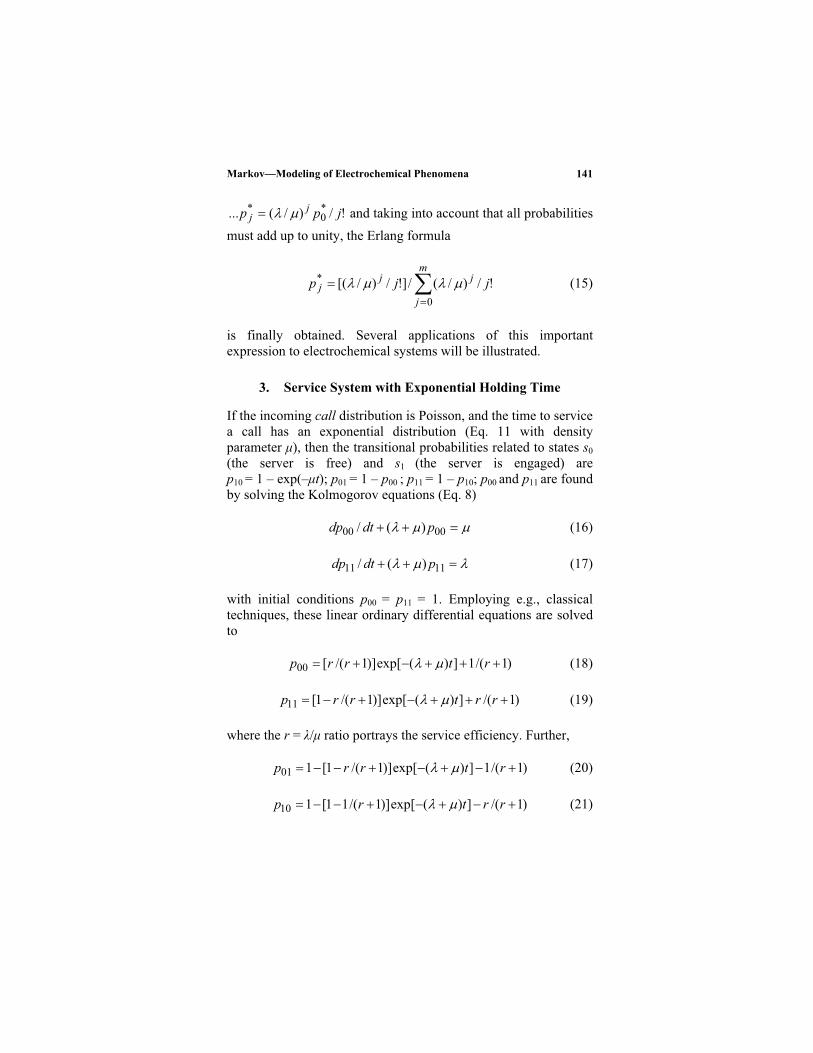
Markov—Modeling of Electrochemical Phenomena 141
!/)/(... *0
* jpp jj and taking into account that all probabilities
must add up to unity, the Erlang formula
m
j
jjj jjp
0
* !/)/(/]!/)/[( (15)
is finally obtained. Several applications of this important
expression to electrochemical systems will be illustrated.
3. Service System with Exponential Holding Time
If the incoming call distribution is Poisson, and the time to service
a call has an exponential distribution (Eq. 11 with density
parameter µ), then the transitional probabilities related to states s0
(the server is free) and s1 (the server is engaged) are
p10 = 1 – exp(–µt); p01 = 1 – p00 ; p11 = 1 – p10; p00 and p11 are found
by solving the Kolmogorov equations (Eq. 8)
0000 )(/ pdtdp (16)
1111 )(/ pdtdp (17)
with initial conditions p00 = p11 = 1. Employing e.g., classical
techniques, these linear ordinary differential equations are solved
to
)1/(1])(exp[)]1/([00 rtrrp (18)
)1/(])(exp[)]1/(1[11 rrtrrp (19)
where the r = /µ ratio portrays the service efficiency. Further,
)1/(1])(exp[)]1/(1[101 rtrrp (20)
)1/(])(exp[)]1/(11[110 rrtrp (21)
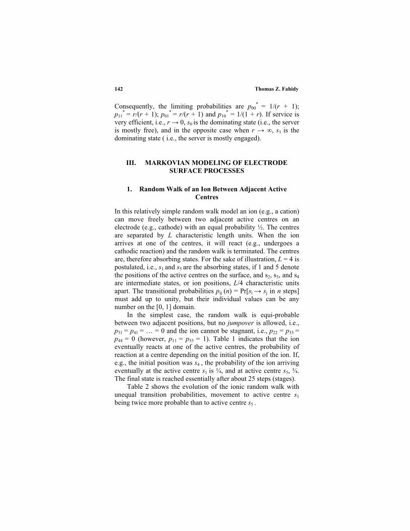
Thomas Z. Fahidy 142
Consequently, the limiting probabilities are p00* = 1/(r + 1);
p11* = r/(r + 1); p01
* = r/(r + 1) and p10* = 1/(1 + r). If service is
very efficient, i.e., r 0, s0 is the dominating state (i.e., the server
is mostly free), and in the opposite case when r , s1 is the
dominating state ( i.e., the server is mostly engaged).
III. MARKOVIAN MODELING OF ELECTRODE
SURFACE PROCESSES
1. Random Walk of an Ion Between Adjacent Active
Centres
In this relatively simple random walk model an ion (e.g., a cation)
can move freely between two adjacent active centres on an
electrode (e.g., cathode) with an equal probability ½. The centres
are separated by L characteristic length units. When the ion
arrives at one of the centres, it will react (e.g., undergoes a
cathodic reaction) and the random walk is terminated. The centres
are, therefore absorbing states. For the sake of illustration, L = 4 is
postulated, i.e., s1 and s5 are the absorbing states, if 1 and 5 denote
the positions of the active centres on the surface, and s2, s3, and s4
are intermediate states, or ion positions, L/4 characteristic units
apart. The transitional probabilities pij (n) = Pr[si sj in n steps]
must add up to unity, but their individual values can be any
number on the [0, 1] domain.
In the simplest case, the random walk is equi-probable
between two adjacent positions, but no jumpover is allowed, i.e.,
p31 = p41 = … = 0 and the ion cannot be stagnant, i.e., p22 = p33 =
p44 = 0 (however, p11 = p55 = 1). Table 1 indicates that the ion
eventually reacts at one of the active centres, the probability of
reaction at a centre depending on the initial position of the ion. If,
e.g., the initial position was s4 , the probability of the ion arriving
eventually at the active centre s1 is ¼, and at active centre s5, ¾.
The final state is reached essentially after about 25 steps (stages).
Table 2 shows the evolution of the ionic random walk with
unequal transition probabilities, movement to active centre s1
being twice more probable than to active centre s5 .

Markov—Modeling of Electrochemical Phenomena 143
Table 1
Elements of the Transition Probability Matrix of a
Unidimensional Equiprobable Random Walk
Model for an Ion Moving on an Electrode Surface;
S1 And S5 are Absorbing States
n = 1 i = 1 i = 2 i = 3 i = 4 i = 5
j = 1 1 0 0 0 0
j = 2 ½ 0 ½ 0 0
j = 3 0 ½ 0 ½ 0
j = 4 0 0 ½ 0 ½
j = 5 0 0 0 0 1
n = 10 i = 1 i = 2 i = 3 i = 4 i = 5
j = 1 1 0 0 0 0 j = 2 0.7344 0.0156 0 0.0156 0.2344
j = 3 0.4844 0 0.0312 0 0.4844
j = 4 0.2344 0.0156 0 0.0156 0.7344
j = 5 0 0 0 0 1
n 25 i = 1 i = 2 i = 3 i = 4 i = 5
j = 1 1 0 0 0 0
j = 2 ¾ 0 0 0 ¼
j = 3 ½ 0 0 0 ½
j = 4 ¼ 0 0 0 ¾
j = 5 0 0 0 0 1
2. Markovian Analysis of Layer Thickness on a Surface
If the service system concept is adapted to a reactive solid surface,
its active centres can be divided into a number of agglomerates or
clusters, and the probability of N clusters being engaged can be
related to the efficiency of the surface via the Erlang formula. The
approach is illustrated by an oxide-thickness-on-wafers problem26
where seven random measurements of oxide layer thickness
obtained under identical experimental conditions are given as
1264, 1280, 1301, 1300, 1292, 1307, 1275 in units. The model
postulates a single- cluster activity responsible for oxide layer
thickness between 1260–1270; two-cluster activity for thickness
between 1270–1280, etc…assigning a total of five clusters to the
entire 1260–1310 range. Alternatively, activity levels labeled 0, 1,
2, … can be envisaged for each layer thickness range. Following
elementary rules of statistical data classification (described in any

Thomas Z. Fahidy 144
Table 2
Elements of the Transition Probability Matrix of a
Unidimensional Unequiprobable Random Walk
Model for an Ion Moving on an Electrode Surface; S1
and S5 are Absorbing States
n = 1 i = 1 i = 2 i = 3 i = 4 i = 5
j = 1 1 0 0 0 0 j = 2 2/3 0 1/3 0 0
j = 3 0 2/3 0 1/3 0
j = 4 0 0 2/3 0 1/3
j = 5 0 0 0 0 1
n = 10 i = 1 i = 2 i = 3 i = 4 i = 5
j = 1 1 0 0 0 0
j = 2 0.9229 0.00867 0 0.00433 0.0641
j = 3 0.7861 0 0.0174 0 0.1965
j = 4 0.5125 0.0173 0 0.00867 0.4615
j = 5 0 0 0 0 1
n 25 i = 1 i = 2 i = 3 i = 4 i = 5
j = 1 1 0 0 0 0
j = 2 0.9333 0 0 0 0.0667
j = 3 4/5 0 0 0 1/5
j = 4 0.5333 0 0 0 0.4667
j = 5 0 0 0 0 1
text on elementary statistics) the cumulative distribution function
is approximated by assigning cumulative frequencies to their
respective class mid-points, and joining these values by a
continuous curve. Cluster efficiency, defined as r = /µ, is
computed via the Erlang formula (Eq. 15), expressed as
N
j
jN jrNrN
0
!//!/]Pr[ (22)
where Pr[N] is obtained as the difference between the values of
the cumulative distribution function evaluated at adjacent class
mid-points. Table 3 demonstrates that the thickness level can be
interpreted in terms of service efficiency, i. e. the faster the
surface activity, the thicker the deposit layer on it. In queuing

Markov—Modeling of Electrochemical Phenomena 145
Table 3
Cluster Efficiency by Erlang’s Formula Applied to the Oxide
Layer Thickness Problem25
Cluster no. N 1 2 3 4 5
Class interval 1260–1270 1270–1280 1280–1290 1290–3000 3000–3100 Pr[N] 0.22 0.15 0.14 0.27 0.22
r = /µ 0.28 0.80 1.54 3.59 4.24
theory, an equivalent statement would be that the faster the
service (or the larger the number of servers available), the larger
the number of clients that can be served.
3. Markovian Interpretation of an Anodic Deposit
Formation Deposit Dissolution Process
Consider an electrode process consisting of the following
(periodic) sequence: an anion is subjected to an anodic reaction
producing a solid deposit on the anode, followed by partial
desorption/re-dissolution from the surface into the electrolyte. In a
Markovian framework, if s1 is the ionic state, and s2 is the surface
deposit state, the transition probabilities p11, p12, p21, p22 define the
probability of the ion remaining in the ionic state, the deposit
desorbing and re-dissolving into the ionic state, the ion
undergoing reaction and forming a deposit, the deposit desorbing
and re-dissolving, the deposit remaining on the surface,
respectively, the indexing according to statements following Eq.
(4).
The system is mathematically trivial if the transitional
probabilities are equally ½, inasmuch as P = Pn , regardless of the
magnitude of n. This would be the case of sustained oscillation
between ionic and deposit state. Table 4 demonstrates the
evolution of the Markov chain in the case of unequal transition
probabilities, in two specific instances. The speed of convergence
to limiting values decreases with the degree of asymmetry in the
P-matrix elements. The limiting values do not depend on the
initial state, inasmuch as they are eigenvector elements related to
the eigenvalue of unity. The complementary eigenvalues of 0 in
the first, and 0.4 in the second instance have no importance, since
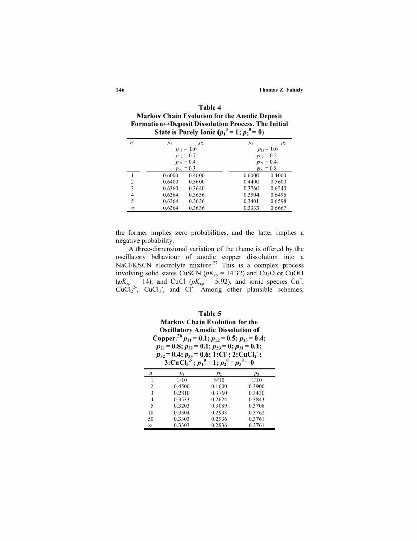
Thomas Z. Fahidy 146
Table 4
Markov Chain Evolution for the Anodic Deposit
Formation Deposit Dissolution Process. The Initial
State is Purely Ionic (p10 = 1; p2
0= 0)
n p1 p2
p11 = 0.6
p12 = 0.7
p21 = 0.4
p22 = 0.3
p1 p2
p11 = 0.6
p12 = 0.2
p21 = 0.4
p22 = 0.8
1 0.6000 0.4000 0.6000 0.4000
2 0.6400 0.3600 0.4400 0.5600
3 0.6360 0.3640 0.3760 0.6240
4 0.6364 0.3636 0.3504 0.6496
5 0.6364 0.3636 0.3401 0.6598
0.6364 0.3636 0.3333 0.6667
the former implies zero probabilities, and the latter implies a
negative probability.
A three-dimensional variation of the theme is offered by the
oscillatory behaviour of anodic copper dissolution into a
NaCl/KSCN electrolyte mixture.27 This is a complex process
involving solid states CuSCN (pKsp = 14.32) and Cu2O or CuOH
(pKsp = 14), and CuCl (pKsp = 5.92), and ionic species Cu+,
CuCl22-, CuCl3
-, and Cl-. Among other plausible schemes,
Table 5
Markov Chain Evolution for the
Oscillatory Anodic Dissolution of
Copper.26
p11 = 0.1; p12 = 0.5; p13 = 0.4;
p21 = 0.8; p22 = 0.1; p23 = 0; p31 = 0.1;
p32 = 0.4; p33 = 0.6; 1:Cl-; 2:CuCl2
-;
3:CuCl32-
; p10= 1; p2
0= p3
0= 0
n p1 p2 p3
1 1/10 8/10 1/10
2 0.4500 0.1600 0.3900
3 0.2810 0.3760 0.3430
4 0.3533 0.2624 0.3843
5 0.3203 0.3089 0.3708
10 0.3304 0.2933 0.3762
50 0.3303 0.2936 0.3761
0.3303 0.2936 0.3761

Markov—Modeling of Electrochemical Phenomena 147
transition from Cl- to CuCl2- and CuCl3
2-, from CuCl2- to Cl- and
CuCl32- , and from CuCl3
2- to Cl- can be postulated. Table 5
illustrates Markov chain evolution with a hypothetical transition
probability array, indicating a slow convergence to the limiting
state. The other two eigenvalues, approximately 0.06 and –0.329
have no significance, since they yield negative and larger – than -
one probabilities.
4. The Electrode Surface as a Multiple Client – Server:
A Markovian View
If an electrode surface is considered to contain a multiple set of
identically functioning single active centres/servers, where each
ion can have a choice of several adjacent servers,28 the probability
that exactly j number of severs is occupied at any given time may
be computed by the Erlang formula (Eq. 15), provided that
numerical values of and µ, or r = /µ are known. From a
practical point of view, two particular states are of interest: s0 ,
where the entire surface is free for an electrode reaction to
proceed, and sm , where the entire surface is covered by the
reaction product; m is the number of active centres, or clusters of
active centres. A small value of r represents either a slow arrival
of ions, or a fast electrode reaction, and vice versa. When r = 1,
the arrival and surface rates are matched exactly. Table 6 shows
the effect of r on (i) the probability of the entire electrode surface
Table 6
Probabilities Predicted by the
Erlang Formula for a
Completely Free, and a
Completely Occupied Surface at
Various Surface Efficiencies.
M = 5
r = /µ p0* (Eq. 23) pm
0 (Eq. 24)
0.1 0.905 7.54x10⁻⁸
0.5 0.613 1.60x10⁻⁴
1 0.368 0.00307
5 0.0109 0.284
10 6.77x10⁻⁴ 0.564

Thomas Z. Fahidy 148
being free, and (ii) the probability of the entire electrode surface is
being covered by a reaction product. The probabilities are
computed as
m
j
j jrp
0
*0 )!//(1 (23)
and
!/*0
* mrpp mm (24)
in the specific case of m = 5. For r 0.1, pm* = rm exp(–r)/m!
yields a close approximation.
The estimation of cluster size is a-priori arbitrary, but it may
be based on the value29 of 1015 molecule/cm2, and a representative
~ 2.25x10¹⁵ atom/cm2 based on listed radii of certain metals.30 A
fraction of this quantity may be defined as an active-centre
cluster. For the sake of convenient calculations, the total number
of clusters should preferably be between 5 and 10.
IV. MARKOVIAN MODELING OF ELECTROLYZER
(ELECTROCHEMICAL REACTOR) PERFORMANCE
1. The Batch Electrolyzer
The batch electrolyzer discussed in detail by Scott31 for the
reversible process of type Az+ + ze- B is employed for
illustration. With no discharged product at zero time, the
governing mole balances may be written as (Eqs. 2.20 and 2.21 in
Ref. 31):
)1/()(/ 2111 DaDaBkkdtdA bf (25)
AABdtdAdtdB 0 ; // (26)
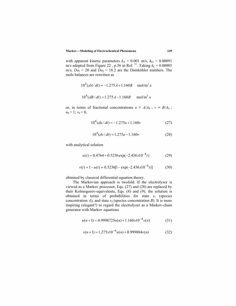
Markov—Modeling of Electrochemical Phenomena 149
with apparent kinetic parameters kf1 = 0.001 m/s, kb1 = 0.00091
m/s adopted from Figure 22 , p.56 in Ref. 31. Taking kL = 0.00005
m/s, Da1 = 20 and Da2 = 18.2 are the Damköhler numbers. The
mole balances are rewritten as
BAdtdA 160.1275.1)/(104 mol/m3.s
BAdtdB 160.1275.1)/(104 mol/m3.s
or, in terms of fractional concentrations u A/A0 ; v B/A0 ;
u0 = 1; v0 = 0,
vudtdu 160.1275.1)/(104 (27)
vudtdv 160.1275.1)/(104 (28)
with analytical solution
)10436.2exp(5236.04764.0)( 4txtu (29)
)]10436.2exp(1[5236.0)(1)( 4txtutv (30)
obtained by classical differential equation theory.
The Markovian approach is twofold. If the electrolyzer is
viewed as a Markov processor, Eqs. (27) and (28) are replaced by
their Kolmogorov-equivalents, Eqs. (8) and (9); the solution is
obtained in terms of probabilities for state s1 (species
concentration A), and state s2 (species concentration B). It is more
inspiring (elegant?) to regard the electrolyzer as a Markov-chain
generator with Markov equations
)(10160.1)(9998725.0)1( 4 nvxnunu (31)
)(999884.0)(10275.1)1( 4 nvnuxnv (32)
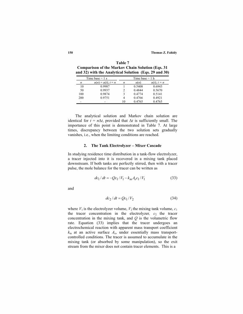
Thomas Z. Fahidy 150
Table 7
Comparison of the Markov Chain Solution (Eqs. 31
and 32) with the Analytical Solution (Eqs. 29 and 30)
Time base = 1 s Time base = 1 h
n u(n) = u(t); t = n n u(n) u(t); t = n
10 0.9987 1 0.5408 0.6943
50 0.9937 2 0.4844 0.5670
100 0.9874 3 0.4774 0.5141
200 0.9751 4 0.4766 0.4921
- - 10 0.4765 0.4765
The analytical solution and Markov chain solution are
identical for t = n t, provided that t is sufficiently small. The
importance of this point is demonstrated in Table 7. At large
times, discrepancy between the two solution sets gradually
vanishes, i.e., when the limiting conditions are reached.
2. The Tank Electrolyzer – Mixer Cascade
In studying residence time distribution in a tank-flow electrolyzer,
a tracer injected into it is recovered in a mixing tank placed
downstream. If both tanks are perfectly stirred, then with a tracer
pulse, the mole balance for the tracer can be written as
11111 /// VcAkVQcdtdc em (33)
and
212 // VQcdtdc (34)
where V1 is the electrolyzer volume, V2 the mixing tank volume, c1
the tracer concentration in the electrolyzer, c2 the tracer
concentration in the mixing tank, and Q is the volumetric flow
rate. Equation (33) implies that the tracer undergoes an
electrochemical reaction with apparent mass transport coefficient
km at an active surface Ae, under essentially mass transport-
controlled conditions. The tracer is assumed to accumulate in the
mixing tank (or absorbed by some manipulation), so the exit
stream from the mixer does not contain tracer elements. This is a

Markov—Modeling of Electrochemical Phenomena 151
Table 8
Comparison of the Markov Chain Solution (Eqs. 35
and 36) with the Analytical Solution (Eqs. 33 and 34).
Q/V = 2.5x10⁻³
min-1
; (Q + kmAe)/V = 3.5x10⁻³
min-1
;
Dimensionless Concentrations: c1(0) = 1; c2(0) = 0; t
= 0.1 min; t = 0.1n
Markov chain Analytical solutiona
n c1(n) 102 c2(n) c1(t) 102 c2(t)
1 0.99965 0.0250 0.99965 0.0250
2 0.99939 0.0500 0.99930 0.0500
5 0.99825 0.1249 0.99825 0.1249
10 0.99651 0.2500 0.99651 0.2495
50 0.98265 1.2390 0.98265 1.2390
100 0.96560 2.4570 0.96560 2.4560
200 0.93238 4.8300 0.93239 4.8280
500 0.89943 11.469 0.83946 11.466 a c1(t) = exp(–3.5x10⁻³t)
c2(t) = 0.7142exp[1 – exp(–3.5x10⁻³t)]
[t] : min
modification of the configuration discussed by Tamir1 (Section
4.3-1, pp. 353–355) via the inclusion of the electrochemical
process. Rewriting the mole balances as 1111 ;/ cdtdc
1/)( VAkQ em and 22122 /;/ VQcdtdc , the Markov
equations are obtained as
)()1()1( 111 nctnc (35)
)()()()1( 2122 ncnctnc (36)
If t = 1 in terms of a convenient time unit, c1(n+1) = (1 –
µ1)c1(n), and c2(n + 1) = µ2c1(n) + c2(n). The limiting conditions
yield c1* = 0 and c2
* = 1, if dimensionless concentrations are
employed, using e.g., the initial amount of tracer concentration as
reference. Table 8 indicates very good agreement up to large
times between the analytical and Markov chain solution, when the
size of t is judiciously chosen.

Thomas Z. Fahidy 152
3. Markovian Analysis of the CSTER23
In the Markovian view of the CSTER (continuous-flow stirred
tank electrochemical reactor) transitional probabilities related to
flow and reaction describe the history of an element (molecule,
ion, particle, etc.). A convenient framework for analysis considers
the interior of the reactor as state s1, and exit as s2, as an absorbing
state. Then, p11(n) denotes the probability that an element has not
undergone reaction, and is inside the reactor at stage n (i.e., time
instant n t). Consequently, p12(n) is the probability that the
element at stage n has left the reactor, while it had been in the
reactor at stage n – 1. The probability that at stage n the element
was in the reactor, while it had been in the exit stream at stage n-
1, is p21(n). Finally, p22(n) denotes the probability that an element
in the exit stream a stage n was in the exit stream at stage n – 1. In
the absence of backmixing or recycling, p21(n) = 0. In a perfectly
mixed reactor the transitional probability of outflow over a time
period t is Q t/V, if Q is the volumetric flow rate and V is the
active volume.
In this context, the mole balance for a reacting element (e.g.,
active ion):
VcAkVQcVQcdtdc emi //// 111(37)
may be rewritten as a Markov equation
)()1()1( 1111 ncpnxnc i (38)
where xi(n) = Q tci(n)/V represents the reacting element inflow
with inlet concentration ci(t), and p11 = 1 – [(Q + kmAe)/V] t. If the
inlet concentration remains constant, xi(n) = xi does not vary with
n.
The importance of choosing a suitably small t is again
shown in Table 9; if t is too large, the Markovian approach
yields a meaningless temporary rise in c1. Nonetheless, the
limiting value c1* = 9.663x10⁻³ mol dm-3 is predicted correctly.
In a more sophisticated version, the analysis is based on three
states. The transition probability p13 pertains to the bypass of an
element entering the reactor to the exit state without participating
in the electrode process. To analyze a CSTER with partial

Markov—Modeling of Electrochemical Phenomena 153
Table 9
Illustration of the Importance of
Suitably Small t Values for
Markovian Analysis of a CSTER.
Q = 2 dm3 min
-1;
ci = 0.01 mol dm-3
; V = 10 dm3;
Ae = 700 cm2; km = 10
-4cm s
-1;
c1(0) = 0.01 mol dm-3
; t = n t
t = 1 min t = 0.1 min
n c1(n) c2(n) c1(t) = c2(t)
0 10 10 10
1 12 9.94 9.99
2 11.52 9.88 9.99
3 29.13 9.84 9.98
4 25.10 9.81 9.97
5 21.91 9.78 9.97
All concentrations in mmol dm-3 units
c1* = 9.66
backmixing,a four-state model has been shown to be attractive
(Section 5, Ref. 23).
V. THE MARKOV–CHAIN APPROACH TO
MISCELLANEOUS ASPECTS OF ELECTROCHEMICAL
TECHNOLOGY
Markov theory can be applied advantageously to a variety of
technological problems of day-to-day operation in an industrial
environment. Such problems transcend the realm of purely
physico-chemical and fundamental electrochemical
considerations, and are closely linked to (large-scale)
technological aspects. This Section demonstrates the utility of the
Markovian approach to selected examples.
1. Repair of Failed Cells
An electrolytic cell bank producing a commercial product consists
of m number of cell units. Due to various reasons (e.g., imperfect

Thomas Z. Fahidy 154
control of electrolyte composition and/or purity), cells can be
short-circuited temporarily. It is assumed that the Poissonian
failure-density parameter is , i.e., that the probability of short-
circuiting of a cell during time interval t is t. The repair of
short-circuited cells requires time whose distribution is
exponential with density parameter µ.
In the simplest case (suppressing the trivial situation of no
repair being available), there is one repair station (mechanic,
technician, etc.) available at any given time. The task is to
determine the limiting probability distribution of j cells being out
of order, assuming time-independent conditions. The starting
point of this procedure is Eq. (13), stated again as
mjp ij
m
i
i ,...,0;0
0
* (13)
The slightly changed notation reflects the choice of states: s0 is the
state of normal operation, and state sj is the state of being out of
order due to short-circuiting of j number of cells. Thus, 00
represents normal operation, and 0j represents the breakdown of j
number of cells, etc. t is sufficiently small for only one cell to
become short-circuited, or repaired within this time interval. For
the j = 0 case, Eq. (13) expands to
010*100
*0 pp (39a)
and since 00 = –m , 10 = µ, it follows that
*1
*0 ppm (39b)
If m = 1, Eq. (13) yields p0*
01 + p1*
11 = 0. Since 01 = and 11 =
µ, p0* = µp1
*. This relationship can more simply be obtained by
setting m = 1 in Eq. (39b). If m = 2, Eq. (13) expands to:
j = 1: 021*211
*101
*0 ppp (40a)
j = 2: 022*212
*102
*0 ppp (40b)

Markov—Modeling of Electrochemical Phenomena 155
Since 01 = 2 ; 02 = 0; 11 = –( + µ); 12 = ; 21 = µ; 22 = –µ; the
final forms become
j = 1: *2
*0
*1 2)( ppp (41a)
j = 2: *2
*1 pp (41b)
Table 10 summarizes the reasoning behind the establishment
of the ij values. By successive development, the expansion set
j = 1: *2
*0
*1 3)2( ppp (42a)
j = 2: *3
*1
*2 2)( ppp (42b)
j = 3: *3
*2 pp (42c)
is obtained for the case of m = 3. In the general case, the limiting
probability distribution is given by the set of equations
*1
*0 ppm (43a)
*1
*1
* )1(])[( jjj ppjmpjm (43b)
Table 10
Development32
of the Transitional Probability Density
Parameters of Eq. (13); m = 2
Relationship Substantiation
01 = 2 Either one of the two cells can break down
02 = 0 Only one cell can break down within t
11 = –( + µ) No new breakdown; no new repair
12 = Second cell breaks down, first cell not repaired
21 = µ One cell repaired; one cell still out of order
22 = –µ Neither cell has been repaired

Thomas Z. Fahidy 156
*1
*mm pp (43c)
Equations (43) are also stated by Rozanov5 (p. 113, Problem 6)
without derivation.
The limiting probability of exactly j cells being out of order is
obtained by setting j = 0, 1,…, m in Eq. (43) and recalling that all
probabilities add up to unity, as5
mjpjmmp jj ,...,1,0;)/]()!/(1/[( *0pmnm (45)
A typical distribution is portrayed in Table 11 for a
configuration of fifty cells arranged in five ten-cell banks, where
for the sake of safety, a short-circuited cell will disconnect an
entire bank. This arrangement is essentially identical to a five-cell
bank with single short-circuits. The more efficient (i.e., the faster)
the repair service (i.e., the smaller /µ), the smaller the probability
that short-circuited cells are not repaired at any arbitrary time.
Conversely, if repair takes a long time, a certain number of cells
will always be short-circuited, and if /µ is extremely large, a
complete shutdown of cell operation will be highly probable (the
/µ = 10, p5* 0.9 case is a case in point, albeit not overly
realistic.)
Table 11
Limiting Probability Distribution for Exactly j = 0,1,…,5 Cells
being Short-Circuited, as a Function of Repair Efficiency /µpj
/µ j = 0 j = 1 j = 2 j = 3 j = 4 j = 5nm
0.1 0.564 0.282 0.113 0.034 6.8x10⁻³ 6.8x10⁻⁴ 0
0.5 0.0367 0.0917 0.183 0.275 0.275 0.138 2.11
1 3.7x10⁻³ 0.0153 0.0614 0.184 0.368 0.368 3.01
5 2.2x10⁻⁶ 5.46x10⁻⁵ 1.09x10⁻³ 0.0164 0.164 0.819 3.8
10 7.5x10⁻⁸ 3.77x10⁻⁷ 1.51x10⁻⁴ 4.53x10⁻³ 0.090 0.905 3.9

Markov—Modeling of Electrochemical Phenomena 157
2. Analysis of Switching–Circuit Operations
An electrolytic plant (e.g., a metal refinery) may operate m
number of cells which have to be taken out of service temporarily
at regular time intervals. The probability that a cell is being put
back into service within a small t time period is t, where is
the density parameter. The probability that a cell is taken out of
operation within t is µ t, and µ is the second density parameter.
The limiting probabilities pj* ; j = 0,1,2…,m of exactly j number of
cells being switched back into operation can be obtained by a
procedure identical to the electrical power line/machine operation
problem stated by Rozanov5 (Problem 9, p. 114) and Sveshnikov6
(Problem 39.16, pp. 255–256; 455):
*1
*0 ppm (46a)
*1
*1
* )1()(])[( jjj pjpjmpjjm (46b)
*1
*mm ppm (46c)
whose derivation is similar to the one in Section V.1 . Systematic
iteration yields
mj
jmjmp jjmj
,...,2,1,0 ;
)]/([)]/(][)!(!/[(!*
(47)
Table 12 illustrates the computation procedure in the case of
m = 5; the plant may be envisaged, as in Section V.1, to consist of
m cell banks, the quantity j denoting the number of banks
switched back into operation. In the specific case of = µ (equi -
probability of switching into either direction), Eq. (47) reduces to
the binomial probability distribution of selecting j elements out of
m identical elements with a single-event probability of ½.
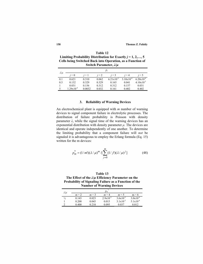
Thomas Z. Fahidy 158
Table 12
Limiting Probability Distribution for Exactly j = 1, 2,…, 5
Cells being Switched Back into Operation, as a Function of
Switch Parameter, /µ
pj
/µj = 0 j = 1 j = 2 j = 3 j = 4 j = 5
0.1 0.621 0.310 0.062 6.21x10⁻³ 3.10x10⁻⁴ 6.20x10⁻⁶
0.5 0.132 0.329 0.329 0.165 0.041 4.10x10⁻³
1 0.031 0.156 0.312 0.312 0.157 0.031
5 1.29x10⁻⁴ 0.0032 0.032 0.161 0.402 0.402
3. Reliability of Warning Devices
An electrochemical plant is equipped with m number of warning
devices to signal component failure in electrolytic processes. The
distribution of failure probability is Poisson with density
parameter , while the signal time of the warning devices has an
exponential distribution with density parameter µ. The devices are
identical and operate independently of one another. To determine
the limiting probability that a component failure will not be
signaled it is advantageous to employ the Erlang formula (Eq. 15)
written for the m devices:
m
j
jmm jmp
0
* ])/)(!/1(/[)/)(!/1( (48)
Table 13
The Effect of the /µ Efficiency Parameter on the
Probability of Signaling Failure as a Function of the
Number of Warning Devices
pm*
/µm = 2 m = 3 m = 4 m = 5 m = 6
½ 0.143 0.023 2.9x10⁻³ 3.6x10⁻⁵ 3.0x10⁻⁶
1 0.200 0.045 0.015 3.1x10⁻³ 5.1x10⁻⁴
2 0.400 0.210 0.095 0.037 0.012

Markov—Modeling of Electrochemical Phenomena 159
to ascertain the number of warning devices needed in order to
ensure that the probability of failure-signaling does not exceed a
predetermined value. As shown in Table 13, pm* is highly
sensitive to the device efficiency ( /µ).
4.
Electrolyzer
In a complex reaction system occurring in a flow electrolyzer, one
of the anode reaction products reacts with the principal constituent
of the composite electrolyte, yielding an anionic species whose
parasitic reaction at the cathode reduces the cathode efficiency.
Due to system complexity and paucity of information about the
reaction mechanism(s), a Markov process model is proposed with
probability pk = k exp(– )/k! of the production of k ions of the
anionic species; is the mean of the postulated Poisson
distribution. The model also stipulates a probability q of reaction
of the anionic species during two successive equal time periods of
t each.
The limiting probabilities pj* for the number of ionic species
in the system can be established in a manner similar to the
production/decomposition of a radioactive particle possessing the
same probabilistic properties6 (Example 38.3, pp. 237–238). The
result of an involved algebraic manipulation, itself a Poisson
distribution:
,...1,0;/);exp()!/(* jqjp jj (49)
is not explicitly dependent on k. As indicated previously, the
number of ionic species can conveniently be interpreted to mean a
cluster of ions, whose (arbitrary) size depends on the properties of
the electrochemical system examined. Table 14 depicts the rapid
increase in the number of (unreacted) anions with an increase in µ.
When, e.g., µ = 10, p9* = p10
* = 0.125 is the largest individual
probability, but the descent of pj* from the maximum value is slow
[p*(15) = 0.035; p(20)* = 0.0019; p(25)* = 2.9x10⁻⁵.] Cumulative
probabilities are expectably higher, e.g., the probability that, when
Monitoring of Parasitic Reaction Sequence in an

Thomas Z. Fahidy 160
Table 14
Limiting Probability Distribution for Exactly j = 0, 1, 2,…
Number of an Ionic Species Existing in the Electrolyte, as a
Function of the /q Ratio in Eq. (49)
pj*
µ/j = 0 j = 1 j = 2 j = 3 j = 4 j = 5 j = 6
0.1 0.905 0.091 4.5x10⁻³ 2.0x10⁻⁴ 3.8x10⁻⁶ 7.5x10⁻⁸ 2.5x10⁻¹⁷
0.5 0.607 0.303 0.076 0.013 1.6x10⁻³ 2.0x10⁻⁴ 1.6x10⁻¹⁰
1.0 0.368 0.368 0.184 0.061 0.015 3.1x10⁻³ 1.0x10⁻⁷
5.0 6.7x10⁻³ 0.034 0.084 0.140 0.176 0.176 0.018
10.0 4.5x10⁻⁵ 4.5x10⁻⁴ 2.3x10⁻³ 7.6x10⁻³ 0.019 0.038 0.125
µ = 0.1, not more than three anions/anion clusters are present is
virtually 100%.
5. Flow Circulation in an Electrolytic Cell
The interaction of forced and natural convective flow between
cathodes and anodes may produce unusual circulation patterns
whose description via deterministic flow equations may prove to
be rather unwieldy, if possible at all. The Markovian approach
would approximate the true flow pattern by subdividing the flow
volume into several zones, and characterize flow in terms of
transition probabilities from one zone to others. Under steady
operating conditions, they are independent of stage n, and the
evolution pattern is determined by the initial probability
distribution. In a similar fashion, the travel of solid pieces of
impurity in the cell can be monitored, provided that the size,
shape and density of the solids allow the pieces to be swept freely
by electrolyte flow.
Table 15 illustrates the development of the probability
distribution of a solid particle being in one of the three
characteristic zones in a cell, assuming that the particle residence
has an equiprobable initial state, and that the transitional
probabilities are as follows. Zone 1 2:0.4; Zone 2 1:0.4; Zone
1 3: 0.1;Zone 3 1:0.2; Zone 2 3:0.3; Zone 3 2:0.2 .
The continuous circulation of flow elements inside the
electrolyzer is due to the donor-acceptor nature of each zone. If,
however, at least one of the zones is an absorbing Markov state,

Markov—Modeling of Electrochemical Phenomena 161
Table 15
Probability Distribution of a
Solid Particle being in One
of Three Flow Circulation
Zones with an Equiprobable
Initial-State Probability.
p11 = 0.5; p12 = 0.4; p13 = 0.2;
p21 = 0.4; p22 = 0.3; p23 = 0.6;
p31 = 0.1; p32 = 0.3; p33 = 0.2
n p1(n) p2(n) p3(n)
0 1/3 1/3 1/3
1 0.367 0.433 0.200
2 0.397 0.397 0.206
3 0.398 0.402 0.200
4 0.400 0.400 0.200
0.400 0.400 0.200
the distribution pattern eventually excludes all states except the
absorbing state(s). If the exit zone is the only absorbing state, the
probability that flow elements/solid particles will eventually flow
out of the electrolyzer is 100%. Tables 16 and 17 indicate the
slow rate whereby the limiting probabilities are reached. The
initial state probability distribution is immaterial, since the
eigenvector associated with eigenvalue of unity (Section II.1) has
one element of unity, irrespective of the pij values (Appendix),
while the other elements are zero.
VI. FINAL REMARKS
Unidirectional kinetic processes cannot be immediately
interpreted as Markov chains, since only the (1,1) element of the
P-matrix would differ from zero, violating the stochastic matrix
constraints (Section II.1). An artificial Markov matrix complying
with this constraint can be visualized, however, with the
understanding that no other element of this imbedded P-matrix,
past the (1,1) element, will have a physical meaning. It follows
that the initial state probability vector is non-zero only in its (1,1)

Thomas Z. Fahidy 162
Table 16
Probability Distribution of a Solid
Particle being in One of Three Flow
Circulation Zones with an Initial
Distribution of p10= 1; p2
0= 0;
p30= 0. The Transition Probabilities
are: Zone 1 2: 0.2; Zone 1 3: 0.1;
Zone 2 3: 0.05
n p1(n) p2(n) p3(n)
0 0.700 0.200 0.100 1 0.700 0.200 0.100
5 0.168 0.485 0.347
10 0.028 0.456 0.515
20 8.0x10⁻⁴ 0.286 0.713
30 2.2x10⁻⁵ 0.172 0.828
50 1.8x10⁻⁸ 0.062 0.938
100 3.2x10⁻¹⁶ 0.005 0.995
150 5.8x10⁻²⁴ 3.6x10⁻²⁴ 0.9996
element, and that it has to be unity. The small-signal analysis36
and large-step coulostatic analysis37 employed in electroanalytical
chemistry provide a good case in point.
The variation of overpotential with time is given by the
expression
Table 17
Probability Distribution in Table 16
Modified by Additional Transitional
Probability for Zone 2 1: 0.1
n p1(n) p2(n) p3(n)
0 0.700 0.200 0.100
1 0.700 0.200 0.100
5 0.255 0.392 0.353
10 0.141 0.314 0.545
20 0.069 0.163 0.768
30 0.035 0.083 0.881
50 0.009 0.022 0.969
100 3.23x10⁻⁴ 7.59x10⁻⁴ 0.999
150 1.13x10⁻⁵ 2.65x10⁻⁵ 0.99996
0 0 1

Markov—Modeling of Electrochemical Phenomena 163
0)0(;)/1(/ tdtd c (50)
where the time constant c = RTCd/nFi0 is a lumped parameter
incorporating the surface capacity Cd, and exchange current
density i0. The Markovian approach assigns an imbedded
transition probability matrix with elements p11 = 1 – t/ c , p12 = 0;
p21 = t/ c , p22 = 1, and the initial state probability vector has
elements p10 = 1; p2
0 = 0. Consequently, the stage-dependent
elements are p11(n) = (1 – t/ c)n , and p12 (n) = 1 – (1 – t/ c)
n , the
latter being irrelevant. Comparison with the analytical solution of
Eq. (50) in Table 18 indicates, as expected, that close agreement
can be attained if t is sufficiently small.
It is instructive to note that the standard first-order forward
difference discretization of Eq. (50) is finite difference calculus:
ttttdtd /)]()([/ (51)
also leads to the Markov chain solution in the second column of
Table 18.
Table 18
Comparison of the Analytical Solution of Eq.
(50) and the Markov Chain Solution.
T = 293 K; Cd = 2x10⁻⁵
F cm-2
; i0 = 10-5
A cm-2
;
n = 2; R = 8.3143 J mol-1
K-1
;
F = 96488 C mol-1
; t = 0.1 ms; c = 25.25 ms
n Markov chain:
Y(n) = (0.99604)nAnalytical solution:a
Y(0.1n) = exp(–0.00396n)
0 1 1
1 0.99604 0.99605
2 0.99210 0.99211
3 0.98817 0.98819
4 0.98425 0.98428
5 0.98036 0.98039
10 0.96110 0.96117
50 0.82005 0.82037
100 0.67248 0.67301
1000 0.01891 0.01906 a Y = / (0)
Thomas Z. Fahidy 164
At this time, it would be hazardous to predict the eventual
extent of influence Markov theory will attain in the realm of
electrochemistry and electrochemical engineering. Much terrain
remains to be explored, especially in the potential of
multidimensional chains and processes. If this chapter succeeds in
kindling at least some sustained interest in the subject matter, it
will have reached its ultimate objective.
ACKNOWLEDGMENTS
Author’s work in various domains of probability theory applied to electrochemical phenomena has been supported by the Natural
Sciences and Engineering Research Council of Canada (NSERC),
and the University of Waterloo.
APPENDIX
Eigenvalues and Eigenvectors of the Transition Probability
Matrix
Under limiting conditions, the state probabilities become
invariant, i.e., past a sufficiently large value n > N, p(n + 1) =
p(n); n = N, N + 1; N + 2,…, hence p(n) = Pp(n). Invoking the
classical eigenvalue theorem of matrix algebra e = Pe for the
Markov matrix P results in the important finding that that the
limiting probabilities are elements of the eigenvector e pertaining
to the specific eigenvalue = 1. However, the unity eigenvalue is
not the only one, because the total number of eigenvalues equals
the number of states. The = 1 is, however, the only admissible
eigenvalue of P.
As an illustration, the oscillatory behaviour of anodic copper
dissolution discussed in Section III.3, with P elements shown in
Table 5, is chosen. The eigenvalue theorem yields three
relationships (k = 1,2,3):
kkkkk eeee 1321 4.05.01.0 (52)

Markov—Modeling of Electrochemical Phenomena 165
kkkk eee 221 1.08.0 (53)
kkkkk eeee 3321 6.04.01.0 (54)
To find pk*, k = 1,2,3 = 1 is set and the solution of the above
equations yields p1* = 36/109 0.3303; p2
* = 32/109 0.2936;
p3* = 41/109 0.3761.
The eigenvalues are given by the characteristic equation of
the P matrix:
011.031.08.0 23 (55)
as 1 = 1; 2 0.0567 and 3 –0.3285. The eigenvectors for the
second and third eigenvalues are, respectively: –0.2311; 4.2695;
–3.1008, and –5.7669; 10.784; –4.0172. Since probabilities
cannot be negative, and cannot be larger than unity, these
eigenvector elements cannot be interpreted as probabilities. The
limiting probabilities are the elements of the first eigenvector
36/109; 32/109; 41/109.
The eigenvalue theorem, a standard topic in any linear
algebra text and mathematics book, is particularly well presented
by Dixon,33 Wilf,34 and Nicholson.35
REFERENCES
1A. Tamir, Application of Markov Chains in Chemical Engineering, Elsevier,
Amsterdam, 1998. 2V. S. Pugachev, Teoriya Sluchainikh Funktzii (Theory of Random Functions),
Gos. Izd. Fiziko-Matem. Liter., 2nd Ed.., Moscow, 1960, Section 46, pp. 191–202. 3E. Parzen, Modern Probability Theory and Its Applications, Wiley and Sons,
New York, 1960, Chapter 3, Section 3, pp. 136–147. 4H. Stark and J. W. Woods, Probability, Random Processes and Estimation
Theory for Engineers, Prentice Hall, Englewood Cliffs, 1986. 5Y. A. Rozanov, Probability Theory: A Concise Course, Dover, New York, 1969,
Chapter 7, pp. 83–101; Chapter 8, pp.102 – 114. 6A. A. Sveshnikov, Problems in Probability Theory, Mathematical Statistics and
Theory of Random Functions, Dover, 1968, Chapter VIII, pp. 231–274. 7F. R. Gantmacher, The Theory of Matrices, Chelsea Publishing, New York, 1959,
Vol. 2, Chapter XIII, Sections 6 – 8, pp. 80 – 98. 8M . D. Greenberg, Advanced Engineering Mathematics, 2nd Ed., Prentice Hall,
Upper Saddle River, 1998, Section 11.2, pp. 546 – 549.
Thomas Z. Fahidy 166
9W. J. Stewart, Introduction to the Numerical Solution of Markov Chains,
Princeton Univ. Press, 1994. 10A. Sinclair, Algorithms for Random Generation and Counting: a Markov Chain
Approach, Birehäuser, Boston, 1993. 11W. J. Anderson, Continuous-Time Markov Chains: An Applications-Oriented
Approach, Springer–Verlag, New York, 1991.12O. Hernandez-Lerma, Adaptive Markov Control Processes, Springer-Verlag,
New York, 1989.13G. Winkler, Image Analysis, Random Fields and Markov Chain Monte Carlo
Methods, Springer-Verlag, New York, 2003. 14P. Baldi, L. Mazliak, and P. Priouret, Martingales and Markov Chains, Chapman
and Hall/CRC, Boca Raton, 2002. 15T. Z. Fahidy, Can. J. Chem. Eng. 65 (1987) 1009. 16G. Radons, J. D. Becker, B. Duelfer, and J. Krueger, Biol. Cybern. 71 (1994)
359.17A. Opri an, S.-A. Opri an, and M. Ignat, Analele Stiin ifice Ale Universit tii
“Al.I. Guza”, (in English), Iasi (Romania), 1997 – 1998. 18S. A. Godorr, B. D. Young and A. W. Bryson, Chem. Eng. Commun. 117 (1992)
307.19T. Witten and L. M. Sauder, Phys. Rev. Lett. 47 (1981) 1400. 20T. Witten, and L. M. Sauder, Phys. Rev. B 27 (1983) 5686. 21F. Argoul, A. Arneodo, G. Grasseau, and H. L. Swinney, Phys. Rev. Lett. 61
(1988) 2558. 22M. R. Dudek, W. M. Trochimczuk, and R. Wycizk, J. Membrane Sci. 67 (1992)
273.23T. Z. Fahidy, J. Appl. Electrochem. 17 (1987) 841. 24L. J. Goldstein, and D. I. Schneider, Finite Mathematics and Its Applications, 2nd
Ed., Prentice Hall, Englewood Cliffs, 1984, Chapter 8, pp. 329 – 360. 25T. Z. Fahidy, Chem. Eng. Edu. 27 (1993) 42. 26D. C. Montgomery, G. C. Runger, and N. F. Hubele, Engineering Statistics, 2nd
Ed., Wiley and Sons, New York, 2001, Section 2.1, Exercise 2.3, p. 25. 27Z. H. Gu, J. Chen, and T. Z. Fahidy,Electrochim. Acta 37 (1992) 2637. 28T. Z. Fahidy, J. Appl. Electrochem. 28 (1998) 411. 29J. O’M. Bockris, A. K. N. Reddy, and M. Gamboa-Aldeco, Modern
Electrochemistry, 2nd Ed., Plenum, New York, Volume 2A: Fundamentals of
Electrodics, Section 6.2.6.2, p. 804. 30L. H. Van Vleck, Elements of Materials Science and Engineering, 4th Ed.,
Addison-Wesley, Reading, Mass., 1980, Appendix B, pp. 520 -523. 31K. Scott, Electrochemical Reaction Engineering, Acad. Press, London, 1991,
Section 2.1.2, pp. 52 – 56. 32T. Z. Fahidy, unpublished results 33C. Dixon, Linear Algebra, Van Nostrand Reinhold, New York, 1971, Section
VII.1, pp. 135 – 140. 34H. S. Wilf, Mathematics for the Physical Sciences, Dover, New York, 1962,
Section 1,12, pp. 18 – 20. 35W. K. Nicholson, Elementary Linear Algebra With Applications, Prindle, Weber
and Smith, Boston, 1986, Section 7.1, pp. 311 – 324 36A. J. Bard, and L. R. Faulkner, Electrochemical Methods, Wiley and Sons, New
York, 1980, Section 7.7.2, pp. 273 – 274. 37Idem, ibid. Section 7.7.3, pp. 275 – 276.

167
4
Fractal Approach to Rough Surfaces and
Interfaces in Electrochemistry
Joo-Young Go and Su-Il Pyun*
Department of Materials Science and Engineering, Korea Advanced Institute of
Science and Technology, 373-1, Guseong-dong, Yuseong-gu, Daejeon, 305-701,
Republic of Korea*Corresponding author; Tel.: +82-42-869-3319; Fax: +82-42-869-3310;
E-mail: [email protected]
I. INTRODUCTION
The real objects found in nature have complex structures whichEuclidean geometry can not characterize. After Mandelbrot1
developed a new geometry, i.e., fractal geometry, which providesa new paradigm for understanding many physical phenomena innature, fractal geometry has been widely used in a number offields, e.g., science, art,2-4 economics,5-8 etc. Especially, in science,the characterization of the rough surfaces and interfaces usingfractal geometry has played an important role in understanding theanomalous behavior of rough surfaces and interfaces.
There are three kinds of fractals as shown in Figure 1.9-11 Thefirst one is a surface fractal, i.e., a dense object with a fractal
Modern Aspects of Electrochemistry, Number 39, edited by C. Vayenas et al.,Springer, New York, 2005.

Figu
re 1
. S
chem
atic
dia
gram
s of
thre
e ki
nds
of f
ract
als.
(a)
A s
urfa
ce f
ract
al, (
b) a
mas
s fr
acta
l, an
d (c
) a
pore
fra
ctal
.
Joo–Young Go and Su-Il Pyun168
(a)
(b)
(c)

Fractal Approach to Rough Surfaces and Interfaces 169
surface (Figure 1a). The second one is a mass fractal, i.e., a fractalobject such as a network or cluster, whose surface is also fractal(Figure 1b). Finally, the last one is a pore fractal, i.e., a denseobject in which there exists a distribution of holes or pores with afractal structure (Figure 1c). Since it is one of the most interestingissues to estimate accurately real active area in an electrochemicalsystem, many researchers have given a lot of attention to surfacefractal as a powerful tool to quantify the geometrical irregularityof the electrode surfaces and various interfaces. In this respect, wefocus on surface fractal rather than mass and pore fractals in thisarticle.
Diffusion-limited electrochemical techniques as well asphysical techniques have been effectively used to determine thesurface fractal dimensions of the rough surfaces and interfacesmade by electrodeposition,12-26 fracture,27-32 vapor deposition,21,33-
46 corrosion,47-54 surface modification such as machining andplasma irradiation,55-60 etc. Many rough surfaces and interfaces areself-similar fractals which show isotropic scaling behavior in alldirections, but most rough surfaces and interfaces are morecomplex self-affine fractals which show asymmetric scalingbehavior perpendicular to the surface.
Since self-similar and self-affine fractals show differentscaling properties, the surface fractal dimension of the roughsurfaces and interfaces must be determined based on their inherentscaling properties. However, a little attention has been paid toclarify whether the rough surfaces and interfaces show self-similarscaling property or self-affine scaling property and whether thephysical and electrochemical methods for the determination of thesurface fractal dimension are adequately used or not. In thisrespect, we review fractal approaches to rough surfaces andinterfaces in electrochemistry to give clear guidelines for theircharacterization using the surface fractal dimension.
The structure of this review is composed of as follows: inSection II, the scaling properties and the dimensions of self-similar and self-affine fractals are briefly summarized. Thephysical and electrochemical methods required for thedetermination of the surface fractal dimension of rough surfacesand interfaces are introduced and we discuss the kind of scalingproperty the resulting fractal dimension represents in Section III.

Joo–Young Go and Su-Il Pyun170
In Section IV, from the studies on diffusion towards self-affinefractal interface, the surface fractal dimension as determined bythe electrochemical method is characterized as being self-similar,even though the rough surfaces and interfaces show the self-affinescaling property. Finally, in Section V, we exemplified theapplication of fractal geometry in electrochemical systems in viewof the characterization of rough surfaces and interfaces by thesurface fractal dimension.
II. OVERVIEW OF FRACTAL GEOMETRY
The word ‘fractal’ was coined by Mandelbrot in his fundamentalbook.1 It is from the Latin adjective fractus which means broken
and it is used to describe objects that are too irregular to fit into atraditional geometrical setting. The most representative propertyof fractal is its invariant shape under self-similar or self-affinescaling. In other words, fractal is a shape made of parts similar tothe whole in some way.61 If the objects are invariant underisotropic scale transformations, they are self-similar fractals. Incontrast, the real objects in nature are generally invariant underanisotropic transformations. In this case, they are self-affinefractals. Self-affine fractals have a broader sense than self-similarfractals. The distinction between the self-similarity and the self-affinity is important to characterize the real surface in terms of thesurface fractal dimension.
From another point of view, fractals fall naturally into twocategories, i.e., nonrandom and random.1,62-64 When the enlargedpart overlaps the original object exactly, we call this object anonrandom fractal, viz., deterministic fractal. For example, thevon Koch curve, the Cantor set, the Sierpinski gasket, etc. whichare generated by iterative operation according to a growth rulebelong to nonrandom fractals. Their self-similar or self-affinescaling property is satisfied over all range of length scales.
However, nonrandom fractals are not found in nature. Manyobjects existing in nature belong to random fractal, viz., statisticalfractal, when the enlarged part is similar to the original object in astatistical sense. In practice, it is impossible to verify that allmoments of the distributions are identical, and claims of statistical
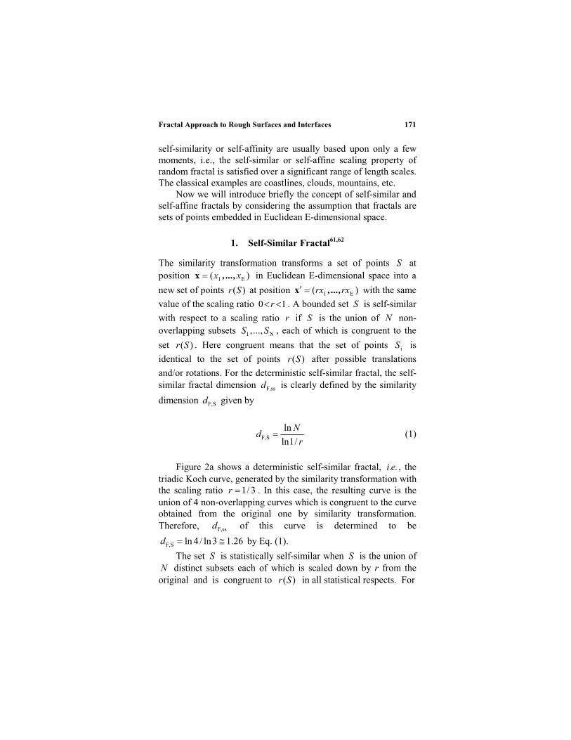
Fractal Approach to Rough Surfaces and Interfaces 171
self-similarity or self-affinity are usually based upon only a fewmoments, i.e., the self-similar or self-affine scaling property ofrandom fractal is satisfied over a significant range of length scales.The classical examples are coastlines, clouds, mountains, etc.
Now we will introduce briefly the concept of self-similar andself-affine fractals by considering the assumption that fractals aresets of points embedded in Euclidean E-dimensional space.
1. Self-Similar Fractal61,62
The similarity transformation transforms a set of points S atposition )( E1 xx ...,,x in Euclidean E-dimensional space into a
new set of points )(Sr at position )( E1 rxrx ...,,x with the same
value of the scaling ratio 10 r . A bounded set S is self-similar
with respect to a scaling ratio r if S is the union of N non-overlapping subsets N1 ...,, SS , each of which is congruent to the
set )(Sr . Here congruent means that the set of points iS is
identical to the set of points )(Sr after possible translations
and/or rotations. For the deterministic self-similar fractal, the self-similar fractal dimension ssF,d is clearly defined by the similarity
dimension SF,d given by
r
Nd
/1ln
lnSF, (1)
Figure 2a shows a deterministic self-similar fractal, ..ei , thetriadic Koch curve, generated by the similarity transformation withthe scaling ratio 3/1r . In this case, the resulting curve is theunion of 4 non-overlapping curves which is congruent to the curveobtained from the original one by similarity transformation.Therefore, ssF,d of this curve is determined to be
26.13ln/4lnSF,d by Eq. (1).
The set S is statistically self-similar when S is the union ofN distinct subsets each of which is scaled down by r from theoriginal and is congruent to )(Sr in all statistical respects. For
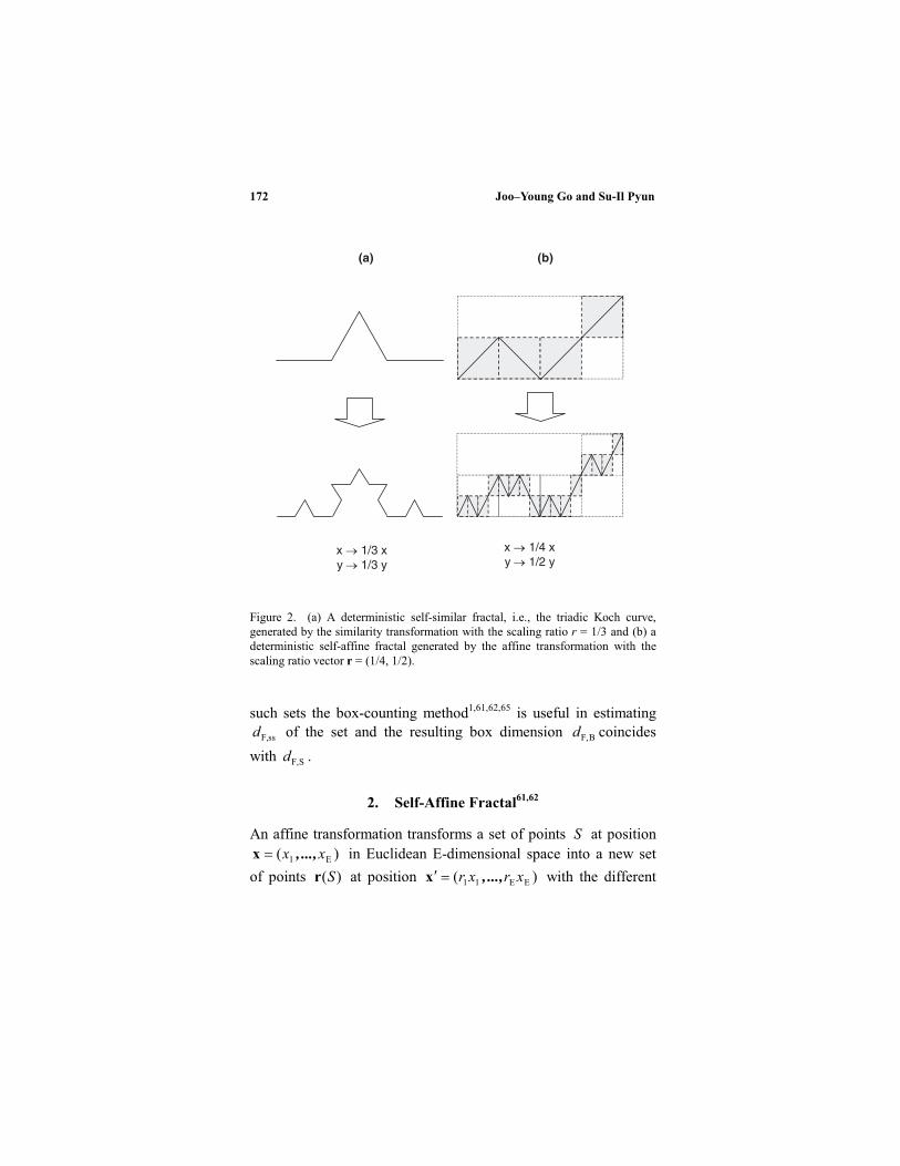
Joo–Young Go and Su-Il Pyun172
Figure 2. (a) A deterministic self-similar fractal, i.e., the triadic Koch curve,generated by the similarity transformation with the scaling ratio r = 1/3 and (b) adeterministic self-affine fractal generated by the affine transformation with thescaling ratio vector r = (1/4, 1/2).
such sets the box-counting method1,61,62,65 is useful in estimating
ssF,d of the set and the resulting box dimension BF,d coincides
with SF,d .
2. Self-Affine Fractal61,62
An affine transformation transforms a set of points S at position)( E1 xx ...,,x in Euclidean E-dimensional space into a new set
of points )(Sr at position )( EE11 xrxr ...,,x with the different
(a) (b)
x 1/4 xy 1/2 y
x 1/3 xy 1/3 y

Fractal Approach to Rough Surfaces and Interfaces 173
scaling ratios 1...,,0 E1 rr . A bounded set S is self-affine with
respect to a scaling ratio vector )...,,( E1 rrr if S is the union of
N non-overlapping subsets N1 ...,, SS , each of which is congruent
to the set )(Sr . Figure 2b shows a deterministic self-affine fractal
generated by the affine transformation with the scaling ratio vector1/2)(1/4,r . In this case, the resulting curve is the union of 4
non-overlapping curves which are congruent to the curve obtainedfrom the original one by the affine transformation.
In a similar way, the set S is statistically self-affine when S isthe union of N non-overlapping subsets each of which is scaleddown by r from the original and is congruent to )(Sr in all
statistical respects.In contrast to the self-similar case, the self-affine fractal
dimension saF,d of even the simplest self-affine fractal is not
uniquely defined.61,62,66 The similarity dimension SF,d exists only
for the self-similar fractal. For the self-affine fractal, there are twodifferent dimensions, i.e., a global dimension and a localdimension.11,61,62,65-67 The global dimension, which is observedabove a certain crossover scale, is simply 1Ed . Here, Ed
represents the topological dimension of the Euclidean space wherethe set is embedded. This means that, at large size level, the self-affine fractal looks essentially smooth.
It is the local dimension that describes the irregularity of theself-affine fractal. The local dimension can be determined by suchmethods as the box-counting method1,61,62,65 and the divider-walking method.61,66 The box dimension BF,d is defined by the
Hurst exponent H according to following equation
Hdd EBF, 10 H (2)
and the divider dimension DF,d is given by
Hd
1DF, 10 H (3)

Joo–Young Go and Su-Il Pyun174
where H represents the Hurst exponent which is a powerexponent observed in the power law between the root mean square(rms) roughness rms and the horizontal length L of the self-
affine fractal. From Eqs. (2) and (3), it is noted that BF,d and DF,d
do not coincide in value for the self-affine fractal. Therefore, theHurst exponent H uniquely characterizes the self-affine fractal.
III. CHARACTERIZATION OF ROUGH SURFACES AND
INTERFACES BASED UPON FRACTAL GEOMETRY:
METHODS NEEDED FOR THE DETERMINATION OF
THE SURFACE FRACTAL DIMENSION
1. Physical Methods
(i) Image Analysis Methods
The surface roughness is fundamental for several physicalproperties and physical phenomena on solid surfaces andinterfaces. In order to quantify the surface roughness, the solidsurfaces and interfaces are investigated using surface profiler orimaging equipments such as scanning electron microscope (SEM),transmission electron microscope (TEM) and scanning probemicroscope (SPM). And then the statistical roughness parametersare determined from the digitized surface profile or image. Thebest known roughness parameter is the root mean squareroughness (rms roughness) rms , but this parameter is rather
inadequate to provide a complete description of three-dimensionalsurface since it describes only vertical amplitude in a certainlateral direction.
Surface fractal dimension is an adequate roughness parametersince it represents both the vertical and the lateral information ofthree-dimensional surfaces over a significant range of lengthscales. In fractal analysis of the three-dimensional digitized imageof the surface morphology, SPM is a more adequate techniquethan SEM and TEM because of its high three-dimensionalresolution and nondestructive character. For example, by using ascanning tunneling microscope (STM) and an atomic force
Fractal Approach to Rough Surfaces and Interfaces 175
microscope (AFM), the surface morphology is directly describedby the digitized height data with a resolution down to the atomicscale, whereas using SEM and TEM, the two-dimensional cross-section of the surface morphology can be described by binarydigits.
Several algorithms have been used to determine surfacefractal dimension from SPM images. The most popular ones arethe power-spectrum method,1,2,68-71 the triangulation method,10,37,
43,45,61,66,72-75 the perimeter-area method,18-21,23,25,27,61,62,71,76-78 thestructure function method,2,56,57,70,76,79,80 the variance method,56,57
and the box-counting method.1,61,62,65,81,82 Among these algorithms,the triangulation method and the perimeter-area method areintroduced in this article as useful and reliable tools to determinethe self-similar and the self-affine fractal dimensions, respectively.
(a) Triangulation method10,37,43,45,61,66,72-75
In order to characterize the three-dimensional self-similarfractal surface, the self-similar fractal dimension ssF,d has been
determined from the analysis of the three-dimensional digitizedSPM image by using the triangulation method. This method isexactly analogous to the Richardson method1 for a profile.
Figure 3 describes schematically the algorithm used fordetermination of ssF,d by the triangulation method. The square
(x,y) plane with a cell size 2L is first divided into 2N equalsquares. This defines the location of the vertices of a number of
triangles. Then the electrode surface is covered by 22N trianglesinclined at various angles with respect to the (x,y) plane. These
22N triangles have equal projected triangle size TS (= NL / ),although their real areas are different.
The scaled surface area SSA, i.e., the measured surface area
by 22N triangles, is estimated to be the sum of the areas of all the22N triangles. This measurement is iterated as decreasing
projected triangle size TS, until every pixel in the AFM image
serves as the vertices of the 22N triangles. Then, ssF,d of the
surface is given by

Joo–Young Go and Su-Il Pyun176
Figure 3. Process of determination of the self-similar fractaldimension of the three-dimensional surface by the triangulationmethod.

Fractal Approach to Rough Surfaces and Interfaces 177
Figure 4. Dependence of the scaled surface area SSA on the projected trianglesize TS on a logarithmic scale obtained from the three-dimensional AFM image ofthe hot-rolled carbon steel surface. Here, s means TSlnd/SSAlnd .
2TSlogd
SSAlogdssF,d (4)
After measuring SSAs for the various projected TSs, theresulting SSAs are plotted as a function of the projected TS on alogarithmic scale. Figure 4 gives dependence of the scaled surfacearea SSA on the projected triangle size TS on a logarithmic scaleobtained from the three-dimensional AFM image of the hot-rolledcarbon steel surface. From the linear relationship between thelogarithm of SSA and the logarithm of projected TS, ssF,d of the
surface is determined using Eq. (4). In addition, it is possible todefine a length-scale range where the rough surface shows the
10-1 100 101 102
outer cutoff 0
103.33
103.31
103.29
103.27
103.25
dF,ss
= - (d log SSA / d log TS) + 2= - s + 2
s
Sca
led
Sur
face
Are
a S
SA
/ m
2
Triangle Size TS / m
Joo–Young Go and Su-Il Pyun178
fractal behavior by determining the inner and outer cutoffs inFigure 4. In the case of Figure 4, the spatial outer (upper) cutoff
o can be evaluated to be the value of TS where the linear line
with the slope of s and the horizontal line intersect. However, thespatial inner (lower) cutoff i can not be evaluated due to the
limitation in the resolution of the equipment, e.g., AFM.
(b) Perimeter-area method18-21,23,25,27,61,62,71,76-78
In order to characterize the self-affine fractal surface, the self-affine fractal dimension saF,d has been determined by using the
perimeter-area method. This method is based on the fact that theintersection of a plane with a self-affine fractal surface generatesself-similar lakes. This method is available for the imagesobtained by using SEM and TEM as well as SPM because it isused to analyze the two-dimensional digitized cross-section of thesurface. It is well known61,76 that the area A and the perimeter P
of the self-similar lakes are related to their fractal dimension LssF,d
by
2LssF,
LssF, /d
AdP (5)
where is a proportionality constant. The self-affine fractal
dimension of the original surface saF,d is related to LssF,d by
1LssF,saF, dd (6)
The algorithm used for determination of the self-affine fractaldimension by the perimeter-area method is given as follows:43,45,77
The three-dimensional digitized image of the surfacemorphology is cross-sectioned by a plane and then P and A ofthe resulting lakes are calculated. For instance, Figure 5a and 5bdepict the three-dimensional AFM image of the hot-rolled carbonsteel surface filled with water (black pixels) up to a heightcorresponding to 40 % of the maximum height of the surface andthe corresponding two-dimensional description of P (gray pixels)

Fractal Approach to Rough Surfaces and Interfaces 179
Figure 5. (a) Three-dimensional AFM image of the hot-rolledcarbon steel surface filled with water (black pixels) up to a heightcorresponding to 40% of the maximum height and (b)corresponding two-dimensional description of the perimeters(gray pixels) and areas (gray and black pixels) of the lakes.
(a)
(b)
µm
µm
µm
µm
µm
20
-20
510
1520
2530
3540
45
45
45
35
30
25
20
15
10
5
00 5 10 15 20 25 30 35 40 45
05
1015
2025
3035
4045

Joo–Young Go and Su-Il Pyun180
along with A (black pixels + gray pixels) of the self-similar lakes,respectively. Here, the gray pixels in Figure 5b are defined as theblack pixels neighboring white pixels. P and A of each lake areestimated from the numbers of gray pixels and of both blackpixels and gray pixels for each lake, respectively.After measuring P and A of each self-similar lake, P is plotted as afunction of A on a logarithmic scale in Figure 6. The plot of log Pvs. log A gave a good linear relation above the threshold area AT
2.6x10⁻¹³ m2. From the linear relationship between the logarithmof P and the logarithm of A which appears above AT in Figure 6,
Figure 6. Dependence of the perimeter P on the area A for the self-similar lakes generated by the intersection of the three-dimensional AFMimage of the hot-rolled carbon steel with a plane at a heightcorresponding to 40% of the maximum height. Here, s means d log P/dlog A.
10-1 100 101 102
100
101
102
AT
s
dF, sa
= 2 (d log P / d log A) + 1 = 2 s + 1
no physicalmeaning
Per
imet
er P
/ m
Area A / m2

Fractal Approach to Rough Surfaces and Interfaces 181
the self-similar dimension of the two-dimensional lakes LssF,d is
determined using Eq. (5) and then the self-affine fractal dimensionof the three-dimensional surface saF,d is determined using Eq. (6)
as well. It is noted that another linear relation below TA is
physically meaningless due to the limitation of the AFMmeasurement.20
(ii) Molecular Probe Method Using Gas Adsorption
Since Avnir and Pfeifer’s pioneer works83-86 regarding thecharacterization of the surface irregularity at the molecular levelby applying the fractal theory of surface science, the molecularprobe method using gas adsorption has played an important role inthe determination of surface fractal dimension of the porous andparticulate materials.
There are two molecular probe methods available for thedetermination of surface fractal dimension. One is the multiprobemethod (MP method),83,84,87–100 which uses several kinds ofmultiprobe molecules with different molecular sizes and requiresthe number of adsorbed molecules to form a monolayer monoN for
each probe molecule. If the probe molecule is varied through aseries of spheres with radius mr , the surface fractal dimension is
given by Eq. (7):
MPF,
mmonod
rN 32 MPF,d (7)
Here, the surface fractal dimension determined by using the MPmethod is denoted by MPF,d . The probe molecules need not be
spherical, provided they belong to a homologous series for which
the ratio 2]extentlinear[ r to effective cross-section area cA is the
same for all members, i.e., an isotropic series. In that case, Eq. (7)turns into
2cmono
MPF,d
AN 32 MPF,d (8)
Joo–Young Go and Su-Il Pyun182
The MP method is widely applicable to various solid surfacesin whose system monoN can be accurately determined. However,
the MP method can not be routinely applied to the microporoussystem due to a serious problem in the concept of monolayeradsorption for the microporous system.101 This problem is whetherthe monolayer formation on the surface of the micropore iseligible or not.
Recently, in the theoretical studies on the simulation for 2N
adsorption in micropore, some researchers102–104 reported that themonolayer adsorption occurs even in the micropore whose porewidth is greater than the bilayer thickness of 2N (about 0.7 nm).
In addition, Kaneko et al. showed the presence of the orientationalphase transition of 2N on the graphitic micropore wall, which is
the same as the phase transition of the monolayer on the flatgraphite surface,105 and gave an effective method for the surfacearea determination in the microporous system.106 Therefore, evenfor micropores whose width is greater than 0.7 nm, MPF,d can be
determined using Eq. (8), if the monolayer evaluation fit for themicropore is introduced. Based upon these theoretical andexperimental results, Sato .alet determined the values of MPF,d of
less-crystalline carbon micropore walls using Eq. (8).107
The other molecular probe method is the single-probe method(SP method), which is separately proposed by Avnir andJaroniec,93 and Pfeifer .alet
108–112 In the SP method, a single
adsorption isotherm is analyzed using a modified FHH theory.The FHH model was developed independently by Frenkel,113
Halsey,114 and Hill,115 and describes the multilayer adsorptioncoverage. Since the SP method uses only one probe molecule, thismethod is more convenient than the MP method. However, thereare many theoretical limitations in applying the SP method todetermination of the surface fractal dimension. Therefore, it isreally necessary to discuss whether the SP method is an adequatetool to investigate the surface fractal dimension or not beforeapplying the SP method to certain system.
The theoretical assumptions used in the SP method are asfollows: (1) The detailed structure of the layer of the adsorbedmolecules is not important and is regarded as a liquid film. (2)

Fractal Approach to Rough Surfaces and Interfaces 183
The thickness of the layer of the adsorbed molecules is thecharacteristic distance scale for fractal surface. (3) Van der Waalsattraction forces between solid/gas interactions and the liquid/gassurface tension forces are contributed to the grand potential of thesystem.
On the basis of the theory of Pfeifer .alet ,108–112 the surface
fractal dimension can be determined from the gas adsorptionisotherms according to the following equation:
p
pCconst
V
V 0
mono
lnln.ln (9)
where V is the volume of adsorbed gas molecules; monoV , the
volume of monolayer coverage; C , the power law exponentwhich is dependent on the surface fractal dimension determined by
using the SP method SPF,d ; 0p , the saturation pressure of the gas
and p represents the adsorption equilibrium pressure of the gas.
At the early stage of multilayer build-up, the interface isdominantly controlled by van der Waals forces between solid/gasinteractions and the liquid/gas surface tension forces arenegligible. Then, the relationship between C and SPF,d is written
as:
3
3SPF,dC (10)
For higher coverage, the interface is controlled by the liquid-gassurface tension forces (capillary condensation) and van der Waalsforces between solid/gas interactions are negligible. Then, therelationship between C and SPF,d changes to the following
expression:
3SPF,dC (11)

Joo–Young Go and Su-Il Pyun184
Van der Waals forces between solid/gas interactions and theliquid/gas surface tension forces represent the limiting cases, butin general both the forces competitively affect the adsorptionprocess. Therefore, in determining the surface fractal dimension ofthe carbon specimen, it is very important to use appropriaterelation between C and SPF,d . According to Ismail and Pfeifer,111
the threshold for the dominant forces between van der Waalsforces and the liquid/gas surface tension forces is given as:
213 C (12)
If 0 , the liquid/gas surface tension forces are dominant, whilethe van der Waals forces are dominant if 0 .
It is reported116,117 that as more adsorbed layers are built up,the interface between the adsorbent and the adsorbed moleculesbecomes smooth, and hence the surface fractal dimension wouldno longer describe the interface but would describe the adsorbedmolecule agglomerates. Also, Eq. (9) is only valid when theadsorbed layer exceeds monolayer coverage. Therefore, for thecorrect calculation, SPF,d should be determined from the linear
segment in the range between the monolayer coverage and themultiple layer coverage just before the smoothing effect appears.
In addition, the number of adsorbed molecule layers n can becalculated from the following relationship.111
F,SP3/1
mono0
ad
d
V
V
a
tn (13)
Here, the actual thickness of adsorbed molecule layers adt is
obtained by multiplying n by adsorbed molecule diameter 0a .
The actual thickness range in which the fractal geometry issatisfied represents the length-scale cutoff range of fractality.116,118
Here, the value of the lower (inner) cutoff length minad,t is equal to
that value of monolayer thickness and that of the upper (outer)cutoff length maxad,t can be evaluated by using following equation
which is obtained from Eq. (13):
Fractal Approach to Rough Surfaces and Interfaces 185
F,SP3/1
min
maxminad,maxad,
d
V
Vtt (14)
where minV and maxV are the lower and upper limits of the power-
law regimes in the plot of Vln against )/ln(ln 0 pp .
2. Electrochemical Methods
(i) Potentiostatic Current Transient Method
Consider an inert metal with a fractal electrode immersed intoan electrolyte containing a redox couple. We assume semi-infinitediffusion of the oxidized species Ox and the reduced speciesRed in the electrolyte. For the sake of simplicity we assume thatthe solution contains initially (at the time, 0t ) only the oxidizedform and the bulk and surface concentrations are identical, i.e.,
sox
box cc . The electrode is initially subjected to an electrode
potential where no reaction takes place. The only reactionoccurring when the potential is lowered, is the reversible reductionof Ox to Red , i.e., edRzeOx . In addition, it is assumed that
the overall reaction is limited by diffusion of Ox in electrolyte.When a potential step is applied at a flat electrode, the time
dependence of Faradaic current I is well described by theCottrell equation119
2/12/1
bOx
2/1Oxex
~)( t
cDzFAtI (15)
where z is the number of electrons transferred per the oxidizedspecies in the redox reaction; F , the Faraday constant; exA , the
exposed surface area of the working electrode and Ox
~D represents
the chemical diffusivity of the oxidized species.In the case of a fractal electrode, the relationship between the
current and the time follows generalized Cottrell equation derived

Joo–Young Go and Su-Il Pyun186
by Nyikos and Pajkossy based upon the scaling law forcurrent120,121
2/)1( F)( d
gg tttI (16)
where Fd is the fractal dimension of the electrode; , the power
exponent and g is the generalized Cottrell coefficient defined by
following equation.121
12/
Ox
2i
2/1
2/1Ox
bOxmacr
12/
Ox
2o
2/1
2/1Ox
bOxmicr
g
F
F
~
~
~
~
d
d
D
DczFA
D
DczFA
(17)
Here, micrA is the microscopic area which is defined within the
fractal limits; , the dimensionless geometrical parameter; o ,
the spatial outer (upper) cutoff; macrA , the macroscopic area which
is defined beyond the fractal limits ( exA in Eq. 15) and i
represents the spatial inner (lower) cutoff.The power-law behavior represented by Eq. (16) is valid
between the spatial cutoffs i and o corresponding to the
temporal inner (shorter) cutoff i and the temporal outer (longer)
cutoff o . So far as the diffusion process is concerned, the
diffusion layer length acts as a yardstick length.122 Therefore, therelationship between the temporal and spatial cutoffs is given as121
2/1
Ox
~D
(18)
When Fd is around 2.5, is about 2/1 , and when Fd is near
2.0, is assumed to be about /1 .121
Fractal Approach to Rough Surfaces and Interfaces 187
With the help of fractional calculus, Dassas and Duby123 haveworked on the problem of diffusion towards the fractal interfaces.They have proposed the following generalized diffusion equationinvolving a fractional derivative operator:
2
2*Ox)3(
)3( ~F
F
x
cD
t
cd
d
(19)
Here, *Ox
~D is the fractional diffusivity defined as
)3(Ox
)42(o
)24( FFF~ ddd DRK ( K is a constant related to the fractal
dimension and oR is the side length of a square electrode), and
t/ means the Riemann-Liouville mathematical operator of
fractional derivative:
t
dt
c
dt
d
t
c0 )(
)(
)1(
1 (20)
During the potential step experiment, the initial condition(I.C.) and the boundary condition (B.C.) are given as
I.C.: bOxcc for x0 at 0t (21)
B.C.: bOxcc for x at 0t (semi-infinite
constraint) (22)
0c for 0x at 0t (potentiostatic constraint) (23)
From the Laplace transforms of Eqs. (19) and (21) to (23), ageneralized Cottrell equation which describes the current responseon the applied potential step is obtained as following equation
2
1
F
bOx
2/1*Oxex
F
bOx
2/1*Oxex
F
2
3
~
2
3
~)(
d
td
cDzFAt
d
cDzFAtI (24)
Joo–Young Go and Su-Il Pyun188
where 2
3 Fd is the gamma function of
2
3 Fd. The Cottrell
equation for flat diffusion is retrieved for 2Fd .
(ii) Linear Sweep/Cyclic Voltammetry
We consider again the redox reaction edRzeOx with a
solution initially containing only the oxidized form Ox . Theelectrode is initially subjected to an electrode potential iE where
no reaction takes place. For the sake of simplicity, it is assumedthat the diffusion coefficients of species Ox and Red are equal,
..ei , RedOx
~~~DDD . Now, the potential E is linearly increased
or decreased with tEtE i)( ( is a potential scan rate, and
signs “+” and “–” represent anodic scan and cathodic scan,respectively.) Under the assumption that the redox couple is
reversible, the surface concentrations of Ox and Red , i.e., sOxc
and sRedc , respectively, are always determined by the electrode
potential through the Nernst equation
sRed
sOx
2/1 lnc
c
zF
RTEE (25)
where 2/1E means the half-wave potential, i.e., the potential
bisecting the distance between anodic and cathodic peaks in acyclic voltammogram. In addition, it is assumed that the overallreaction is limited by diffusion of Ox or Red in electrolyte.
When the potential is varied at the flat electrode, the peakcurrent peakI is related to as the Randles-Sevcik equation119
tRT
zF
RT
zFDczFAI max
2/12/1
OxbOxexpeak )
~( (26)
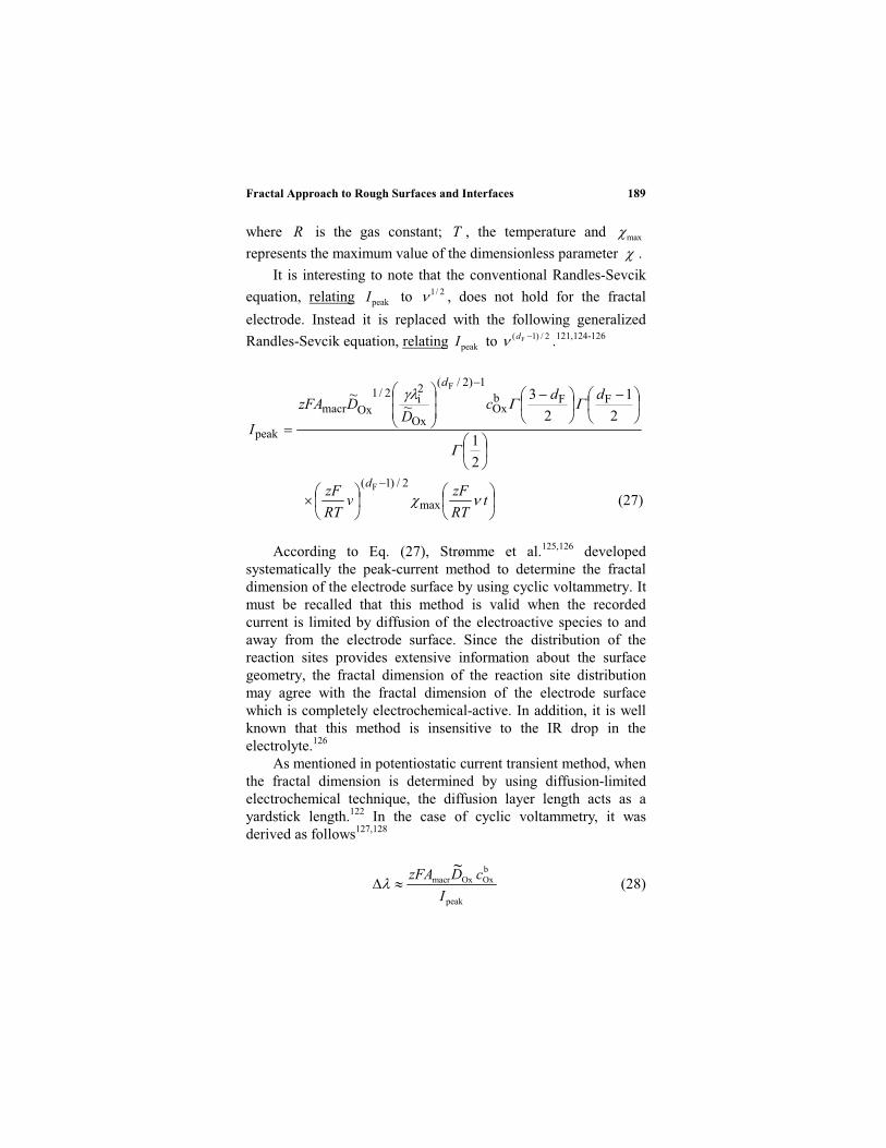
Fractal Approach to Rough Surfaces and Interfaces 189
where R is the gas constant; T , the temperature and max
represents the maximum value of the dimensionless parameter .
It is interesting to note that the conventional Randles-Sevcik
equation, relating peakI to 2/1 , does not hold for the fractal
electrode. Instead it is replaced with the following generalized
Randles-Sevcik equation, relating peakI to 2/)1( Fd .121,124-126
(27)
2
1
2
1
2
3~
~
max
2/)1(
FFbOx
1)2/(
Ox
2i2/1
Oxmacr
peak
F
F
tRT
zFv
RT
zF
ddc
DDzFA
I
d
d
According to Eq. (27), Strømme et al.125,126 developedsystematically the peak-current method to determine the fractaldimension of the electrode surface by using cyclic voltammetry. Itmust be recalled that this method is valid when the recordedcurrent is limited by diffusion of the electroactive species to andaway from the electrode surface. Since the distribution of thereaction sites provides extensive information about the surfacegeometry, the fractal dimension of the reaction site distributionmay agree with the fractal dimension of the electrode surfacewhich is completely electrochemical-active. In addition, it is wellknown that this method is insensitive to the IR drop in theelectrolyte.126
As mentioned in potentiostatic current transient method, whenthe fractal dimension is determined by using diffusion-limitedelectrochemical technique, the diffusion layer length acts as ayardstick length.122 In the case of cyclic voltammetry, it wasderived as follows127,128
peak
bOxOxmacr
I
cDzFA~
(28)

Joo–Young Go and Su-Il Pyun190
where is the diffusion layer length.Therefore, we can define a length scale range where the rough
surface shows the fractal behavior by determining the inner andouter cutoffs using Eq. (28).121 In other words the fractaldimensions determined from the power relation between peakI and
in the cyclic voltammetry have a physical meaning in the rangebetween the inner cutoff and the outer cutoff.
If the capacitive current exists significantly in redox system, itis necessary to remove the effect of capacitive current on peakI for
the accurate determination of Fd . In addition, since this effect is
larger with increasing potential scan rate, regardless of the surfaceroughness of the electrode surface, the inner cutoff determined byusing Eq. (28) might include some ambiguity.
(iii) Ac Impedance Spectroscopy
A constant phase element (CPE) rather than the idealcapacitance is normally observed in the impedance of electrodes.In the absence of Faradaic reactions, the impedance spectrumdeviates from the purely capacitive behavior of the blockingelectrode, whereas in the presence of Faradaic reactions, the shapeof the impedance spectrum is a depressed arc. The CPE showspower law frequency dependence as follows129,130
CPE)(1
)( jB
Z (29)
where B means the CPE coefficient; j , the imaginary unit;
CPE , the CPE exponent; Z , the impedance and represents the
angular frequency.Considerable effort has been made to understand the origin of
the CPE. One of the most possible causes of the CPE is ofgeometric origin: an irregular and porous electrode geometrycauses current density inhomogeneities and thus yields deviationsfrom ideal behavior. A number of theoretical papers131-144 haveinvestigated the relationship between the fractal geometry of the
Fractal Approach to Rough Surfaces and Interfaces 191
electrode and the CPE exponent CPE . Pajkossy and Nyikos144
have shown that for a self-similar fractal working electrode with02F .d , and when the counter electrode is located far from the
working electrode, the relationship between Fd and CPE is given
as
1
1
FCPE
d(30)
However, the relationship between Fd and CPE is dependent on
the model used in the fractal characterization of theelectrode.144,145
Furthermore, it has been reported that the CPE originatedfrom the surface inhomogeneities and adsorption effects ratherthan the irregular geometry because the CPE due to irregulargeometry appears at much higher frequencies than is usual inelectrochemical methodologies.145-147 Therefore, for the reliablefractal characterization of electrode surface in terms of CPE , it
must be rigorously checked whether the surface state of theelectrode is homogeneous or not and whether the effect of thesurface roughness on the CPE dominates the surfaceinhomogeneities and adsorption effects or not.
The length scales corresponding to the frequency rangeswhere the fractal scaling property is expected in the impedancemeasurements can be considered. According to Pajkossy,145 therelationship between the length scale and the frequency f is
give as
ele2
1
Cf (31)
where eC means the electrode capacitance per unit area and el is
the specific resistivity of the electrolyte.

Joo–Young Go and Su-Il Pyun192
IV. INVESTIGATION OF DIFFUSION TOWARDS
SELF-AFFINE FRACTAL INTERFACE
Since diffusing species move randomly in all directions, thediffusing species may sense the self-affine fractal surface and theself-similar fractal surface in quite different ways. Nevertheless alittle attention has been paid to diffusion towards self-affine fractalelectrodes. Only a few researchers have realized this problem:Borosy et al.148 reported that diffusion towards self-affine fractalsurface leads to the conventional Cottrell relation rather than thegeneralized Cottrell relation, and Kant149,150 discussed theanomalous current transient behavior of the self-affine fractalsurface in terms of power spectral density of the surface.
Recently, Pyun et al.43,45 gave a clear interpretation ofdiffusion towards self-affine fractal interface. They investigatedtheoretically how the diffusing ions sense the self-affine fractalinterface during the diffusion-limited process43 and then providedsuccessful experimental evidence of the theoretical investigation.45
Here, let us explore their works in detail.In their theoretical work,43 the various self-affine fractal
interfaces were mathematically constructed employing theWeierstrass function )(WS xf .151,152
N
k
kk xbaxf1
WS )cos()( (32)
where ba 10 with 1ab . The curve )(WS xf is known to
have the following value for the self-affine fractal dimension
saF,d :
b
ad
ln
ln2saF, (33)
A self-affine fractal profile with 51saF, .d was obtained by
taking a , b , and N as 0.8165, 1.5, and 50, respectively. Next,various affine functions )(xh were made by multiplying )(WS xf
Fractal Approach to Rough Surfaces and Interfaces 193
by morphological amplitude (=0.1, 0.3, 0.5, 1.0, 2.0, and 4.0),
..ei , )()( WS xfxh . The resulting six self-affine functions are
presented in Figure 7. Here, it should be noted that the originalself-affine function )(WS xf and the magnified functions )(xh
have the same self-affine fractal dimension 51saF, .d , but they
are quite different from each other in the amplitude.In order to examine the current response to the imposition of
the potential step on the self-affine fractal interface, the currenttransients were calculated theoretically by random walksimulation.153 The simulation cell was taken as the square areabottom boundary which is replaced by one of the self-affine fractalprofiles in Figure 7. The details of the simulation condition weredescribed in their publication.43
Figures 8a and 8b present the simulated current transientsobtained from the self-affine fractal interfaces of 5.0;3.0;1.0
and 0.4;0.2;0.1 , respectively, embedded by the Euclidean
two-dimensional space. It is well known that the current-timerelation during the current transient experiment is expressed as thegeneralized Cottrell equation of Eqs. (16) and (24).154 So, thepower exponent should have the value of - 0.75 for all theabove self-affine fractal interfaces.
However, the simulated current transients in Figure 8 neverexhibited the expected power exponent of –0.75 with theexception of the original self-affine fractal interface ( 1 ): the
simulated current transients showed more negative powerdependence with increasing of the interface before the temporal
outer (longer) cutoff of fractality,121,155 followed by the powerdependence of - 0.5. In addition, in the case of relatively largeamplitudes ( 02. and 4.0), the current transients were roughly
characterized by two-stage power dependence before the temporalouter (longer) cutoff of fractality.
This result strongly indicates that the self-affine fractaldimension saF,d is not always sufficient to describe the
atomic/ionic diffusion of the self-affine fractal interface and at thesame time the morphological amplitude of the interfaceadditionally plays an important role in current transient behavior.
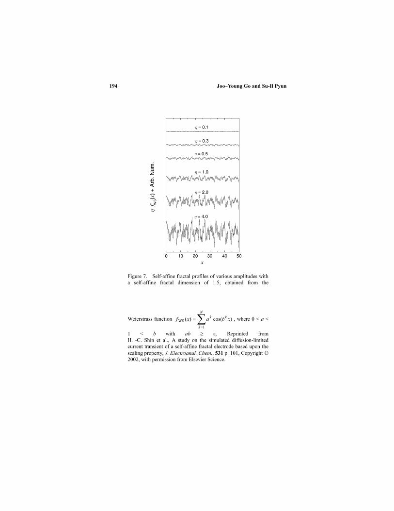
Joo–Young Go and Su-Il Pyun194
Figure 7. Self-affine fractal profiles of various amplitudes witha self-affine fractal dimension of 1.5, obtained from the
Weierstrass function N
k
kk xbaxf
1
WS )cos()( , where 0 < a <
1 < b with ab a. Reprinted fromH. -C. Shin et al., A study on the simulated diffusion-limitedcurrent transient of a self-affine fractal electrode based upon thescaling property, J. Electroanal. Chem., 531 p. 101, Copyright 2002, with permission from Elsevier Science.
40 503020100
= 0.1
= 0.3
= 0.5
= 2.0
= 4.0
= 1.0
f WS( x
) +
Arb
. Num
.
x

Fractal Approach to Rough Surfaces and Interfaces 195
Figure 8. Simulated current transients obtained from theself-affine fractal profiles h(x) of various morphologicalamplitudes of: (a) 0.1, 0.3, and 0.5; (b) 1.0, 2.0, and 4.0in h(x) = fWS(x). Reprinted from H.-C. Shin et al., A studyon the simulated diffusion-limited current transient of aself-affine fractal electrode based upon the scaling property,J. Electroanal. Chem., 531, p. 101, Copyright 2002, withpermission from Elsevier Science.

Joo–Young Go and Su-Il Pyun196
Figure 9. Dependence of the scaled length SL on the projected segment sizeSS on a logarithmic scale obtained from the self-affine fractal profiles in Figure7 by using the triangulation method for Euclidean two-dimensional space.Here, s means d ln SL / d ln SS. Reprinted from H. -C. Shin et al., A study onthe simulated diffusion-limited current transient of a self-affine fractalelectrode based upon the scaling property, J. Electroanal. Chem. 531, p. 101,Copyright 2002, with permission from Elsevier Science.
It should be stressed here that the specific power dependencesfrom the above self-affine fractal interfaces are maintained evenduring the relatively long time (or number of random jumps)interval. This implies that the morphology of the self-affine fractalinterfaces tested is possibly characterized by the self-similarfractal dimension within a relatively wide spatial cutoff range.
Two-stage power dependence at 01. further implies that
local small irregularity regions, i.e., the regions with high
103
102
10-1 1 10
SST
= 0.1 = 0.3 = 0.5 = 1.0
= 2.0
= 4.0
dF,ss
= - (d ln SL / d ln SS) + 1 = - s + 1
s = - 0.042+ 0.004
s = - 0.211+ 0.018
s = - 0.336+ 0.019
s = - 0.483+ 0.012
s = - 0.606+ 0.075
s = - 0.561+ 0.023
s = - 0.923+ 0.132
s = - 0.599+ 0.025
Sca
led
Leng
th S
L
Segment Size SS

Fractal Approach to Rough Surfaces and Interfaces 197
curvature, have a different self-similar scaling property from locallarge irregularity regions, i.e., the regions with low curvature, aftermagnification process: local small irregularity regions seem to beless sensitive to vertical magnification than local large irregularityregions. This can be easily justified in a geometrical point of viewby scaling property analysis for magnified curves (see Figure 9).At this point, one could predict two-stage power dependence evenat 01. . In this case, the second power exponent should be the
value between the first power exponent and - 0.5 according to theabove. Unfortunately, the ambiguity of the current transient due totransition of fractality to non-fractality in the vicinity of thepossible second power dependence region hinders us and one hasto estimate the second power exponent in this region.
Under the assumption that the morphology of the self-affineinterface has the self-similar scaling property, the apparent self-similar fractal dimension ssF,d of the electrode was calculated
from the current transients in Figure 8 by Eqs. (16) and (24). Theresulting fractal dimension is listed in Table 1 (2nd column).
Table 1
Fractal Dimensions of the Profiles h(x) at Various
Morphological Amplitudes in h(x) = fWS(x)
Determined by the Current Transient Technique (2nd
Column) and the Triangulation Method (3rd Column).
Here, fWS(x) Means the Weierstrass Function with a Self-
Affine Fractal Dimension dF,sa = 1.5a
dFdF
Determined by thecurrent transient technique
dF,ss
Determined by thetriangulation method
0.1 1.050 ± 0.020 1.042 ± 0.0040.3 1.258 ± 0.008 1.211 ± 0.0180.5 1.368 ± 0.006 1.336 ± 0.0191.0 1.524 ± 0.004 1.483 ± 0.0122.0 1.588 ± 0.010; 1.770 ± 0.010 1.561 ± 0.023; 1.606 ± 0.0754.0 1.682 ± 0.004; 1.968 ± 0.014 1.599 ± 0.025; 1.923 ± 0.132
a Reprinted from H. -C. Shin et al., A Study on the Simulated Diffusion-Limited Current Transient of a Self-Affine Fractal Electrode Based Uponthe Scaling Property, J. Electroanal. Chem. 531, p. 101, Copyright 2002, with Permission from Elsevier Science.

Joo–Young Go and Su-Il Pyun198
Now, it is necessary to check the self-similar scalingproperties of the original and the magnified self-affine fractalprofiles )(xh of Figure 7. For this purpose, the profiles were
analyzed by the triangulation method. The analysis of a fractalcurve embedded in the Euclidean two-dimensional space by thetriangulation method is performed in the following manner: thecurve with a width L is first divided into N equal segments (thenthe segment size SS becomes NL / ). Next, the scaled length SLof the curve is calculated by
1
0
2122
1SLN
i N
Li
N
Lhi
N
Lh
/
)( (34)
The above operation is iterated at various segment sizes.Finally, the self-similar fractal dimension of the profile embeddedby the two-dimensional space is given by
1SSlnd
SLlndssF,d (35)
Figure 9 demonstrates the dependence of the scaled length SLon the segment size SS obtained from the self-affine fractalprofiles in Figure 7 by using the triangulation method for theEuclidean two-dimensional space. The linear relation was clearlyobserved for all the self-affine fractal curves, which is indicativeof the self-similar scaling property of the curves.
The self-similar fractal dimension determined from Figure 9by Eq. (35) is listed in Table 1 (3rd column). The values of ssF,d
obtained from the simulated current transients of Figure 8 sharedvery well with those values determined by the triangulationmethod. Moreover, the temporal transition point, e.g.,
900triT, at 04. , estimated from the spatial transition point,
05.1SST at 0.4 , from the first linearity (self-similar region)
to the second linearity (self-similar region) in Figure 9 by the
approximate relation DSS 2/2TT (where D is random diffusion
coefficient) quantitatively coincided well with that temporal

Fractal Approach to Rough Surfaces and Interfaces 199
transition point, 700curT, at 0.4 , in the current transients
in Figure 8, which justifies their analysis.From the above results, it is noted that the self-similar scaling
property investigated by the triangulation method can beeffectively utilized to analyze the diffusion towards the self-affinefractal interface. This is the first attempt to relate the powerdependence of the current transient obtained from the self-affinefractal curve to the self-similar scaling properties of the curve.
This theoretical result was experimentally confirmed with thehelp of AFM and cyclic voltammetry by Go et al.45 In that work,they first prepared three kinds of self-affine fractal Pt filmelectrodes by dc sputtering of Pt on three kinds of substrates withdifferent roughnesses. And then, surface morphologies of the threeelectrode specimens were examined by using AFM, and the cyclicvoltammograms were obtained from the electrode specimens atvarious scan rates. Finally, the fractal dimensions of the electrodesurfaces were determined from the analyses of the AFM image byboth the perimeter-area method and the triangulation method andalso from the analysis of the cyclic voltammograms by the peak-current method, and the resulting fractal dimensions werecompared with one another.
Figures 10a, 10b, and 10c illustrate the surface morphologiesof Pt/polished 32OAl , Pt/etched Ni and Pt/unpolished 32OAl
electrodes, respectively, investigated with AFM. The three-dimensional AFM image of Pt/polished 32OAl electrode shows a
very flat surface. However, the three-dimensional AFM images ofPt/etched Ni electrode and Pt/unpolished 32OAl electrode show
the coarse and scratched protrusions with a lateral extent of20–40 m and the small and rounded protrusions with a lateralextent of 1–5 m, respectively. These morphologies of the Ptfilms are characteristic of the bare surface of the substrates:polished 32OAl , etched Ni, and unpolished 32OAl .
To quantitatively characterize the surface roughness of the Ptfilms, the rms roughness rms of the electrodes was evaluated and
the resulting values are indicated in Figures 10a, 10b and 10c,respectively. From the comparison between rms and the scan size
in value, it is indicated that the height fluctuation of all the film

Joo–Young Go and Su-Il Pyun200
Figure 10. Three-dimensional AFM images of (a) Pt/polished Al2O3, (b)Pt/etched Ni, and (c) Pt/unpolished Al2O3 electrodes. Reprinted from J. -Y. Go etal., A study on ionic diffusion towards self-affine fractal electrode by cyclicvoltammetry and atomic force microscopy, J. Electroanal. Chem., 549, p. 49,Copyright 2003, with permission from Elsevier Science.
(a) Pt/polished Al2O3
(b) Pt/etched Ni
(c) Pt/unpolished Al2O3
µm
µm
µm
µmµm
µm
µmµm
µm
rms roughness= 0.012 µm
rms roughness= 0.799 µm
rms roughness= 0.481 µm
5
5
5
050
4540
3530
2520
1510
50 0
510
1520
2530
3540
4550
090
8070
6050
4030
2010
0 010
2030
4050
6070
8090
025
20
15
10
5
0 0
5
10
15
20
25
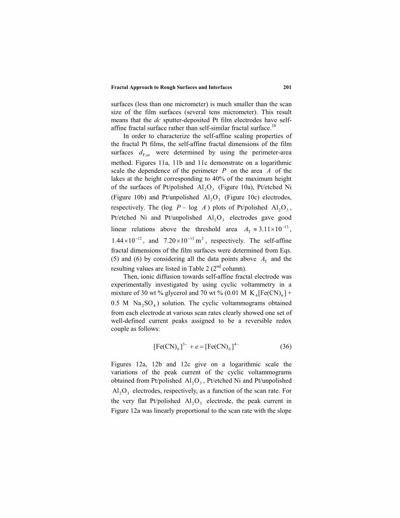
Fractal Approach to Rough Surfaces and Interfaces 201
surfaces (less than one micrometer) is much smaller than the scansize of the film surfaces (several tens micrometer). This resultmeans that the dc sputter-deposited Pt film electrodes have self-affine fractal surface rather than self-similar fractal surface.10
In order to characterize the self-affine scaling properties ofthe fractal Pt films, the self-affine fractal dimensions of the filmsurfaces saF,d were determined by using the perimeter-area
method. Figures 11a, 11b and 11c demonstrate on a logarithmicscale the dependence of the perimeter P on the area A of thelakes at the height corresponding to 40% of the maximum heightof the surfaces of Pt/polished 32OAl (Figure 10a), Pt/etched Ni
(Figure 10b) and Pt/unpolished 32OAl (Figure 10c) electrodes,
respectively. The (log P – log A ) plots of Pt/polished 32OAl ,
Pt/etched Ni and Pt/unpolished 32OAl electrodes gave good
linear relations above the threshold area 13T 1011.3A ,
121044.1 , and 213 m1020.7 , respectively. The self-affine
fractal dimensions of the film surfaces were determined from Eqs.(5) and (6) by considering all the data points above TA and the
resulting values are listed in Table 2 (2nd column).Then, ionic diffusion towards self-affine fractal electrode was
experimentally investigated by using cyclic voltammetry in amixture of 30 wt % glycerol and 70 wt % (0.01 M ][Fe(CN)K 64 +
0.5 M 42SONa ) solution. The cyclic voltammograms obtained
from each electrode at various scan rates clearly showed one set ofwell-defined current peaks assigned to be a reversible redoxcouple as follows:
46
36 ])Fe(CN[])CN(Fe[ e (36)
Figures 12a, 12b and 12c give on a logarithmic scale thevariations of the peak current of the cyclic voltammogramsobtained from Pt/polished 32OAl , Pt/etched Ni and Pt/unpolished
32OAl electrodes, respectively, as a function of the scan rate. For
the very flat Pt/polished 32OAl electrode, the peak current in
Figure 12a was linearly proportional to the scan rate with the slope

Joo–Young Go and Su-Il Pyun202
of 0.500 at all scan rates below the upper threshold scan rate i .
However, in the case of rough Pt/etched Ni and Pt/unpolished
32OAl electrodes, the peak currents in Figures 12b and 12c were
linearly proportional to the scan rates with the slope of 0.512 and0.529, respectively, within the scan rate range of the lowerthreshold scan rate o to the upper threshold scan rate i . It is
noted that the temporal inner (short) cutoff i and outer (longer)
cutoff o correspond to the upper threshold scan rate i and the
lower threshold scan rate o , respectively.
Figure 11. Dependence of the perimeter P on the area A of thelakes on a logarithmic scale obtained at a heightcorresponding to 40% of the maximum height of the surfacesof (a) Pt/polished AL2O3, (b) Pt/etched Ni, and (c)Pt/unpolished Al2O3 electrodes. The slope s means (d log P /d log A). Reprinted from J. -Y. Go et al., A study on ionicdiffusion towards self-affine fractal electrode by cyclicvoltammetry and atomic force microscopy, J. Electroanal.
Chem., 549 p. 49, Copyright 2003, with permission fromElsevier Science.
10-2 10-1 1 10110-1
1
101
102
AT
dF, sa
= 2 (d log P / d log A) + 1 = 2 s + 1
Pt/polished Al2O
3
s = 0.544 + 0.100d
F,sa = 2.088 + 0.200
nophysicalmeaning
Per
imet
erP
/ m
Area A / m2
(a)
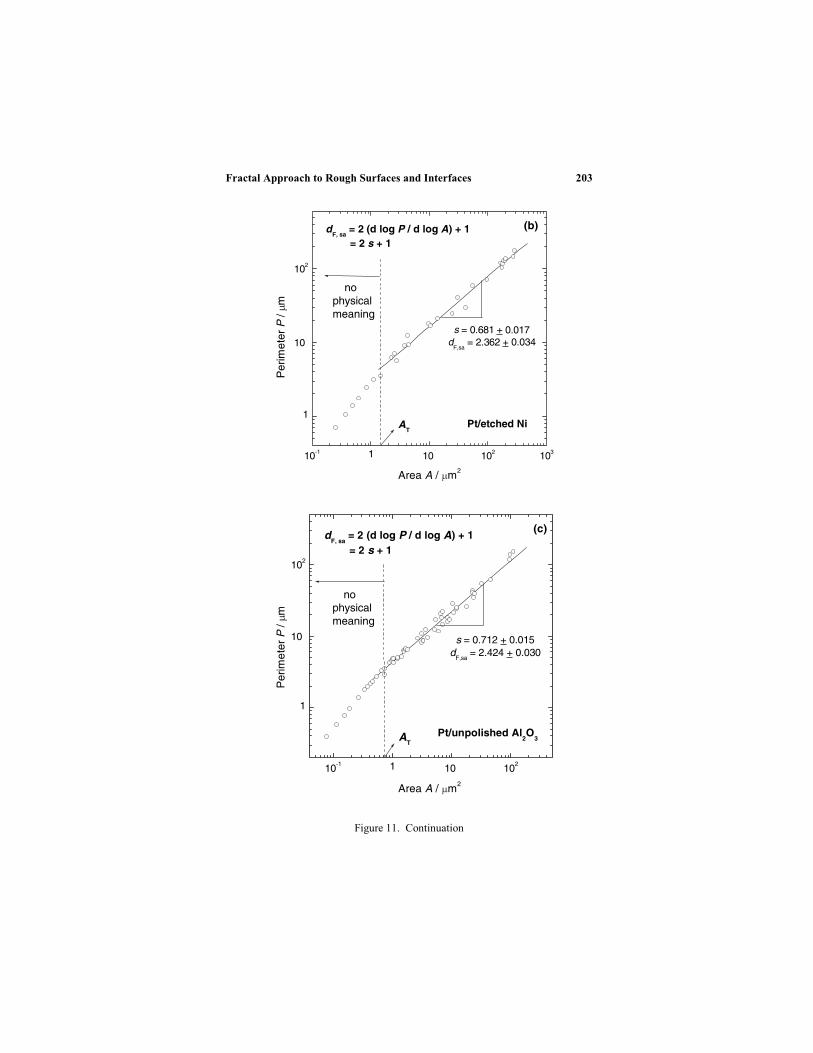
Fractal Approach to Rough Surfaces and Interfaces 203
Figure 11. Continuation
10-1 1 101 102 103
1
101
102
AT
dF, sa
= 2 (d log P / d log A) + 1 = 2 s + 1
Pt/etched Ni
s = 0.681 + 0.017d
F,sa = 2.362 + 0.034
nophysicalmeaning
physicalmeaning
Per
imet
er P
/ m
Per
imet
er P
/ m
Area A / m2
Area A / m2
10-1 1 101 102
1
101
102
AT
dF, sa
= 2 (d log P / d log A) + 1 = 2 s + 1
Pt/unpolished Al2O
3
s = 0.712 + 0.015d
F,sa = 2.424 + 0.030
no
(b)
(c)

Joo–Young Go and Su-Il Pyun204
Keeping in mind that the dc sputter-deposited Pt films havethe completely electrochemical-active surface, the fractaldimensions of the rough film surfaces were calculated from Eq.(27) according to the peak-current method by taking the slopes ofthe (log peakI – log ) plots within the scan rate range of o to
i . The resulting fractal dimensions are listed with the dimension
of the flat film surface in Table 2 (3rd column).
Figure 12. Dependence of the anodic peak current Ipeak on thepotential scan rate on a logarithmic scale obtained from thecyclic voltammograms for (a) Pt/polished Al2O3, (b) Pt/etchedNi, and (c) Pt/unpolished Al2O3 electrodes. The slope means (dlog Ipeak / d log ). Here, i and o means the upper and lowerthreshold scan rate, respectively. Reprinted from J. -Y. Go et al.,A study on ionic diffusion towards self-affine fractal electrode bycyclic voltammetry and atomic force microscopy, J. Electroanal.
Chem. 549, p. 49, Copyright 2003, with permission fromElsevier Science.
103 104
104.00
103.80
103.60
103.40
i
dF = 2 (d log I
peak / d log ) + 1
= 2 + 1
Pt/polished Al2O
3
= 0.500 + 0.002d
F = 2.000 + 0.004
Pea
k C
urre
nt I pe
ak /
A
Scan Rate / mV s-1
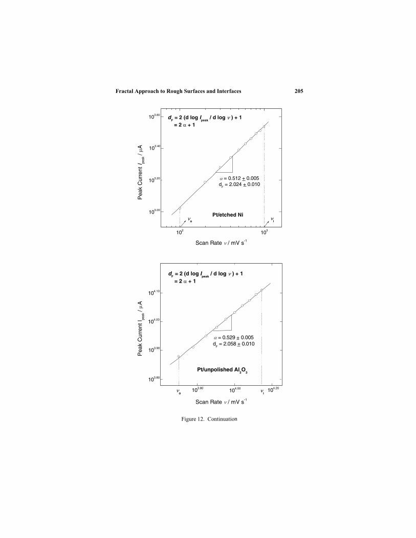
Fractal Approach to Rough Surfaces and Interfaces 205
Figure 12. Continuation
102 103
103.40
103.60
103.20
103.00
dF = 2 (d log I
peak / d log ) + 1
= 2 + 1
io
Pt/etched Ni
= 0.512 + 0.005d
F = 2.024 + 0.010
104.20104.00
104.10
104.00
103.80
103.90
103.80
dF = 2 (d log I
peak / d log ) + 1
= 2 + 1
io
Pt/unpolished Al2O
3
= 0.529 + 0.005d
F = 2.058 + 0.010
Pea
k C
urre
nt I pe
ak /
AP
eak
Cur
rent
I peak
/ A
Scan Rate / mV s-1
Scan Rate / mV s-1
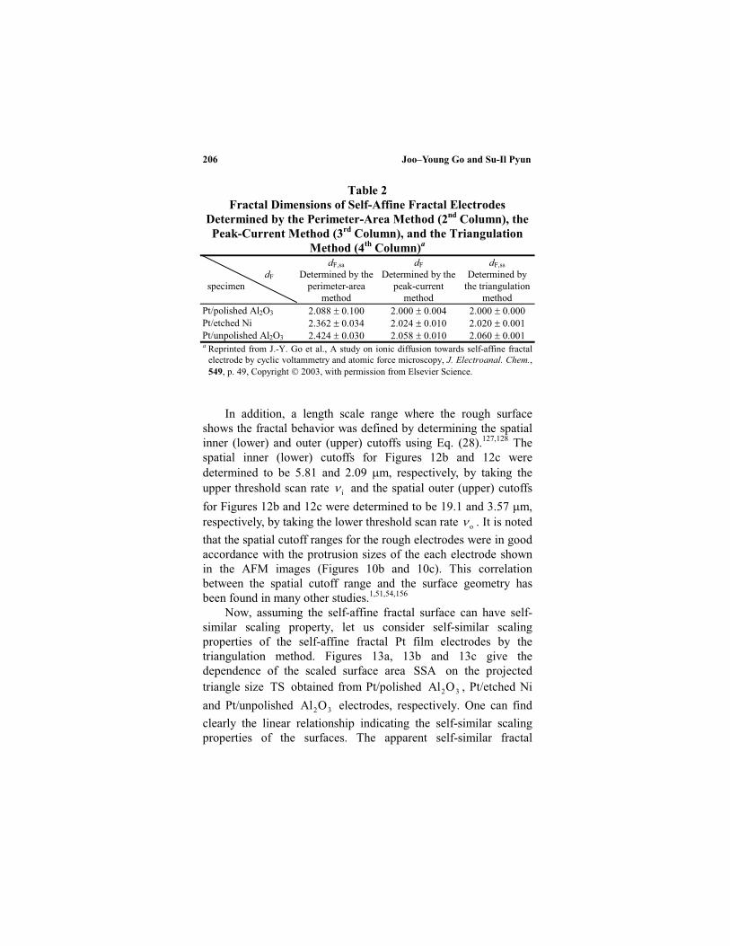
Joo–Young Go and Su-Il Pyun206
Table 2
Fractal Dimensions of Self-Affine Fractal Electrodes
Determined by the Perimeter-Area Method (2nd
Column), the
Peak-Current Method (3rd
Column), and the Triangulation
Method (4th
Column)a
dF
specimen
dF,sa
Determined by theperimeter-area
method
dF
Determined by thepeak-current
method
dF,ss
Determined bythe triangulation
methodPt/polished Al2O3 2.088 0.100 2.000 0.004 2.000 0.000Pt/etched Ni 2.362 0.034 2.024 0.010 2.020 0.001Pt/unpolished Al2O3 2.424 0.030 2.058 0.010 2.060 0.001a Reprinted from J.-Y. Go et al., A study on ionic diffusion towards self-affine fractal
electrode by cyclic voltammetry and atomic force microscopy, J. Electroanal. Chem.,549, p. 49, Copyright 2003, with permission from Elsevier Science.
In addition, a length scale range where the rough surfaceshows the fractal behavior was defined by determining the spatialinner (lower) and outer (upper) cutoffs using Eq. (28).127,128 Thespatial inner (lower) cutoffs for Figures 12b and 12c weredetermined to be 5.81 and 2.09 m, respectively, by taking theupper threshold scan rate i and the spatial outer (upper) cutoffs
for Figures 12b and 12c were determined to be 19.1 and 3.57 m,respectively, by taking the lower threshold scan rate o . It is noted
that the spatial cutoff ranges for the rough electrodes were in goodaccordance with the protrusion sizes of the each electrode shownin the AFM images (Figures 10b and 10c). This correlationbetween the spatial cutoff range and the surface geometry hasbeen found in many other studies.1,51,54,156
Now, assuming the self-affine fractal surface can have self-similar scaling property, let us consider self-similar scalingproperties of the self-affine fractal Pt film electrodes by thetriangulation method. Figures 13a, 13b and 13c give thedependence of the scaled surface area SSA on the projectedtriangle size TS obtained from Pt/polished 32OAl , Pt/etched Ni
and Pt/unpolished 32OAl electrodes, respectively. One can find
clearly the linear relationship indicating the self-similar scalingproperties of the surfaces. The apparent self-similar fractal
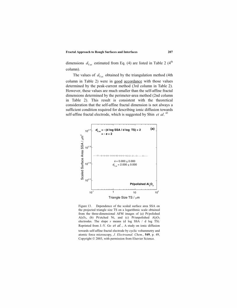
Fractal Approach to Rough Surfaces and Interfaces 207
dimensions ssF,d estimated from Eq. (4) are listed in Table 2 (4th
column).
The values of ssF,d obtained by the triangulation method (4th
column in Table 2) were in good accordance with those valuesdetermined by the peak-current method (3rd column in Table 2).However, these values are much smaller than the self-affine fractaldimensions determined by the perimeter-area method (2nd columnin Table 2). This result is consistent with the theoreticalconsideration that the self-affine fractal dimension is not always asufficient condition required for describing ionic diffusion towardsself-affine fractal electrode, which is suggested by Shin .alet
43
Figure 13. Dependence of the scaled surface area SSA onthe projected triangle size TS on a logarithmic scale obtainedfrom the three-dimensional AFM images of (a) Pt/polishedAl2O3, (b) Pt/etched Ni, and (c) Pt/unpolished Al2O3
electrodes. The slope s means (d log SSA / d log TS).Reprinted from J.-Y. Go .alet , A study on ionic diffusion
towards self-affine fractal electrode by cyclic voltammetry andatomic force microscopy, J. Electroanal. Chem., 549, p. 49,Copyright 2003, with permission from Elsevier Science.
10-1 1 10 102
102.77
102.75
102.73
102.71
dF,ss
= - (d log SSA / d log TS) + 2 = - s + 2
s = 0.000 + 0.000d
F,ss = 2.000 + 0.000
Pt/polished Al2O
3
Sca
led
Sur
face
Are
a S
SA
/ m
2
Triangle Size TS / m
(a)
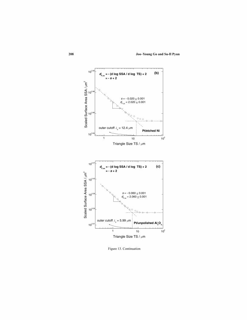
Joo–Young Go and Su-Il Pyun208
Figure 13. Continuation
1 101 102
103.90
103.88
103.86
103.84
outer cutoff o = 12.4 m
dF,ss
= - (d log SSA / d log TS) + 2= - s + 2
s = - 0.020 + 0.001d
F,ss = 2.020 + 0.001
Pt/etched Ni
Sca
led
Sur
face
Are
a S
SA
/ m
2
Triangle Size TS / m
1 101 102
103.47
103.43
103.39
103.35
103.31
outer cutoff o = 5.99 m
dF,ss
= - (d log SSA / d log TS) + 2= - s + 2
s = - 0.060 + 0.001d
F,ss = 2.060 + 0.001
Pt/unpolished Al2O
3
Sca
led
Sur
face
Are
a S
SA
/ m
2
Triangle Size TS / m
(b)
(c)
Fractal Approach to Rough Surfaces and Interfaces 209
Bearing in mind that diffusing ions move randomly in alldirections, it is reasonable to say that the diffusing ions sense self-similar scaling property of the electrode surface irrespective ofwhether the fractal surface has self-similar scaling property orself-affine scaling property. Therefore, it is experimentallyjustified that the fractal dimension of the self-affine fractal surfacedetermined by using the diffusion-limited electrochemicaltechnique represents the apparent self-similar fractal dimension.43
In summary, from the above theoretical and experimentalresults, it is concluded that ionic diffusion towards self-affinefractal electrode should be described in terms of the apparent self-similar fractal dimension rather than the self-affine fractaldimension. In addition, the triangulation method is one of the mosteffective methods to characterize the self-similar scaling propertyof the self-affine fractal electrode.
V. APPLICATION OF THE FRACTAL GEOMETRY IN
ELECTROCHEMICAL SYSTEM
1. Corroded Surface
Metallic corrosion is an important field of electrochemistry.Electrodissolution occurring on metal surfaces causes varioussurface morphologies. The quantitative characterization of thecorroded surface using fractal geometry is of great interest sincethe structure of the corrosion front is a significant factor affectingthe transport of ions and corrosion products during corrosionprocess. To develop a better understanding of the relation betweenthe irregular corrosion front and the physical and chemicalcorrosion mechanisms, many researchers have devoted their effortto the fractal characterization of the corrosion front.
In earlier studies, the possibilities of the fractal description ofthe irregular corrosion front were investigated by the imageanalysis of the digitized micrographs and photographs. Costa etal.47 studied the shapes of the pits formed on the commercialstainless steel rods, SS 316L, in synthetic ocean water. The self-affine fractal dimension of the pit profiles was evaluated from theanalysis of the digitized SEM micrographs using the structured
Joo–Young Go and Su-Il Pyun210
walk method.157,158 There were two fractal dimensions for therugged structure of the pit on shorter length scales (dF,sa = 1.17)and for the texture of the pit on longer length scales (dF,sa = 1.45).They explained this crossover of the fractality in terms of thephysico-chemical characteristics of the pitting corrosion.
Jøssang and Feder48 demonstrated that the corrosion front of asteel pipe subjected to CO2 pitting corrosion is a self-affinefractal, and that it does not make sense to analyze the self-affinestructure as if it were a self-similar fractal. They three-dimensionally reconstructed the corrosion front by digitizingphotographs of a sequential grinding of the surface, and developedthe image analysis method using height-difference correlationfunctions obtained from the digitized photographs. The Hurstexponents H in the range of 0.8–0.9 were measured, and it variedwith the position of the cut, indicating an inhomogeneouscorrosion front.
In order to overcome the difficulty in the observation of thecorrosion front, Holten et al.49 used the two-dimensional cell inwhich corrosion can take place along only one exposed edge of ametal for the study on the aluminum corrosion in a 1 M NaCl +0.01 M NaOH (pH = 12) electrolyte. The value of H for thealuminum corrosion front was determined to be in the range of 0.6– 0.7 consistently using the three different methods: the width-horizontal length method, the height-difference correlationfunction method, and the power spectrum method. However, thebox-counting method did not give reasonable values of H in theirwork. They extended their approach to zinc and copper, andsimilar results were obtained.
From the above works, it is confirmed that the irregularsurface made by the electrodissolution of the metal can bequantitatively characterized by using self-affine fractal geometry.Based upon this, the pit morphology was extensively investigatedby many researchers using a two-dimensional cell in relation to thepit mechanisms. Balázs and Gouyet50 studied the influence of Cl–
and Fe+3 ions on the morphology of pits grown in aluminum thinfilms in various 1 mM to 1 M NaCl + 0.2 to 10 mM Fe2(SO4)3 +5 mM sulfuric acid solutions. At low Cl– and Fe3+ content (10 mMCl– and 0.2 mM Fe3+), the shape of pit was similar to percolationclusters in the vicinity of the percolation threshold. The fractal

Fractal Approach to Rough Surfaces and Interfaces 211
dimension of this fractal-like pit was determined to be 1.91 ± 0.01by the analysis of the digitized images using the density-densitycorrelation function and this value is close to 1.89, which is justthe fractal dimension of percolation clusters at percolationthreshold in agreement with the suggestion of Sapoval .alet for
an invasion-like corrosion pattern in the plane.159
Recently, Park and Pyun51-53 have intensively investigated theeffect of the solution temperature on the pitting corrosion ofInconel alloy 600 in the Cl–ion-containing thiosulfate solution.From the SEM observation of the pitted surface of alloy 600 givenin Figure 14,51 pit morphology changed from cylindrical shapesdeveloped at 60 oC (Figure 14b) to highly branched shapes formedat 150 oC (Figure 14d). Furthermore, corrosion pits nucleated andfurther grew without any morphological change during the wholepitting process below 200 oC. On the other hand, above 200 oC,the morphology of the pits changed from highly branched shapesin the early stage to widely grooved shapes in the later stage(Figures 14e, 14f, and 14g).
Figure 14. Typical SEM micrographs of pitmorphology on the surface of alloy 600subjected to a constant anodic potential of 0.8V(Ag/AgCl) for 300s in aqueous 0.1 M Na2S2O3
+ 0.1 M NaCl solution at (a) 25o, (b) 60o, (c)100o, (d) 150o, (e) 200o, (f) 250o, and (g) 300oC.Reprinted from J. -J. Park and S. -I. Pyun, Pitformation and growth of alloy 600 in Cl– ion-containing thiosulphate solution at temperatures298-573 K using fractal geometry, Corros. Sci.,45, p. 995, Copyright 2003, with permissionfrom Elsevier Science.
(a)
25 µm
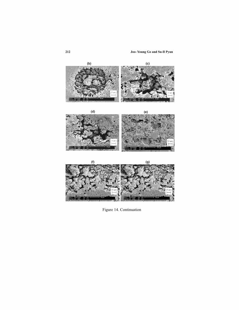
Figure 14. Continuation
Joo–Young Go and Su-Il Pyun212
(b) (c)
(d) (e)
(f) (g)

Fractal Approach to Rough Surfaces and Interfaces 213
In their works,51-54 the self-similar fractal dimension dF,ss ofthe two-dimensional distribution of the pits was determined by theanalysis of the digitized SEM images using the perimeter-areamethod. The value of dF,ss increased with increasing solutiontemperature,51 and it was inversely proportional to the pit shapeparameter and the pit growth rate parameter.53 Keeping in mindthat dF,ss is inversely proportional to the increment of the pit areadensity, these results can be accounted for in terms of the fact thatthe increment of the pit area density is more decelerated withrising solution temperature.
In addition, from the analysis of the ac impedance spectraobtained from the previously pitted surfaces under open circuitconditions at room temperature in 0.5 M Na2SO4 solution51 andfrom the in-situ pitted surfaces in Cl– ion-containing thiosulfatesolution at various applied potentials and solution temperatures,52
they verified that dF,ss is inversely proportional to the CPEexponent for capacitive charging process (Eq. 30)51 and thedepression parameter for charge transfer process.52
The above results concerning the fractal dimension asfunctions of the solution temperature, the CPE exponent, and thedepression parameter are demonstrated again in their otherinvestigation of the effect of the anion addition on pit morphologyof Inconel alloy 600 at elevated temperatures.54
2. Partially Blocked Active Electrode and Active Islands on
Inactive Electrode
Composite electrodes used in the electrochemical processes areoften partially active since they are composed of the activepowder material and the inactive binder and conductor. Thepartially blocked active electrode can be characterized by thecontiguous fractal with dF < 2.0. In the case of the electrodescomposed of the active islands on an inactive support, they arecharacterized by the non-contiguous fractal with dF < 2.0.121
For the contiguous fractal with dF < 2.0, Pajkossy and Nyikosgave the first experimental evidence of the validity of thegeneralized Cottrell equation.121 They prepared two kinds ofpartially active electrodes: a regular fractal pattern with dF =(log 8)/(log 3) 1.893 and a Sierpinski gasket1 with dF =

Joo–Young Go and Su-Il Pyun214
(log 3)/(log 2) 1.585. Then they conducted the potentiostaticcurrent transient experiment on two partially active electrodesusing the diffusion-limited redox couple of K3[Fe(CN)6] andK4[Fe(CN)6]. For both electrodes, the current transients followedexactly the generalized Cottrell behavior of Eqs. (16) and (24).
Subsequently, using a Sierpinski gasket in a gel electrolytecontaining 0.02 M K4[Fe(CN)6] + 0.5 M Na2SO4 solution, Dassasand Duby123 demonstrated experimentally that the transition time
.vs current relationship under galvanostatic control and the peakcurrent .vs potential scan rate relationship in a voltammetricexperiment as well as the current .vs time relationship underpotentiostatic control all followed the power laws with the powerexponent –(dF – 1)/2 according to the analytical solutions to thegeneralized diffusion equation involving a fractional derivativeoperator of Eq. (19).
In practical application, it was reported that the platinumparticles dispersed in highly porous carbonized polyacrylonitrile(PAN) microcellular foam used as fuel-cell electrocatalyst160 havethe partially active property. The fractal dimension of the platinumparticles was determined to be smaller than 2.0 by using thepotentiostatic current transient technique in oxygen-saturatedsolutions, and it was considered to be a reaction dimension,indicating that not all of the platinum particle surface sites areaccessible to the incoming oxygen molecules.
Recently, Lee and Pyun161 have conducted very interestingresearch concerning the morphology of surface groups formed andpoly-vinylidene fluoride (PVDF)-binder materials dispersed onthe graphite composite electrode by using Kelvin probe forcemicroscopy (KFM). They prepared two kinds of electrodes: theas-received SLX50 graphite electrode composed of graphite andPVDF, and the surface-modified SLX50 graphite electrodecomposed of heat-treated graphite, PVDF, and surface groups onthe graphite.
The surface potential profiles of the as-received SLX50graphite electrode (Figure 15a) showed a smooth surface with afew number of broad peaks, but the surface potential profiles ofthe surface-modified SLX50 graphite electrode (Figure 15b)revealed a rough surface with many sharp peaks with lowersurface potential and road peaks with higher surface potential.

Fractal Approach to Rough Surfaces and Interfaces 215
Figure 15. KFM images obtained from the PVDF-bonded composite madefrom (a) the as-received SFG50 graphite and from (b) the surface-modifiedSFG50 graphite. Reprinted from S.-B. Lee and S.-I. Pyun, Determination of themorphology of surface groups formed and PVDF-binder materials dispersed ongraphite composite electrodes in terms of fractal geometry, J. Electroanal.
Chem. 556, p. 75, Copyright 2003, with permission from Elsevier Science.
(b)
(a)

Joo–Young Go and Su-Il Pyun216
Keeping in mind that the surface potential of the PVDF is muchhigher than that surface potential of the surface groups, theyassigned the broad peaks to PVDF and the sharp peaks to surfacegroups.
In order to determine the fractal dimension of the inactive sitedistribution, they cross-sectioned the three-dimensional KFMimages by the planes with constant surface potential. The self-similar distributions of PVDFs on the as-received SFG50 graphiteand the surface-modified SLX50 graphite are given in Figures 16aand 16b, respectively. In addition, the self-similar complexdistribution of surface groups and PVDF on the surface-modifiedSLX50 graphite is shown in Figure 16c. From the analysis of thesecross-sectional images by the perimeter-area method, the self-similar fractal dimensions of PVDF on both electrodes and surfacegroups on the surface-modified SLX50 graphite electrode weredetermined to be about 1.82 ± 0.02 and 1.70 ± 0.02, respectively.
It is of great interest that they distinguished the fractaldimensions of PVDF and surface groups on the surface-modifiedSLX50 graphite by using KFM and that they showed the overallfractal dimension determined by the peak-current method is justthe average of two individual fractal dimensions determined by theKFM analysis. These results indicate that the surface-modifiedSLX50 graphite has multifractal geometry.10
For the non-contiguous fractal with dF < 2.0 as well as thecontiguous one with dF < 2.0, the current response to a potentialstep obeys the generalized Cottrell equation. Pajkossy and Nyikostheoretically elucidated this fact by the random walk simulation ofparticles towards a Cantor-like boundary.121 On the other hand,Strømme et al. experimentally showed the surfaces of theconducting oxide specimens, i.e., In oxide128 and Snoxyfluoride,41,128 are non-contiguous fractal with dF < 2.0. Thenon-contiguously active sites of specimens were visualized by thehillocks on the specimens observed in the AFM image. Then thefractal dimensions of the hillock distribution on the specimensurfaces were obtained from mass-radius analyses performed onthresholded AFM matrices,1,63 and these values agreed with thatfractal dimensions determined by the peak-current method.

Figu
re 1
6.C
ross
-sec
tion
al v
iew
of
the
thre
e-di
men
sion
al K
FM i
mag
e (a
) fo
r th
e as
-rec
eive
d SF
G50
gra
phit
e by
cro
ss-s
ecti
onin
g w
ith
the
plan
eof
the
heig
ht v
alue
in 5
0 %
of
the
max
imum
hei
ght o
f th
e su
rfac
e po
tent
ial,
(b)
for
the
surf
ace-
mod
ifie
d SF
G50
gra
phit
e by
cro
ss-s
ecti
onin
g w
ith
80 %
of
the
max
imum
hei
ght
of t
he s
urfa
ce p
oten
tial
, an
d (c
) fo
r th
e su
rfac
e-m
odif
ied
SFG
50 g
raph
ite
by c
ross
-sec
tion
ing
wit
h 50
% o
f th
em
axim
um h
eigh
t of
the
surf
ace
pote
ntia
l. R
epri
nted
fro
m S
. -B
. Lee
and
S. -
I. P
yun,
Det
erm
inat
ion
of t
he m
orph
olog
y of
sur
face
grou
ps f
orm
edan
d PV
DF-
bind
er m
ater
ials
dis
pers
ed o
n gr
aphi
te c
ompo
site
ele
ctro
des
in te
rms
of f
ract
al g
eom
etry
, J.
Ele
ctro
an
al.
Ch
em.
55
6, p
. 75,
Cop
yrig
ht 2
003,
wit
h pe
rmis
sion
fro
m E
lsev
ier
Scie
nce.
Fractal Approach to Rough Surfaces and Interfaces 217
mm
m
(a)
(b)
(c)
m
50 40 30 20 10
1020
3040
500
0
50 40 30 20 10
1020
3040
500
0
50 40 30 20 10
1020
3040
500
0
Joo–Young Go and Su-Il Pyun218
3. Porous Electrode
Porous materials have attracted considerable attention in theirapplication in electrochemistry due to their large surface area. Asindicated in Section I, there are two conventional definitionsconcerning with the fractality of the porous material, i.e., surfacefractal and pore fractal.9-11 The pore fractal dimension representsthe pore size distribution irregularity: the larger the value of thepore fractal dimension is, the narrower is the pore size distributionwhich exhibits a power law behavior. The pore fractal dimensionsof 2 and 3 indicate the porous electrode with homogeneous poresize distribution and that electrode composed of the almost same-sized pores, respectively.
On the other hand, the surface fractal dimension characterizesthe pore surface irregularity: the larger the value of surface fractaldimension is, the more irregular and the rougher is the poresurface. Since the pore structure is closely related to the electro-active surface area which plays a key role in the increase ofcapacity in practical viewpoint, many researchers haveinvestigated the microstructure of the pores by using fractalgeometry.
Besides the molecular probe method using gasadsorption,107,162 recently, the TEM image analysis method163-167
has been applied to evaluate the surface fractal dimension ofporous materials. The most attractive fact in this method is that thepores in different size ranges can be extracted from the TEMimages which include contributions from many different pore sizesby the inverse fast Fourier transform (FFT) operation by selectingthe specific frequency range.165-167
The pore structure of pitch-based activated carbon fibers werefirst investigated by using the TEM image analysis method.163-166
From the studies on the various activated carbon fibers, it wasshown that the fractal dimension of the pores decrease withprogressing activation processes for the specimen preparation.The fractal dimension obtained by the TEM image analysismethod did not exactly coincide with that fractal dimensionevaluated by the molecular probe method using gas adsorption.Keeping in mind that the TEM image gives direct information ofthe pore structure visually, it was concluded that the fractal

Fractal Approach to Rough Surfaces and Interfaces 219
more accurately reflect the pore properties of the materials thanthe molecular probe method using gas adsorption.
Recently, the mesoporous carbons synthesized by the silicaimprinting method were investigated by using the TEM imageanalysis method and the molecular probe method using gasadsorption.167 In this work, using the TEM image analysis method,two groups of the pores produced from the carbonization ofmesophase pitch and from the silica imprinting were distinguishedin size and the individual fractal dimension were determined.From the comparison of the overall surface fractal dimensionevaluated by the molecular probe method using gas adsorptionwith the individual fractal dimension, it was recognized that theoverall surface fractal dimension is influenced crucially by theindividual dimension of the silica-imprinted pore surface.
VI. CONCLUDING REMARKS
The present article summarized the fractal characterization of therough surfaces and interfaces by using the physical and theelectrochemical methods in electrochemistry. In much research,both the physical and the electrochemical methods were used toevaluate the fractal dimension and they are complementary to eachother. It should be stressed that the surface fractal dimension mustbe determined by using the adequate method, according to theinherent scaling properties of the rough surfaces and interfaces.
Regarding the electrochemical method, the generalized formsof the Cottrell relation and the Randles-Sevcik relation weretheoretically derived from the analytical solutions to thegeneralized diffusion equation involving a fractional derivativeoperator under diffusion-controlled constraints and these areuseful in to determining the surface fractal dimension. It is notedthat ionic diffusion towards self-affine fractal electrode should bedescribed in terms of the apparent self-similar fractal dimensionrather than the self-affine fractal dimension. This means the fractaldimension determined by using the diffusion-limitedelectrochemical method is the self-similar fractal dimensionirrespective of the surface scaling property.
dimension obtained by the TEM image analysis method could

Joo–Young Go and Su-Il Pyun220
However, in the case of the non-diffusion-limitedelectrochemical processes, e.g., cell-impedance-controlled lithiumtransport through transition metal oxides and carbonaceousmaterials168 and hydrogen transport through hydride-formingmetals and alloys,169-171 the generalized relations derived under thediffusion-controlled constraint are not valid any more. Therefore,systematic investigation of diffusion towards fractal interfaceunder the non-diffusion-limited constraint has been necessary forthe wide application of the electrochemical method to fractalcharacterization. Since it is very hard to obtain the analyticalsolutions to the generalized diffusion equation under the non-diffusion-controlled constraint, one of the most useful approachesto diffusion towards fractal interface under the non-diffusion-limited constraint may be the numerical analysis of the generalizeddiffusion equation.
ACKNOWLEDGEMENTS
The receipt of a research grant under the program ‘National R&DProject for Nano Science and Technology’, funded by Ministry ofScience and Technology, Republic of Korea, is gratefullyacknowledged. Furthermore, this work was partly supported bythe Brain Korea 21 project.
NOTATION
a Factor in Weierstrass function
0a Diameter of adsorbed molecule
A Area
cA Effective cross-section area
exA Exposed surface area of the working electrode
macrA Macroscopic area which is defined beyond the
fractal limits
micrA Microscopic area which is defined within the
fractal limits

Fractal Approach to Rough Surfaces and Interfaces 221
TA Threshold area above which the linear relationship
between the logarithm of perimeter and thelogarithm of area appearsPower exponent in the generalized Cottrellequation
CPE CPE exponent
AFM Atomic force microscopeb Factor in Weierstrass functionB CPE coefficient
Proportionality constant in the relationship
between the area and the perimeterB.C. Boundary condition
boxc Bulk concentrationssoxc Surface concentrations
C Power law exponent which is dependent on thesurface fractal dimension determined by thesingle-probe method using gas adsorption
eC Electrode capacitance per unit area
Dimensionless parameter
max Maximum value of
CPE Constant phase element
Ed Topological dimension of the Euclidean space
where the set is embedded
Fd Fractal dimension
BF,d Box dimension
DF,d Divider dimension
MPF,d Surface fractal dimension determined by the
multiprobe method using gas adsorption
saF,d Self-affine fractal dimension
ssF,d Self-similar fractal dimensionL
ssF,d Self-similar fractal dimension of the two-
dimensional self-similar lakes
SF,d Similarity dimension

Joo–Young Go and Su-Il Pyun222
SPF,d Surface fractal dimension determined by the
single-probe method using gas adsorptionD Random diffusion coefficient
Ox
~D Chemical diffusivity of the oxidized species
*Ox
~D Fractional diffusivity
Red
~D Chemical diffusivity of the reduced species
t/ Riemann-Liouville mathematical operator of
fractional derivativeE Electrode potential
2/1E Half-wave potential
iE Initial electrode potential
Threshold for the dominant forces between vander Waals forces and the liquid/gas surface tensionforces in the multilayer gas adsorption
F Faraday constantf Frequency
)(WS xf Weierstrass function
FFT Fast Fourier transformFHH Frenkel, Halsey, and Hill
Dimensionless geometrical parameter
y Gamma function of y
)(xh Affine function
H Hurst exponentMorphological amplitude
I Current
peakI Peak current
I.C. Initial condition
j 1
K Constant related to the fractal dimensionKFM Kelvin probe force microscopyL Length
i Spatial inner (lower) cutoff
o Spatial outer (upper) cutoff

Fractal Approach to Rough Surfaces and Interfaces 223
MP Multiproben Number of adsorbed molecule layersN Number of objects
monoN Number of adsorbed molecules to form a
monolayerPotential scan rate
i Upper threshold scan rate
o Lower threshold scan rate
Ox Oxidized speciesp Adsorption equilibrium pressure of the gas
0p Saturation pressure of the gas
P PerimeterPAN PolyacrylonitrilePVDF Poly-vinylidene fluorider Scaling ratio
)(Sr New set of points at position )( E1 rxrx ...,,x
generated by the similarity transformation of theset S
)...,,( E1 rrr Scaling ratio vector with the different scaling
ratios 1...,,0 E1 rr
)(Sr New set of points at position )( EE11 xrxr ...,,x
generated by the affine transformation of the setS
mr Radius of the sphere probe molecule
R Gas constant
oR Side length of a square electrode
el Specific resistivity of the electrolyte
Red Reduced speciess Slope of the linear lineS Set of points embedded in Euclidean E-
dimensional space at position )( E1 xx ...,,x
N1 ...,, SS Non-overlapping subsets of points, each of which
is congruent to the set generated by the similarityor affine transformations
Diffusion layer length

Joo–Young Go and Su-Il Pyun224
g Generalized Cottrell coefficient
rms Root mean square (rms) roughness
SEM Scanning electron microscopeSL Scaled lengthSP Single-probeSPM Scanning probe microscopeSS Segment size
TSS Spatial transition point in the SSlog .vs SLlog
plotSSA Scaled surface areaSTM Scanning tunneling microscopet Time
adt Actual thickness of adsorbed molecule layers
maxad,t Maximum thickness of adsorbed molecule layers
minad,t Minimum thickness of adsorbed molecule layers
T Temperature (K)
i Temporal inner (shorter) cutoff
o Temporal outer (longer) cutoff
curT, Temporal transition point in the current transient
triT, Temporal transition point corresponding to TSS
TEM Transmission electron microscopeTS Projected triangle sizeV Volume of adsorbed gas molecules
maxV Upper limits of the power-law regimes in the plot
of Vln against )/ln(ln 0 pp
minV Lower limits of the power-law regimes in the plot
of Vln against )/ln(ln 0 pp
monoV Volume of monolayer coverage
Angular frequencyz Number of electrons transferred per the oxidized
species in the redox reactionZ Impedance
Fractal Approach to Rough Surfaces and Interfaces 225
REFERENCES
1B. B. Mandelbrot, The Fractal Geometry of Nature, W.H. Freeman andCompany, New York, 1983.
2H. -O. Peitgen and D. Saupe, Ed., The Science of Fractal Images, SpringerVerlag, New York, 1988.
3C. A. Pickover, Computers, Pattern, Chaos and Beauty, St. Martin’s Press,New York, 1990.
4H.-O. Peitgen, H. Jürgens, and D. Saupe, Fractals for the Classroom:
Introduction to Fractals and Chaos, Springer Verlag, New York, 1992.5 R. N. Mantegna and H. E. Stanley, Nature 376 (1995) 46.6M. H. R. Stanley, L. A. N. Amaral, S. V. Buldyrev, S. Havlin, H. Leschhorn, P.Maass, M. A. Salinger, and H. E. Stanley, Nature 379 (1996) 804.
7H. Takayasu and K. Okuyama, Fractals 6 (1998) 67.8H. Takayasu, M. Takayasu, M. P. Okazaki, K. Marumo, and T. Shimizu, inParadigms of Complexity, Ed. by M.M. Novak, World Scientific, 2000, p. 243.
9P. Pfeifer and M. Obert, in The Fractal Approach to Heterogeneous Chemistry,Ed. by D. Avnir, Wiley, New York, 1989, p. 11.
10 J. C. Russ, Fractal Surfaces, Plenum Press, New York, 1994.11J. -F. Gouyet, M. Rosso, and B. Sapoval, in Fractals and Disordered Systems,
Ed. by A. Bunde and S. Havlin, Springer-Verlag, New York, 1996, p. 263.12R. Brady and R. C. Ball, Nature 309 (1984) 225.13M. Matsushita, M. Sano, Y. Hayakawa, H. Honjo, and Y. Sawada, Phys. Rev.
Lett. 53 (1984) 286.14D. Grier, E. Ben-Jacob, R. Clarke, and L. M. Sander, Phys. Rev. Lett. 56 (1986)
1264. 15P. Meakin, Crit. Rev. Solid State Mater. Sci. 13 (1987) 147. 16R. de Levie, J. Electroanal. Chem. 281 (1990) 1. 17F. Sagues, F. Mass, M. Villarrasa, and J. Costa, J. Electroanal. Chem. 278
(1990) 351. 18J.M. Gómez-Rodríguez, A.M. Baró, and R.C. Salvarezza, J. Vac. Sci. Technol.
B 9 (1991) 495. 19P. Ocon, P. Herrasti, L. Vázquez, R. C. Salvarezza, J. M. Vara, and A. J. Arvia,
J. Electroanal. Chem. 319 (1991) 101. 20J. M. Gómez-Rodríguez, A. M. Baró, L. Vázquez, R. C. Salvarezza, J. M. Vara,
and A. J. Arvia, J. Phys. Chem. 96 (1992) 347.21P. Herrasti, P. Ocón, R. C. Salvarezza, J. M. Vara, L. Viázquez, and A. J. Arvia,
Electrochim. Acta 37 (1992) 2209.22L. Vázquez, R. C. Salvarezza, P. Ocón, P. Herrasti, J. M. Vara, and A. J. Arvia,
Phys. Rev. E 49 (1994) 1507.23P.L. Antonucci, R. Barberi, A.S. Aricò, A. Amoddeo, and V. Antonucci, Mater.
Sci. Eng. B 38 (1996) 9. 24W. Huang and D. B. Hibbert, Physica A 233 (1996) 888.
25T. Kessler, A. Visintin, A. E. Bolzan, G. Andreasen, R. C. Salvarezza, W. E.Triaca, and A. J. Arvia, Langmuir 12 (1996) 6587.
26F. Gobal, K. Malek, M. G. Mahjani, M. Jafarian, and V. Safarnavadeh, Synth.
Met. 108 (2000) 15. 27B. B. Mandelbrot, D. E. Passoja, and A. J. Paullay, Nature 308 (1984) 721.

Joo–Young Go and Su-Il Pyun226
28E. E. Underwood and K. Banerji, Mat. Sci. Eng. 80 (1986) 1. 29C.S. Pande, L.E. Richards, N. Louat, B.D. Dempsey, and A.J. Schwoeble, Acta
Metall. 35 (1987) 1633.30Z. G. Wang, D. L. Chen, X. X. Jiang, S. H. Ai, and C. H. Shih, Scr. Metall. 22
(1988) 827. 31C. W. Lung and S. Z. Zhang, Physica D 38 (1989) 242.
32A. Imre, T. Pajkossy, and L. Nyikos, Acta Metall. Mater. 40 (1992) 1819.33R. F. Voss, R. B. Laibowitz, and E. I. Allessandrini, Phys. Rev. Lett. 49 (1982)
1441.34J. M. Gómez-Rodríguez, A. Asenjo, R. C. Salvarezza, and A. M. Baró,
Ultramicroscopy 42-44 (1992) 1321.35M. V. H. Rao, B. K. Mathur, and K. L. Chopra, Appl. Phys. Lett. 65 (1994)
124. 36L. Spanos and E. A. Irene, J. Vac. Sci. Technol. A 12 (1994) 2646.
37C. Douketis, Z. Wang, T. L. Haslett, and M. Moskovits, Phys. Rev. B 51 (1995)11022.
38G. W. Mbise, G. A. Niklasson, and C. G. Granqvist, Solid State Comm. 97
(1996) 965.39M. C. Salvadori, M. G. Silveira, and M. Cattani, Phys. Rev. E 58 (1998) 6814.40M. U. Kleinke, J. Davalos, C. Polo da Fonseca, and A. Gorenstein, Appl. Phys.
Lett. 74 (1999) 1683.41G. A. Niklasson, D. Rönnow, M. Strømme Mattsson, L. Kullman, H. Nilsson,
and A. Roos, Thin Solid Films 359 (2000) 203.42L. L. G. Silva, N. G. Ferreira, M. E. R. Dotto, and M. U. Kleinke, Appl. Surf.
Sci. 181 (2001) 327.43H. -C. Shin, S. -I. Pyun, and J. -Y. Go, J. Electroanal. Chem. 531 (2002) 101.
44X. Sun, Z. Fu, and Z. Wu, Mater. Charact. 48 (2002) 169. 45J. -Y. Go, S. -I. Pyun, and Y. -D. Hahn, J. Electroanal. Chem. 549 (2003) 49. 46J. -Y. Go and S. -I. Pyun, Electrochim. Acta 49 (2004) 2551. 47J. M. Costa, F. Sagués, and M. Vilarrasa, Corros. Sci. 32 (1991) 665. 48T. Jøssang and J. Feder, Phys. Scr. T44 (1992) 9. 49T. Holten, T. Jøssang, P. Meakin, and J. Feder, Phys. Rev. E 50 (1994) 754. 50L. Balázs and J. -F. Gouyet, Physica A 217 (1995) 319. 51J. -J. Park and S. -I. Pyun, Corros. Sci. 45 (2003) 995. 52J. -J. Park and S. -I. Pyun, J. Solid State Electrochem. 7 (2003) 380. 53J. -J. Park and S. -I. Pyun, Corros. Sci. 46 (2004) 285. 54S. -I. Pyun and J. -J. Park, J. Solid State Electrochem. 8 (2004) 296. 55N. Almqvist, M. Rubel, and E. Franconi, Mater. Sci. Eng. A 201 (1995) 277. 56N. Almqvist, M. Rubel, P. Wienhold, and S. Fredriksson, Thin Solid Films 270
(1995) 426. 57N. Almqvist, Surf. Sci. 355 (1996) 221. 58J. C. Arnault, A. Knoll, E. Smigiel, and A. Cornet, Appl. Surf. Sci. 171 (2001)
189. 59A. Kirbs, R. Lange, B. Nebe, J. Rychly, P. Müller, and U. Beck, Mater. Sci.
Eng. C 23 (2003) 413. 60A. Kirbs, R. Lange, B. Nebe, R. Rychly, A. Baumann, H. -G. Neumann, and U.
Beck, Mater. Sci. Eng. C 23 (2003) 425. 61J. Feder, Fractals, Plenum Press, New York, 1988.

Fractal Approach to Rough Surfaces and Interfaces 227
62R. F. Voss, in Dynamics of Fractal Surfaces, Ed. by F. Family and T. Vicsek,World Scientific, New Jersey, 1991, p. 39.
63A. -L. Barabási and H. E. Stanley, Fractal Concepts in Surface Growth,Cambridge University Press, Cambridge, 1995.
64H. E. Stanley, in Fractals and Disordered Systems, Ed. by A. Bunde and S.Havlin, Springer-Verlag, New York, 1996, p. 1.
65J.F. Gouyet, Physics and Fractal Structures, Springer, New York, 1995. 66B. B. Mandelbrot, in Fractals in Physics, Ed. by L. Pietronero and E. Tosatti,
North-Holland, Amsterdam, 1986, pp. 3, 17, 21. 67T. Vicsek, Fractal Growth Phenomena, 2nd Ed., World Scientific, Singapore,
1991.68A. Majumdar and B. Bhushan, J. Tribol. 112 (1990) 205.69A. Majumdar and C. L. Tien, Wear, 136 (1990) 313.70A. Majumdar and B. Bhushan, in Handbook of Micro/Nano Tribology, Ed. by
B. Bhushan, CRC Press, New York, 1995, p. 109.71T. Silk, Q. Hong, J. Tamm, and R. G. Compton, Syn. Met. 93 (1998) 65.72K. C. Clark, Comput. Geosci. 12 (1986) 713.73J. Liu and T. Furuno, Wood Fiber Sci. 33 (2001) 213.74J. Liu and T. Furuno, Wood Sci. Technol. 36 (2002) 385.75C. -H. Kim and S. -I. Pyun, Electrochim. Acta 48 (2003) 3455.76B. B. Mandelbrot, Phys. Scr. 32 (1985) 257.77R. C. Salavarezza and A. J. Arvia, in Modern Aspects of Electrochemistry, No.
28, Ed. by B.E. Conway, J. O’M. Bockris, and R.E. White, Plenum Press, NewYork, 1995, p. 289.
78V. Lakshminarayanan, R. Srinivasan, D. Chu, and S. Gilman, Surf. Sci. 392
(1997) 44.79A. Majumdar, B. Bhushan, and C. L. Tien, Adv. Inf. Storage Syst. 1 (1991)
231.80P. I. Oden, A. Majumdar, B. Bhushan, A. Padmanabhan, and J. J. Graham, J.
Tribol. 114 (1992) 666.81P. So, E. Barreto, and B. R. Hunt, Phys. Rev. E 60 (1999) 378.82A. K. Bisoi and J. Mishra, Patt. Recog. Lett. 22 (2001) 631.83D. Avnir and D. Farin, J. Chem. Phys. 79 (1983) 3566.84P. Pfeifer and D. Avnir, J. Chem. Phys. 79 (1983) 3558.85P. Pfeifer, D. Avnir, and D. Farin, Surf. Sci. 126 (1983) 569.86D. Avnir, D. Farin, and P. Pfeifer, Nature 308 (1984) 261.87D. Avnir, D. Farin, and P. Pfeifer, J. Colloid Interface Sci. 103 (1985) 112.88D. Farin, S. Pelog, D. Yavin, and D. Avnir, Langmuir 1 (1985) 399.89A. Y. Myer, D. Farin, and D. Avnir, J. Am. Chem. Soc. 108 (1986) 7897.90D. Avnir, J. Am. Chem. Soc. 109 (1987) 2931.91D. Farin and D. Avnir, J. Phys. Chem. 91 (1987) 5517.92D. Farin and D. Avnir, J. Am. Chem. Soc. 110 (1988) 2039.93D. Avnir and M. Jaroniec, Langmuir 5 (1989) 1431.94A. V. Neimark, Adsorpt. Sci. Technol. 7 (1990) 210.95D. K. Ludlow and T.P. Moberg, Anal. Instrum. 19 (1990) 113.96K. Kaneko, Langmuir 7 (1991) 109.97M. Sato, T. Sukegawa, T. Suzuki, S. Hagiwara, and K. Kaneko, Chem. Phys.
Lett. 181 (1991) 526.98D. Avnir, D. Farin, and P. Pfeifer, New J. Chem. 16 (1992) 439.

Joo–Young Go and Su-Il Pyun228
99Y. Lefebvre, S. Lacelle, and C. Jolicoeur, J. Mater. Res. 7 (1992) 1888.100W. C. Conner and C. O. Bennett, J. Chem. Soc., Faraday Trans. 89 (1993)
4109.101K. S. W. Sing, D. H. Evert, R. A. W. Haul, L. Mosocou, R. A. Pierotti, J.
Rouquerol, and T. Siemieniewska, Pure Appl. Chem. 57 (1985) 603.102R. F. Cracknell, P. Gordon, and K. E. Gubbins, J. Phys. Chem. 97 (1993) 494.103K. Kaneko, R. F. Cracknell, and D. Nichlson, Langmuir 10 (1994) 4606.104T. Suzuki, K. Kaneko, N. Setoyama, M. Maddox, and K.E. Gubbins, Carbon 34
(1996) 909.105K. Kaneko, T. Suzuki, and K. Kakei, Langmuir 5 (1989) 879.106K. Kaneko and C. Ishii, Colloids Surf. 67 (1992) 203.107M. Sato, T. Sukegawa, T. Suzuki, and K. Kaneko, J. Phys. Chem. B 101 (1997)
1845.108P. Pfeifer, Y. J. Wu, M. W. Cole, and J. Krim, Phys. Rev. Lett. 62 (1989) 1997.109P. Pfeifer and M.W. Cole, New J. Chem. 14 (1990) 221.110P. Pfeifer, J. Kenntner, and M.W. Cole, in Fundamentals of Adsorption, Ed. by
A.B. Mersmann and S.E. Scholl, American Institute of Chemical Engineers,New York, 1991, p. 689.
111I. M. K. Ismail and P. Pfeifer, Langmuir 10 (1994) 1532.112P. Pfeifer and K. -Y Liu, in Equilibria and Dynamics of Gas Adsorption on
Heterogeneous Solid Surfaces, Ed. by W. Rudzi ski, W.A. Steele, and G.Zgrablich, Elsevier, New York, 1997, p. 625.
113J. Frenkel, Kinetic Theory of Liquids, Clarendon, Oxford, 1946.114G. D. Halsey, J. Chem. Phys. 16 (1948) 931.115T. L. Hill, Adv. Catal. 4 (1952) 211.116M. K. Wu, Aerosol Sci. Technol. 25 (1996) 392.117P. Tang, N. Y. K. Chew, H. K. Chan, and J. A. Raper, Langmuir 19 (2003)
2632.118R. Larraz, Chem. Eng. J. 86 (2002) 309.119A. J. Bard and L. R. Faulkner, Electrochemical Methods: Fundamentals and
Applications, John Wiley and Sons, New York, 1980.120L. Nyikos and T. Pajkossy, Electrochim. Acta 31 (1986) 1347.121T. Pajkossy and L. Nyikos, Electrochim. Acta 34 (1989) 171.122T. Pajkossy, J. Electroanal. Chem. 300 (1991) 1.123Y. Dassas and P. Duby, J. Electrochem. Soc. 142 (1995) 4175.124T. Pajkossy and L. Nyikos, Electrochim. Acta 34 (1989) 181.125M. Strømme, G. A. Niklasson, and C. G. Granqvist, Phys. Rev. B 52 (1995)
14192.126M. Strømme, G. A. Niklasson, and C. G. Granqvist, Solid State Commun. 96
(1995) 151.127M. Strømme, G. A. Niklasson, and C. G. Granqvist, Phys. Rev. B 54 (1996)
2968.128M. Strømme, G. A. Niklasson, and C. G. Granqvist, Phys. Rev. B 54 (1996)
17884.129R. de Levie, Electrochim. Acta 9 (1964) 1231.130R. de Levie, Electrochim. Acta 10 (1965) 113.131A. Le Mehaute and G. Crepy, Solid State Ionics 9&10 (1983) 17.132A. Le Mehaute, J. Stat. Phys. 36 (1984) 665.

Fractal Approach to Rough Surfaces and Interfaces 229
133S. H. Liu, Phys. Rev. Lett. 55 (1985) 529.134L. Nyikos and T. Pajkossy, Electrochim. Acta 30 (1985) 1533.135T. C. Halsey, Phys. Rev. A 35 (1987) 3512.136T. Kaplan, L.J. Gray, and S. H. Liu, Phys. Rev. B 35 (1987) 5379.137B. Sapoval, Solid State Ionics 23 (1987) 253.138Y.T. Chu, Solid State Ionics 26 (1988) 299.139R.M. Hill and L.A. Dissado, Solid State Ionics 26 (1988) 295.140W.H. Mulder and J.H. Sluyters, Electrochim. Acta 33 (1988) 303.141J. C. Wang, Electrochim. Acta 33 (1988) 707.142M. Blunt, J. Phys. A: Math. Gen. 22 (1989) 1179.143A. Maritan and F. Toigo, Electrochim. Acta 35 (1990) 141.144T. Pajkossy and L. Nyikos, Phys. Rev. B 42 (1990) 709.145T. Pajkossy, J. Electroanal. Chem. 364 (1994) 111.146Z. Kerner and T. Pajkossy, Electrochim. Acta 46 (2000) 207.147C. -H. Kim, S. -I. Pyun, and J. -H. Kim, Electrochim. Acta 48 (2003) 3455.148A. P. Borosy, L. Nyikos, and T. Pajkossy, Electrochim. Acta 36 (1991) 163.149R. Kant, Phys. Rev. E 53 (1996) 5749.150R. Kant, J. Phys. Chem. B 101 (1997) 3781.151K. Falconer, Fractal Geometry: Mathematical Foundations and Applications,
John Wiley & Sons, New York, 1990.152B. R. Hunt, Proc. Am. Math. Soc. 126 (1998) 791.153P. P. Trigueros, F. Mars, J. Claret, F. Sagués, J. Galceran, and J. Puy, J.
Electroanal. Chem. 348 (1993) 221.154A. Maritan, A. L. Stella, and F. Toigo, Phys. Rev. B 40 (1989) 9269.155T. Pajkossy, A. P. Borosy, A. Imre, S. A. Martemyanov, G. Nagy, R. Schiller,
and L. Nyikos, J. Electroanal. Chem. 366 (1994) 69.156F. Normant and A.V. De Walle, Cartographica 33 (1996) 1.157H. Schwarz and H. E. Exner, Powder Technol. 27 (1980) 207.158B. H. Kaye, Powder Technol. 46 (1986) 245.159B. Sapoval, M. Rosso, and J. -F. Gouyet, in The Fractal Approach to
Heterogeneous Chemistry, Ed. by D. Avnir, Wiley, New York, 1989, p. 227.160S. Ye, A. K. Vijh, and L. H. Dao, J. Electrochem. Soc. 144 (1997) 1734.161S.-B. Lee and S.-I. Pyun, J. Electroanal. Chem. 556 (2003) 75.162G.-J. Lee and S.-I. Pyun, submitted to Carbon.163K. Oshida, M. Endo, S. L. di Vittorio, and M. S. Dresselhaus, J. Mater. Res. 8
(1993) 512.164M. Endo, K. Takeuchi, Y. Sasuda, K. Matsubayashi, K. Oshida, and M. S.
Dresselhaus, Electron. Commun. Jpn., Part 2, Electron. 77 (1994) 98.165K. Oshida, K. Kogiso, K. Matsubayashi, K. Takeuchi, S. Kobayashi, M. Endo,
M. S. Dresselhaus, and G. Dresselhaus, J. Mater. Res. 10 (1995) 2507.166M. Endo, T. Furuta, F. Minoura, C. Kim, K. Oshida, G. Dresselhaus, and M. S.
Dresselhaus, Supramol. Chem. 5 (1998) 261.167S. -I. Pyun and C. -K. Rhee, Electrochim. Acta in press.168H. -C. Shin and S. -I. Pyun, in Modern Aspects of Electrochemistry, No. 36,
Ed. by C. G. Vayenas, B. E. Conway, and R. E. White, Kluwer Academic /Plenum Publishers, New York, 2003, p. 255.
169J. -W. Lee, S. -I. Pyun, and S. Filipek, Electrochim. Acta 48 (2003) 1603.170J. -W. Lee and S. -I. Pyun, submitted to Electrochim. Acta.171S. -J. Lee, S. -I. Pyun, and J. -W. Lee, submitted to Electrochim. Acta.

231
5
Phenomenology and Mechanisms of
Electrochemical Treatment (ECT) of
Tumors
Ashok K. Vijh
Institut de recherche d’Hydro-Québec,
1800, Blvd. Lionel-Boulet, Varennes, Québec Canada J3X 1S1
I. INTRODUCTION AND ORIGINS
Towards the end of nineteenth century, a revolutionary (at thattime) and promising surgical technique was introduced in whichlow-level direct electrical current was used to destroy tumors. Itwas also realized at that time that the technique involvedelectrolytic processes rather than purely electric ones. Some of theleading research papers of that era, published in the mostprestigious journals, carried titles such as:1-3 “Further observationson the electrolytic dispersion of tumors”; “Electrolysis ingynecology, with a report on three cases of fibroid tumorsuccessfully treated by the method”; “A supplementary paper toDr. Martin’s, citing two cases of fibroid tumor successfullytreated by electrolysis”. The superior virtues of this technique fortumors and other surgical problems, e.g., aneurism (a permanent,blood-filled dilatation of a blood vessel resulting from disease of
Modern Aspects of Electrochemistry, Number 39, edited by C. Vayenas et al.,Springer, New York, 2005

Ashok K. Vijh232
the vessel wall) were also extolled in an Editorial of the BritishMedical Journal at that time.4 For example, Martin2 lists a largevariety of tumors, polyps, aneurisms, extra-uterine pregnancies(for destroying the foetus in this case), cysts, hernias, hemorrhoidsetc., which were successfully destroyed by scores of eminentsurgeons (Martin gives the exact references to the work of everysurgeon in his paper)2 of that era. Some dissenting voices,however, pointed out at that time that electrolysis was not alwayssuccessful for treating these problems and that the procedure waspainful and dangerous;5 this failure was attributed, however, to theuse of too strong a current.6
Franklin Martin, the pioneer of the electrochemical treatment(ECT) of tumors,2 became a major force in the development ofsurgery in America; however, towards the end of his life, heregretted that treatments with electricity had fallen into the handsof quacks and charlatans and therefore into disrepute.7 As wasstated in 1991 by Watson:7 “Even today this area of research isnot favoured by grant-giving bodies and is viewed from the sameperspective of disbelief.” Also, the lack of easy availability ofwell-controlled and calibrated power supplies, ammeters andvoltmeters—and thus the definition of optimum electrolyticconditions—at the end of nineteenth century, caused electrolyticburns and other failures in some patients so that the technique wasnever integrated into the routine clinical practice.
Although some preliminary and tentative studies8,9 appearedin more recent times, the resurgence of modern interest in ECT(also called EChT Electrochemical Therapy) is really due to therigorous work of Prof. Björn Nordenström (now ProfessorEmeritus) of the Karolinska Institute, Stockholm, Sweden,member of the Nobel Assembly for Medicine (1967–86) andPresident of the Assembly (1985). As Head of DiagnosticRadiology at the Karolinska Institute, he became interested instreaks, spikes and coronas that he saw in X-ray images of lungtumors. He began a scientific investigation into the nature of theseobservations and concluded that these were electrical in origin andwere accompanied by movement of ions and water molecules; inother words, these were electrochemical phenomena. Heformulated these observations into theoretical interpretations ofthe naturally occurring electrochemical processes in the body(under different conditions) by proposing Biologically Closed

The Electrochemical Treatment (ECT) of Tumors 233
Electric Circuit (BCEC) pathways within the body.10 This BCECtheory is an electrophysiological approach that is based onspontaneously occurring electrical potentials and has producedoriginal insights into such fundamental processes asinflammation, wound healing, organ development anddifferentiation, and, extra-cellular fluid dynamics: the latter is, ofcourse, the movement of ions and water under an electric fieldgradient viz. electrochemical phenomena such as electroosmosis,transfer of charged particles (i.e., hydrated ions), electrophoreticmovement of macromolecules over short and long distances, and,the development (or annihilation) of pH-gradients within theliving tissue.
The streaks, spikes and coronas observed by Nordenström, inthe X-ray images, around pulmonary malignancies led him topostulate that some parts of this radiographic pattern resulted fromthe unexplained effect of tumor masses on the distribution ofwater in the lung tissue. He demonstrated that electrical potentialsdo exist within lung masses (e.g., between the tumor and thenormal tissue) which create a sort of galvanic effect that couldalter extracellular fluid dynamics, i.e., the distribution of water inthe lung tissue responsible for the coronas observed in the X-rayimages.
The aforementioned electrical potentials and theelectrochemical events involved in the extra-cellular fluiddynamics caused by them around the tumor (viz. coronas) ledNordenström to propose the use of externally applied potentialdifferences to cause changes that might lead to the destruction ofthe tumor, i.e., ECT of cancerous tissues. In 1978, he reported onthe treatment of lung metastases in 20 patients by the method ofECT,10 based on earlier preliminary work on five patients. Sincethen, he has published very extensive studies on theelectrochemical treatment (ECT) of tumors.12-18
In addition to these11,18 and other19 major Swedish efforts,modern work on ECT on animals and human beings is also beingcarried out in many other countries, e.g., United Kingdom,7,20
United States of America,21,22 Australia,23,24 Canada25,26 and othercountries,27 especially, Japan28 and China.29
As regards the practical application of ECT to cancer inhuman beings, i.e., the clinical work, the most extensiveinvestigations have been carried out in China. Inspired by the
Ashok K. Vijh234
work of Nordenström and coworkers,10,18 and with the activesupport of the Chinese government, clinical work was initiatedthere in 1987. Professor Xin Yu-Ling and coworkers at TheChina-Japan Friendship Hospital in Beijing were the pioneers inthis effort and they organized the post-graduate courses for theapplication of ECT; up to 1998, more than 2000 physicians weretrained in ECT.30,31 In the latest report of this work,32 clinicalapplications of ECT on 11000 cancer patients, over a period of 15years, were reviewed and will be described in a subsequentSection of this chapter. It should be added that the electrochemicaltreatment of cancer was approved, following an analysis ofextensive experimental and clinical data, by a committee ofexperts organized by the Ministry of Public Health in China, in1989. Thus the ECT is now an integral part of clinical practice inChina and several thousand physicians have been trained in thistechnique. In other countries, it appears that ECT is still regardedas experimental or unconventional and little training is available.Although ECT has been used on many patients in Europe,Australia and Japan as an effective, safe method to treat manytypes of cancer, it has been tried in only a few cases in the U.S.A.This is because according to a U.S. Food and DrugAdministration (FDS) device exemption regulation, ECT wasconsidered a significant-risk device and involves elaborateprocedures to get approval for clinical trials. By Americanstandards, ECT is not a well-established method: the pre-clinicalstudies are sketchy and lack essential data and reliable control ofthe clinical trials is missing. Although the feasibility of themethod for many cancers is not in dispute, it is felt that themethod as presently used has not achieved optimal effectiveness.More systematic fundamental research to address pre-clinicalissues is needed before ECT can be used on patients in the UnitedStates.
II. PHENOMENOLOGY OF ECT
In a typical tumour ECT, a direct current (d.c.) voltage of 8.5 V isapplied between two platinum electrodes inserted 3 cm apart in acancerous tissue (e.g., liver tumour), causing a flow of 30 mAelectrolysis current; this current is made to flow continuously for

The Electrochemical Treatment (ECT) of Tumors 235
69 min giving the passage of total charge of 124 C.33 Moregenerally, voltages of about 6–10 V with d.c. currents of40–100 mA are applied to platinum electrodes embedded in thetumour from 1–3 cm apart, with electrolysis being carried out for1–2 h with the passage of charge being in the neighbourhood of100–200 C.29 The main observations are as follows:
1. Water migrates from the anode to the cathode, causingdryness near the anode and oedema in the tissuesurrounding the cathode.
2. The anodic site in the tissue becomes strongly acidic andthe cathodic site strongly alkaline.
3. Higher concentrations of Na+ and K+ in the tissue aroundthe cathode (which has also become strongly alkaline) areobserved; not much change in the concentration ofmultivalent cations such as Ca2+, Mg2+, Mn2+, Cu2+ andAl3+ occurred during the ECT.
4. The denaturation of protein was caused by the ECT;haemoglobin is converted to acid haemin around the anodeand alkaline haemin around the cathode.
5. Chlorine and hydrogen evolution are observed at the anodeand cathode, respectively; chlorine causes, notunexpectedly, some bleaching of the local tissue whereashydrogen produced local cavitation (cf. mechanicaldamage).
6. The cell metabolism and its existing environment aredisturbed severely by the electrochemical treatment,causing the destruction of both normal and tumour cellsrapidly and completely.
Although a number of reactions and events, that maycontribute to the destruction of tissue, take place during the ECTtreatment, it seems that water transport from the anode to cathodeis the fundamental event, together with acidity changes associatedwith the electrode reactions at the anode and the cathode.25
We note that before the ECT, the initial pH of the tissue isaround 7, i.e. neutral or nearly neutral. When the d.c. power is onduring the ECT, there are the usual electrolysis events giving the
Strictly speaking, current density (i.e., mA cm-2) should be specified. In theliterature on ECT, only current values are cited although the wire electrodesusually employed have an estimated area of the order of 0.1 to 0.3 cm2.

Ashok K. Vijh236
evolution of H2 at the cathode and O2 + Cl2 (depending on thesingle electrode potential of the anode, the proportion of O2 andCl2 will change; the anodic potential in turn depends on theparameters of electrolysis) at the anode, as follows
Cathode: 2H2O + 2e H2 + 20H¯ (1)
Anode: 2H2O O2 + 4H+ + 4e (2)
and/or
Anode: 2Cl¯ Cl2 + 2e (2a)
The evolution of hydrogen at the cathode leads to the build-up of alkalinity; the evolution of oxygen at the anode causes anincrease in acidity because the protons generated by Eq. (2)immediately undergo hydration to yield H3O
+ entities. This isindeed experimentally observed. The chlorine evolution reaction(Eq. 2a) is central and concomitant to the evolution of oxygen.
The electrochemical system involved in ECT may beschematically depicted as in Figure 1.
The total applied voltage, V, in this system is constituted byvarious components and can be written as
pHF
RTIREV o
OH cathodeanode/ 22(3)
Figure 1. Schematic of the electrochemical system involved in ECT.

The Electrochemical Treatment (ECT) of Tumors 237
where oOH
E22 / , is the reversible potential between the hydrogen
and oxygen electrode (= 1.23 V) or between the hydrogen and thechlorine electrode (= 1.36 V); anode is the anodic overpotentialduring ECT and its minimum expected value will be ~ 0.3 V, forconditions of detectable oxygen or chlorine evolution; cathode isthe cathodic overpotential during ECT and its minimum expectedvalue will be ~ 0.1 V, for conditions of detectable hydrogenevolution; IR (I is the current, R is the resistance and IR = V) is theresistive drop in the tumour (note: its value during open circuitmeasurement with a high-input impedance voltmeter will be 0 V;however, during electrolysis involving the passage of highcurrents, IR would become significant, e.g., ~ 1–10 V); (RT/F) pHis the voltage drop between the anode and the cathode due to thepH gradient developed in the tumour during ECT; at the end ofECT, it can change up to 12 pH units (i.e., 0.708 V); R is the gasconstant, F is the Faraday and T is the temperature in degreesKelvin.
Thus at the beginning of ECT with minimal current (~ 1 mA)and uniform pH (neutral) between the anode and the cathode, therequired voltage can be as low as 3–4 V. Towards the end of ECT(high pH gradient, dry anode-tissue interface and thence high IR),especially with a high current (~ 100 mA) and thence high anode
and cathode values, the required voltage could begin approaching10–15 V.
Although the principle of the ECT method is quite simple, astandarized treatment to make it a reliable, effective method forannihilating cancer tumors is not yet available. Published clinicalstudies have used different electrode insertion methods anddistributions: different electrode placements and configurationshave been used in Europe and China. Dosage guidelines (in termsof current, voltage and the charge passed etc.) have beenempirically determined to indicate approximate ranges for safetyand effectiveness. Excessive dosage will cause pain, burns andslow healing whereas inadequate dosage will result in ineffectivetreatment. Electrical dosage in tumors varies with factors such astumors conductivity volume, position and electrodeconfiguration.34
Experience35 has shown that in clinical trials, an appropriatedosage range is 40 to 80 mA current, 8 to 10 V, at 100 C/cm3 of
Ashok K. Vijh238
charge passed. Note that 100 C/cm3 of tumor volume is moresuitable than the per-centimeter-diameter value since the dose, itis argued,34 should be related to the volume, and not diameter, ofthe tumor.
The tumor killing area around an electrode is circular with aradius of approximately 1 cm. Therefore the distance between thepositive and negative electrode should be approximately 2 cm.Both electrodes should be inserted into the tumor, or within theperipheries of the tumor in order to avoid damage to the healthytissue around the tumor. It is preferable to insert the positiveelectrode (anode) in the centre of the tumor since, in general,tissue necrosis is more pronounced around the anode rather thanthe cathode. For large tumors, several electrodes may be insertedin order to cover the entire tumor for the electrochemicaltreatment since one anode and one cathode are not effective whenthey are more than two cms apart.
Based on long clinical experience, the Chinese workers havefound that instead of placing an anode in the tumor and a cathodefar away from the tumor, it is better to insert a number of anodes
into the centre of the tumor with the same number of cathodes justoutside the tumor periphery.19,35 Also, ideally, the distancebetween the anode and the cathode should be between 1 and 2cm.37
As regards safety and toxicity,34 ECT is a local therapy andno foreign agent is injected into the body hence one can ignoresome toxicity tests such as effects on reproductive functions,teratogenicity, carcinogenicity and mutagenesis. If properly done,ECT provides an attractive alternative to other available means fordealing with cancer, “described by the cynical as cut, burn andpoison (surgery, radiation and chemotherapy),” as pointed out tous by Professor John O’M Bockris.
In addition to the main six experimental observationsmentioned at the beginning of this Section, some otherphenomenological features of the ECT of the cancerous tumors(e.g., grown on the rat skins) have been also noted, as follows:37
1. By naked eye observation, one could see colour changes atthe anode (yellow) and cathode (white). Also bubbles (H2)could be seen at the cathode and caseation (i.e., yellowishprecipitate, no doubt due to the action of chlorine) at theanode. The anode area appeared congested (dry, compact)
The Electrochemical Treatment (ECT) of Tumors 239
and the cathode area was swollen (cf. oedema). Twentyfour hours after ECT, the entire tumor shrank and a scarwas formed.
2. Light microscope (LM) studies showed that ECT causeddistinct changes to the cellular structure of treated tumors.In the anodic area, the nuclei shrank and cytoplasmicstructure disappeared.37 In the cathode area, the cellsswelled and the interface among cells blurred. Repeatedly,one observes swelling in the cathode area (oedema) anddehydration around the anode this key observation canonly be explained in terms of electroosmotically driven
water from anode to cathode, to be discussed in details in
the Section on Mechanistic Studies.
3. Transmission electron microscope (TEM) revealed thatcellular membranes bursted during ECT and morphologicalchanges corresponding to inhibition of cell proliferationwere visible.37
4. Both tumor and normal tissues become necrotic around theelectrodes after ECT, i.e., the technique lacks specificity inthis aspect. For this reason, all electrodes should beinserted into the tumor tissue,37 or very near the peripheryof the tumor.
5. Since the necrosis of the tumor tissue takes place at bothelectrodes, no fundamental polarity effect is observed.38
6. It has been shown that hyperthermia (e.g., by resistiveheating of the electrode) plays no role in the tumordestruction.38
7. No effect of the nature of metallic electrodes was found onthe tumor destruction,7,38,39 e.g., silver and tungstenelectrodes gave results similar to platinum:7 this also meansthat a slight anodic dissolution of platinum that mightoccur during the ECT experiment is not responsible for thenecrosis of the tumor.7
8. It has been observed40 that, ECT works even if bothelectrodes are outside the tumor as long as theelectrochemical current passes through the tumor:40 ofcourse, ECT will also destroy the non-cancerous tissue inwhich the electrodes are embedded. This work ofMiklav i and coworkers also confirms the lack of any roleof the nature of electrodes (e.g., Pt, Ir, Au, Ti) or
Ashok K. Vijh240
hyperthermia in the destruction of the tumor tissue,mentioned above from the work of other investigators.7,38,39
9. Many workers report that fast-growing regions oforganisms, i.e., tumors are electrically negative withrespective to the surrounding normal tissue.9,40,41,42
Consistent with this observation is the fact that crystallinenickel sulphide ( NiS) and cobalt sulphide (CoS2) whichhave negatively changed surfaces can cause greater celltransformation and cellular toxicity than the respectiveamorphous metal sulphide particles which are positivelycharged.44
III. MECHANISTIC ASPECTS
1. General
The mechanisms of the necrosis of the cancer tissue byelectrochemical treatment (ECT) are complex and not fullyunderstood although the nature of several factors involved hasbeen indicated. Nordenström pointed out the importance ofelectroosmosis, electrophoresis, electrode reactions, pH changesand the general drastic change in the microenvironment of thecancer tissue10,18 during ECT; this and related work has beenreviewed by Nilsson and coworkers.19
In order to explain all the salient features of the keyexperimental results on ECT (viz. listed as 1. to 6. at thebeginning of Section II, Phenomenology of ECT), Vijh25
proposed a detailed electrochemical mechanism in whichelectroosmosis of the tissue (and thence water movement fromanode to cathode) and electrode reactions (thence necrosis of thetissue, pH changes etc.) play the dominant roles. In particular, hepresented a model and some quantitative considerations thatdelineate Nordenström’s idea of electroosmosis through thenarrow interstitial channels lined with fixed charges as themechanism of the electrochemical destruction of the tumortissue.10 Also he examined the role of electrode reactions andother events as possible contributory factors, as follows25 inSection III.2.
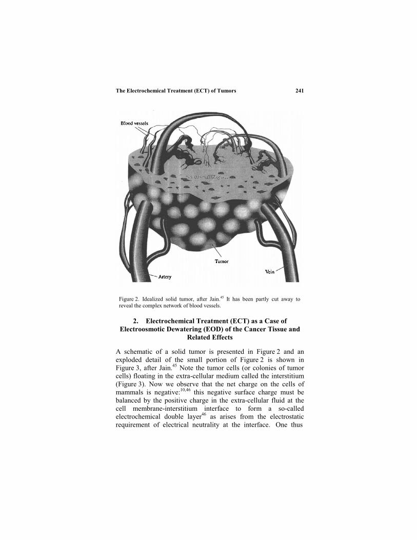
The Electrochemical Treatment (ECT) of Tumors 241
Figure 2. Idealized solid tumor, after Jain.45 It has been partly cut away toreveal the complex network of blood vessels.
2. Electrochemical Treatment (ECT) as a Case of
Electroosmotic Dewatering (EOD) of the Cancer Tissue and
Related Effects
A schematic of a solid tumor is presented in Figure 2 and anexploded detail of the small portion of Figure 2 is shown inFigure 3, after Jain.45 Note the tumor cells (or colonies of tumorcells) floating in the extra-cellular medium called the interstitium(Figure 3). Now we observe that the net charge on the cells ofmammals is negative:10,46 this negative surface charge must bebalanced by the positive charge in the extra-cellular fluid at thecell membrane-interstitium interface to form a so-calledelectrochemical double layer46 as arises from the electrostaticrequirement of electrical neutrality at the interface. One thus

Ashok K. Vijh2
Figure 3. A detailed depiction of a tiny section ( in Figure 1) of this tumor,
showing tumor cells, interstitium, a small blood vessel and the route that a drug in
the chemotherapeutic treatment takes. Adapted from Jain.45
arrives at a schematic description of negatively charged tumor(cancerous or normal) cells (or groups of cells) floating in theextra-cellular fluid creating surface electrical double layers andwith, between the cells (or colonies of cells), narrow intercellularfluid channels in the insterstitium (Figure 4). When a DC currentis passed between the two electrodes embedded in the tumor,electroosmotic flow of water occurs from the anode to thecathode, as described below.
The basic point here is that ECT causes a net flow of waterfrom the anode to the cathode, causing electroosmotic dewatering(EOD) of the tissue; the experimentally observed flow of waterfrom anodic site (dry) to the cathodic site (oedema) of the tumortissue can be explained only by an electroosmotic mechanism.
The EOD is based on the electrically-induced flow (viz.Electroosmosis) of water trapped between the tumor cells(Figure 4). Such electrically induced flow is possible because ofthe presence of electrochemical double layer at the cell-
Ashok K. Vijh242
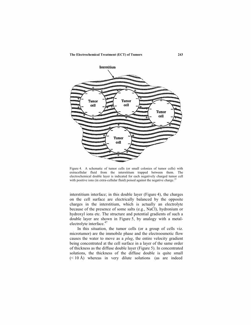
The Electrochemical Treatment (ECT) of Tumors 243
Figure 4. A schematic of tumor cells (or small colonies of tumor cells) withextracellular fluid from the interstitium trapped between them. Theelectrochemical double layer is indicated for each negatively charged tumor cellwith positive ions (in extra-cellular fluid) poised against the negative charge.25
interstitium interface; in this double layer (Figure 4), the chargeson the cell surface are electrically balanced by the oppositecharges in the interstitium, which is actually an electrolytebecause of the presence of some salts (e.g., NaCl), hydronium orhydroxyl ions etc. The structure and potential gradients of such adouble layer are shown in Figure 5, by analogy with a metal-electrolyte interface.47
In this situation, the tumor cells (or a group of cells viz.microtumor) are the immobile phase and the electroosmotic flowcauses the water to move as a plug, the entire velocity gradientbeing concentrated at the cell surface in a layer of the same orderof thickness as the diffuse double layer (Figure 5). In concentratedsolutions, the thickness of the diffuse double is quite small(< 10 Å) whereas in very dilute solutions (as are indeed
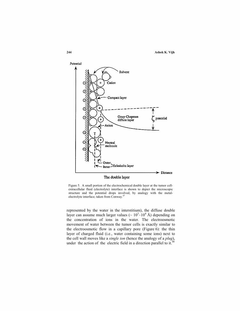
Ashok K. Vijh244
Figure 5. A small portion of the electrochemical double layer at the tumor cell-extracellular fluid (electrolyte) interface is shown to depict the microscopicstructure and the potential drops involved, by analogy with the metal-electrolyte interface; taken from Conway.47
represented by the water in the interstitium), the diffuse doublelayer can assume much larger values (~ 103–104 Å) depending onthe concentration of ions in the water. The electroosmoticmovement of water between the tumor cells is exactly similar tothe electroosmotic flow in a capillary pore (Figure 6): the thinlayer of charged fluid (i.e., water containing some ions) next tothe cell wall moves like a single ion (hence the analogy of a plug),under the action of the electric field in a direction parallel to it.48

The Electrochemical Treatment (ECT) of Tumors 245
Figure 6. A schematic of the electroosmotic flow of the medium (e.g., anelectrolyte) in a capillary caused by the flow of counter ions as a plug, under theinfluence of the applied electric field, E : Ueo is the convective liquid velocity fromelectroosmosis. Adapted from Everett.48
The origin of the electrochemical double layer arises from therequirements of charge neutrality in which the surface charge onthe cell surface must be balanced against the opposite charge inthe water (or any other fluid in a more general case).
Quantitatively, the convective liquid velocity fromelectroosmosis, Ueo, is given by the Helmholtz-Smoluchowskirelation:49, 50
EUeo (4)
where is the permittivity of the extracellular solution; is theviscosity of the extracellular solution; , is the so called zetapotential of the cell surface (see Figure 5); and E, is the appliedelectric strength, defined as the minus of the gradient of theelectrical potential (see Figure 6).
The potential is the potential difference between the planeof shear (or slipping plane) and the bulk solution. From Eq. (4), itis clear that for a given situation of water (electrolyte) in theinterstitium, the Ueo is proportional to the zeta potential and to theapplied field strength. Also in a real situation of EOD, it isnecessary to use the so called length-averaged value of the zetapotential in order to take into account the effect of the axiallyvariable zeta potential on the electroosmotic velocity.
Further, since both the zeta potential and the electric fielddepend on the ionic concentration and pH of the fluid (the tissue
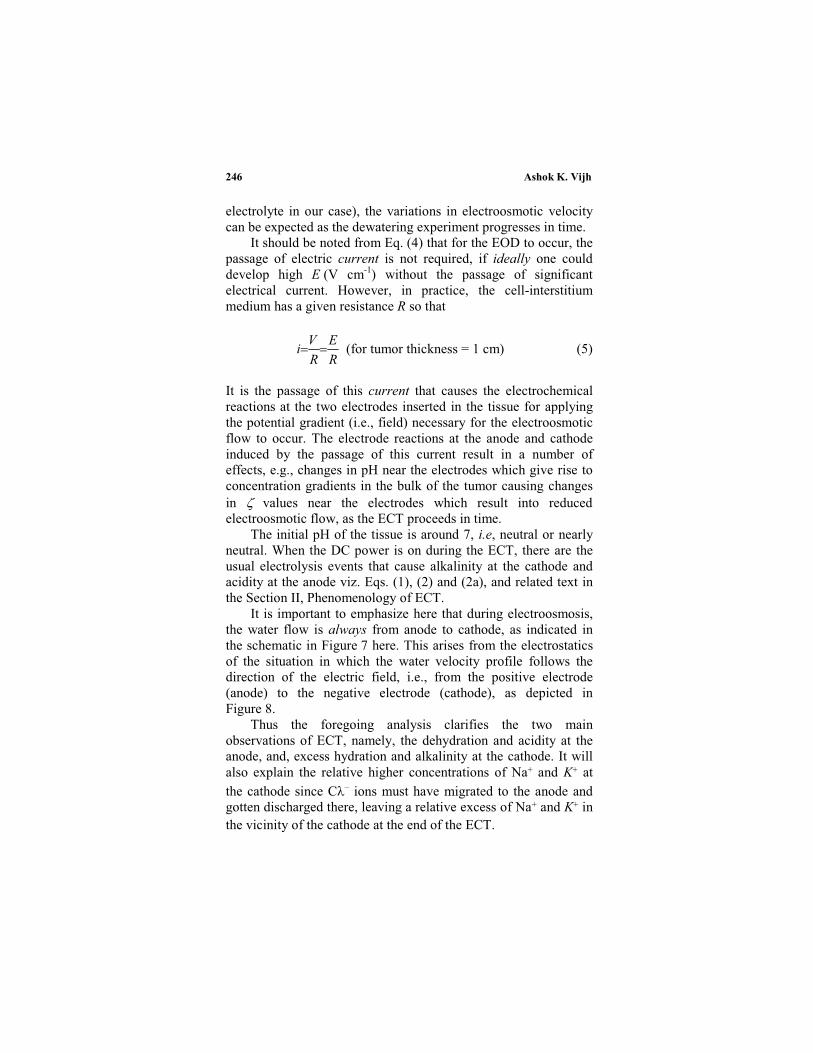
Ashok K. Vijh246
electrolyte in our case), the variations in electroosmotic velocitycan be expected as the dewatering experiment progresses in time.
It should be noted from Eq. (4) that for the EOD to occur, thepassage of electric current is not required, if ideally one coulddevelop high E (V cm-1) without the passage of significantelectrical current. However, in practice, the cell-interstitiummedium has a given resistance R so that
R
E
R
Vi (for tumor thickness = 1 cm) (5)
It is the passage of this current that causes the electrochemicalreactions at the two electrodes inserted in the tissue for applyingthe potential gradient (i.e., field) necessary for the electroosmoticflow to occur. The electrode reactions at the anode and cathodeinduced by the passage of this current result in a number ofeffects, e.g., changes in pH near the electrodes which give rise toconcentration gradients in the bulk of the tumor causing changesin values near the electrodes which result into reducedelectroosmotic flow, as the ECT proceeds in time.
The initial pH of the tissue is around 7, i.e, neutral or nearlyneutral. When the DC power is on during the ECT, there are theusual electrolysis events that cause alkalinity at the cathode andacidity at the anode viz. Eqs. (1), (2) and (2a), and related text inthe Section II, Phenomenology of ECT.
It is important to emphasize here that during electroosmosis,the water flow is always from anode to cathode, as indicated inthe schematic in Figure 7 here. This arises from the electrostaticsof the situation in which the water velocity profile follows thedirection of the electric field, i.e., from the positive electrode(anode) to the negative electrode (cathode), as depicted inFigure 8.
Thus the foregoing analysis clarifies the two mainobservations of ECT, namely, the dehydration and acidity at theanode, and, excess hydration and alkalinity at the cathode. It willalso explain the relative higher concentrations of Na+ and K+ at
the cathode since C – ions must have migrated to the anode andgotten discharged there, leaving a relative excess of Na+ and K+ inthe vicinity of the cathode at the end of the ECT.
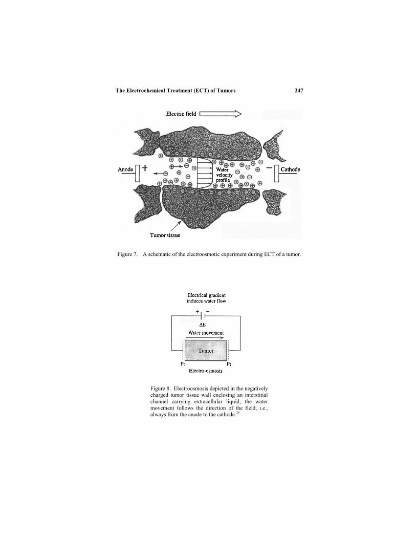
The Electrochemical Treatment (ECT) of Tumors 247
Figure 7. A schematic of the electroosmotic experiment during ECT of a tumor.
Figure 8. Electroosmosis depicted in the negativelycharged tumor tissue wall enclosing an interstitialchannel carrying extracellular liquid; the watermovement follows the direction of the field, i.e.,always from the anode to the cathode.25
Ashok K. Vijh248
3. Some Possible Factors in the Necrosis of Cancer Tumors
by ECT
The most important factor in tissue death during ECT appears tobe dehydration in the anode area and excess hydration (oedema)in the cathode area. This factor is reinforced by high acidity at theanode and excess alkalinity at the cathode. Hyperthermia wouldappear to be unimportant except perhaps towards the end of ECTexperiment when the anode area is quite dry and thence of highelectrical resistance and supports enhanced local heating.25
Oxidation by C 2 (or chloride radicals adsorbed at theplatinum electrode as Pt-C ), O2, O3 (which must be evolved intraces at the high anodic potentials attained in ECT carried out athigh current densities) at the anode are no doubt responsible fornecrosis in the tissue around the anode; one can even see visiblechanges such as bleaching and/or other colour changes. Aroundthe cathode, the erosive damage may be caused by cavitation bythe profusely evolving hydrogen. Also, hydrogen evolution wouldexpel any oxygen in the tissue around the cathode so thatrespiration by the tumor cells needed for their survival andgrowth would be inhibited, leading to their necrosis.
The traumatic changes brought by ECT would also tend tobreak and dismantle the hydrogen-bonding network of DNA ofthe tissue thus suggesting another mechanism for necrosis.25 Thefollowing other possible contributions to the necrosis of thecancer tumor during ECT may also be noted:
1. Micro-Thromboses: Platelets and leucocytes, like othercells, are known to carry surplus negative charge, and canbe electrophoretically deposited at (or around) the anode10
owing to the positive electrode potential. Thesemicrothromboses in capillaries in or near the treatment sitewill result in decreased blood flow and may contribute to alocal dystrophy of the tissue. A more pronounced versionof this effect can be seen sometimes as electrocoagulationand vascular occlusion (i.e., shut, closed or obstructedvasculature) of the tumor tissue. In other words, ECT cutsoff the blood supply to the tumor and causes the tumor cellnecrosis.
2. Reactive Oxygenated Species (ROS): Not only can reactiveradicals (arising from oxygen or chlorine evolution) be
The Electrochemical Treatment (ECT) of Tumors 249
produced at the anode, but reduction of any oxygenavailable around the cathode can give rise to H2O2 andperoxide damage of the cancer tissue;26 alternatively,hydrogen evolution at the cathode can cause hypoxia(oxygen deficiency) and tissue death. Since solid tumorsare hypoxic (oxygen deficient), cathodic reduction of O2 toproduce H2O2 etc. would not be an important reaction.
3. Other Factors: ECT no doubt destroys the homeostasis ofthe cancerous cells by profoundly disturbing their micro-environment and by dismantling their structure. It mightalso lead to the inhibition of their DNA synthesis. It hasbeen speculated that ECT might release the TumorNecrosis Factor (TNF) or, somehow super-activate theimmune system at the tumor site.
It has been suggested10,18 that the electroosmotic movementof water towards the cathode that causes oedema at the cathodesite leads to increase of tissue turgor pressure there:18 it results incompletely suspended circulation in the capillaries in the cathodicfield leading thus to tissue death.
4. Approaches to the Possible Improvement of the
Electrochemical Treatment (ECT) of Cancer Tumors
Based on considerations of fundamental electrochemistry, ideaswere presented in 1999 to improve the application of the ECTtechnique;25 to our knowledge, this approach has not been triedexperimentally. The argument involved is as follows:
By drawing analogy from the case of electroosmoticdewatering (EOD) of electrolyte trapped in the interstices betweenfine clay particles (cf. Figure 2 in which tumor cells are replacedby negatively-charged fine clay particles), one notes that electrodereactions at the anode and cathode cause pH changes that reducethe rate of water removal as the ECT proceeds; in other words theinitial potential (cf. Eq. 4) assumes lower values with time (dueto pH changes) as the ECT proceeds. In order to restore theoriginal potential value, one should gradually lower and thenstop the current and short-circuit (after disconnecting the powersource) the anode and cathode for a couple of minutes beforerestarting the ECT; this short-circuiting restores the original

Ashok K. Vijh250
potential and thence the high rates of dewatering observed at thecommencement of the process.49,50 Also, subsequent to the short-circuiting, a reversal of the direction of the current for a minute orso also achieves the same goal in a more enhanced manner; thislatter would then also have roots in the suggestion ofNordenström18 in which a reversal of the current in the tissues isachieved. In electrochemical terms, this restores the high potential (Eq. 4 here) and therefore causes the recommencementof EOD at high rates once the normal polarity of the ECT is re-established.
Other possible improvements in ECT are the suggestedbenefits of combining ECT with other established treatments suchas chemotherapy51 or radiotherapy;52 both these studies found thecombination therapy more effective. Also, immunologically-related compounds such as TNF- , IFN- and IL-2 wereobserved to enhance the effect of ECT when used in combinationwith the latter.53,55 The studies have also been covered in a recentsynoptic review.20 This combination therapy was also pioneered,it seems by Nordenström in Sweden;14,15 he also describes thedetails of the electrode wire electrodes, cannula and catheter etc.he used in his work.14
Another possible avenue for the understanding andimprovement of ECT is through mathematical modelling of theECT, as has been explored by Nilsson and coworkers.57,58 In onestudy,57 they concluded that during ECT, the direct current is nottransported homogeneously in the tissue but through thin channelsof institial fluid, which is consistent with the detailedelectroosmotic theory of ECT25 described in Section III.2 of thisChapter. In another investigation,58 Nilsson et al. carried outsimulations by modelling tissue as an aqueous solution of sodiumchloride containing a bicarbonate buffer system and organicconstituents susceptible to reactions with chlorine. Theyconcluded that in ECT at moderately high current densities, it isthe spreading of hydrogen ions—and not chlorine molecules—that determines the range of tissue destruction around the anode;this, again, is consistent with the observations of many workers59
and the facts that H3O+ migrates through the tissue much faster
than Cl2, and, large shifts in pH are observed during the ECT.25
Thus the tissue necrosis by chlorine-based species will be in the

The Electrochemical Treatment (ECT) of Tumors 251
immediate vicinity of the anode whereas tissue destruction by lowpH (i.e., H3O
+) will cover a much larger area around the anode.
5. In-Vitro Studies on the Suppression of Cell Proliferation
by the Passage of Electric Current
It is somewhat surprising that only a few investigations areavailable on the in-vitro studies of the suppression of cancer cellproliferation by the passage of electric current; almost allpublications deal with the in-vivo work on solid tumors.
Lyte and Coworkers60 examined the effect of low level DCcurrent on some mouse lymphoma cells; within a narrow currentrange (10–24 A), some inhibition of the cell proliferation wasobserved whereas an enhancement of cell proliferation was notedoutside this current window. The data60 thus appear somewhatcontradictory and, in any case, were not interpreted as due toelectrochemical effects although a vague relevance of this work toinvestigations of Nordenström10-18 was implied and anelectrochemical mechanism thus insinuated.
An in-vitro electrochemical treatment (ECT) of KB cellsfrom a human oropharyngeal carcinoma line has been carried outby Yen and coworkers;61 inhibition of cell growth in culture wasobserved and found to depend on the magnitude of current andtreatment time. Results were interpreted in terms of pH effectscaused by ECT.
In another detailed study,62 the target tumor cells for the DCtreatment were mouse mastocytoma P815. The current was passedin a three compartment cell in which the cathode compartment(CC) was separated from the anode compartment (AC) by theinsertion of an intermediary chamber (IC) which had neither theanode nor the cathode; the three compartments were connected inseries via filter-paper bridges (Figure 9). Each of the threecompartments contained 2 ml of cell suspension and 2 mA currentwas passed through platinum electrodes inserted in the AC andCC chambers (Figure 9). The salient results of this study are asfollows:
1. In the cathodic chamber, cell lysis and increase in pH wascaused by the ECT; however, when the cells were treatedin phosphate buffer—a stronger buffering system that doesnot allow pH variations as a consequence of DC

Ashok K. Vijh252
treatment—neither of these effects were observed. Thus inthe cathode chamber ECT causes increase in pH by theproduction of OH- (cf. Eq. 1 here) which in turn causes celllysis.
2. In the anodic compartment, ECT leads to greatlydiminished cell viability; however, if instead of ECT, thecells were incubated in a solution of the same pH as wasobtained in the anodic compartment after the passage ofcurrent, cell viability did not diminish. One may concludethat pH is not the main factor in the cell viability in theanodic compartment.
3. When the regular saline solution is replaced by a phosphatebuffer in the anode compartment (which means absence of
Figure 9. Schematic representation of the acrylic chambers used fortreatment of P815 cells with DC. Chambers are connected in series by filter-paper bridges, and fitted with platinum electrodes in their extremities. In thissystem, cell suspensions can be exposed directly to the anodic reactions(AC) or cathodic reactions (CC) or to electric current without contact withthe electrodes, in the intermediary chamber (IC). Internal volume: 3 cm3.After Veiga et al.62
The Electrochemical Treatment (ECT) of Tumors 253
chloride ions) ECT experiment does not diminish the cellviability. Hence the annihilation of cancer cells in theanode compartment during ECT is due to chlorineevolution and does not take place owing to pH change.
4. After the ECT, the cells in the intermediary chamber (IC inFigure 9) have the same cell viability as the untreated cells.This means that the effect of ECT arises from theelectrochemical reactions (cf. anode and cathodecompartments) and that its origin does not lie in purelyelectrical effects that may be associated with the passageof current or the presence of voltage drop and thence theelectrical field (cf. intermediary chamber).
5. It was observed62 that ECT induces changes (i.e., in theanodic and cathodic compartments) such as cell membranedamage, alterations in cell shape and chromatinorganisation, mitochondrial swelling and condensation,cytoplasmic swelling and matrix rarefication; in otherwords, profound and destructive changes in the cellularstructure and environment, as was also mentioned inSection II, Phenomenology of ECT of solid tumors.
6. An additional62 major alteration at the cell surface of P815cells subjected to ECT was disturbance and disruption ofcarbohydrate expression. Carbohydrate-mediatedinteractions are involved in the adhesion of cancer cells toendothelial cells, which is correlated with metastasis.63
These carbohydrate groups help negotiate the cell’srelationship to its external environment. Cancer cells speaka different sugar dialect than do the normal cells;64 if ECTwere to inhibit specific glycosylation reactions, asindicated,62 it might be able to alter these pathways andturn off the cancer cell. Hence, one possible way in whichECT can destroy the tumors is by modifying and/ordisrupting the carbohydrate groups on the surfaces ofcancer cells.
Ashok K. Vijh254
TUMORS IN ANIMALS
Although the ECT work was initiated on human beings1-6 in thenineteenth century, the more recent work involves in-vivo
investigations on a variety of model animals at least in theoccidental world; in parallel, there is considerable clinical work inChina,30-32 and to a lesser degree, in some other countries.18,28,34 Asurvey of some representative ECT studies on animals ispresented next.
1. Mice
Humphrey and Seal9 (U.S.A.) reported in 1959 detailedexperiments on the ECT of sarcoma-180 tumors in nearly500 mice. In a typical experiment, 18 test animals and 18 controlanimals were used; the ECT was done with 3 ma current, at 6 Vfor 3 hours a day, for 24 days. They observed that after such alengthy treatment, the mean volume of test tumors was about 15%of the mean tumor volume of the control group; seven miceshowed complete tumor regression as a result of ECT. Totalregression means that the tumor has decreased progressively involume, hardened, dropped off, leaving a new skin surface at theformer tumor site.
In some related experiments,9 they concluded that ECT didnot show any promise in the treatment of leukemia in miceinduced by intraperitoneal L1210 tumor tissue implant; in otherwords, ECT is useful for solid tumors only.
The work of Ito and coworkers65 (Japan) on fibrosarcoma inmice showed that ECT retarded the tumor growth in mice; thebest results were obtained when ECT was preceded by a radiationtreatment.
Morris et al.66 (U.S.A.) induced Lewis lung carcinoma (LLC)in C57 black mice and subjected them to ECT: constant current of20 mA (which gave rise to 8–10 V as the voltage across theelectrodes) was applied for 15 minutes. Animals treated with ECTsurvived longer and exhibited a small primary tumor burden atdeath as compared to the control group, although no completeregression of the tumor was observed. It would appear that a
IV. ELECTROCHEMICAL TREATMENT (ECT) OF

The Electrochemical Treatment (ECT) of Tumors 255
treatment time of 15 minutes was probably too short to kill thetumor.
Griffin and coworkers (U.K.) reported work on ECT ofmammary carcinoma in mice.67 Tumor destruction was found tobe significantly greater, for a given charge, when anode wasimplanted in the tumor with cathode outside it. The resultsdemonstrated a linear relationship between the volume of tumorregression induced and the quantity of electric charge passed.
A very active group in Slovenia involving Miklav i , Seršaand coworkers have done extensive work on the ECT of tumors inmice.68-72 The effect of direct current (0.2 1.8 mA) onfibrosarcoma and melanoma tumors in mice was examines for30–90 minutes, either in single dose or repetitive treatments.Several electrode materials were investigated, e.g., Pt, Pt-Ir, Au,Ag, Ti and stainless steel. A number of electrode configurationswere also explored, e.g., one electrode placed in the tumor and thecounter electrode in the healthy tissue, or, so called the field
configuration where both electrodes were placed in the healthytissue on opposite sides of the tumor. A decrease in the tumorvolume was noted with all electrode materials and configurations.The tumor growth retardation was proportional to the electricalcharge passed. The best ECT effect was achieved by using amulti-array electrode.69 The other interesting work of this group,mentioned in a previous Section,51-56 uses ECT in combinationwith bleomycin or immunomodulators such as tumor necrosisfactor (TNF- ), interferon- (IFN- ), interleukin-2 (IL-2) etc.,with much beneficial effects.
In the work of Cabrales and coworkers73 (Cuba), sixty maleBALBC mice were used and Ehrlich tumors were implanted inthem. When the tumor volumes reached 850 mm,3 four platinumelectrodes were inserted into each tumor: ECT was carried out at4 mA for 21 minutes, total charge thus passed through each tumorwas around 5 coulombs. Tumor volume decrease and necrosispercentage increase were significant in mice treated with ECT, incomparison with the control group without ECT.
It is clear that in these studies on the ECT of solid tumors inmice, an appreciable reduction in the tumor volume or itscomplete necrosis is generally observed.
Ashok K. Vijh256
2. Hamsters
In their work74 on the ECT of melanoma tumors in hamsters,Schauble et al. (U.S.A.) implanted a 1.5 V battery as the powersource. A stainless steel point electrode was placed in the tumor,either as anode or as cathode and a counter electrode made ofplane wire mesh was applied to the skin of the chest. Threedifferent current levels were used: 3 mA; 0.5 mA; 1 A. The twohigher currents produced necrosis of the tumor at the dose leve of1h/day for 4 consecutive days. A more pronounced effect wasobserved with anode in the tumor and cathode outside it.
David and coworkers (Canada) investigated the effect of ECTon amelanotic melanoma (T1-4) solid tumors in hamsters.75 Thetreatment consisted of a passage of currents from 0.1 to 2.4 mA,for 1h/day for five consecutive days. Treated tumors decreased inmass (as a percentage of controls) to 89% at 0.1 mA and to 2% at2.4 mA. Similar results were obtained with both stainless steeland platinum—30% iridium electrodes. It was observed that evenat the higher current level, a thin rim of viable cells still remainedaround the periphery after the treatment: it would thus appear thatthe treatment did not use high enough currents for sufficientlylong periods and the electrode configuration probably did not spanthe entire tumor during ETC.
3. Rats
Gardner et al.75 (U.S.A.) injected ascetic Walker sarcoma cellsinto male albino Wistar rats and thus induced tumors in their liver.These tumors were than subjected to ECT by using an implanted1.5 V mercury battery as the power source; platinum electrodeswere used. Although no mention was made of the level of currentpassed, it must be quite low based on the battery voltage and theresistors used in their circuit. In any case, they observed that a lotof cells clumped around the anode—they interpreted this as theattachment of negatively charged cancer cells to the positiveelectrode. Obviously, the ECT treatment was not strong and longenough to cause necrosis or tumor regression etc.
Habal77 (U.S.A.) used small direct current (0.4–0.6 A,10–24 days) drawn from an implanted power source in his ECT ofhepatoma tumors in rats. The power sources (1.5 V) were

The Electrochemical Treatment (ECT) of Tumors 257
implanted after different times following the tumor implants inrats; the tumor growth retardation only occurred when thetreatment was started at an early stage.
Samuelsson78 (Sweden) used ECT to destroy colonadenocarcinoma tumors in rats by applying 10–40 mA currentsfor 1 h and using one to three treatments. Torpedo shapedplatinum electrodes were used, with an anode inserted in thecentre of the tumor and a cathode placed at the tumor surface. Theresults obtained by ECT were comparable to those obtained bysurgery: 50% of the rats treated with either ECT or surgery weredevoid of tumors when killed 7 months after inoculations thatinduced the tumors.
In other study,79 Samuelsson and coworkers (Sweden)investigated the efficacy of either ECT or radiotherapy or acombination of the two in destroying experimental coloncarcinoma tumor in rats. The combined treatment resulted intumor growth inhibition, and, total regression was obtained in75% of the cases; with radiotherapy alone, 75% of the tumorsremained. As mentioned above78 with ECT alone, the regressionrate was 50%, the same as surgery alone.
In the work of Griffin and coworkers (U.K.) mentioned20 inSection I, Introduction and Origins, ECT was used in apre-clinical work on the normal livers of male adult outbreadwhite (OBW) rats: the objective here was to observe the patternsof necrosis induced preclinically in the liver itself since it will bethe primary normal tissue at risk in the proposed ECT therapy.ECT induced two distinct regions of necrosis, distinguishablehistologically and by magnetic resonance imaging: (i) acylindrical region of primary necrosis centred on the electrode, itsvolume directly proportional to the charge passed, but greater atthe anode than cathode; (ii) a wedge-shaped infarct, apex at theelectrode and base extending to the liver edge. The extent of thisinfarct was greater at the anode than the cathode but showed asigmoidal relationship to the charge passed during ECT. Resultsindicated pH changes at the electrodes as likely mediators oftissue injury.
In the work of Chou et al.22 (U.S.A.) on rats (and mice), ECT,when used in multi-treatments, showed necrosis and regression inall treated tumors; the best 6 months rat tumor cure rate was 75%whereas the best 3 months tumor cure rate in mice was 59.3%.

Ashok K. Vijh258
The tumors under study in this work22 were radiation inducedfibrosarcoma (RIF-1) mouse tumor, and, rat fibrosarcoma.
Some other work from the laboratory of Chou andcoworkers80 (U.S.A.) was on the ECT of breast cancer in rats. Ratbreast cancers were initiated by injecting 1 106 MTF-7 cells intothe right mammary gland fat pad of Fisher 344 female rats. Theextent of tumor regression was related to the coulombic dose usein ECT: tumor control rate is less than 40% in the 40C (coulomb)and 60C groups, and, more than 70% in the 80C and 100C groups.
Turler and coworkers81 (Germany) examined theeffectiveness of ECT, in colorectal metastases established inBDIX rats by injection of colon cancer cells under the livercapsule. The tumors thus induced in the liver were subjected tolow current level ECT applied via five platinum electrodes(Figure 10). Four different applications were used:
60C cm-3, anode at the centre;60C cm-3, cathode at the centre;80C cm-3, anode at the centre;80C cm-3, cathode at the centre;
Figure 10. Electrode arrangement during the electrochemical treatment (ECT)with low-level direct current: one platinum electrode is placed at the center of thetumor, four electrodes with opposite polarity are inserted at the border between thetumor and the surrounding liver tissue. Taken from Turler and coworkers.81

The Electrochemical Treatment (ECT) of Tumors 259
In the control group, five electrodes were placed withoutapplying any direct current.
Histological examination81 of the removed livers showedsignificant destruction of the metastases with localized necroses inall treatment groups: 37% had a complete response rate and 63% apartial response rate. The best results were obtained in the groupwith an anode at the centre and a current dose of 80 C cm-3. Therewere no significant necrosis in the control group, as expected.
Colorectal liver tumor deposits in a rat model have also beenstudied by Maddern and coworkers82 in Australia. Significanttumor ablation was achieved by ECT conducted by employingseveral electrode configurations. Tumor necrosis was morecomplete with electrodes placed on either side of the tumor thanwith both electrodes placed in the centre of the tumor. In anotherstudy83 on the ECT of liver tumors in rats reported by the samegroup, i.e., Maddern et al. in Australia, a significant correlationbetween the current dose and the volume of necrosis, for a givenelectrode separation, was observed. These workers have alsopublished detailed histological studies on the ECT of normal ratliver and the successful healing of the tissue following thetreatment: this work thus established that electrolysis is a safemethod for creating defined areas of liver necrosis that heal wellwith no associated mortality. Such pre-clinical studies are crucialfor proving the suitability of ECT for clinical investigations in theWesterns countries.
And, finally, a remarkable study from the same group is onthe feasibility of electrolytic ablation of tissue on a rat pancreas;85
it is worth mentioning that currently, there are no ablativetechniques to treat pancreatic cancer in clinical use and this is anaggressive disease with less than 20% of patients suitable for acurative surgical resection.
Ten healthy rats were studies in total. Eight rats were treatedwith variable doses of coulombs and two rats were used ascontrols. ECT in the rat pancreas produced local necrosis andappears safe and reproducible in the healthy rat tissue; the nextstep is to examine its feasibility in a pig model pancreas, beforeevaluating it clinically for pancreatic tumors.
Ashok K. Vijh260
4. Pigs, Rabbits and Dogs
Earlier work on the electrolytic destruction of tissue in pigs is dueto Samuelsson and Jönsson86 in Sweden. The work on pigs hasbeen done on healthy issues (not on cancer tumors) with an aim toestablish the nature of tissue destruction, and subsequent healing,caused by ECT. This kind of work on large animals such as pigs,rabbits and dogs etc. is regarded as essential in the occidentalcountries as a prelude to possible clinical trials on human beingssince the parametric confines, safety, toxicity, necrosis andhealing patterns etc. can be established on a relatively largemammal.
In the work of Samuelsson and Jönsson,86 thirty lungs from26 healthy young pigs, weighing 20 to 30 kg, were subjected toECT. In most experiments, 8–10 V and 50 to 70 mA were usedand platinum electrodes were employed. Both anodic and cathodicsites showed coagulation necrosis and thrombosis in the vesselswhen examined microscopically. The lesions healed with fibroticscarring.
In their previous work on the electrolytic destruction of lungtissue in rabbits, the same Swedish group87 carried outexperiments on 130 rabbits weighing between 1.5 and 3 kg.Electrolysis resulted in destruction of tissue both at the anode andthe cathode. The anodic lesion has a pH around 3 whereas the pHwas about 10 at the cathode. Thrombi could, again, be seen in thevessels within the lesions.
A systematic series of studies on the ECT of pig liver haveappeared from the Australian group of Maddern et al. Electrolysiswas investigated for generating areas of hepatic necrosis in the pigliver.88 The lesions healed with time and were associated withminimum morbidity. Further work on 21 pigs showed that duringECT of the liver tissue the electrolytic dose (in coulombs cm-3)correlated with the volume of liver necrosis.89 This group alsoestablished that in addition to the coulombic dose, pH could beused as a realtime monitor to predict more accurately the extent ofnecrosis.
The normal range (i.e., before ECT) of pH values was 6.5 –8.7. A pH of less than 6 (at the anode) or more than 9 (at thecathode) reflected total cellular necrosis in those areas.90 Toelucidate the possible complications that may arise during ECT in

The Electrochemical Treatment (ECT) of Tumors 261
the liver region close to a major vein, Maddern and coworkersconducted another study.91 Under ultrasound control, in six pigs,platinum electrodes were inserted into, or immediately adjacentto, an hepatic vein. As electrolytic dose of 100C was thenadministered and the evolution of the lesion was monitored usingultrasound. Gas bubbles were seen to enter the hepatic veins orinferior vena cava during treatment in five of the six animals.There were no major complications as a consequence and allanimals recovered and remained in a healthy state until they werekilled.
This work88-91 clearly demonstrates that predictable andreproducible necrosis is produced by electrolysis in the pig liver.The treatment causes little or no damage to immediately adjacentliver or major vascular structures.
A very thorough study on the effects of direct current on dogliver has been reported by Li et al.33 and their main findings havebeen summarized in the beginning of Section II, Phenomenologyof ECT. This work brought out clearly the salient features of ECTsuch as changes in pH at the anode and the cathode, dehydrationof the tissue at the anodic site and oedema at the cathodic site,and, the role of the electrode reactions etc.
It is worth mentioning again that the work reported on mice,hamsters and rats was done on induced tumors and was aimed atdestroying them; however, the in-vivo investigations published onpigs, rabbits and dogs were carried out in healthy tissues with aview to elucidate the mechanisms, safety, toxicity, parametriclimits and techniques etc. of ECT, before applying them to humanbeings.
V. ELECTROCHEMICAL TREATMENT (ECT) OF
TUMORS IN HUMAN BEINGS: CLINICAL STUDIES ON
PATIENTS
The earlier clinical studies of ECT in the nineteenth century1-6
clearly showed the considerable potential of this technique,although standarized protocols could not be established; ECT thusfaded away without being integrated into the practice of surgery.
The rediscovery of this technique in clinical practice can betraced to the work of Nordenström11 in Sweden, about a quarter of

Ashok K. Vijh262
a century ago. The adoption of ECT as a common surgical tool toeliminate solid tumors, both cancerous and benign, has occurredin China which, again, can be attributed to the work andinspiration of Nordenström who helped train the initial cadre ofChinese surgeons in the clinical applications of ECT. The leaderof this immense Chinese effort is Yu-Ling XIN29-33 of the China-Japan Friendship Hospital in Beijing, who was previouslyassociated wit the Department of Biomedical Engineering,Hauzhong University of Science and Technology, Hauzhong,China.
1. The New Era in ECT
During the 1950’s, Dr. Björn E.W. Nordenström, a Swedishradiologist and surgeon, became curious about the appearance ofstreaks, spikes and coronas that he saw in the X-ray images oflung tumors: many of his colleagues either saw nothing orattributed these phenomena to artefacts in the images. In 1965Nordenström began a scientific exploration of these effects. Aftermuch experimentation and analysis, he showed that the necroticcentre of the tumor produces a voltage difference between thecancer tumor and the surrounding tissue; this provides the drivingforce for the electroosmotic movement of water, changes inconcentration profiles of ionic components of the tissue, and, theelectrophoretic transport of various organic molecules, thusproducing detectable structural changes such as coronas, streaksand spikes etc. in the tissue: this is the basis of the so-calledBiologically Closed Electric Circuit pathways (BCEC systems)theory of Nordenström elaborated in his book10 in 1983, andmentioned earlier in this Chapter. The central point of this theoryis the presence of electric field profile within the tissue (arisingfrom the voltage difference between the tumor and thesurrounding tissue) and its electrochemical consequences viz.electroosmosis, electrophoresis, pH changes etc. The co-transportof charged species (ions and electrons) caused by the presence ofelectric field creates continuous electric currents within the humanbody which are moderated by the living system and participate inmaintaining equilibrium and healing. He further argued that byaugmenting the healing process associated with the naturallyoccurring BCEC systems in the human body, electrotherapeutic

The Electrochemical Treatment (ECT) of Tumors 263
techniques could be developed to treat a variety of diseasesincluding cancer. This led him, in the late 1970s, to treat primarylung cancers by applying current between two platinun wireelectrodes. The anode was inserted in the centre of the lung tumorand the cathode was approximately twice the tumor diameteraway from the anode; the applied voltage was 10 V (DC).Preliminary work on five patients was reported11 in 1978, and, inhis book published in 1983 he summarized the results on 26 lungtumors in 20 patients.10 Many of these patients were, for variousreasons (e.g., too old, too weak or too sick with other ailmentsetc), not suitable for conventional treatments such as surgery,radiation or chemotherapy. Regression was observed in 12 out of26 tumors and no signs of regrowth were detected after a 2–5 yearfollow-up period.
Further work14-15 from this group examined the combinedeffect of ECT and the chemotherapeutic agent, adriamycin. Byinjecting the electropositively charged adriamycin via the anodein the centre of the tumor, it could be dispersed, byelectrophoresis, uniformly into the surrounding tissue.Alternatively, adiramycin could be applied intravenously but itsconcentration could be augmented within the tumor by placing acathode within the centre of the tumor. These techniques wereapplied with beneficial results in a preliminary study of14 patients with large lung tumors, otherwise incurable.
Nordenström and his coworkers have also applied ECT tobreast cancer17 of a patient. Two years after the treatment,mammograms, taken at six-month intervals, could not detect anyremaining tumors.
Other Swedish work on the clinical applications of ECT isdue to Samuelsson and coworkers.92 By applying 80 mA for2–4 hours to five lung tumors in four patients, they achieved atumor reduction of 60–80%. Two to three platinum electrodeswere used in these experiments, all placed in the tumor.
2. Extensive Clinical Studies in China
In China, ETC has been tried on thousands of patients and theresults were summarized by Xin in 1994,30 1998,31 and 2002.32
Most of this work has been published in Chinese Journalsalthough a special issue of Eur. J. Surgery made this work
Ashok K. Vijh264
available in English in 1994. These investigations do not followthe occidental tradition of randomised and controlled clinicaltrials and the Western style characterization and follow-up rate ofpatients; also, the classification of the tumors is not alwayspresented in details. However, these observational studies30-32
make a compelling case that ECT provides a safe, effective andinexpensive way of treating solid tumors.
Approximately 11000 cancer patients with various kinds oftumors have been treated with electrochemical therapy (ECT).This immense task was accomplished by training 2300 medicaldoctors through more than 150 ECT training courses between1987–2001. There have been more than 1300 hospital and clinicsin China offering ECT treatment over the past fifteen years.Although most of the treated patients were Chinese, a number ofthem also came from Europe, Australia, U.S.A., and Japan.
Clinical experience in China32 indicates that tumor killingarea around an electrode is circular with a radius of 1 cm, so thatthe ideal distance between the anode and the cathode should beapproximately 2 cm. The output voltage from DC power sourcewas in the 6 V to 8 V range and the magnitude of current wasapproximately 60 mA to 80 mA. The electric quantity (totalcharge or dosage) for solid cancer tumors should be 80C to 100Cper 1 cm diameter (Note that some animal studies73, 81 propose theuse of similar coulombs per cm3 of the tumor volume).
Based on results on thousands of patients who underwentECT for a variety of tumors, Xin32 has published extensive data intabular from. Table 1 shows short-term (6 months) efficacy ofECT whereas Table 2 give the long-term cure rate of variouscancers treated with ECT. The results, it is claimed,32 are equal toor better than those obtained by other techniques, i.e., surgery,radiation and chemotherapy. It is further claimed32 that ECT canalso be applied to patients who cannot be treated by conventionaltechniques owing to their old age, general poor health, multipleailments or advances cancers.
The Chinese workers also obtained spectacular results(Table 3) in the treatment of benign tumors of serious nature.32 Inthe case of hemangioma (Table 3), a lower electric dosage of 30Cto 40C per cm of the tumor is recommended because this benigntumor is very rich in electrolytes and has a very high conductivity;higher coulombic dosages can cause local burns.

Ta
ble
1
Sh
ort-
Term
(6
Mo
nth
s) E
ffic
acy
of
EC
T.
Ob
jecti
ve R
em
issi
on
in
76
42
Ma
lig
na
nt
Tu
mo
rs
Trea
ted
wit
h E
CT
in C
hin
a,3
2 1
98
7–
200
1.
Res
po
nse
s w
ere
Det
erm
ined
by
Dir
ect
Mea
sure
men
t: C
R =
Co
mp
lete
Resp
on
se
PR
= P
art
ial
Res
po
nse
, N
C =
No
Ch
an
ges
, P
D =
Pro
gre
ssiv
e D
isea
se
CR
PRN
CPD
CR
+PR
Typ
eN
umbe
rof
cas
esN
o.%
No.
%N
o.%
No.
%N
o.%
Oes
opha
geal
can
cer
1595
348
21.8
766
48.0
319
20.0
162
10.2
1114
69.8
Lun
g ca
ncer
1113
412
37.0
445
40.0
155
13.9
101
9.1
857
77.0
Liv
er c
ance
r 9
6124
025
.042
744
.421
021
.9 8
4 8
.7 6
6769
.4Sk
in c
ance
r 9
5861
163
.834
736
.2
0
0
0
0 9
5810
0.0
Bre
ast c
ance
r 6
4418
028
.029
646
.0 6
4 9
.910
416
.1 4
7673
.9C
ance
r of
hea
d &
fac
e 5
9815
425
.828
046
.8 9
916
.5 6
510
.9 4
3472
.6
Met
asta
tic ly
mph
nod
e ca
ncer
361
135
37.4
145
40.2
57
15.8
24
6.6
280
77.6
Thy
roid
can
cer
250
89
35.6
110
44.0
36
14.4
15
6.0
199
79.6
Can
cer
of v
ulva
237
91
38.2
111
47.0
21
8.8
14
5.9
202
85.2
Mel
anom
a 2
27 7
934
.8 2
711
.9 2
711
.9 9
441
.4 1
0646
.7C
ance
r of
che
st a
ndab
dom
inal
wal
l 1
72 4
425
.5 8
147
.1 2
916
.9 1
810
.512
572
.6C
ance
r of
ora
l cav
ity
138
46
33.3
75
54.3
11
8.0
6
4.4
121
87.6
Rha
bdom
yosa
rcom
a 1
33 2
720
.3 4
936
.8 3
828
.6 1
914
.3
76
57.1
Paro
tid
canc
er
84
28
33.3
46
54.8
6
7.1
4
4.8
7
488
.1T
hroa
t can
cer
2
1
942
.9
942
.9
2 9
.5
1 4
.7
18
85.7
Pros
tate
can
cer
2
0
840
.0
735
.0
315
.0
210
.0
15
75.0
Oth
ers
130
39
30.0
51
39.2
20
15.4
2
15.4
9
069
.2
Su
m t
ota
l7
642
2540
33.2
3272
42.8
1097
14.4
733
9.6
5812
76.0
The Electrochemical Treatment (ECT) of Tumors 265

Ta
ble
2
Lo
ng
-Term
Eff
ecti
ven
ess
of
EC
T D
ete
rm
ined
as
the 1
–5
-Yea
rs
Su
rviv
al
Ra
te i
n 7
64
2 C
ase
s o
f M
ali
gn
an
t
Tu
mo
rs T
rea
ted
in
Ch
ina
,32 1
98
7–
20
01
1 ye
ar2
year
s3
year
s4
year
s5
year
sT
ype
Num
ber
of c
ases
No.
%N
o.%
No.
%N
o.%
No.
%O
esop
hage
al c
ance
r15
9512
85 8
0.6
969
60.
848
330
.323
314
.620
512
.9L
ung
canc
er11
1310
63 9
5.5
933
83.
874
667
.060
053
.943
238
.8L
iver
can
cer
961
771
80.
257
7 6
0.0
209
21.7
184
19.1
145
15.1
Skin
can
cer
958
958
100.
095
810
0.0
890
92.9
890
92.9
767
80.1
Bre
ast c
ance
r 6
44 6
18 9
6.0
568
88.
240
462
.740
462
.732
350
.2C
ance
r of
hea
d &
fac
e 5
98 5
01 8
3.8
428
71.
633
856
.532
754
.724
541
.0
Met
asta
tic ly
mph
nod
e ca
ncer
361
336
93.
129
5 8
1.7
258
71.5
184
51.0
139
38.5
Thy
roid
can
cer
250
242
96.
823
2 9
2.8
192
76.8
191
76.4
133
53.2
Can
cer
of v
ulva
237
223
94.
120
9 8
8.2
188
79.3
188
79.3
104
43.9
Mel
anom
a 2
27 1
94 8
5.5
157
69.
2 9
140
.1 1
9 8
.4
00
Can
cer
of c
hest
and
abdo
min
al w
all
172
140
81
.413
0 7
5.6
115
66.9
102
59.3
74
43.0
Can
cer
of o
ral c
avit
y 1
38 1
29 9
3.5
124
89.
911
180
.4 9
971
.7 8
561
.6
Rha
bdom
yosa
rcom
a 1
33 1
21 9
1.0
88
66.
2 5
138
.3
9 6
.8
00
Paro
tid
canc
er
84
7
8 9
2.9
76
90.
5 6
779
.8 5
970
.2 4
553
.6T
hroa
t can
cer
2
1
21
100.
0 2
110
0.0
19
90.4
17
81.0
14
66.7
Pros
tate
can
cer
2
0
20
100.
0 1
9 9
5.0
18
90.0
16
80.0
10
50.0
Oth
ers
130
124
95.
4 9
9 7
6.2
98
75.4
71
54.6
31
23.8
Su
m T
ota
l7
642
6824
89.3
5883
77.0
4278
56.0
3593
47.0
2752
36.0
Ashok K. Vijh266

The Electrochemical Treatment (ECT) of Tumors 267
Table 3
Long-Term Survival Rates of 1369 Cases of Benign Tumors
Treated by ECT in China,32
1987–2001
1 year 2 years 3 yearsType
Numberof cases No. % No. % No. %
Hemangiomaa 874 874 100.0 874 100.0 874 100.0Thyroid tumor 116 116 100.0 116 100.0 116 100.0Thyroid cyst 102 102 100.0 102 100.0 102 100.0Prostate
hypertrophyb 191 191 100.0 189 98.9 156 81.7Keloidc 86 86 100.0 86 100.0 86 100.0
Sum total 1369 1369 100.0 1367 99.8 1334 97.4a Hemangioma is a purplish or reddish benign tumor consisting of a network of
interconnecting capillaries.b Prostate hypertrophy is benign enlargement of the prostate.c Keloid is a thick scar resulting from excessive growth of fibrous tissue and
behaves as a benign tumor.
For lung cancer, some data comparing ECT with otherconventional techniques have been reported29 and are summarizedin Table 4.
Table 4
Long-Term (5 Years) Survival
Rates of Lung Cancer:
Comparison of ECT with other
Conventional Techniquesa
Technique % Survival at 5 yearsSurgery 42.5Chemotherapy 16.5Radiation and
chemotherapy 11.0ECT 25.5
a The above data are based on the review ofstudies reported by Xin et al.29 Note thatECT was conducted on patients who wereeither in advanced stages of lung cancerand/or had failed radiotherapy and/orchemotherapy.

Ashok K. Vijh268
3. Clinical Studies in Other Countries
As stated earlier, the clinical investigations in other countries arefew and far between since surgical practice treats ECT asexperimental therapy because protocols based on randomisedstudies are not established yet.
The Japanese work has been carried out by the group ofMatsushima28,93 in the Department of Surgery, Tokyo MedicalCollege. They found that a combination of ECT withchemotherapy gave the best results for treating patients with lungcancers; especially, the anti-cancer drugs tend to accumulatearound the electrodes when direct current is passed. In a clinicalstudy on 26 patients who received ECT either with or without theanti-cancer drugs, a decrease in tumor size was observed in morethan 70% the cases. In two cases, the use of ECT alone resulted incomplete regression of the tumors.28
Clinical work from Slovenia94 involves treatment of fivepatients with melanoma skin tumors; ECT was combined withsystemic chemo- and/or immunotherapy. Tumor mass reductionswere observed but no complete responses.
A very large study jointly conducted by investigators inFrance, U.S.A. and Slovenia, and, involving five cancer centreshas explored the effectiveness of electric current andchemotherapy combination in treating cutaneous andsubcutaneous malignant tumors.95
The current was applied in the form of electrical pulses inorder to permeabilize the membranes of the tumor cells for theentry of the chemotherapeutic agent bleomycin which is a verypotent cytotoxic molecule. Clinical complete responses wereachieved in 56.4% of the tumors and partial responses wereobserved in 28.9% of the tumors. This work is thus not strictlyelectrochemical treatment in the sense of Nordenström18 and Xin32
but is rather chemotherapy aided by electrochemical-drivenmovement of ions, molecules and drugs etc. (e.g., byelectroosmosis, electrophoresis) into the tissue regions targetedfor necrosis, as in several studies28,51,93,94 described earlier withinthis chapter.
The American partners in this large effort95 have reported,separately, on the novel electrode designs for administering thiselectrochemotherapy: electrical pulses permeabilize, or

The Electrochemical Treatment (ECT) of Tumors 269
electroporate, tumor cell membranes which allows thechemotherapeutic agent greater access to intracellular site ofaction and consistently provides improved responses relative totreatment with the drug alone.96 Other similar work from theU.S.A. may also be mentioned.97
In a joint study98 from the U.K. and Australia, metastaticcolorectal cancer lesions in the liver of a 58 year old man wereelectrolytically ablated. Follow-up CT scan suggested completetumor regression. The Australian team of Maddern andcoworkers99 performed ECT combined with surgery on ninepatients with hepatic deposits from colorectal carcinoma; withinthe electrolytically treated area, seven patients had no radiologicalevidence of recurrence at a median follow-up of 9 (range 6–43)months whereas local recurrence was detected in two patients. Sixof the nine patients had metastases elsewhere in the liver with fourhaving extrahepatic metastases. Three patients remain tumor free.Three patients died. The median survival was 17 (range 9–24)months from the time of treatment. A review article comparing
colorectal liver metastases has been jointly published by theU.K./Australian team.100 It was concluded that electrolysis offerspotential benefits over other techniques (e.g., cryotherapy,microwave coagulation therapy, radiofrequency ablation and lase-induced thermotherapy) that include the apparent ability to safelyand effectively treat lesions abutting major hepatic structures, and,lack of a systemic inflammatory reaction following electrolyticablation.
The salient points in the electrochemical treatment (ECT) oftumors, based on the detailed descriptions in this chapter, may besummarized as follows:
1. The approach involves a passage of direct electric currentthrough the tumor, thus destroying the diseased tissuethrough a number of electrochemical events.
2. As regards the mechanism of ECT, the passage of currentthrough the tumor gives hydrogen evolution at the cathodecausing cavitation (and hypoxia) of the tissue and chlorine
CONCLUSIONS
electrolysis with other local ablative treatments for non-resectable
VI.

Ashok K. Vijh270
evolution at the anode that results in bleaching anddestruction of the tissue in the anode area. Furthercontributions to the tissue necrosis are made by; (i) thechanges in pH caused by the electrode reactions; (ii)electroosmotic movement of water from the anode to thecathode causing dryness of the tissue in the anodic area andits oedema near the cathode area. All these eventsprofoundly perturb the metabolism of the cancerous tissueand destroy its structure and function, thus leading to theannihilation of the tumor. The passage of electric currentalso leads to micro-thromboses in the capillaries feedingthe tumor, reinforcing further the destruction of its tissue.
3. The methodology used is quite simple and empirical innature: an application of 6–10 volts (DC) between twoelectrodes about 1–2 cm apart within the tissue, causing apassage of 60–100 mA (with wire electrode area about0.2 cm2) and the experiment lasts from one to two hours. Ingeneral, an array of anodes and cathodes is used to coverthe entire solid tumor and the bordering tissue. A morerigorous and quantitative methodology is needed in orderto increase the efficacy and accuracy of ECT.
4. The ECT has been applied with much success both inanimals and human beings. It has been demonstrated to bea safe, effective and inexpensive procedure.
For it to be applied more extensively at the clinical level, oneneeds to develop standardized commercial instrumentation and itsutility has to be demonstrated in more controlled and rigorouspre-clinical and clinical studies in terms of the accepted surgicalnorms in North America and Western Europe.
REFERENCES
1J. Althaus, British Med. J. Nov. 15 (1875) 606.2F. H. Martin, J. Amer. Med. Ass. (JAMA) 8 (1886) 61; idem, ibid, 8 (1866) 85.3J. N. Freeman, J. Amer. Med. Ass. (JAMA) 8 (1886) 90.4Editorial, British Med. J. Dec. 6 (1873) 667.5E. Van de Warker, J. Amer. Med. Ass. (JAMA) 8 (1886) 88.6R. Newman, J. Amer. Med. Ass. (JAMA) 8 (1886) 88.7B. W. Watson, Med. Sci. Res. 19 (1991) 103.8N. Melczer and J. Kiss, Nature 4571 (1957) 1177.
The Electrochemical Treatment (ECT) of Tumors 271
9C. E. Humphrey and E. H. Seal, Science 130 (1959) 388.10B. E. W. Nordenström, Biologically-closed electric circuits, Nordic Medical
Publication, Stockholm, 1983.11B. E. W. Nordenström, IRCS Medical Science 6 (1978) 537.12B. E. W. Nordenström, Ann. Radiol. 28 (1985) 128.13B. E. W. Nordenström, Amer. J. Clin. Oncol (CCT) 12(6) (1989) 530.14B. E. W. Nordenström, Amer. J. Clin. Oncol (CCT) 13(1) (1990) 75.15S. Eksborg, B. E. W. Nordenström, and H. Beving, Amer. J. Clin. Oncol. (CCT)
13(2) (1990) 164.16H. Beving, S. Eksborg and B. E. W. Nordenström, Amer. J. Clin. Oncol (CCT)
13(2) (1990) 167.17E. Azavedo, G. Svane and B. E. W. Nordenström, Clinical Radiology 43 (1991)
84.18B. E. W. Nordenström, Eur. J. Surg, Suppl. 574 (1994) 93.19E. Nilsson, H. V. Eulor, J. Berendson, A. Thorne, P. Wersäll, I. Näslund, A-S.
Lagersted, K. Narfström, and J. M. Olsson, Biolectrochemistry 1 (2001) 1.20D. T. Griffin, N. F. J. Dodd, S. Zhao, B. R. Pullan, and J. V. Moore, British
J. Cancer 72 (1995) 31.21C. K. Chou, Bioelectromagnetics 18 (1997) 1.22C. K. Chou, J. A. Mcdougall, C. Ahn, and N. Vora, Bioelectromagnetics 18,
(1997) 14.23B. G. Fosh, J. G. Finch, M. Lea, C. Black, S. Wong, S. A. Wemyss-Holden, and
G. J. Maddern, British J. Surg. 89 (2002) 999.24P. S. Baxter, S. A. Wemyss-Holden, A. R. Dennison, and G. J. Maddern, Aust.
NZ. J. Surg. 68 (1998) 637.25A. K. Vijh, J. Mater Sci: Materials in Medicine 10 (1999) 419; A. K. Vijh,
Drying Tech. 17 (1999) 585.26S. Srinivasan, G. L. Cahan and G. E. Stoner, in Electrochemistry: The Past
Thirty Years and the Next Thirty Years, Chapter 4, Ed. by H. Bloom andF. Gutman, Plenum Press, New York, 1977.
27Eur. J. Surgery, Suppl. 574 (1994), the entire issue.28Y. Matsushima, E. Takahashi, K. Hagiwara, C. Konaka, H. Miura, H. Kato, and
Y. Koshiishi, Eur. J. Surg., Suppl. 574 (1994) 59.29Y. L. Xin, F. S. Xue, B. S. Ge., F. R. Zhao, B. Shi, and W. Zhang,
Bioelectromagnetics, 18 (1997) 8.30Y. L. Xin, Eur. J. Surg., Suppl. 574 (1994) 25.31Y. L. Xin, Preprints from the 2nd International Symposium on Electrochemical
Treatment of Cancer, Beijing, 27-30 Sept. 1998, p. 81-92.32Y. L. Xin, Journal of the IABC in Medicine and Biology, 1(1), (2002) 24. (Note:
IABC denotes International Association For Biologically-Closed ElectricCircuits (BCEC) in Medicine and Biology].
33K. H. Li, Y. L. Xin, Y. N. Gu, and B. L. Xu, J. Bioelectromagnetics, 18 (1997) 2.34C. K. Chou and R. L. Ren, in Complementary/Alternative Medicine—An
Evidence-Based Approach, Chapter 2, Ed. by J. W. Spencer and J. J. Jacobs,Mosby Publishers, Boston, 1999.
35Y. L. Xin, Eur. J. Surg., Suppl. 574 (1994) 31.36J. O’M Bockris (retired from Texas A & M University, College Station, Texas)
personal communication to A. K. Vijh (Sept. 3, 2000).

Ashok K. Vijh272
37N. L. Vora, Electrochemical Treatment of Breast Cancer with Direct Current,U.S. Army Medical Research and Material Command, Fort Detrick, Maryland21702-5012, U.S., Report on Award Number DAMD17-96-1-6184 (June 1999).
38S. L. David, D. R. Absolom, C. R. Smith, J. Gams and M. A. Herbert, CancerResearch 45 (1985) 5625.
39B. T. Mortensen and J. Bojsen, J. Biomed. Engg. 4 (1982) 100.40D. Miklav i , G. Serša, B. Kryžanowski, S. Novakovi , F. Bobanovi , R.
Golauh, and L. Vodovnik, Bioelectrochem. and Bioenergetics 30 (1993) 209.41D. Miklav i , G. Serša, S. Novakovi and S. Reberšek, J. Bioelectr. 9 (1990)
133.42M. B. Habal and M. K. Scauble, Surg. Forum 18 (1967) 88.43F. Shirazi and B. C. Towe, Proc. 8th BRAGS, Washington, D.C., Oct. 9-12,
(1988) p. 60.44M. P. Abbracchio, J. D. Heck, and M. Costa, Carcinogenesis 3 (1982) 175.45R. K. Jain, Sci. Amer. 271(1) (1994) 58.46S. Ohki, in Comprehensive Treatise of Electrochemistry, Vol. 10, Ed. by S.
Srinivasan, Y. A. Chizmadzhev, J. O’M Bockris, B. E. Conway, and E. Yeager,Plenum Press, New York,1985, pp. 188, 199.
47B. E. Conway, Theory and Principles of Electrodes Processes, Ronald Press,New York, 1965.
48D. H. Everett, Basic Principles of Colloid Science, The Royal Society ofChemistry, London, England, 1988.
49A. K. Vijh, Drying Technology—An International Journal 13 (1995) 215.50A. K. Vijh, in Modern Aspects of Electrochemistry, Ed. by J. O’M Bockris, B. E.
Conway, and R. E. White, Plenum Press, New York, 1999, Vol. 32, Chap. 4.51G. Serša, S. Novakovic, and D. Miklav i , Cancer Lett. 69 (1993) 81.52I. Ito and S. Hashimoto, Granto Kagaku Ryoho 16 (1989) 1405.53G. Serša, R. Golauh, and D. Miklav i , Anti-Cancer Drugs 5 (1994) 69.54G. Serša and D. Miklav i , Mol. Biother 2 (1990) 165.55G. Serša, D. Miklav i , Radiol. Oncol. 27 (1993) 280.56G. Serša, D. Miklav i , U. Batista, S. Novakovi , F. Bobanovi , and
L. Vodovnik, Anti-Cancer Drugs 3 (1992) 253.57E. Nilsson, J. Berendson, and E. Fontes, J. Electroanal. Chem. 460 (1999) 88.58E. Nilsson, J. Berendson, and E. Fontes, J. Appl. Electrochem. 30 (2000) 1321.59J. G. Finch, B. Fosh, A. Anthony, E. Slimani, M. Texler, D.P. Berry, A.R.
Dennison, and G. J. Maddern, Clinical Science 102 (2002) 389.60M. Lyte, J. E. Gannon, and G. D. O’Clock, Jr., J. Natl. Cancer Inst. 83 (1991)
116.61Y. Yen, J-R. Li, B-S. Zhou, F. Rojas, J. Yu, and C.K. Chou, Bioelectromagnetics
20 (1999) 34.62V. F. Veija, C. Holandino, M. L. Rodrigues, M. A. M. Capella, S. Menezes, and
C.S. Alviano, Bioelectomagnetics 21 (2000) 597.63G. Kannagi, Glycoconj. J. 14 (1997) 577.64J. Alper, Science 301 (2003) 159.65H. Ito, N. Shiegmatsu, T. Nakayama, I. Nishiguchi, Y. Ando and S. Hashimoto,
J. Jap. Soc. Cancer Therapy 23 (1988) 696.66D. N. Morris, A. A. Marino, and E. Gonzalez, J. Surgical Res. 53 (1992) 306.67D. T. Griffin, N. J. F. Dodd, J. V. Moore, B. R. Pullan, and J. V. Taylor, British
J. Cancer 69 (1994) 875.
The Electrochemical Treatment (ECT) of Tumors 273
68D. Miklav i , G. Serša, S. Novakovi , and S. Reberšek, J. Bioelectricity 9 (1990)133.
69D. Miklav i , L. Vodovnik, F. Bobanovi , S. Reberšek, G. Serša, S. Novakovi ,and R. Golouh, Electro-Magnetobiol. 11 (1992) 109.
70D. Miklav i , G. Serša, M. Kryžanowski, S. Novakovi , F. Bobanovi , R.Golouh, and L. Vodovnik, Bioelectrochem Bioenerg. 30 (1993) 209.
71G. Serša and D. Miklav i , Reg. Cancer Treat. 1 (1993) 31.72D. Miklav i , A. Fajgelj, and G. Serša, Bioelectrochem. Bioenerg. 35 (1994) 93.73L. B. Cabrales, H. C. Ciria, R. B. Bruzon, M. S. Quevedo, R. H. Aldana, L. B. de
Oca, M. F. Salas, and O. de la Guardia Peña, Bioelectromagnetics 22 (2001) 316.74M. K. Schauble, M. B. Habal, and H. D. Gullick, Arch. Pathol. Lab. Med. 101
(1977) 294.75S. L. David, D. R. Absolom, C. R. Smith, J. Gams, and M. A. Herbert, Cancer
Res. 45 (1985) 5625.76B. Gardner, A. Sterling, and J. Brown, Surgery 62 (1967) 361.77M. . Habal, J. Biomed. Mater. Res. 14 (1980) 789.78L. Samuelsson, Acta Radio. 22 (1981) 129.79L. Samuelsson, L. Jönsson, I-L. Lamm, C. J. Lindén, and S.B. Ewers, Acta
Radiol. 32 (1990) 1978.80R. L. Ren, N. Vora, F. Yang, J. Longmate, W. Wang, H. Sun , J-R. Li, L. Weiss,
C. Staud, J. A. McDougall, and C. K. Chou, Bioelectromagnetics 22 (2001) 205.81A. Turler, H. Shaefer, N. Schaefer, M. Wagner, D. Maintz, J.C. Qiao and A.H.
Hoelscher, Bioelectromagnetics 21 (2000) 395.82S. A Wemyss-Holden, G. S. M. Robertson, P. de la M. Hall, A. R. Dennison, and
G. J. Maddern, Digestive Diseases 18 (2000) 50.83G. S. M. Robertson, S. A. Wemyss-Holden, A. R. Dennison, P. de la M. Hall,
P. Baxter, and G. N. Maddern, British J. Surgery 85 (1998) 1212.84S. A. Wemyss-Holden, G. S. M. Robertson, A. R. Dennison, P. de la M. Hall, J.
C. Fothergill, B. Jones, and G. J. Maddern, J. Surg. Res. 93 (2000) 55.85B. G. Fosh, J. G. Finch, A. A. Anthony, M. Texler, and G. J. Maddern, BMC
Gastroenterology 1 (2001) 9.86L. Samuelsson and L. Jönsson, Acta Radiologica Diagnosis 22 (1981) 9.87L. Samuelsson, T. Olin and N. O. Berg, Acta Radiologica Diagnosis 21 (1980)
447.88S. A. Wemyss-Holden, G. S. M. Robertson, A. R. Dennison, P. S. Vanderzon, P.
de la M. Hall, and G. J. Maddern, Clinical Science 98 (2000) 561.89S. A. Wemyss-Holden, A. R. Dennison, G. J. Finch, P. de la M. Hall, and G. J.
Maddern, British J. Surgery 89 (2002) 579.90J. G. Finch, B. Fosh, A. Anthony, E. Slimani, M. Texler, D. P. Berry, A. R.
Dennison, and G. J. Maddern, Clinical Science 102 (2002) 389.91S. A. Wemyss-Holden, P. de la M. Hall, G. S. M. Robertson, A. R. Dennison, P.
A. Vanderzon, and G. J. Maddern, ANZ J. Surg. 70 (2000) 607.92L. Samuelsson, L. Jönsson, and E. Ståhl, Radiologe 23 (1983) 284.93Y. Matsushima, R. Amemiya, J-S. Liu, E. Tajika, H. Takakura, K. Oho, and Y.
Hayata, J. Jap. Soc. Cancer Ther. 24 (1989) 2341.94A. Plesni ca, G. Serša, L. Vodovnik, J. Jancar, L. Zaletel-Kragelj, and S.
Plesni ar, Eur. J. Surg. Suppl. 554 (1994) 45.95L. M. Mir, L. F. Glass, G. Serša, J. Teissié, C. Domenge, D. Miklav i , J. J.
Jaroszeski, S. Orlowski, D. S. Reintgen, Z. Rudolf, M. Belehradek, R. Gilbert,
Ashok K. Vijh274
M-P. Rols, J. Belehradek, J. M. Bachand, R. DeConti, B. Štabuc, M. emažar,P. Coninx, and R. Heller, British J. Surgery 77 (1998) 2336.
96R. A. Gilbert, N. J. Jaroszeski, and R. Heller, Biochmica and Biophysica Acta
1334 (1997) 9. 97S. B. Dev and G. A. Hofmann, Cancer Treatment Reviews 20 (1994) 105. 98D. P. Berry, A. R. Dennison, R. Ward, and G. J. Maddern, Dig. Surgery 17
(2000) 518. 99B. G. Fosh, J. G. Finch, M. Lea, C. Black, S. Wong, S. A. Wemyss-Holden, and
G. J. Maddern, Brisith J. Surgery 89 (2002) 999.100B. D. Teague, S. A. Wemyss-Holden, B. G. Fosh, A. R. Dennison, and G. J.
Maddern, ANZ J. Surg. 72 (2002) 137.

275
Index
AC impedance spectroscopy,
190
Active islands,
inactive electrodes, 213
Adsorption isotherms, 183
Analysis,
small-signal, 162
Anodic deposit formation, 145
Anodic processes,
formation of PS, 104
Aqueous polarization, 25
Array of anodes and cathodes,
270
Atomic force microscopy
(AFM), 175
Bockris, 42
Born equation, 46
Brownian movement, 39
Capillary condensation, 183
Cell metabolism, 235
Chandrasekhar, 43
Clinical applications,
ECT, 263
Continuous-flow stirred tank
electrochemical reactor,
152
Conway, 42
Copper dissolution,
anodic, 146
Corrosion,
fractal approach, 169
Cottrell behavior, 214
Cottrell equation, 185, 193
Coulostatic analysis, 162
Crystalline silicon,
anodic dissolution, 65
Current burst theory,
dissolution, 69
Current density,
porous silicon, 76
Current transient,
fractality, 197
Cyclic voltammetry, 189
DC treatment,
target tumor cells, 251
Deposit dissolution process, 145
Diffuse double layer, 244
Diffusion coefficients, 14
Dipole moments, 25
Discrete molecular models, 17,
22
Dissolution rate,
mass transfer, 68
Dissolution valence, 100
Dissolution valence,
effective, 75
Dissolution,
chemical, 75
Doped n-Si, 79
Doped p-Si, 79
ECT method,
standarized treatment, 237
Electric field,
human body, 262

276 Index
ionic concentration, 245
tumor, 262
Electrical current,
tumor treatment, 231
Electrical gradient,
water flow, 247
Electrochemical double layer,
cell interstitium interface, 243
charge neutrality, 245
Electrochemical engineering,
Markov theory, 136
Electrochemical processes,
non-diffusion-limited, 220
Electrochemical reactions,
dissolution of silicon, 103
Electrochemical techniques,
diffusion-limited, 169
Electrochemical treatment
(ECT),
of tumors, 232, 268
low-level direct current, 258
Electrochemical treatment,
salient points, 269
Electrode surface processes, 142
Electrodeposition,
fractal approach, 169
Electrolytic cell,
flow circulation, 160
Electrolyzer, 148
Electrolyzer,
parasitic reactions, 159
Electroosmosis,
interstitial channels, 240
Electroosmosis,
tissue, 240
Electroosmotic dewatering,
zeta potential, 249
Electroosmtic Dewatering
(EOD), 241
Electrophoretic transport,
organic molecules, 262
Electropolishing, 73
Electrostatic solvation free
energy,
qunatum-mechanical, 30
Erlang formula, 140, 143
Failed cells,
Markovian analysis, 153
First solvation shell, 2
Fowler, 42
Fractal dimension,
surface, 169
Fractal geometry,
Mandelbrot, 170
Fractals, self-similar, 171
nonrandom, 170
random, 170
self-affine, 169, 170
Free energies of solvation in,
11, 24
Free energies of solvation in
water, 23
Free energies, cavitation, van
der Waals, 33
Free energy perturbation
procedure (FEP), 20
Free energy,
hydration, 33
Fuel-cell electrocatalyst, 214
Fullerene,
solubility, 14
Gas adsorption, molecular probe
method, 181
General interaction properties
function (GIPF), 8
Gibbs free energy, 20
Gibbs-Helmholtz equation, 46
Growth rate, 76
Hartree-Fock calculations, 6
Hellmann-Feynman theorem, 1

Index 277
Helmholtz layer, 100
Helmholtz-Smoluchowski
relation, 245
HF solution, 120
Highest occupied molecular
orbital (HOMO), 54
Hildebrand,
solubility parameter, 51
Hirschfelder, 1
Hydration,
ionic enthalpies, 45
free energies, 45
Hydrogen
bonding, 10
evolution, 71, 235
evolution, cavitation, 269
Image analysis methods, 174
Interaction energies, 1
Interfaces, electrochemistry,
fractal approach, 167
Intramolecular interactions, 18
Ionic solvation,
continuum solvent models, 44
discrete molecular solvent
models, 43
Kolmogorov, 139
Langevin dipoles, 39
Laplace transforms, 187
Layer thickness, 143
Lennard-Jones potential, 17
Linear Sweep/Cyclic
Voltammetry, 188
Lithium transport,
cell-impedance-controlled,
220
Lowest unoccupied molecular
orbital (LUMO), 54
Mandelbrot,
fractal geometry, 167
Markov matrix, 138
Markov process, 136, 139
Markov chains, processes, 135
Mass fractal, 169
Mathematical modelling, ECT,
250
Mechanistic aspects,
electrochemical treatment,
240
Mesoporous carbons, 219
Metallic electrodes,
tumor destruction, 239
Models of solvent,
hybrid/intermediate, 38
Molecular dynamics, 2
electrostatic potential, 3
volume, 53
Monte Carlo simulations,
of solutions, 2
Multi-array electrode,
ECT effect, 255
Nernst equation, redox couples,
188
Nitroaromatics, 13
Nonpolar solvents, 11
Ohmic resistance, substrate, 107
Onsager, 28
Organic solutions, anhydrous,
103
Oxide film thickness, 114
Para-dinitrobenzene, 7
Partition coefficients, 12
Peak-current method, 189
Performance, Markovian
modeling, 148
Perimeter-area method, 178
Perturbation theory, 2
Phenomenology of ECT, 246
Photo holes, 119
Physical adsorption, 1
Poisson distribution, 140

278 Index
Polarization, solute molecule,
31
Pore
arrays, 85
branching, 89
diameter, 82
diameter, distribution of, 87
diameter, interpore spacing,
86
orientation, 87
Porous electrode, 218
Porous silicon, 71
formation, 71
morphological characteristics
of, 97
morphology, 65
Positive charge,
extra-cellular fluid, 241
Potential gradients,
double layer, 243
Potential,
effect of current and HF
Concentration, 83
Potentiostatic current transient
method, 185
Probability distribution, 157
Pt/polished Al2O3 electrode, 201
Randles-Sevcik equation, 188
Random walk, Ion, 142
Reaction field, 27
Reaction kinetics,
anodic, 98
Rough surfaces,
fractal geometry, 167
Roughness parameter, 174
Scanning electron microscopy
(SEM),
transmission electron
microscopy, 174
Scanninng tunneling
microscopy (STM), 174
Self-Affine fractal, 172
Silicon, 91
Silicon oxide,
dissolution, 112
Silicon substrate, 74
Silicon/Electrolyte interface, 99
Solute Hammiltonian, 25
Solvent effects, 15
Solvent,
continuum models, 26
Solvent-solvent interactions, 51
Space charge layer,
semiconductor, 106
Sputter-deposited Pt films, 204
Sputter-deposited, Pt film
electrodes, 201
Structure-activity relationships,
12
Supercritical solvents,
solubility in, 15
Surface fractal dimension,
interfaces, 174
Surface lattice structure,
silicon, 110
Surface tension, solvent, 33
Switching-Circuit operations,
analysis of, 157
Symmetry-adapted perturbation
theory (SAPT), 2
Tank electrolyzer, 150
TEM image analysis method,
218
Thermal emission,
of holes, 73
Solid tumor, 270
Solute-solvent interactions, 1, 9

Index 279
Transition layer, 92
Triangulation method,
fractals, 175
Zener tunnelling, 73
Zeta potential,
electroosmotic velocity, 245