Vaughan, F., Linden, N., & Manby, F. (2017). How Markovian is excitondynamics in purple bacteria? Journal of Chemical Physics, 146(12),[124113]. DOI: 10.1063/1.4978568

Publisher's PDF, also known as Version of record

License (if available):CC BY

Link to published version (if available): 10.1063/1.4978568

Link to publication record in Explore Bristol ResearchPDF-document

This is the final published version of the article (version of record). It first appeared online via AIP athttps://doi.org/10.1063/1.4978568 . Please refer to any applicable terms of use of the publisher.

University of Bristol - Explore Bristol ResearchGeneral rights

This document is made available in accordance with publisher policies. Please cite only the publishedversion using the reference above. Full terms of use are available:http://www.bristol.ac.uk/pure/about/ebr-terms.html

How Markovian is exciton dynamics in purple bacteria?Felix Vaughan, Noah Linden, and Frederick R. Manby

Citation: The Journal of Chemical Physics 146, 124113 (2017); doi: 10.1063/1.4978568View online: http://dx.doi.org/10.1063/1.4978568View Table of Contents: http://aip.scitation.org/toc/jcp/146/12Published by the American Institute of Physics

Articles you may be interested inAnnouncement: Top reviewers for The Journal of Chemical Physics 2016The Journal of Chemical Physics 146, 100201100201 (2017); 10.1063/1.4978399

Perspective: Found in translation: Quantum chemical tools for grasping non-covalent interactionsThe Journal of Chemical Physics 146, 120901120901 (2017); 10.1063/1.4978951

A multilayer multiconfiguration time-dependent Hartree simulation of the reaction-coordinate spin-bosonmodel employing an interaction pictureThe Journal of Chemical Physics 146, 124112124112 (2017); 10.1063/1.4978901

A new efficient method for the calculation of interior eigenpairs and its application to vibrational structureproblemsThe Journal of Chemical Physics 146, 124101124101 (2017); 10.1063/1.4978581

Effect of high-frequency modes on singlet fission dynamicsThe Journal of Chemical Physics 146, 044101044101 (2017); 10.1063/1.4973981

Convergence of high order perturbative expansions in open system quantum dynamicsThe Journal of Chemical Physics 146, 064102064102 (2017); 10.1063/1.4974926

THE JOURNAL OF CHEMICAL PHYSICS 146, 124113 (2017)

How Markovian is exciton dynamics in purple bacteria?Felix Vaughan,1,2 Noah Linden,3,a) and Frederick R. Manby1,b)1Centre for Computational Chemistry, School of Chemistry, University of Bristol, Bristol BS8 1TS,United Kingdom2Bristol Centre for Complexity Sciences, University of Bristol, 1–9 Old Park Hill, Bristol BS2 8BB,United Kingdom3School of Mathematics, University of Bristol, Bristol BS8 1TW, United Kingdom

(Received 28 September 2016; accepted 1 March 2017; published online 27 March 2017)

We investigate the extent to which the dynamics of excitons in the light-harvesting complex LH2of purple bacteria can be described using a Markovian approximation. To analyse the degree ofnon-Markovianity in these systems, we introduce a measure based on fitting Lindblad dynamics,as well as employing a recently introduced trace-distance measure. We apply these measures to achromophore-dimer model of exciton dynamics and use the hierarchical equation-of-motion methodto take into account the broad, low-frequency phonon bath. With a smooth phonon bath, small amountsof non-Markovianity are present according to the trace-distance measure, but the dynamics is poorlydescribed by a Lindblad master equation unless the excitonic dimer coupling strength is modified.Inclusion of underdamped, high-frequency modes leads to significant deviations from Markovianevolution in both measures. In particular, we find that modes that are nearly resonant with gaps in theexcitonic spectrum produce dynamics that deviate most strongly from the Lindblad approximation,despite the trace distance measuring larger amounts of non-Markovianity for higher frequency modes.Overall we find that the detailed structure in the high-frequency region of the spectral density has asignificant impact on the nature of the dynamics of excitons. © 2017 Author(s). All article content,except where otherwise noted, is licensed under a Creative Commons Attribution (CC BY) license(http://creativecommons.org/licenses/by/4.0/). [http://dx.doi.org/10.1063/1.4978568]

I. INTRODUCTION

Photosynthesis provides the energy for nearly all life onEarth. The conversion of light energy into biologically usefulchemical energy is a complex process performed by a varietyof different organisms. Energy is captured in the form of pho-tons and transported to a reaction center, where it is convertedinto useful chemical energy. The capture and transport process,generically known as light harvesting, is of great interest dueto its near unit quantum efficiency1,2 and because of recentsuggestions of long-lasting quantum coherent effects basedon two-dimensional (2D) femtosecond spectroscopic experi-ments.3–8 Understanding how light harvesting achieves suchhigh efficiency, and the role of quantum coherence in this effi-ciency, has been the goal of much theoretical and experimentalwork in the past few years, with heavy focus on the interactionof the excited states with their surrounding environment.

Within the body of theoretical work, many interestingand general insights into the potential role of the environ-ment have been gained through the use of the Lindblad masterequation.9–21 Ideas such as noise-assisted transport,9,10,12–14,16

quantum locking, and momentum rejuvenation14 have beenused to suggest how interactions with the environment canhelp speed up energy transport in networks of chromophores.

a)n.linden@bristol.ac.ukb)fred.manby@bristol.ac.uk

However, it is still not certain whether these phenomena playa role in the real biological context, where the assumptionsinherent in the master-equation approach may not apply. It hasbeen shown, for physically realistic values of the environmentcoupling, that Lindblad and the related Redfield equations failto capture the correct exciton-transfer rates.22

The question we address here is whether or not a prioriLindblad equations, parameterised in any manner, are capa-ble of reproducing the dynamics of exciton transfer. Previousresearch into this question has resulted in differing conclu-sions.23–26 In particular, within a dimer extracted from theFenna-Matthews-Olson (FMO) complex, small amounts ofnon-Markovianity were observed for an overdamped Brown-ian spectral density;23 however, in calculations using the quasi-adiabatic path-integral approach (QUAPI) on the full FMOcomplex with realistic spectral densities, no non-Markovianitywas found.24 Here we look at the degree of non-Markovianityin a dimer parameterised to reflect the B850 ring of lightharvesting complex two.

The role of underdamped intra-molecular modes hasbeen the focus of much attention recently, and in particu-lar modes that are resonant with energy gaps between exci-tonic eigenstates.11,27–33 In some pigment-protein complexes,these modes show significant coupling to the excitons.34–37

This has led to theoretical studies that provide evidence forthe important role they may play in assisting energy trans-port and in producing the long-lived coherences seen in 2Dspectroscopy experiments.27–33 The phenomenon whereby

0021-9606/2017/146(12)/124113/13 146, 124113-1 © Author(s) 2017

124113-2 Vaughan, Linden, and Manby J. Chem. Phys. 146, 124113 (2017)

these underdamped molecular vibrations induce long-livedcoherences and drive transitions between excitonic eigenstateshas been demonstrated using a semi-classical treatment ofthe intra-molecular mode,28 which it was claimed demon-strates that the fundamental mechanism is not dependent uponnon-Markovian dynamics. However, in Ref. 32 it is arguedthat, in models of dimers relevant for photosynthetic systems,efficient transport can show, and benefit from, non-classicaleffects, so there may be a significant role for non-Markovianeffects. The extent to which non-Markovianity is increasedthrough coupling to resonant modes is investigated in thispaper.

Much progress has been made in developing metrics forquantifying non-Markovianity in the dynamics of open quan-tum systems. For a thorough review of these measures, werefer the reader to Ref. 38. Broadly speaking these measurescan be categorised into those that look at properties of thedynamical maps that induce the time evolution of the sys-tem;39–43 monotonicity of distance measures between twotime-evolved trajectories of the system;44–47 and propertiesquantifying the correlations between the system of interestand an ancillary system.40,48–50 Other measures are basedupon the sign of decay rates of a Lindblad master equationin its canonical form51 and properties of the affine transforminduced by the dynamical map.52 Some of these measures arecomplete in the sense that they capture any deviation awayfrom the Markovian regime, whilst others capture only par-ticular aspects of non-Markovianity. The complete measureseither require information on the dynamical map or the useof an ancillary system which incurs extra, often impractical,computational cost. To tackle this issue we have developed ameasure of non-Markovianity based upon finding the closestfitting Lindblad master equation. This measure has the bene-fits of being bounded (between 0 and 1), and being related ina direct and straightforward way to the feasibility of using theLindblad approximation.

This paper is structured as follows: In Section II we dis-cuss the measures we will use to quantify the degree of non-Markovianity, introducing our measure based upon completeparameterisation and fitting of a Lindblad operator. In Secs. III,IV, and V, we apply these measures to chromophore dimersparameterised to model those of the light-harvesting complexLH2. In Section III we look at the effect of a broad phononbath on the degree of non-Markovianity, which we modelwith the hierarchical equations-of-motion (HEOM) method.We show that despite small amounts of non-Markovianity,the dynamics is well-captured by a Lindblad approach, pro-vided the site coupling in the excitonic Hamiltonian is a freeparameter. In Section IV we treat the same dimer system cou-pled to high frequency intra-molecular modes. We presentour calculations of the couplings to these modes which werecomputed using density functional theory calculations of abacteriochlorophyll-a (BChl-a) molecule. We investigate howthe degree of non-Markovianity varies with the number of dis-crete modes as well as the frequency of the discrete modes.We find that the degree of non-Markovianity increases withthe number of discrete modes for both measures of non-Markovianity. We also find that, according to the Lindblad fit-ting measure, vibrational modes resonant with the gap between

the excitonic eigenstates induce the most non-Markovianity.Finally, in Section V we combine both models and investigatemore realistic structured spectral densities using HEOM tomodel the phonon bath and include a discrete intra-molecularmode. Here we find that the discrete vibrational modes con-tribute significantly to the degree of non-Markovianity, callinginto question the use of Lindblad evolution to model excitondynamics.

II. THEORYA. Measuring non-Markovianity

Before exploring measures of non-Markovianity, it isworth considering a definition for Markovian dynamics intro-duced in Ref. 38. Let ρ(t) be the density matrix describing thedynamical evolution of the state of some quantum system. Thedynamical evolution from a state ρ(t1) to a state ρ(t2) at timest2 ≥ t1 can be described by the dynamical map that inducesthe evolution, Et2,t1 ρ(t1) = ρ(t2), where E is a completely posi-tive and trace-preserving (CPTP) map and does not depend onthe state upon which it acts. A family of such linear quantummaps Et2,t1 induces Markovian dynamics if for all t2 ≥ t1 ≥ t0it fulfills the composition law

Et2,t0 = Et2,t1Et1,t0 . (1)

Breuer et al.47 introduced a convenient measure for non-Markovianity based on the trace-distance metric. The tracedistance quantifies the difference between two states, ρ1 andρ2, and is defined as

D(ρ1, ρ2) =12

Tr |ρ1 − ρ2 | . (2)

It satisfies 0 ≤ D ≤ 1, and D = 0 if and only if ρ1 = ρ2, and D= 1 if and only if ρ1 is orthogonal to ρ2 (defined as Trρ†1ρ2 = 0).This metric has the property that it is a contraction under aCPTP map E,

12

Tr |Eρ1 − Eρ2 | ≤12

Tr |ρ1 − ρ2 | . (3)

From our definition of Markovian dynamics above, a Marko-vian evolution is induced by a CPTP map and due to thecomposition law in Eq. (1), any possible division of that evo-lution into smaller time steps is also a CPTP map. Thus thetrace distance between two initial states undergoing Markoviandynamics will monotonically decrease and any increase in thetrace distance indicates non-Markovian effects. This mono-tonic decrease can be intuitively understood as arising fromthe entirely dissipative nature of the bath in the Markovianregime. Both initial states continuously lose information to theenvironment as they tend towards the same steady state. Onlywhen there is a back-flow of information from the environ-ment can this process be temporarily reversed and the distancebetween the states be increased.

We would like to construct a measure for this propertyand quantify an answer to the question: given some dynami-cal process that takes ρ(0) → ρ(t), how non-Markovian is it?From the above property, Breuer, Laine, and Piilo (BLP)47 con-cluded that the degree of non-Markovianity can be quantified

124113-3 Vaughan, Linden, and Manby J. Chem. Phys. 146, 124113 (2017)

by calculating the extent to which the trace distance increasesbetween two density matrices starting at different initial states,

NBLP(ρ1, ρ2) =∫

dD(ρ1(t), ρ2(t))dt

θ

(dD(ρ1(t), ρ2(t))

dt

)dt,

(4)

where θ, the Heaviside function, ensures that the derivativeonly contributes to the integral when it is positive. This quan-tification is dependent upon the pair of initial states chosen.To remove this dependence, a search over all possible pairs ofinitial states can be performed and the maximum defined torepresent the degree of non-Markovianity for the system,

NBLP = maxρ1,ρ2

NBLP(ρ1, ρ2). (5)

The computational difficulty of performing such a maximisa-tion can be reduced by taking into account recently provedconditions for initial-state pairs that maximise NBLP,53 whichstate that the maximum occurs for initial states that areorthogonal and lie on the boundary of the state space (whichis equivalent to having a zero eigenvalue). An alternativeapproach is to consider typical initial states of the system.For the case of light harvesting, the true nature of the ini-tial state is still debated;26 however, for simplicity it is oftenassumed that the exciton is initially localised at a single chro-mophore. Thus, as well as looking at NBLP, we also inves-tigate the typical amount of non-Markovianity, based on thefully localised initial states for a dimer system. We note thatin such cases the degree of non-Markovianity may be anunderestimate.

We will refer to this measure as the BLP measure ofnon-Markovianity and, in order to distinguish it from otheruses of the trace distance in this paper, we will refer to thetrace distance calculation associated with it as the BLP tracedistance.

Although very useful, the disadvantages of the BLPmeasure are two-fold. First, there are some forms of non-Markovianity that the BLP measure will not capture.38,51,54

In particular, we write a state ρ of dimension d in the form

ρ =Id

+∑

i

αi Fi, (6)

where αi are the elements of a real d2� 1 dimensional vector

α known as the Bloch vector and F i are a set of orthogonaltraceless hermitian operators (e.g., the Pauli matrices for d = 2).The action of any dynamical map on ρ can now be written inthe form of an affine transform of the Bloch vector,

α(t) = Mα(0) + t. (7)

It may be shown that the trace distance between two evolvingstates is independent of the vector t.54 For this reason the BLPmetric is sometimes called a witness rather than a measure ofnon-Markovianity.38 Second, since the measure is not boundedabove, it is not clear for what values of the measure it can beconcluded that Lindblad-type master equations are no longer agood approximation. It is this second point that motivates theintroduction of a Lindblad fitting scheme.

Any quantum mapL inducing a Markovian time evolutioncan be written in Gorini-Kossakowski-Sudarshan-Lindbladform,38

dρdt= LL(ρ) =

i~

[ρ, H] + L(ρ), (8)

where the second term

L(ρ) =12

∑jk

hjk

(2Lj ρL†k − ρL†k Lj − L†k Lj ρ

)(9)

describes the dissipative effect induced upon the dynamics ofthe system by a Markovian bath, and where the Lj form acomplete set of orthogonal traceless operators and h is a posi-tive matrix. For a two-dimensional system, one can representthe density matrix ρ in its Bloch vector form (see Eq. (6)),ρ = I/2 +

∑3i=1 αiLi. The action of a Lindblad operator can

now be written as the affine transformation in Eq. (7).It can be shown that for a two-dimensional system that M

is a real symmetric matrix55 and can therefore always be diag-onalised. It is convenient to parameterise the eigenvalues of Mwith three real parameters qi such that the eigenvalues are �(q2

+ q3)/2, �(q1 + q3)/2, and �(q1 + q2)/2. The conditions on theparameters can be derived by ensuring that the correspondingmatrix h in Eq. (9) is always positive.56,57 These result in theconditions,

ti, qi ∈ R, (10a)

qi ≥ 0, (10b)

t21

q2q3+

t22

q1q3+

t23

q1q2≤ 1. (10c)

We then explore the complete set of Lindblad dissipators byvarying qi, ti, and the 3 × 3 orthogonal matrices (parame-terised by three real parameters β1, β2, β3 corresponding toangles) that diagonalise a general 3 × 3 symmetric matrix M.It should be noted that this parameterisation characterises fullyonly those Lindblad evolutions with constant rates. This simpleparameterisation, consisting of nine real parameters, makes itpossible to perform an optimisation to find the Lindblad masterequation that best fits a given quantum evolution.

Given some quantum evolution of a two-state system ρ(t),we can find the closest-fitting Lindblad evolution ρL(t) byminimising the function,

Q =1T

∫ T

0dt

12

Tr |ρL(t) − ρ(t)| (11)

with respect to the parameters ti, qi, and βi and subject tothe constraints in Eq. (10). In Eq. (11) we have employed thetrace distance to quantify the difference between the exactevolution and the Lindblad evolution at each time, t. Theintegral quantifies the total difference during the trajectory,resulting in Q being the mean trace distance between the twotrajectories. This measure acts as a complementary measureof non-Markovianity to the BLP measure presented earlier. Ithas the advantages that it is bounded between 0 and 1 and thatit directly quantifies the extent to which the non-Markovianitypresent in the system renders the Lindblad master equationineffective at capturing the dynamics. Examination of the prop-erties of the best-fitting Lindblad also provides some insightinto the effects that non-Markovianity has on the dynamics ofthe system.

124113-4 Vaughan, Linden, and Manby J. Chem. Phys. 146, 124113 (2017)

As for the BLP measure, we can show that the largestvalues of non-Markovianity from this fitting measure will befor pure initial states. Suppose our initial state is a mixed state,

ρ(0) =∑

i

piσi, (12)

where σi are some set of pure-state density matrices and pi theassociated probabilities. Let the dynamical maps that inducea HEOM and Lindblad evolution from time 0 to t be given byEH

t and ELt , respectively. The trace distance between these two

trajectories at time t is then given by

D *.,

∑i

piEHt σi,

∑j

pjELt σj

+/-

. (13)

By the convexity property of the trace distance, we can showthat this is always less than or equal to the weighted sum ofthe trace distance between the time evolved pure state densitymatrices,

D *.,

∑i

piEHt σi,

∑j

pjELt σj

+/-≤

∑i

piD(EH

t σi, ELt σi

). (14)

Thus, the total trace distance over the evolution of the mixedstate must always be less than or equal to the trace distanceover the evolution of one or more of its pure-state components.

In order to find the Lindblad equation that best captures theunderlying processes of a physical system, it is not sufficientto minimise the function Q for a single initial state as theresulting Lindblad may not capture the correct dynamics forother initial states. Thus we compute the best fitting Lindblad,averaged over initial states,

〈Q〉 =1M

M∑i=1

1T

∫ T

0dt

12

Tr |ρL(t) − ρi(t)|. (15)

However, in practice we found that whether one fits to manyinitial states or just to one initial state, the resulting Q valueis almost identical in both cases. In practice we used 105 pureinitial states selected to uniformly cover the surface of theBloch sphere.

B. System bath model

To model the dynamics of excitons interacting with anenvironment, we adopt the standard system-bath Hamiltonian

H = HS + HB + HI , (16)

where the system Hamiltonian HS describes the dynamics ofthe exciton, HB describes the bath or environment, and H I

describes the interaction between system and bath. The sys-tem is a chromophore dimer described by the commonly usedFrenkel exciton Hamiltonian,

HS =

2∑i=1

ε ia†

i ai +∑i,j

Vija†

i aj, (17)

where a(†)i are annihilation (creation) operators of an exci-

tation at bacteriochlorophyll (BChl) i, ε i is the energy of asingle excitation at site i, and V ij is the electronic couplingbetween BChls i and j. Here we restrict ourselves to the

one-exciton manifold, an approximation that is well-justifiedfor certain photosynthetic organisms, such as purple bacte-ria, where the low intensity light conditions of their natu-ral environments are such that the time scale between thearrival of photons is large enough that the probability of twoexcitations encountering each other during transport is verylow.58

The environment is modelled as a collection of quantumharmonic oscillators, with each BChl interacting with an inde-pendent set of bath modes of identical frequency and couplingstrength. These vibrational modes are used to represent theinfluence of discrete intramolecular vibrational modes as wellas the effect of solvent modes. This bath Hamiltonian is givenby

HB =

2∑i=1

∑s

~ωsb†

s,ibs,i, (18)

where b(†)s,i are the annihilation (creation) operators of quanta

for bath mode s of frequency ωs that is coupled to BChl site i.The interaction Hamiltonian describes the coupling of

the bath modes to the diagonal elements of the excitonHamiltonian,

HI =

2∑i=1

∑s

gsa†

i ai(b†

s,i + bs,i) . (19)

Here gs is the coupling strength associated with bath mode sand is related to the reorganisation energy λs = g2

s/~ωs andHuang-Rhys factor Λs = g2

s/(~ωs)2. The operator b†s,i + bs,i isproportional to the displacement operator of bath mode s ofBChl i. Note that the summation over the index s applies in thecase of discrete vibrational modes, but in the continuous caseshould be thought of as an integral.

The coupling parameters can be captured in a single func-tion of frequency known as the spectral density J(ω), whosemagnitude determines the coupling strength,

J(ω) =∑

s

Λsδ(ω − ωs). (20)

This is particularly useful when the number of bath modes isinfinite, for example, when modelling interaction with a sol-vent environment or a damped vibrational mode. For claritywe have adopted the notation for spectral densities as definedin Ref. 59. From now on in this paper, when referring to thespectral density, we will be referring to the antisymmetriccomponent of the Fourie-Laplace transform of the energy gapcorrelation function C ′′(ω), which is related to the definitionabove by

C ′′(ω) = ω2J(ω). (21)

III. BROAD SPECTRAL DENSITY

The interaction of a BChl molecule with a protein and sol-vent environment can be modelled by coupling the system to abroad continuous spectral density. Here we explore the effectthis interaction has on the degree of non-Markovianity in thedynamics of an exciton. To model this interaction, we use theHEOM method,60 which permits an essentially exact treat-ment of quantum dynamics at finite temperature. The main

124113-5 Vaughan, Linden, and Manby J. Chem. Phys. 146, 124113 (2017)

disadvantage is that few spectral densities are computation-ally tractable with the method: here we employ the Brownianoscillator spectral density61

C ′′(ω) =2Eλγω

~π(γ2 + ω2), (22)

where Eλ is the total reorganisation energy, and γ is a dampingconstant, inversely related to the bath correlation time scale byγ = 1/τc. This function determines the coupling parameter gs

in the interaction Hamiltonian (Eq. (19)) through

C ′′(ω) =∑

s

g2s

~2δ(ω − ωs) . (23)

To obtain physically realistic values for these parameters, wecompared this functional form to the spectral density fittedto experiments on the B777 monomer pigment of the LH1complex by Renger and Marcus.62 The B777 complex con-sists of a single BChl-a molecule bound to an α-helix protein,similar to the chromophore environment in the B850 ring ofLH2. This consists of 18 BChl-a molecules closely arrangedin a ring structure, each bound to α-helices.63 Due to thesimilarity of the environment, it is reasonable to assume thatthe same shape function will apply well to the B850 ring ofLH2, and this is what we have done. We configured Eλ toequal the reorganisation energy of the B777 spectral den-sity and fitted γ such that the peak frequencies matched.This gives values of Eλ = 89.85 cm−1(1.69 × 1013 Hz) andγ = 23.36 ps−1.

The experimentally fitted and Brownian spectral densi-ties are shown in Figure 1: the imperfect agreement betweenthem has been well-documented.59 It has been shown for thisspectral density that decreasing γ (increasing the correlationtime τc) results in greater amounts of non-Markovianity.23 Theeffect of this parameter change on the shape of the spectral den-sity is decreased coupling at higher frequencies and a sharperpeak in the lower frequency regime. Similarly, here we seethat the B777 spectral density has decreased coupling in thehigh frequency regime and a sharper peak in the lower fre-quency regime. Thus, by analogy, we suspect that the B777spectral density would exhibit greater non-Markovianity thanthe Brownian spectral density used here.

Using the HEOM approach60 as implemented in the Phisoftware package,64 we modelled the effect of the Brown-ian spectral density on a symmetric dimer parameterised to

FIG. 1. Comparison of the B777 spectral density of Renger and Marcus62

and the Brownian spectral density used here to model the B850 ring of LH2.

reflect a dimer of the LH2 complex of purple bacteria. Thesite energies for the BChls were taken to be equal, and thecoupling strength between them was set to V = V12 = V21

= 245 cm−1 (4.61 × 1013 Hz). (Later on in Sections IV and Vwe also look at asymmetric dimers where the site energies dif-fer by ε1 − ε2 = 200 cm−1 (3.77 × 1013 Hz).) The initial stateof the bath was taken to be a thermal initial state at temperatureT = 288 K.

Here we look at the dynamics of this dimer and assess thedegree of non-Markovianity using the Lindblad fitting mea-sure. The fitting of the Lindblad was taken by minimising 〈Q〉over 105 initial states chosen from a Lebedev grid65 over ahemi-sphere of the Bloch sphere. Figure 2 (left column) showsthe result for the initial state ρ(0) = |0〉 〈0| which is a typicalresult. It shows the dynamics of the site population ρ11 for theHEOM calculation and the best fitting Lindblad. The upperrow is for the case of fixed coupling strength V. The lowerrow is for the case where we allow this coupling strength to beoptimised, along with the parameters that define the Lindbladoperator. For the fixed Hamiltonian, we see significant differ-ences between the two evolutions. For the Lindblad case, thefrequency of oscillations in the site population is determinedentirely by the system Hamiltonian. For the HEOM calcu-lation however, the frequency of oscillations in the dynam-ics is determined by the system Hamiltonian as well as theshape of the spectral density and the strength of interactionwith it.

The interaction with the Brownian spectral density, asparameterised here, produces faster oscillations in the dynam-ics compared to the isolated system, effectively increasingthe coupling strength between the two chromophores. Thisis shown in the lower row of Figure 2 where an increase of thecoupling strength of around 10% from V = 245 cm−1 (4.61× 1013 Hz) to V = 270 cm−1 (4.61× 1013 Hz) greatly improvesthe fit. The site populations show very similar values beyond200 fs for this fit. Up to this point there is a small deviationbetween the two, indicating non-Markovian effects. In partic-ular, the HEOM evolution shows slightly smaller-amplitudeoscillations than the Lindblad evolution, corresponding to asmaller transfer of exciton density between the sites in thisregion. This result is seen clearly in the lower right panel ofFigure 2, which shows the trace distance between the two evo-lutions. After around 200 fs, the density matrices are nearlyidentical between the two calculations, and even in the earlierdynamics the deviation is small.

The full range of Q values for all initial states used tofind the optimal Lindblad is shown in Figure 3. The left figureis for the case of a fitted coupling strength V and the rightfigure shows the fixed result. Here again we can clearly seethe large difference in values between the cases where thecoupling strength is and is not optimised. In particular we seea broader spread for the fixed Hamiltonian case. This arisesbecause for some initial states there are minimal oscillations inthe dynamics, for example, the |+〉 〈+| or |−〉 〈−| states. Whenthe oscillations in the dynamics are of very low amplitude,it does not matter if the frequencies are mismatched; hence,these initial states fit well. This illustrates the need to allow thecoupling strength to be a free parameter if we are to interpretthe fitting values as a measure of non-Markovianity. Somewhat

124113-6 Vaughan, Linden, and Manby J. Chem. Phys. 146, 124113 (2017)

FIG. 2. Left: Site population of a sin-gle site of an LH2 dimer for a HEOMcalculation at T = 288 K (blue) and thebest fitting Lindblad evolution (red) forfixed Hamiltonian (upper) and fittedHamiltonian (lower). Right: trace dis-tance between the Lindblad and HEOMdensity matrices over time. The non-Markovianity measure (Eq. (15)), up tothe point of equilibrium ≈650 fs, forfixed Hamiltonian (upper) is Q = 0.063and for the fitted Hamiltonian (lower) isQ = 0.013.

counterintuitively, when we do allow the coupling strength tovary it is the |−〉 〈−| initial state that shows the greatest amountof non-Markovianity, despite being an initial state for whichthe site populations are initially at their equilibrium value. Inthis case most of the non-Markovianity arises in the dynamicsof the off-diagonal elements of the density matrix. AllowingV to be fitted greatly reduces the value of Q and results in anaverage value of around 0.009.

The need to vary the system Hamiltonian shows the poten-tial difficulties in finding the correct Lindblad master equa-tion to model the dynamics of an exciton system so stronglycoupled to the environment. However we can conclude thatallowing the coupling strength between BChls to be optimisedis necessary if we wish to assess the general applicability ofLindblad master equations and to quantify the degree of non-Markovianity. Thus in all subsequent Lindblad fitting optimi-sations, we have included the BChl coupling V in the set ofoptimised parameters. Allowing the site energies to vary doesnot appear to significantly impact the results.

We can examine the resulting form of the optimal Lind-blad for this spectral density. If we write the Lindblad equationin the form of Equation (9) and choose the operators Li to bethe Pauli operators, then the rate matrix h of the best fittingLindblad is given by

h = *.,

1.96 0.04 + 0.42i −1.1 + 0.02i0.04 − 0.42i 0.75 0.07 + 1.47i−1.1 − 0.02i 0.07 − 1.47i 3.05

+/-

. (24)

We can see that the strongest contribution is the diagonal termfor h33, which corresponds to pure dephasing in the site basis.This is the form typically used when modelling the interac-tion of the environment with excitonic systems.9–21 It is clearhowever that there are significant contributions from otherLindblad terms and that a pure dephasing Lindblad is notnearly the optimal choice.

Diagonalising h we find that the optimal Lindblad isdominated by two processes,

h(D) =*.,

4.34 0 00 1.39 00 0 0.03

+/-

. (25)

The Lindblad operators corresponding to these processes are

L1 =

(0.81 −0.058 + 0.0018i

−0.82 + 0.027i −0.81

)L2 =

(−0.37 −1.14 + 0.12i

−0.64 + 0.015i 0.37

).

(26)

By construction, L1 and L2 are traceless and orthogonal(Tr(LiL

†

j ) = 2δij). But neither is hermitian, and so they cannotsimply be interpreted as dephasing in any basis.

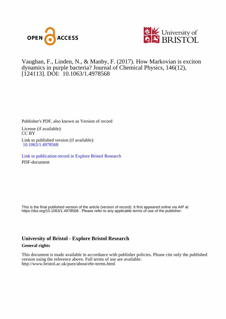
Figure 4 shows the trace distance used to calcu-late NBLP(ρ1, ρ2), where ρ1(0)= |1〉〈1| and ρ2(0)= |2〉〈2|.Increases in the trace distance are seen throughout the evo-lution up until it reaches its equilibrium state, showing thatnon-Markovian dynamics persist beyond the 200 fs indicatedin the Lindblad fitting result. However, it is clear that the most

FIG. 3. Histograms showing the degreeof non-Markovianity Q for different ini-tial states of a dimer coupled to a Brow-nian spectral density. The figure on theleft is for the case where the couplingbetween chromophores in the Hamilto-nian V is included as a fitting parame-ter. The right-hand figure is for a fixedHamiltonian.

124113-7 Vaughan, Linden, and Manby J. Chem. Phys. 146, 124113 (2017)

FIG. 4. The BLP measure of non-Markovianity D(ρ1(t), ρ2(t)) (Eq. (2))as a function of time for the HEOM calculation in Figure 2 where ρ1(0)= |1〉〈1 | and ρ2(0) = |2〉〈2 |. Regions of positive derivative correspond tonon-Markovian dynamics. The total non-Markovianity NBLP(ρ1, ρ2) = 0.14.

significant increases occur during the first 200 fs; thus, thetwo measures show a reasonably good agreement. The totalincrease in the trace distance over the 1 ps of dynamics givesa total non-Markovianity of NBLP(ρ1, ρ2) = 0.14, which is ofa similar size to other work quantifying non-Markovianity forthe Brownian spectral density.23

Overall, we find that for these parameters of the Brownianspectral density, the exciton dynamics shows small amountsof non-Markovianity in both the BLP measure and the Lind-blad fitting measure. The majority of the non-Markovianityoccurs in the first 200 fs of the dynamics, where we seethrough the Lindblad fitting measure that it results in reduced-amplitude oscillations in the site population, corresponding tothe reduced initial transfer of exciton density to the neighbour-ing chromophore. However, the Lindblad fit is still capable ofcapturing the key features of the dynamics, suggesting that forthese small values of the BLP metric, it may still be accept-able to adopt the Markov approximation provided the couplingstrength in the Hamiltonian is treated as a free parameter.

IV. DISCRETE SPECTRAL DENSITY

Here we investigate the effect that high-frequency, dis-crete modes of intra-molecular origin have on the degreeof non-Markovianity in the exciton dynamics. We look attwo key aspects. First, we investigate how the degree ofnon-Markovianity scales with the number of intra-molecularmodes. Second, we study the effect of modes resonant withthe gap in the excitonic spectrum by looking at the frequencydependence of the non-Markovianity for a single mode.

In order to get physically realistic parameters for thecoupling strength of intra-molecular modes, we performedquantum chemistry calculations on an isolated bacteriochloro-phyll-a molecule. The long phytyl chain was replaced with amethyl group to reduce computational expense; we anticipatethat this truncation will not affect our conclusions. Using Gaus-sian 0966 we used density functional theory (DFT) to optimisethe geometry and compute normal modes at the B3LYP/TZVPlevel of theory. To determine the coupling strength betweenthese vibrational modes and the electronic excitation, we usedtime dependent DFT (TDDFT) at the B3LYP/SVP level oftheory to compute the transition energy from the ground tofirst-excited state at discrete points along each normal mode

and fit this function to a straight line. The gradient ds of theresulting line gives the rate of change of excitation energywith displacement along the normal mode s, which the lin-ear approximation is related to the coupling parameters thatappear in Eq. (19) by

gs =

√~

2msωsds . (27)

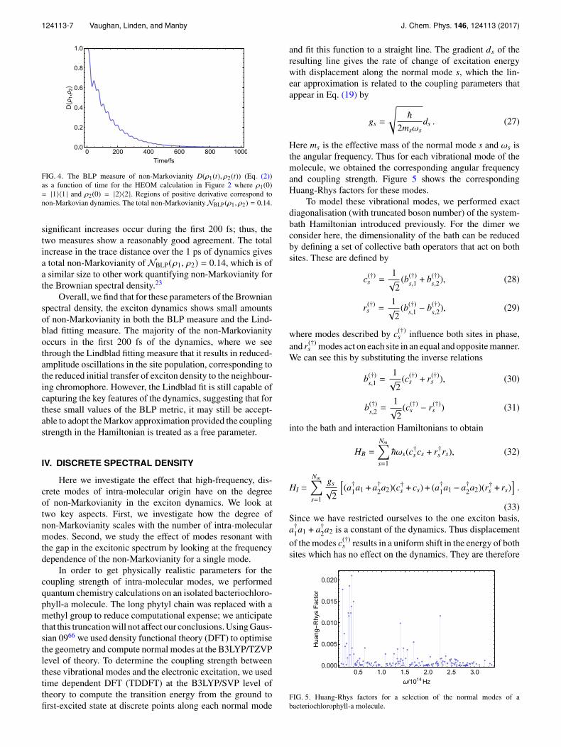
Here ms is the effective mass of the normal mode s and ωs isthe angular frequency. Thus for each vibrational mode of themolecule, we obtained the corresponding angular frequencyand coupling strength. Figure 5 shows the correspondingHuang-Rhys factors for these modes.

To model these vibrational modes, we performed exactdiagonalisation (with truncated boson number) of the system-bath Hamiltonian introduced previously. For the dimer weconsider here, the dimensionality of the bath can be reducedby defining a set of collective bath operators that act on bothsites. These are defined by

c(†)s =

1√

2(b(†)

s,1 + b(†)s,2), (28)

r(†)s =

1√

2(b(†)

s,1 − b(†)s,2), (29)

where modes described by c(†)s influence both sites in phase,

and r(†)s modes act on each site in an equal and opposite manner.

We can see this by substituting the inverse relations

b(†)s,1 =

1√

2(c(†)

s + r(†)s ), (30)

b(†)s,2 =

1√

2(c(†)

s − r(†)s ) (31)

into the bath and interaction Hamiltonians to obtain

HB =

Nm∑s=1

~ωs(c†s cs + r†s rs), (32)

HI =

Nm∑s=1

gs√

2

[(a†1a1 + a†2a2)(c†s + cs) + (a†1a1 − a†2a2)(r†s + rs)

].

(33)Since we have restricted ourselves to the one exciton basis,a†1a1 + a†2a2 is a constant of the dynamics. Thus displacement

of the modes c(†)s results in a uniform shift in the energy of both

sites which has no effect on the dynamics. They are therefore

FIG. 5. Huang-Rhys factors for a selection of the normal modes of abacteriochlorophyll-a molecule.

124113-8 Vaughan, Linden, and Manby J. Chem. Phys. 146, 124113 (2017)

FIG. 6. The typical degree of non-Markovianity as a function of the number of modes for initial states ρ1 = |1〉〈1 | and ρ2 = |2〉〈2 |. The modes are orderedfrom strongest to weakest coupling with Huang-Rhys factors ranging from 0.012 to 0.004 and are of frequency ω > 1014 Hz. Each calculation was run for atotal time of 1 ps. The measures NBLP and Q are defined in Eqs. (4) and (15), respectively.

ignored and we simply include in our simulations a single setof bath modes defined by r(†)

s ,

HB =

Nm∑s=1

~ωsr†s rs, (34)

HI =

2∑i=1

Nm∑s=1

(−1)i+1 gs√

2a†i ai(r

†s + rs). (35)

The advantage of this approach is that for a small number ofhigh-frequency modes ~ω � kbT , the boson number can betruncated (without significant loss of accuracy) at a level atwhich exact diagonalization can still be performed.

The modes we are modelling here represent delta peaks inthe spectral density. In the physical system, these delta peakswill be broadened due to interactions with the solvent environ-ment, which acts to dampen the non-equilibrium oscillations ofthe vibrational mode. The time scale for this damping processdepends upon the shape of the broadened peak. For Lorentzianbroadening, the peak is defined according to the function

C ′′(ω) =2√

2λγlω20ω

(ω2 − ω20)2 + 2γ2

l ω2

, (36)

where λ is the reorganisation energy, ω0 is the frequency ofthe vibrational mode, and γl the broadening factor such thatC ′′(ω) → δ(ω − ω0) as γl → 0. For this shape function non-equilibrium oscillations decay with e−γl t .27 Thus the resultsthat follow are accurate for modes where the time scale fordecay is long compared to the simulation time scale.

Here we look at how increasing the number of modesaffects the degree of non-Markovianity in the excitonic sub-system. To do this, we perform exact diagonalisation on thefull system-bath Hamiltonian and trace out the bath modes toobtain the excitonic reduced density matrix. For this calcula-tion, due to the computational expense of the exact diagonali-sation, we look only at the typical amount of non-Markovianityfor initial states where the exciton is fully localised, i.e., wecalculate NBLP(|1〉〈1| , |2〉〈2|) as well as the corresponding Qvalues for these initial states. Again the bath modes are takento be in a thermal initial state at temperature T = 288 K. Fig-ure 6 shows the amount of non-Markovianity present for asymmetric dimer coupled to Nm discrete modes from our DFTcalculations with frequencies ω > 1014 Hz. The modes wereordered by strength of coupling, with the strongest couplingmodes added first. The Huang-Rhys factors range from 0.012to 0.004. The Fock space of the bath is capped to have at mostNb = 15 quanta in total, which due to the small Huang-Rhys

FIG. 7. The degree of non-Markovian-ity as a function of the frequency of asingle mode coupled to symmetric (leftpanels) and asymmetric (right panels)chromophore dimers. In each case met-rics were extracted from 1 ps of dynam-ics. Each point in the upper plots rep-resents the non-Markovianity for a par-ticular pair of orthogonal initial states,whereas for the lower plots each pointis for a single initial state. Red andarrows indicate the frequency degener-ate with the gap between eigenvalues ofthe excitonic Hamiltonian.

124113-9 Vaughan, Linden, and Manby J. Chem. Phys. 146, 124113 (2017)

factors and high frequency of the modes is sufficient to captureessentially the exact dynamics. This was checked by increas-ing the boson number until convergence to a single result wasobserved. Each calculation is run for a total of 1 ps.

On the left of Figure 6, we can see that these discretemodes introduce a significant increase in the BLP trace dis-tance corresponding to non-Markovian dynamics. We see sim-ilar results on the right hand side for our Lindblad-fittingmetric. As the number of modes increases, the degree ofnon-Markovianity also increases. This is due to the increasedtotal coupling between the bath and the system as each newmode is included. The decreasing gradient is due to the order-ing of the modes that are added, starting from strongest toweakest coupling. These results suggest that the underdampedmodes that exhibit prolonged non-equilibrium oscillations inthe high-frequency region of the spectral density are likely tocontribute in a combined way to increase the non-Markovianity of the system dynamics. In other words, increas-ing the amount of structure in the higher frequency regimeof the spectral density will correspond with increased non-Markovianity.

A. Frequency dependence

Here we investigate how the frequency of a discretevibrational mode affects the degree of non-Markovianity.For completeness and since we are looking for resonanceswith the excitonic system, we study an asymmetric dimer(ε1 − ε2 = 200 cm−1 (3.77 × 1013 Hz)) as well as a sym-metric one (ε1 = ε2). In each case we couple the dimer to asingle mode with a Huang-Rhys factor, S = 0.1. We performa maximisation over 105 initial states chosen from a Lebe-dev grid65 over a hemi-sphere of the Bloch sphere, with theantipodes of these points forming their orthogonal counter-parts. The bath mode is taken to be a thermal state at T = 288 K.The BLP trace distance is then calculated between orthogonalpairs and the Markovianity measure NBLP(ρ1, ρ2) (Eq. (4))is calculated. We also apply our Lindblad fitting metric 〈Q〉,which is applied to the all trajectories resulting from the ini-tial states used for the BLP measure. The results are shown inFigure 7.

Figure 7 shows the results for both the symmetric andasymmetric dimers using the BLP measureNBLP and Lindbladfitting measure Q. For the BLP metric in both the symmet-ric and asymmetric cases, higher-frequency modes are foundto lead to more non-Markovian dynamics. The faster timescale of dynamics for the high-frequency modes results ina more rapid exchange of information between the systemand the environment and therefore a greater total exchangeover a picosecond of dynamics. Using this measure aloneone might conclude that there is nothing significant about thenon-Markovianity induced by resonant modes. However, forthe Lindblad fitting measure Q, we find a maximum in thedegree of non-Markovianity at the resonant frequencies. Thisimplies that although there is a greater total increase in the tracedistance for the case of higher frequency modes, the contribu-tion of that increase to deviations from the Lindblad model issmaller.

To understand why this is, we examined the time evolu-tion of the trace distance used to calculate the BLP measure.

Figure 8 shows three typical examples for a low-frequencymode (top panel), a resonant mode (middle panel), and a high-frequency mode (bottom panel). It can be seen that althoughthe total increase in the trace distance is greatest for the highfrequency modes, the amplitude of the trace distance oscil-lations is greatest for the near resonant modes. These largeamplitude oscillations in the BLP trace distance have a signifi-cant effect on the dynamics of the exciton, resulting in irregularoscillations in the site populations that the Lindblad equationsare unable to capture. The essential role resonant modes couldplay in assisting energy transport, which is to drive transi-tions between excitonic eigenstates and is observed for anessentially Markovian semi-classical treatment of the resonantmode.28 What we see here is that for a full quantum treat-ment, these resonant vibrational modes induce large-amplitudenon-Markovian oscillations that correspond to a maximal devi-ation from the Lindblad approximation. Whether this strongnon-Markovianity contributes to assisting energy transport isan open question.

FIG. 8. Examples of the time evolution of the trace distance for threetrajectories taken from the upper left graph in Figure 7. All trajectoriesare for the same pair of initial states of the exciton, ρ1 = |ψ〉〈ψ |, where|ψ〉 =

√0.79 |1〉 +

√0.21eiπ/4 |2〉 and ρ2 is the orthogonal state. Increas-

ing trace distance corresponds to non-Markovian dynamics. Upper: a modewell below resonance. Middle: a resonant mode. Lower: a mode well aboveresonance.

124113-10 Vaughan, Linden, and Manby J. Chem. Phys. 146, 124113 (2017)

We have also shown that when trying to determine theapplicability of Lindblad master equations using the BLPmetric, the most important feature is the amplitude of the trace-distance oscillations, rather than the total increase in the tracedistance. This is essentially an extension of the typical justifi-cations for a Markovian approximation but extended to applyto strict non-Markovianity measures. For small oscillationsin the BLP trace distance, it is easy for the monotonicallydecreasing trace distance of a Lindblad evolution to providea good fit. Similarly if the time scale for the oscillations issmall compared to the time scale of the phenomena of inter-est, then the dynamics can be well modelled by Lindbladdynamics.

V. STRUCTURED SPECTRAL DENSITY

Having looked at the non-Markovianity in the presenceof a broad spectral density to model a low-frequency phononbath, and a discrete spectral density to model intra-molecularmodes, we now turn our attention to a more realistic modelthat includes both. To do this, we include two environments:a discrete vibrational mode that is treated quantum mechan-ically on the same footing as the system Hamiltonian, and acontinuous bath as before.

The discrete bath mode is described as

HB1 = ~ωr†r, (37)

HI1 =

2∑i=1

(−1)i+1 g√

2a†i ai(r

† + r), (38)

where r(†) is the annihilation (creation) operator for the collec-tive vibrational mode defined in Section IV. The continuousbath mode, modelled by HB2 and HI 2 , is treated through theHEOM formalism; as before coupling strengths gs are definedby the Brownian spectral density (Eq. (22)).

To model the dynamics of the total Hamiltonian H = HS

+ HB1 + HI 1 + HB2 + HI 2 , we used HS + HB1 + HI 1 as the sys-tem Hamiltonian in the Phi software package. This effectivelycreates a system of n sites, where n is the dimension of theHilbert space of the Hamiltonian after truncation of the bosonnumber for mode r. Each site represents a state of the exci-tonic dimer and a state of the bath mode. We then ensured theHEOM bath coupled only to the excitonic system by correlat-ing coupling terms on sites with identical exciton states. Wethen traced out states associated with mode r to recover theexcitonic density matrix.

FIG. 10. The BLP trace distance as a function of time for the combinedHEOM and discrete mode calculation in Figure 9 where the initial stateswere ρ1(0) = |1〉〈1 | and ρ2(0) = |2〉〈2 |. The non-Markovianity measuresNBLP = 0.9.

Initially we chose the strongest coupling mode from ourDFT calculations whose frequency is ω > 1014 Hz. Figure 9shows the result for a mode frequency ω = 2.26 × 1014 Hz,Huang-Rhys factor S = 0.012, and for the |1〉 〈1| initial statewhich is a representative example. The optimal Lindblad wasfound by minimising 〈Q〉 over 105 pure initial states as inSections III and IV A. Here we see clearly the non-equilibriumoscillations that the undamped vibrational modes induce onthe system dynamics. In the HEOM calculations where onlythe phonon bath is included, the system reaches equilibriumat around 700 fs. Here we see that beyond this point non-equilibrium oscillations persist due to the undamped vibra-tional mode. This can also be seen in the BLP trace-distanceevolution in Figure 10, where oscillations continue throughoutthe evolution.

The BLP measure results in a non-Markovianity ofNBLP(ρ1, ρ2) = 0.9 which is around seven times larger thanfor the system coupled only to the phonon bath. The Lind-blad fitting on the other hand shows a smaller increase innon-Markovianity of approximately a factor of two, with Q= 0.013. An examination of Figure 9 illustrates the disparity,as although the total increase in the trace distance is greater,the effect on the dynamics has been minimal. This again illus-trates that the amplitude of increases in the trace distance isthe decisive factor in determining the applicability of Lindbladmaster equations.

In order to interpolate between the regime of a singlemode and the regime where many intra-molecular modes arecoupled to the system, we looked at the effect of a single effec-tive vibrational mode which combines the coupling strength

FIG. 9. An LH2 dimer coupled to a Brownian spectral density and a discrete vibrational mode with frequencyω = 2.26×1014 and Huang-Rhys factor S = 0.012at T = 288 K. Left: Site population for the full calculation (red) and the best fitting Lindblad evolution (blue). Right: trace distance between the fitted Lindbladevolution and the full calculation over time corresponding to non-Markovianity Q = 0.013.

124113-11 Vaughan, Linden, and Manby J. Chem. Phys. 146, 124113 (2017)

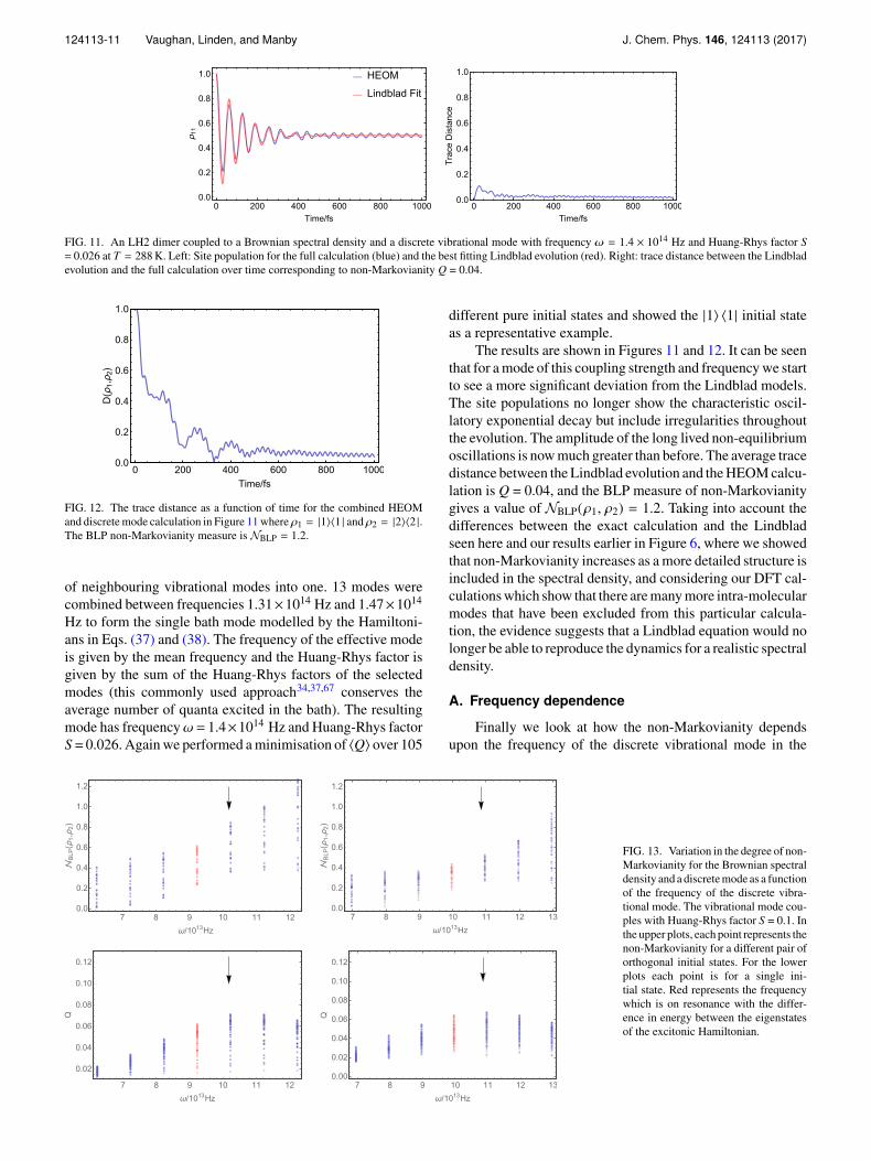
FIG. 11. An LH2 dimer coupled to a Brownian spectral density and a discrete vibrational mode with frequency ω = 1.4 × 1014 Hz and Huang-Rhys factor S= 0.026 at T = 288 K. Left: Site population for the full calculation (blue) and the best fitting Lindblad evolution (red). Right: trace distance between the Lindbladevolution and the full calculation over time corresponding to non-Markovianity Q = 0.04.

FIG. 12. The trace distance as a function of time for the combined HEOMand discrete mode calculation in Figure 11 where ρ1 = |1〉〈1 | and ρ2 = |2〉〈2 |.The BLP non-Markovianity measure is NBLP = 1.2.

of neighbouring vibrational modes into one. 13 modes werecombined between frequencies 1.31×1014 Hz and 1.47×1014

Hz to form the single bath mode modelled by the Hamiltoni-ans in Eqs. (37) and (38). The frequency of the effective modeis given by the mean frequency and the Huang-Rhys factor isgiven by the sum of the Huang-Rhys factors of the selectedmodes (this commonly used approach34,37,67 conserves theaverage number of quanta excited in the bath). The resultingmode has frequencyω = 1.4×1014 Hz and Huang-Rhys factorS = 0.026. Again we performed a minimisation of 〈Q〉 over 105

different pure initial states and showed the |1〉 〈1| initial stateas a representative example.

The results are shown in Figures 11 and 12. It can be seenthat for a mode of this coupling strength and frequency we startto see a more significant deviation from the Lindblad models.The site populations no longer show the characteristic oscil-latory exponential decay but include irregularities throughoutthe evolution. The amplitude of the long lived non-equilibriumoscillations is now much greater than before. The average tracedistance between the Lindblad evolution and the HEOM calcu-lation is Q = 0.04, and the BLP measure of non-Markovianitygives a value of NBLP(ρ1, ρ2) = 1.2. Taking into account thedifferences between the exact calculation and the Lindbladseen here and our results earlier in Figure 6, where we showedthat non-Markovianity increases as a more detailed structure isincluded in the spectral density, and considering our DFT cal-culations which show that there are many more intra-molecularmodes that have been excluded from this particular calcula-tion, the evidence suggests that a Lindblad equation would nolonger be able to reproduce the dynamics for a realistic spectraldensity.

A. Frequency dependence

Finally we look at how the non-Markovianity dependsupon the frequency of the discrete vibrational mode in the

FIG. 13. Variation in the degree of non-Markovianity for the Brownian spectraldensity and a discrete mode as a functionof the frequency of the discrete vibra-tional mode. The vibrational mode cou-ples with Huang-Rhys factor S = 0.1. Inthe upper plots, each point represents thenon-Markovianity for a different pair oforthogonal initial states. For the lowerplots each point is for a single ini-tial state. Red represents the frequencywhich is on resonance with the differ-ence in energy between the eigenstatesof the excitonic Hamiltonian.

124113-12 Vaughan, Linden, and Manby J. Chem. Phys. 146, 124113 (2017)

presence of a broad spectral density. The calculation per-formed is equivalent to that in Section IV A, but with theadditional presence of the Brownian spectral density. Figure 13shows the result for a symmetric and asymmetric dimer. Thedegree of non-Markovianity overall is significantly reduced,by approximately an order of magnitude, compared to thecalculations without the broad spectral density. The over-all trends however are similar. The BLP non-Markovianitymeasure again shows that high frequency modes induce thegreatest total trace-distance increase, due to the faster dynam-ics and therefore faster exchange of information. Again theLindblad fitting measure shows that there is a maximum in thenon-Markovianity. Interestingly, however, this maximum is nolonger at the frequency resonant with the system Hamiltonian(represented by the red points) but instead occurs at slightlyhigher frequencies. The shift seems to correspond to the shiftin the system coupling strength V required to fit a Lindblad tothe broad spectral density in Section III. If we take the reso-nant frequency of this fitted Hamiltonian (represented by thearrows), we find that it matches well with the new maximumin the non-Markovianity. This shows that the effective Hamil-tonian of the system is really changed by the interaction witha broad spectral density. It is possible that if light harvest-ing systems have evolved to take advantage of resonance withstrongly coupling discrete modes, they will have evolved suchthat the discrete mode is resonant with this effective systemHamiltonian.

VI. CONCLUSIONS

We have studied the excitonic dynamics of a chromophoredimer interacting with a vibrational environment in order toassess the applicability of Lindblad-type master equations formodelling photosynthetic energy transfer. The environmentwas modelled using both HEOM, to model a broad phononbath, and exact diagonalisation, to treat discrete vibrationalmodes of intra-molecular origin. To assess the validity ofLindblad master equations, we employed a recently developedmethod, based upon the trace distance, to measure the degreeof non-Markovianity by quantifying increases in the trace dis-tance between two evolutions. We also introduced and applieda measure of non-Markovianity which is based upon a generalparameterisation of a Lindblad master equation for the two-site case. This general parameterisation allows one to quantifythe distance between a general two-state quantum evolutionand the best-fitting Lindblad evolution.

For a Brownian spectral density, parameterised to fit thespectral density of the B777 complex, small amounts of non-Markovianity are observed using both metrics. In particular,the Lindblad fitting metric shows that this small amount of non-Markovianity results in slightly reduced-amplitude oscilla-tions in the site populations; however, overall the main featuresof the dynamics are well-captured by a Lindblad equation.

We found that to find the optimal Lindblad evolution,the system Hamiltonian had to be adjusted in such a waythat the coupling between the chromophores was increased.This is direct evidence that interaction with an environmentcan speed up the transfer process between chromophoresby introducing faster exciton transfer between the two sites.

However, whether similar adjustments to the Hamiltonianwould be required for a chromophore system of more thantwo sites is unknown. What this does show, however, is that itis not possible to accurately model exciton transfer by simplyemploying a Lindblad formulation with a system Hamiltonianparameterised separately.

We also investigated the significance of the frequencyof vibrational modes and whether any particular frequen-cies introduced greater non-Markovianity. We investigated thiswith and without the presence of a broad spectral density. Wefound that for the trace-distance metric of non-Markovianity,higher frequency modes introduce the most non-Markovianity.This is because higher frequency modes introduce faster oscil-lations in the trace distance resulting in a greater total increaseover a given time period.

For our Lindblad fitting measure of non-Markovianity,however, we found that, for the case excluding the broadspectral density, modes resonant with the difference betweeneigenvalues of the system Hamiltonian showed the greatestnon-Markovianity. The difference between the two measurescan be understood in terms of the amplitude of oscillationsin the trace distance. The modes resonant with the excitonicsystem induce the largest amplitude oscillations in the tracedistance. Thus the amplitude of oscillations in the trace dis-tance is the decisive feature by which to determine whetheror not the Lindblad approximation is a good fit, as opposed tosimply observing the total trace-distance increase. This resultapplies generally beyond applications to photosynthetic sys-tems. Whether the observed large amplitude oscillations in thetrace distance for resonant modes contributes to the recentlyobserved increase in energy transfer rates27–33 is left as anopen question.

For the case where the broad spectral density wasincluded, we found that the maximum non-Markovianityoccurred at slightly higher frequencies than the resonant fre-quency of the system Hamiltonian. We showed that this shiftis most likely due to the change in the effective Hamilto-nian of the system caused by the interaction with the broadspectral density. The Hamiltonian resulting from the Lindbladfit to the broad spectral density, which contained a param-eterised coupling strength V, was shown to have an eigen-state energy difference closer to the frequency of maximumnon-Markovianity.

Finally, we looked at whether a Lindblad master equa-tion would be capable of modelling the dynamics of a systemcoupled to a more realistic spectral density. In particular, westudied the effect of including some of the discrete vibra-tional modes that are responsible for the structure in the high-frequency region of the spectral density. For the dimer modelinteracting with only discrete vibrational modes, we found thatas the number of discrete vibrational modes was increased, thedegree of non-Markovianity also increased. For a model thatincluded a single discrete intra-molecular mode and a broadspectral density, the impact on the degree of non-Markovianitywas not very significant. However there are many such discreteintra-molecular modes, so in order to bridge the gap we mod-elled a single effective mode which incorporated the couplingstrengths of 13 modes of a similar frequency. Here we foundthat the evolution deviates from the Lindblad approximation,

124113-13 Vaughan, Linden, and Manby J. Chem. Phys. 146, 124113 (2017)

introducing irregular oscillations in the site populations. Con-sidering the number of discrete vibrational modes, and theirtendency to combine to increase non-Markovianity, we sus-pect that a Lindblad approximation may not be suitable formodelling such realistic spectral densities.

Note added in proof : A repository of all data generated inthe preparation of this paper is available online.68

ACKNOWLEDGMENTS

F.V. gratefully acknowledges funding from the EPSRCthrough the Bristol Centre for Complexity Sciences (GrantNo. EP/I013717/1).

1G. D. Scholes, G. R. Fleming, A. Olaya-Castro, and R. van Grondelle, Nat.Chem. 3, 763 (2011).

2N. Lambert, Y.-N. Chen, Y.-C. Cheng, C.-M. Li, G.-Y. Chen, and F. Nori,Nat. Phys. 9, 10 (2012).

3H. Lee, Y.-C. Cheng, and G. R. Fleming, Science 316, 1462 (2007).4G. S. Engel, T. R. Calhoun, E. L. Read, T.-K. Ahn, T. Mancal, Y.-C. Cheng,R. E. Blankenship, and G. R. Fleming, Nature 446, 782 (2007).

5G. Panitchayangkoon, D. Hayes, K. A. Fransted, J. R. Caram, E. Harel,J. Wen, R. E. Blankenship, and G. S. Engel, Proc. Natl. Acad. Sci. U. S. A.107, 12766 (2010).

6E. Collini, C. Y. Wong, K. E. Wilk, P. M. G. Curmi, P. Brumer, andG. D. Scholes, Nature 463, 644 (2010).

7E. Harel and G. S. Engel, Proc. Natl. Acad. Sci. U. S. A. 109, 706 (2012).8A. Ishizaki and G. R. Fleming, Annu. Rev. Condens. Matter Phys. 3, 333(2012).

9H. Bassereh, V. Salari, and F. Shahbazi, e-print arXiv:1504.04398v1 (2015).10F. Caruso, A. W. Chin, A. Datta, S. F. Huelga, and M. B. Plenio, J. Chem.

Phys. 131, 105106 (2009).11A. W. Chin, A. Datta, F. Caruso, S. F. Huelga, and M. B. Plenio, New J.

Phys. 12, 065002 (2010).12A. W. Chin, S. F. Huelga, and M. B. Plenio, Philos. Trans. R. Soc., A 370,

3638 (2012).13C. C. Forgy and D. A. Mazziotti, J. Chem. Phys. 141, 224111 (2014).14Y. Li, F. Caruso, E. Gauger, and S. C. Benjamin, New J. Phys. 17, 013057

(2015).15M. Mohseni, P. Rebentrost, S. Lloyd, and A. Aspuru-Guzik, J. Chem. Phys.

129, 174106 (2008).16M. B. Plenio and S. F. Huelga, New J. Phys. 10, 113019 (2008).17F. Caruso, A. W. Chin, A. Datta, S. F. Huelga, and M. B. Plenio, Phys. Rev.

A 81, 062346 (2010).18S. Hoyer, M. Sarovar, and K. B. Whaley, New J. Phys. 12, 065041 (2010).19A. Olaya-Castro, C. F. Lee, F. F. Olsen, and N. F. Johnson, Phys. Rev. B 78,

085115 (2008).20P. Rebentrost, M. Mohseni, and A. Aspuru-Guzik, J. Phys. Chem. B 113,

9942 (2009).21P. Rebentrost, M. Mohseni, I. Kassal, S. Lloyd, and A. Aspuru-Guzik, New

J. Phys. 11, 033003 (2009).22A. Ishizaki and G. R. Fleming, J. Chem. Phys. 130, 234110 (2009).23P. Rebentrost and A. Aspuru-Guzik, J. Chem. Phys. 134, 101103 (2011).24C. A. Mujica-Martinez, P. Nalbach, and M. Thorwart, Phys. Rev. E 88,

062719 (2013).25J. Liu, K. Sun, X. Wang, and Y. Zhao, Phys. Chem. Chem. Phys. 17, 8087

(2014).26F. Fassioli, A. Olaya-Castro, and G. D. Scholes, J. Phys. Chem. Lett. 3, 3136

(2012).27V. Butkus, L. Valkunas, and D. Abramavicius, J. Chem. Phys. 137, 044513

(2012).28A. W. Chin, J. Prior, R. Rosenbach, F. Caycedo-Soler, S. F. Huelga, and

M. B. Plenio, Nat. Phys. 9, 113 (2013).29A. Kolli, E. J. O’Reilly, G. D. Scholes, and A. Olaya-Castro, J. Chem. Phys.

137, 174109 (2012).

30P. Nalbach, C. A. Mujica-Martinez, and M. Thorwart, Phys. Rev. E 91,022706 (2013).

31F. Novelli, A. Nazir, G. H. Richards, A. Roozbeh, K. E. Wilk, P. M. G. Curmi,and J. A. Davis, J. Phys. Chem. Lett. 6, 4573 (2015).

32E. J. O’Reilly and A. Olaya-Castro, Nat. Commun. 5, 3012 (2014).33J. M. Womick and A. M. Moran, J. Phys. Chem. B 115, 1347 (2011).34J. Adolphs and T. Renger, Biophys. J. 91, 2778 (2006).35A. B. Doust, C. N. J. Marai, S. J. Harrop, K. E. Wilk, P. M. G. Curmi, and

G. D. Scholes, J. Mol. Biol. 344, 135 (2004).36A. Freiberg, M. Ratsep, K. Timpmann, and G. Trinkunas, Chem. Phys. 357,

102 (2009).37M. Ratsep and A. Freiberg, J. Lumin. 127, 251 (2007).38A. Rivas, S. F. Huelga, and M. B. Plenio, Rep. Prog. Phys. 77, 094001

(2014).39M. M. Wolf and J. I. Cirac, Commun. Math. Phys. 279, 147 (2008).40A. Rivas, S. F. Huelga, and M. B. Plenio, Phys. Rev. Lett. 105, 050403

(2010).41S. C. Hou, S. L. Liang, and X. X. Yi, Phys. Rev. A 91, 012109 (2015).42D. Chruscinski and S. Maniscalco, Phys. Rev. Lett. 112, 120404 (2013).43B. Bylicka, D. Chruscinski, and S. Maniscalco, e-print arXiv:1301.2585v1

(2013).44R. Vasile, S. Maniscalco, M. G. A. Paris, H.-P. Breuer, and J. Piilo, Phys.

Rev. A 84, 052118 (2011).45X. M. Lu, X. Wang, and C. P. Sun, Phys. Rev. A 82, 042103 (2010).46E.-M. Laine, J. Piilo, and H.-P. Breuer, Phys. Rev. A 81, 062115 (2010).47H.-P. Breuer, E.-M. Laine, and J. Piilo, Phys. Rev. Lett. 103, 210401 (2009).48S. Luo, S. Fu, and H. Song, Phys. Rev. A 86, 044101 (2012).49D. Girolami and G. Adesso, Phys. Rev. Lett. 108, 150403 (2012).50D. Chruscinski, A. Kossakowski, and A. Rivas, Phys. Rev. A 83, 052128

(2011).51M. J. W. Hall, J. D. Cresser, L. Li, and E. Andersson, Phys. Rev. A 89,

042120 (2014).52S. Lorenzo, F. Plastina, and M. Paternostro, Phys. Rev. A 88, 020102

(2013).53S. Wimann, A. Karlsson, E.-M. Laine, J. Piilo, and H.-P. Breuer, Phys. Rev.

A 86, 062108 (2012).54J. Liu, X. M. Lu, and X. Wang, Phys. Rev. A 87, 042103 (2013).55K. Lendi, J. Phys. A: Math. Gen. 20, 15 (1999).56V. Gorini, A. Kossakowski, and E. C. G. Sudarshan, J. Math. Phys. 17, 821

(1976).57M. Znidaric, Phys. Rev. A 91, 052107 (2015).58F. Fassioli, A. Olaya-Castro, S. Scheuring, J. N. Sturgis, and N. F. Johnson,

Biophys. J. 97, 2464 (2009).59A. Kell, X. Feng, M. Reppert, and R. Jankowiak, J. Phys. Chem. B 117,

7317 (2013).60Y. Tanimura and R. Kubo, J. Phys. Soc. Jpn. 58, 1199 (1989).61H. Liu, L. Zhu, S. Bai, and Q. Shi, J. Chem. Phys. 140, 134106 (2014).62T. Renger and R. A. Marcus, J. Chem. Phys. 116, 9997 (2002).63R. J. Cogdell, A. Gall, and J. Kohler, Q. Rev. Biophys. 39, 227 (2006).64J. Strumpfer and K. Schulten, J. Chem. Theory Comput. 8, 2808 (2012).65V. I. Lebedev, Comput. Math. Math. Phys. 16, 10 (1976).66M. J. Frisch, G. W. Trucks, H. B. Schlegel, G. E. Scuseria, M. A. Robb,

J. R. Cheeseman, G. Scalmani, V. Barone, G. A. Petersson, H. Nakatsuji,X. Li, M. Caricato, A. V. Marenich, J. Bloino, B. G. Janesko, R. Gomperts,B. Mennucci, H. P. Hratchian, J. V. Ortiz, A. F. Izmaylov, J. L.Sonnenberg, D. Williams-Young, F. Ding, F. Lipparini, F. Egidi, J. Goings,B. Peng, A. Petrone, T. Henderson, D. Ranasinghe, V. G. Zakrzewski, J. Gao,N. Rega, G. Zheng, W. Liang, M. Hada, M. Ehara, K. Toyota, R. Fukuda,J. Hasegawa, M. Ishida, T. Nakajima, Y. Honda, O. Kitao, H. Nakai,T. Vreven, K. Throssell, J. A. Montgomery, Jr., J. E. Peralta, F. Ogliaro,M. J. Bearpark, J. J. Heyd, E. N. Brothers, K. N. Kudin, V. N. Staroverov,T. A. Keith, R. Kobayashi, J. Normand, K. Raghavachari, A. P. Rendell,J. C. Burant, S. S. Iyengar, J. Tomasi, M. Cossi, J. M. Millam, M. Klene,C. Adamo, R. Cammi, J. W. Ochterski, R. L. Martin, K. Morokuma,O. Farkas, J. B. Foresman, and D. J. Fox, gaussian 09 Revision A.03,Gaussian, Inc., Wallingford, CT, 2009.

67L. Gisslen and R. Scholz, Phys. Rev. B 80, 115309 (2009).68F. Vaughan, N. Linden, and F. R. Manby, Open-access repository, https://

doi.org/10.5523/bris.16l9cl5elvnr02x2aunzxhqsmp (2017).