vascat - dept.aoe.vt.educdhall/courses/micromaps/vascat_final.pdf · appendix c: matlab earth...
TRANSCRIPT

VASCAT
(Virginia Satellite for Carbon-monoxide Analysis and Tabulation)
MicroMAPS Host Satellite Design Proposal
Michael P. Belcher Ann W. Bergquist Joseph G. Bidwell Kevin D. Earle Scott E. Lennox Daniel Pedraza
Christine R. Rogers Matthew C. VanDyke Richard G. Winski
August 27, 2002
Christopher D. Hall Aerospace and Ocean Engineering Department
Virginia Polytechnic Institute and State University 215 Randolph Hall
Blacksburg, VA 24061
[email protected] (540) 231-2314 fax (540) 231-9632
ii
Table of Contents List of Figures ............................................................................................................................................... iii List of Tables..................................................................................................................................................iv List of Tables..................................................................................................................................................iv List of Abbreviations.......................................................................................................................................v List of Symbols ..............................................................................................................................................vi Chapter 1: Introduction and Problem Definition.............................................................................................8 1.1 Descriptive scenario ..................................................................................................................................8 1.2 Scope.........................................................................................................................................................9 1.3 Needs, alterables, and constraints..............................................................................................................9 1.4 Value system design................................................................................................................................10 1.5 Summary and conclusions.......................................................................................................................12 Chapter 2: Satellite Configuration and Components .....................................................................................13 2.1 Configuration ..........................................................................................................................................13 2.2 Structure ..................................................................................................................................................15 2.2.1 Requirements........................................................................................................................................15 2.2.2 Launch vehicle selection ......................................................................................................................16 2.2.3 Bus structure.........................................................................................................................................16 2.2.4 Structure configuration.........................................................................................................................19 2.2.5 Component layout ................................................................................................................................20 2.3 ADCS ......................................................................................................................................................21 2.3.1 Attitude control architecture.................................................................................................................21 2.3.2 Attitude control modes .........................................................................................................................22 2.3.3 Disturbance torques..............................................................................................................................23 2.3.4 Hardware ..............................................................................................................................................25 2.4 Power ......................................................................................................................................................31 2.4.1 Power Requirements ............................................................................................................................32 2.4.2 Power Generation.................................................................................................................................33 2.4.3 Energy Storage .....................................................................................................................................35 2.5 Thermal ...................................................................................................................................................36 2.6 Communication .......................................................................................................................................42 2.6.1 Uplink...................................................................................................................................................42 2.6.2 Downlink..............................................................................................................................................43 2.6.3 AMSAT................................................................................................................................................44 2.7 Command and data handling...................................................................................................................44 2.8 Summary .................................................................................................................................................44 Chapter 3: Mission Operations......................................................................................................................45 3.1 Orbits.......................................................................................................................................................45 3.1.1 Coverage ..............................................................................................................................................45 3.1.2 Orbit prediction ....................................................................................................................................46 3.1.3 Orbit simulation....................................................................................................................................46 3.1.4 Orbit characteristics..............................................................................................................................46 3.1.5 Lifetime ................................................................................................................................................47 3.2 Summary .................................................................................................................................................50 Chapter 4: Cost Analysis...............................................................................................................................51 Chapter 5: Summary, Conclusions, and Remaining Work............................................................................53 References .....................................................................................................................................................54 Appendix A: MATLAB Power Code...........................................................................................................56 Appendix B: HokieSat Loop Antenna...........................................................................................................58 Appendix C: MATLAB Earth Ground Coverage Code ...............................................................................59 Appendix D: MATLAB Disturbance Torque and Attitude Actuator Sizing Code.......................................62

iii
List of Figures
Figure 1: Objective hierarchy chart...............................................................................................................11 Figure 2: Internal configuration of HokieSat7 ...............................................................................................13 Figure 3: External configuration of HokieSat7 ..............................................................................................14 Figure 4: VASCAT external configuration ...................................................................................................15 Figure 5: Illustration of isogrid construction15 ..............................................................................................20 Figure 6: Ithaco CES sensor head diagram11.................................................................................................26 Figure 7: An isometric diagram of the BEI Systron Donner QRS-11 rate gyro17 .........................................27 Figure 8: A three view drawing of the Ithaco IM-103 magnetometer11 ........................................................28 Figure 9: A cut-away diagram showing the interior of an Ithaco Type A momentum wheel11.....................29 Figure 10: External configuration diagram of an Ithaco TR30CFR magnetic torque bar11...........................31 Figure 11: VASCAT power model ...............................................................................................................34 Figure 12: Cycle life versus DOD20 ..............................................................................................................35 Figure 13: Uplink transceiver5 ......................................................................................................................42 Figure 14: Downlink transmitter5..................................................................................................................43 Figure 15: Lifetime plotted as a function of altitude .....................................................................................47 Figure 16: Lifetime plotted as a function of drag coefficient for a 400 km altitude orbit .............................48 Figure 17: Lifetime plotted as a function of drag coefficient for a 500 km altitude orbit .............................48 Figure 18: Lifetime plotted as a function of drag area for a 400 km altitude orbit .......................................49 Figure 19: Lifetime plotted as a function of drag area for a 500 km altitude orbit .......................................49 Figure 20: Lifetime plotted as a function of orbit inclination .......................................................................50 Figure 21: Loop antenna assembly from HokieSat drawing package ...........................................................58 Figure 22: Copper tube loop from HokieSat drawing package .....................................................................58

iv
List of Tables
Table 1: List of needs, alterables, and constraints for host satellite design .....................................................9 Table 2: List of objectives and their associated subsystem ...........................................................................10 Table 3: Mass budget by subsystem..............................................................................................................15 Table 4: Structural requirements16.................................................................................................................16 Table 5: Limiting loads on structure during launch ......................................................................................17 Table 6: Trade study of component mounting techniques.............................................................................21 Table 7: MicroMAPS imposed attitude requirements19 ................................................................................22 Table 8: Estimated structural properties of the VASCAT.............................................................................24 Table 9: Estimated orbital properties of the VASCAT .................................................................................24 Table 10: Estimated disturbance torques.......................................................................................................25 Table 11: Properties of the Ithaco CES11 ......................................................................................................26 Table 12: Properties of the Valley Forge Composite Technologies Sun Sensor18 ........................................27 Table 13: Properties of the BEI Systron Donner QRS-11 rate gyro17 ...........................................................27 Table 14: Properties of the Ithaco IM-103 magnetometer11 ..........................................................................28 Table 15: VASCAT orbital and environmental properties............................................................................29 Table 16: Properties of the Ithaco TW-4A12 momentum wheel11 ................................................................30 Table 17: Properties of the Ithaco TR30CFR magnetic torque bar11.............................................................31 Table 18: Component power requirements ...................................................................................................32 Table 19: Daylight and eclipse power budget ...............................................................................................33 Table 20: Design parameters for preliminary VASCAT thermal analysis ....................................................37 Table 21: VASCAT Temperature Limits (°C) ..............................................................................................37 Table 22: Component internal power dissipations ........................................................................................39 Table 23: Environmental fluxes in space (W/m2) .........................................................................................39 Table 24: Surface properties..........................................................................................................................39 Table 25: Temperatures of the VASCAT components .................................................................................41 Table 26: Uplink receiver specifications5......................................................................................................43 Table 27: Downlink transmitter specifications5 ............................................................................................43 Table 28: The VASCAT cost estimate using PECM20..................................................................................52

v
List of Abbreviations
ADCS Attitude determination and control system
AMSAT Amateur Satellite
CER Cost estimation relationships
CES Conical Earth sensor
DOD Depth of discharge
ECA Earth center angle
GASCAN Getaway special canister
GSFC Goddard Space Flight Center
ICD Interface control document
IR Infrared
LaRC Langley Research Center
LEO Low-Earth orbit
MAPS Measurement of Air Pollution from Satellites
µMAPS MicroMAPS Gas Filter Correlation Radiometer
MTB Magnetic torque bar
MOE Measure of effectiveness
NASA National Aeronautics and Space Administration
NiCd Nickel cadmium
NiMH Nickel metal-hydride
PECM Parametric cost estimation method
RTG Radio-isotope thermoelectric generator
SHELS Shuttle Hitchhiker Experiment Launch System
SINDA Systems Integrated Numerical Differential Analyzer
STK Satellite Tool Kit
TCS Thermal control system
UHF Ultra-high frequency
VASCAT Virginia Satellite for Carbon-monoxide Analysis and Tabulation

vi
List of Symbols
ℑ View factor
A Area
a Semi-major axis
B Magnetic field strength
b Plate width
Cd Drag coefficient
cg Location of the center of gravity
Cp Specific heat capacity
c Speed of light
cpa Location of the center of atmospheric pressure
cps Location of the center of solar pressure
D Magnetic dipole strength
E Modulus of elasticity
Fcr Critical load
fnat Natural frequency
Fs Solar constant
G Conduction coupling value
g Gravitational constant
h Angular momentum
i Inclination
Ix, Iy, Iz Moments of inertia
k Thermal conductivity
k’ Boundary condition factor
l Length
M Bending moment
m Mass
mc Cell mass
Nc Number of cells
P Power
Paxial Axial limit load
Peq Equivalent axial load
Pult Ultimate load
Q Net heat flux

vii
q Reflectance factor
R Moment arm, orbital radius
T Temperature
Ta Atmospheric pressure torque
Td Total disturbance torque
Tg Gravity gradient torque
Tm Magnetic torque
Tsp Solar pressure torque
t Thickness
α Absorptivity
∆t Change in time
δ Beam deflection
ε Emissivity
µ Gravitational constant
ν Poisson’s ratio
ρ Atmospheric density
σ Axial stress, Steffan-Boltzmann constant
θ Off-nadir angle
θa Allowable angular error
8
Chapter 1: Introduction and Problem Definition
1.1 Descriptive scenario
Scientists at the National Aeronautics and Space Administration’s (NASA) Langley Research
Center (LaRC) developed an instrument to study pollution in the Earth’s atmosphere from space. This
Earth-observing instrument, known as the MicroMAPS Gas Filter Correlation Radiometer (µMAPS), a
smaller version of the original Measurement of Air Pollution from Satellites (MAPS) instrument, measures
carbon monoxide levels in the troposphere. Researchers study the characteristics and movement of air
pollution from data acquired. Following cancellation of the Clarke mission, upon which the µMAPS
instrument was scheduled to ride, scientists at LaRC began to formulate new ideas for getting the
instrument into space. One alternative mission requests that a single satellite be designed whose sole
purpose is to house and support the µMAPS instrument. Virginia Tech is chosen to design this satellite,
based on its existing nanosatellite design, HokieSat. This report describes the host satellite design for the
µMAPS instrument.
The new host satellite will be designed, built and tested in Virginia through collaboration of
Virginia Tech, the University of Virginia, Old Dominion University, the Virginia Space Grant Consortium,
and LaRC. Virginia Tech is responsible for the design of the host satellite, including the structure and all
internal subsystems. The host satellite design is based on Virginia Tech’s HokieSat, part of a project
supported by NASA’s Goddard Space Flight Center (GSFC). The host satellite is designed to house and
support the µMAPS instrument, and possibly a camera, with a three-year lifetime.
The host satellite will be placed into a 400 km circular orbit with an inclination of 51.6o. The host
satellite can launch on a shuttle hitchhiker system such as the Shuttle Hitchhiker Experiment Launch
System (SHELS) or the getaway special canister (GASCAN), or as a secondary payload on an expendable
launch vehicle. To relay data from the instrument to the ground, the host satellite uses Amateur Satellite
(AMSAT) groundstations around the world to downlink data continuously.
9
1.2 Scope
The focus of this proposal is the design of a satellite that is capable of supporting the µMAPS
instrument and mission. The structure of this satellite, as well as all internal and external subsystem
components are designed and sized. The satellite must carry the necessary power generation and energy
storage systems. The ADCS is designed to fulfill µMAPS orientation requirements. The method of ground
communication is chosen for adequate transmission of necessary data.
The design process begins with an established nanosatellite design. This design is modified in all
respects to fulfill our scope. The µMAPS host satellite design must be complete by the end of the current
semester. HokieSat provides a first iteration on the desired satellite, therefore allowing for a complete
design in the time allotted. Launch vehicle suggestions are included in the scope of the project; however,
this design does not limit launch vehicle selection.
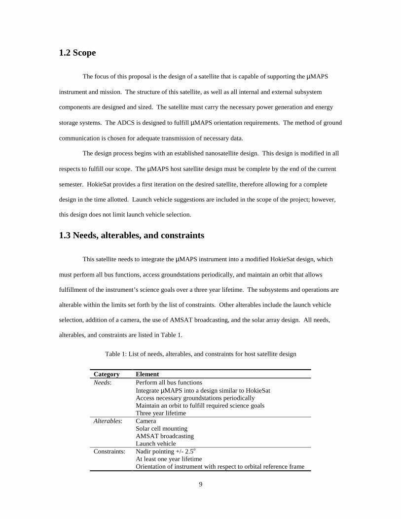
1.3 Needs, alterables, and constraints
This satellite needs to integrate the µMAPS instrument into a modified HokieSat design, which
must perform all bus functions, access groundstations periodically, and maintain an orbit that allows
fulfillment of the instrument’s science goals over a three year lifetime. The subsystems and operations are
alterable within the limits set forth by the list of constraints. Other alterables include the launch vehicle
selection, addition of a camera, the use of AMSAT broadcasting, and the solar array design. All needs,
alterables, and constraints are listed in Table 1.
Table 1: List of needs, alterables, and constraints for host satellite design
Category Element Needs: Perform all bus functions Integrate µMAPS into a design similar to HokieSat Access necessary groundstations periodically Maintain an orbit to fulfill required science goals Three year lifetime Alterables: Camera Solar cell mounting AMSAT broadcasting Launch vehicle Constraints: Nadir pointing +/- 2.5o At least one year lifetime Orientation of instrument with respect to orbital reference frame
10
1.4 Value system design
The value system design (VSD) is used to evaluate iterations on the HokieSat design. The VSD
puts all mission objectives into a hierarchy beginning with the top-level objective: optimize the satellite
design. Maximizing the performance objectives and minimizing the cost objectives optimizes the satellite
design. The performance and cost objectives are described in this section.
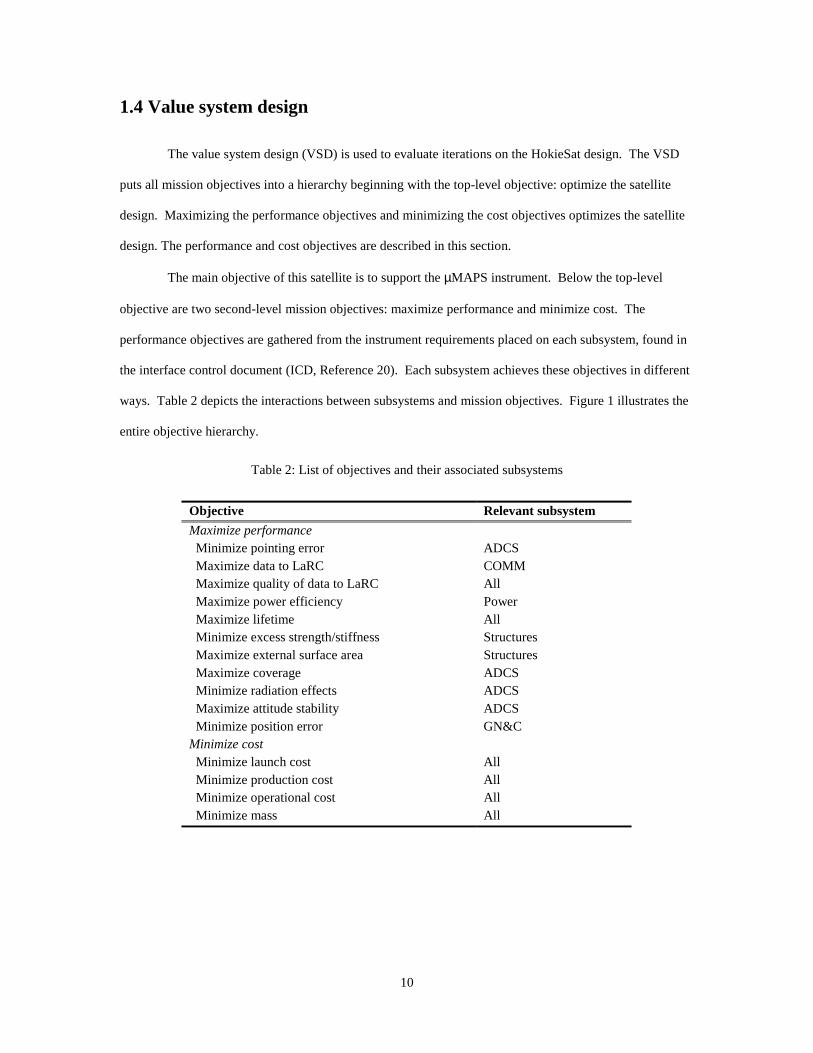
The main objective of this satellite is to support the µMAPS instrument. Below the top-level
objective are two second-level mission objectives: maximize performance and minimize cost. The
performance objectives are gathered from the instrument requirements placed on each subsystem, found in
the interface control document (ICD, Reference 20). Each subsystem achieves these objectives in different
ways. Table 2 depicts the interactions between subsystems and mission objectives. Figure 1 illustrates the
entire objective hierarchy.
Table 2: List of objectives and their associated subsystems
Objective Relevant subsystem
Maximize performance Minimize pointing error ADCS Maximize data to LaRC COMM Maximize quality of data to LaRC All Maximize power efficiency Power Maximize lifetime All Minimize excess strength/stiffness Structures Maximize external surface area Structures Maximize coverage ADCS Minimize radiation effects ADCS Maximize attitude stability ADCS Minimize position error GN&C Minimize cost Minimize launch cost All Minimize production cost All Minimize operational cost All Minimize mass All

11
Figure 1: Objective hierarchy chart
This objective hierarchy is further divided into sub-levels of performance and cost that are
associated with measures of effectiveness (MOEs). For example, a MOE for the ADCS is pointing error of
the satellite. This MOE is minimized to achieve greater precision in attitude maneuvers. The
communications subsystem maximizes data quality transferred to ground stations as one of its performance
objectives. An objective of the structural engineers is to maximize the available surface area to allow for
body mounted solar cells.
Several performance MOEs are comprised of separate quantities. The performance of the satellite
structure accounts for material strength and stiffness. These quantities depend on material characteristics.
Maximizing the efficiency of the power system depends on all internal components of the satellite such as
the computer, ADCS components, and the µMAPS instrument. The communications system performance
also depends upon factors, which affect the entire satellite, such as the radiation dose.
12
1.5 Summary and conclusions
Chapter 1 introduces the need for a satellite to house the µMAPS instrument. The problem
definition identifies the scope, boundaries, and relevant elements of the problem. Students at Virginia Tech
modify an existing nanosatellite design, HokieSat, to fit the needs of the µMAPS instrument. The
following chapters outline the components pre-existing to HokieSat, and the detailed modifications made to
each subsystem to arrive at a host satellite design.

13
Chapter 2: Satellite Configuration and Components
Chapter 2 presents the VASCAT configuration and subsystem components. The configuration
and the subsystem components are based on the HokieSat design. This chapter defines the subsystem
designs and presents the analyses leading up to these designs. The satellite subsystems include the
structure, the attitude determination and control system, the power system, the thermal system and the
communications system.
2.1 Configuration
The configuration of this satellite is based on an existing satellite design. HokieSat is a hexagonal
nanosatellite with a major diameter of 18 inches and a height of 13.725 inches. It draws power from body-
mounted solar cells covering approximately 80% of each side. HokieSat uses an electric propulsion system
whose thrusters protrude from four sides of the structure. The HokieSat bus is made of a 6061-T6
aluminum alloy cut into an isogrid pattern. All eight sides are 0.23” thick isogrid. The six side panels are
composite isogrid-skin. The 0.02” skin is bonded to the isogrid to form a 0.25” total thickness. All internal
components are mounted to the interior of the six side panels and the two end panels. The external
communications components are mounted to the exterior of the two end panels. Figure 2 and Figure 3
illustrate this configuration.8
Figure 2: Internal configuration of HokieSat7
14
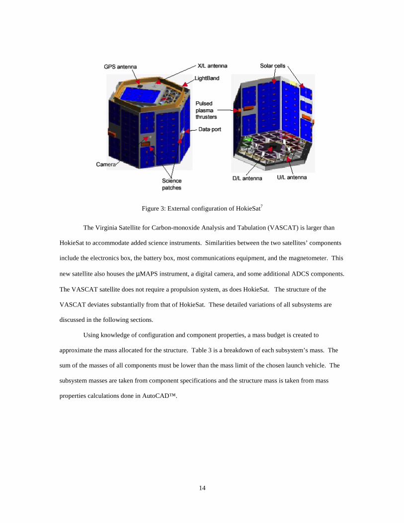
Figure 3: External configuration of HokieSat7
The Virginia Satellite for Carbon-monoxide Analysis and Tabulation (VASCAT) is larger than
HokieSat to accommodate added science instruments. Similarities between the two satellites’ components
include the electronics box, the battery box, most communications equipment, and the magnetometer. This
new satellite also houses the µMAPS instrument, a digital camera, and some additional ADCS components.
The VASCAT satellite does not require a propulsion system, as does HokieSat. The structure of the
VASCAT deviates substantially from that of HokieSat. These detailed variations of all subsystems are
discussed in the following sections.
Using knowledge of configuration and component properties, a mass budget is created to
approximate the mass allocated for the structure. Table 3 is a breakdown of each subsystem’s mass. The
sum of the masses of all components must be lower than the mass limit of the chosen launch vehicle. The
subsystem masses are taken from component specifications and the structure mass is taken from mass
properties calculations done in AutoCAD™.

15
Table 3: Mass budget by subsystem
Subsystem Total mass, kg Science 6.4 ADCS 14.0 C&DH 2.8 Power 1.7 Communications 0.4 Structure 11.4 TOTAL 36.7
2.2 Structure
The structure of VASCAT is designed with adequate surface area for body mounted solar cells
and adequate volume to house all components including the µMAPS instrument. The structure of the
VASCAT is 0.67 m in major diameter and 1 m high. Figure 4 is an illustration of the VASCAT. The
satellite’s dimensions are small enough to allow for 0.85 m on each side in the payload fairing.
Figure 4: VASCAT external configuration
2.2.1 Requirements
Design and analysis of primary structural components necessitates the derivation of structural
requirements. Table 4 lists all requirements relevant to this preliminary design. Mass and size of the

16
structure are limited by the launch vehicle selected, and the size and mass of the primary payload, should
this satellite be a hitchhiker. The launch vehicle selected also sets requirements on the strength of the
structure. The orbit altitude desired, and therefore the launch vehicle, restricts the mass of the structure.
All primary and secondary structural components should meet the pre-determined mass allocation (see
Table 3).16
Table 4: Structural requirements16
Requirement Description Required information General shape and purpose
Provides load paths between supported components and launch vehicle; fits inside
payload fairing
Configuration, spacecraft component level layout
Strength Survives loads induced during launch; withstands on-orbit loads, cyclic over
lifetime
Load factors from launch vehicle; mass properties of spacecraft
Stiffness Meets launch vehicle fundamental frequency requirement
Dynamic envelope of launch vehicle environment; mass
properties of spacecraft Mechanical
interface Meets launch vehicle flatness requirements;
adaptable to launch vehicle attachment interface
Interface requirements inside payload fairing
Mass Meets target mass allotment; meets launch vehicle mass limitation
Allocated mass
2.2.2 Launch vehicle selection
Since the launch of this satellite is uncertain, no launch vehicle is desired more than another. The
VASCAT can either launch on the Space Shuttle as a hitchhiker payload, or as a secondary payload on any
other launch vehicle. The structure is designed based on a worst case launch environment scenario. The
Athena I launch vehicle is therefore chosen for structural analysis due to its relatively high launch loads.
The Athena I is produced by Lockheed Martin. It has a payload fairing diameter of 2.36 m and a height of
8.81 m, and is capable of carrying up to 794 kg to LEO.10
2.2.3 Bus structure
Configuration and component layout guides the sizing of all primary structures. However, these
dimensions change with strength requirements placed on the satellite. The challenge is to design a system
to house all components, survive the launch environment, and withstand cyclic on-orbit loads.15 This
section describes the process used to define dimensions of the VASCAT’s primary structure.
17
The International Reference Guide to Space Launch Systems states that the Athena I
environment’s limit load factors are 8.1-g’s axially and 1.8-g’s laterally. A factor of safety of 2 is used
during static calculations to ensure that the structure withstands these loads during launch. 20 The
fundamental frequency of the VASCAT must be above 15 Hz laterally and 30 Hz longitudinally. The type
of structure is chosen during dynamic calculations to ensure that the natural frequency of the satellite meets
this stiffness requirement.
The mechanical interface is chosen for integration with the launch vehicle such that it meets the
payload fairing’s flatness requirement and coincides with its bolt hole patterns and other attachment
restrictions. 20 The VASCAT mass budget (Table 3) allows for the structure to be approximately 30% of
the total mass of the satellite.
2.2.3.1 Ultimate loads
An ultimate load for the bus structure is calculated for tensile strength sizing.
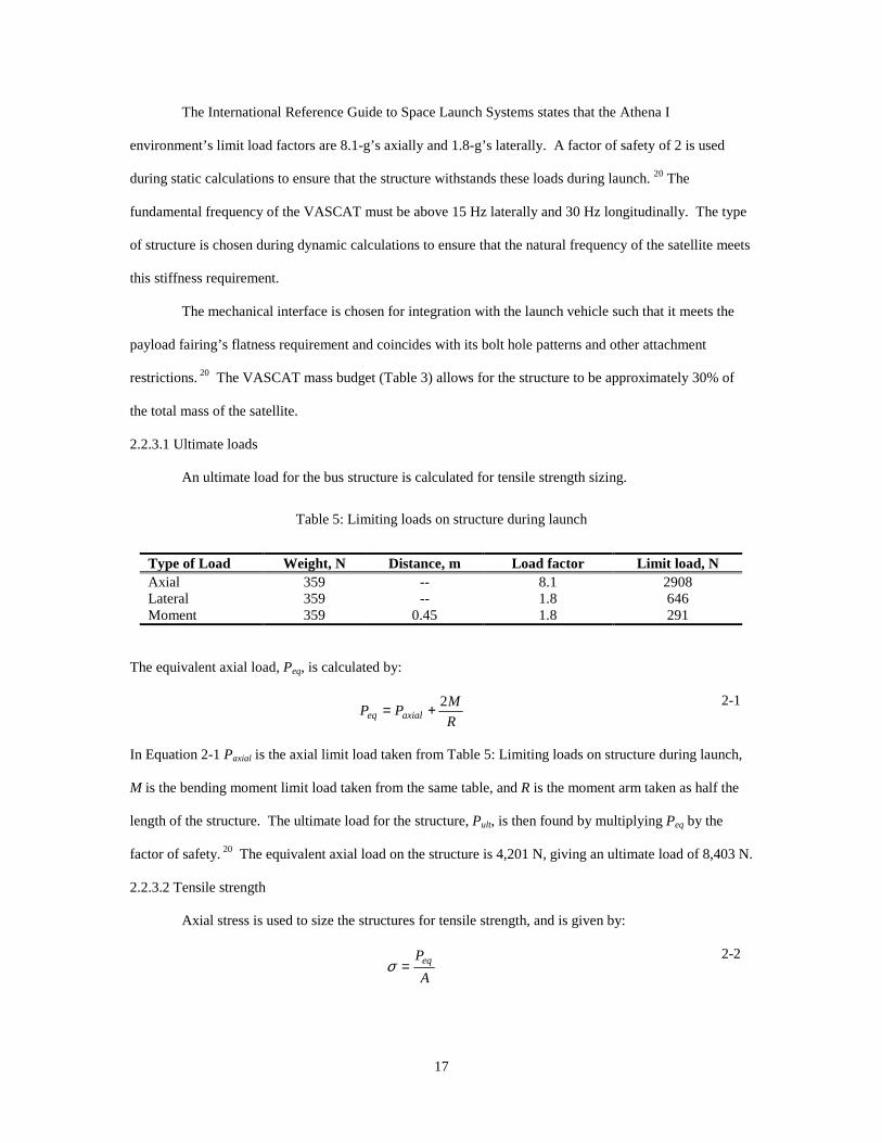
Table 5: Limiting loads on structure during launch
Type of Load Weight, N Distance, m Load factor Limit load, N Axial 359 -- 8.1 2908 Lateral 359 -- 1.8 646 Moment 359 0.45 1.8 291
The equivalent axial load, Peq, is calculated by:
R
MPP axialeq
2+= 2-1
In Equation 2-1 Paxial is the axial limit load taken from Table 5: Limiting loads on structure during launch,
M is the bending moment limit load taken from the same table, and R is the moment arm taken as half the
length of the structure. The ultimate load for the structure, Pult, is then found by multiplying Peq by the
factor of safety. 20 The equivalent axial load on the structure is 4,201 N, giving an ultimate load of 8,403 N.
2.2.3.2 Tensile strength
Axial stress is used to size the structures for tensile strength, and is given by:
A
Peq=σ 2-2
18
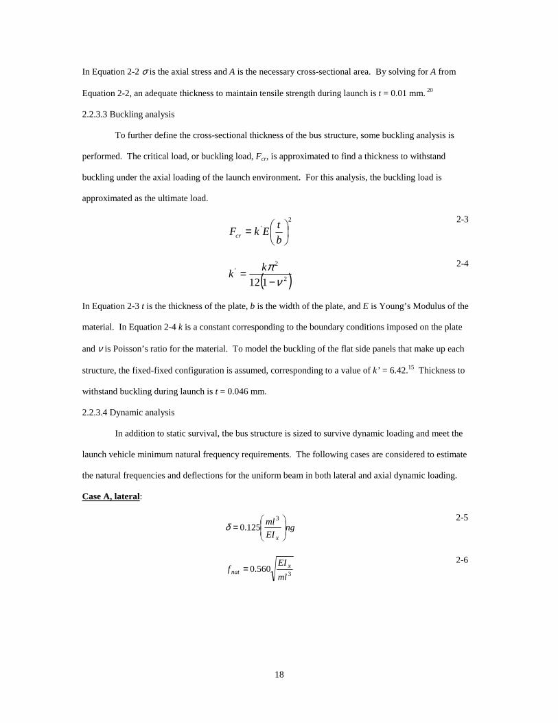
In Equation 2-2 σ is the axial stress and A is the necessary cross-sectional area. By solving for A from
Equation 2-2, an adequate thickness to maintain tensile strength during launch is t = 0.01 mm. 20
2.2.3.3 Buckling analysis
To further define the cross-sectional thickness of the bus structure, some buckling analysis is
performed. The critical load, or buckling load, Fcr, is approximated to find a thickness to withstand
buckling under the axial loading of the launch environment. For this analysis, the buckling load is
approximated as the ultimate load.
2'
=
b
tEkFcr
2-3
( )2
2'
112 νπ−
= kk
2-4
In Equation 2-3 t is the thickness of the plate, b is the width of the plate, and E is Young’s Modulus of the
material. In Equation 2-4 k is a constant corresponding to the boundary conditions imposed on the plate
and ν is Poisson’s ratio for the material. To model the buckling of the flat side panels that make up each
structure, the fixed-fixed configuration is assumed, corresponding to a value of k’ = 6.42.15 Thickness to
withstand buckling during launch is t = 0.046 mm.
2.2.3.4 Dynamic analysis
In addition to static survival, the bus structure is sized to survive dynamic loading and meet the
launch vehicle minimum natural frequency requirements. The following cases are considered to estimate
the natural frequencies and deflections for the uniform beam in both lateral and axial dynamic loading.
Case A, lateral:
ngEI
ml
x
=
3
125.0δ 2-5
3560.0
ml
EIf x
nat = 2-6
19
Case B, axial:
ngAE
ml
= 5.0δ
2-7
ml
AEfnat 250.0=
2-8
In Equations 2-5 through 2-8, δ is beam deflection, m = 36.7 kg uniformly distributed mass, l = 1 m is the
length of the beam, and fnat is the natural frequency requirement from the launch vehicle. Solving for A
from Equation 2-8, a thickness of t = 0.004 mm satisfies axial natural frequency requirements and gives δ =
0.0026 m at the minimum frequency of 30 Hz. This thickness gives a moment of inertia, Ix, for the cross-
section of 3.06 × 10⁻⁴ m4. Substituting this value into Equation 2-6 gives a lateral natural frequency of 428
Hz, which is above the minimum allowed value of 15 Hz.20
2.2.4 Structure configuration
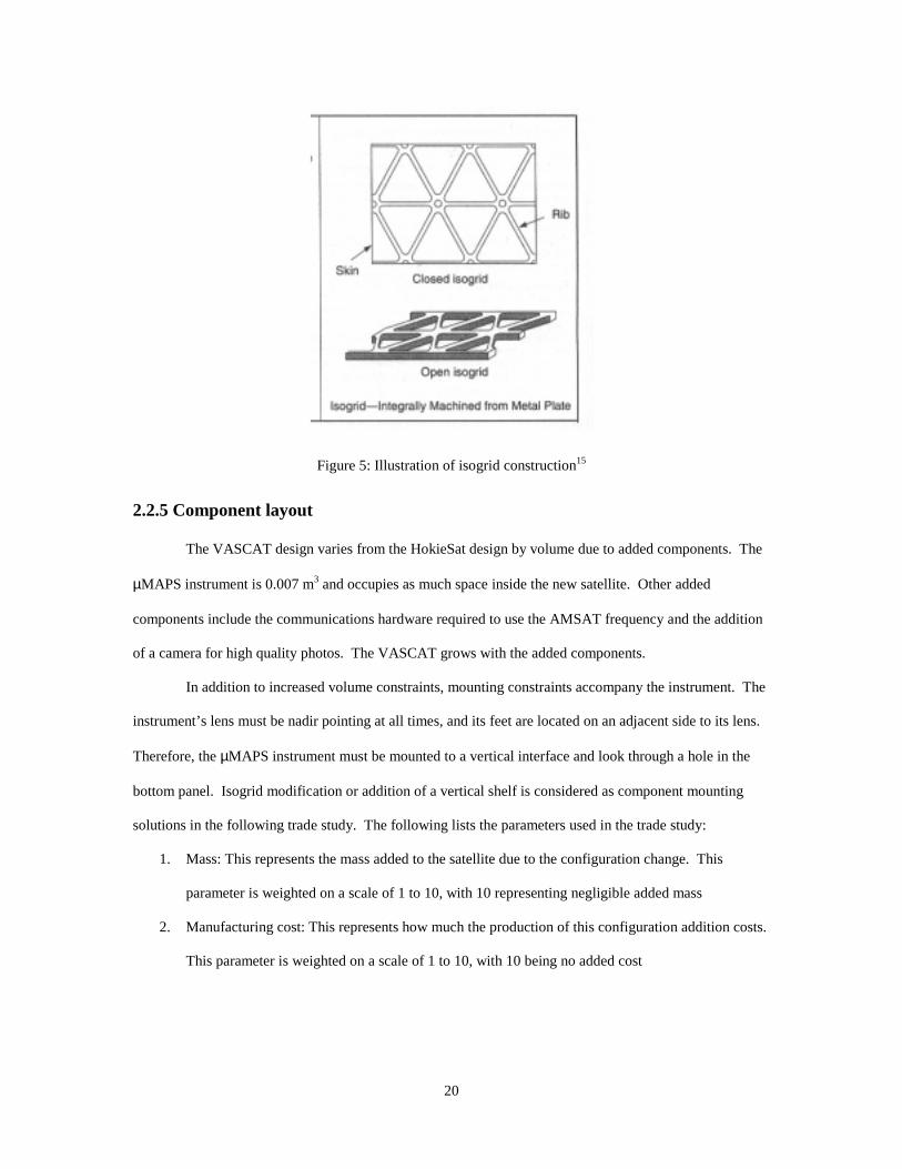
After all necessary structural analysis is performed to determine dimensions of the structure, the
type of structural configuration is chosen. Typically, increasing thickness increases buckling strength of a
structure. However, this directly conflicts with minimizing mass. A more effective way to strengthen and
stiffen a bus structure is to use isogrid construction. Isogrid consists of machining a plate of material into a
triangular pattern, as shown in Figure 5. This option is lighter than pure aluminum for smaller bus
structures, with identical strength properties in all load directions. 15 Because isogrid is the proposed
structure type, wall thickness must be increased to 3 mm to allow for ease in machining the isogrid,
adequate web strength, and a skin thick enough to support solar cells.
20
Figure 5: Illustration of isogrid construction15
2.2.5 Component layout
The VASCAT design varies from the HokieSat design by volume due to added components. The
µMAPS instrument is 0.007 m3 and occupies as much space inside the new satellite. Other added
components include the communications hardware required to use the AMSAT frequency and the addition
of a camera for high quality photos. The VASCAT grows with the added components.
In addition to increased volume constraints, mounting constraints accompany the instrument. The
instrument’s lens must be nadir pointing at all times, and its feet are located on an adjacent side to its lens.
Therefore, the µMAPS instrument must be mounted to a vertical interface and look through a hole in the
bottom panel. Isogrid modification or addition of a vertical shelf is considered as component mounting
solutions in the following trade study. The following lists the parameters used in the trade study:
1. Mass: This represents the mass added to the satellite due to the configuration change. This
parameter is weighted on a scale of 1 to 10, with 10 representing negligible added mass
2. Manufacturing cost: This represents how much the production of this configuration addition costs.
This parameter is weighted on a scale of 1 to 10, with 10 being no added cost
21
3. Ease in mounting: This represents a measure of how trivial attachment of components to the
structure will be. For example, threaded inserts are complicated while fasteners are fairly simple.
This parameter is weighted on a scale of 1 to 10, with 10 being the easiest to mount.
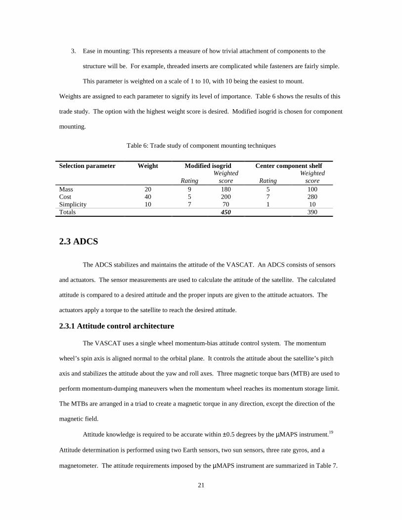
Weights are assigned to each parameter to signify its level of importance. Table 6 shows the results of this
trade study. The option with the highest weight score is desired. Modified isogrid is chosen for component
mounting.
Table 6: Trade study of component mounting techniques
Modified isogrid Center component shelf Selection parameter Weight
Rating Weighted
score Rating Weighted
score Mass 20 9 180 5 100 Cost 40 5 200 7 280 Simplicity 10 7 70 1 10 Totals 450 390
2.3 ADCS
The ADCS stabilizes and maintains the attitude of the VASCAT. An ADCS consists of sensors
and actuators. The sensor measurements are used to calculate the attitude of the satellite. The calculated
attitude is compared to a desired attitude and the proper inputs are given to the attitude actuators. The
actuators apply a torque to the satellite to reach the desired attitude.
2.3.1 Attitude control architecture
The VASCAT uses a single wheel momentum-bias attitude control system. The momentum
wheel’s spin axis is aligned normal to the orbital plane. It controls the attitude about the satellite’s pitch
axis and stabilizes the attitude about the yaw and roll axes. Three magnetic torque bars (MTB) are used to
perform momentum-dumping maneuvers when the momentum wheel reaches its momentum storage limit.
The MTBs are arranged in a triad to create a magnetic torque in any direction, except the direction of the
magnetic field.
Attitude knowledge is required to be accurate within ±0.5 degrees by the µMAPS instrument.19
Attitude determination is performed using two Earth sensors, two sun sensors, three rate gyros, and a
magnetometer. The attitude requirements imposed by the µMAPS instrument are summarized in Table 7.

22
Table 7: MicroMAPS imposed attitude requirements19
Requirement Value
Pointing Direction Nadir pointing Control accuracy (3σ) ± 2.5°
Knowledge accuracy (3σ) ± 0.5°
2.3.2 Attitude control modes
The VASCAT uses three modes of attitude control. The satellite operates in normal mode during
the majority of its mission. A momentum-dump mode is entered whenever the momentum wheel reaches
its upper limit of momentum storage. The satellite’s computer initiates safe mode should it experience
system level error.
2.3.2.1 Normal
The ADCS of the satellite operates in normal mode during the majority of its mission. The
attitude of the satellite is determined every ten seconds and transmitted to a ground station. All available
sensor data is used to determine attitude to ensure that the attitude knowledge is accurate to ±0.5 degrees.
Attitude knowledge is compared with the desired attitude and a control torque is applied using the
momentum wheel or magnetic torque bars accordingly. This ensures that the pointing error is kept below
±2.5 degrees.
2.3.2.2 Momentum-dump
The satellite uses a momentum wheel for attitude control and stabilization. Over time secular
attitude disturbances build up momentum in the wheel. When the build up of momentum reaches the
storage limit of the momentum wheel, a momentum-dumping maneuver is performed. The three MTBs are
used to apply an external torque to the satellite so that the momentum wheel applies an equal and opposite
torque to lower its spin rate. The attitude determination system performs as it does in normal mode, but the
magnetometer readings are not used for attitude determination while the MTBs are active.
2.3.2.3 Safe
The satellite enters safe mode if an error occurs during operation. The satellite’s computer
determines the entry and exit of this mode. During this mode the ADCS is passive. The momentum stored
in the momentum wheel and the gravity-gradient stabilize the satellite.

23
2.3.3 Disturbance torques
The VASCAT encounters disturbance torques on orbit. It is subjected to solar pressure, gravity-
gradient, atmospheric drag, and magnetic torques. A significant torque is due to the gravity-gradient. The
force of gravity varies with an object’s distance from the center of the Earth. The lower sections of the
satellite feel a greater gravitational force compared to the upper sections. The result is a torque exerted on
the satellite if it is not directly nadir pointing.
( )θµ2sin
2
33 yzg II
RT −=
2-920
The moments of inertia, Iz and Iy, of the satellite as well as its radius, R, and the angle off nadir, q,
determine the magnitude of the torque.
Solar pressure is exerted on the satellite by photons, emitted from the Sun, that strike the satellite.
The force is exerted at the center of solar pressure of the satellite. If the center of solar pressure and center
of gravity do not coincide then a torque is created.
( ) ( )cgciqAc
FT pssp
ssp −+= cos1
2-1020
The surface area exposed to the sun, Asp, the center of solar pressure, cps, the center of gravity, cg, and the
reflectance factor, q, are the satellite properties that determine the torque. The solar constant, Fs, and the
speed of light, c, are the constants that influence the magnitude of the torque.
The electronics on-board the VASCAT induce a magnetic dipole during operation. The magnetic
dipole interacts with the geomagnetic field to produce a torque. The maximum torque occurs when the
magnetic dipole direction is perpendicular to the geomagnetic field.
DBTm = 2-1120
The worst case magnitude of the torque is calculated using Equation 2-11, where D is the strength of the
magnetic dipole and B is the magnitude of the local geomagnetic field.
Although the atmosphere in Low-Earth Orbit (LEO) is sparse, the high velocity of a satellite
creates some drag. The drag force acts at the center of pressure of the satellite. If the center of pressure
does not coincide with the center of gravity, the drag creates a torque.

24
( )cgcAVCT pada −= 25.0 ρ 2-1220
The torque is equal to the drag force times the length of the moment arm, or the distance between
the center of atmospheric pressure, cpa, and the cg. Equation 2-12 is used to calculate the magnitude of the
torque, where ρ is the atmospheric density, Cd is the drag coefficient, A is the projected area, and V is the
velocity of the satellite.
Preliminary estimates of the structural properties and orbital parameters of the satellite are used to
estimate these torques. Table 8 summarizes the structural properties used in the calculations.
Table 8: Estimated structural properties of the VASCAT
Description Value Ix 4.4 kg/m2
Iy 4.4 kg/m2 Iz 1.9 kg/m2 As 0.18 m2 cg 0.10 m
c.p. 0.17 m Cd 2.5
The estimated orbital parameters used in the calculations for disturbance torques are summarized in
Table 9.
Table 9: Estimated orbital properties of the VASCAT
Description Value R 6778 km
ρ 2.72 × 10⁻¹² kg/m2
The disturbance torques are estimated using equations 2-9 through 2-12 above. A simple Matlab
code is used to perform the calculations, and is presented in Appendix D. Table 10 summarizes the results
of the calculations.

25
Table 10: Estimated disturbance torques
Disturbance Torque (N-m) Gravity gradient 4.8 × 10⁻⁶ Solar pressure 8.5 × 10⁻⁸
Magnetic 5.1 × 10⁻⁵ Atmospheric drag 2.3 × 10⁻¹²
The magnitude of the total disturbance torque is estimated to be 56 µN-m. The majority of the
disturbance torque is due to the magnetic torque created by the interaction of the satellite’s electronics with
the geomagnetic field. A magnetic dipole of 1 A-m2 was assumed for the magnetic disturbance torque
calculation. The second largest component is due to the gravity-gradient. The VASCAT is nadir pointing.
In this orientation the torque due to the gravity-gradient is zero and acts as a restoring torque in case of
deviation from nadir.
2.3.4 Hardware
The ADCS consist of two types of hardware: attitude sensors and attitude actuators. Attitude
sensors take measurements that determine the orientation of the satellite. Attitude actuators apply a torque
to the satellite to control its orientation.
2.3.4.1 Determination
The attitude determination hardware used by the VASCAT includes two Earth sensors, two sun
sensors, three rate gyros, and a magnetometer. Earth sensors are chosen as attitude sensors for the
VASCAT because it is an Earth-referenced satellite, and the sensors meet accuracy requirements. The
Earth sensors are Ithaco Conical Earth Sensors (CES). Figure 6 is a diagram of the sensor head of the CES
with dimensions.
26
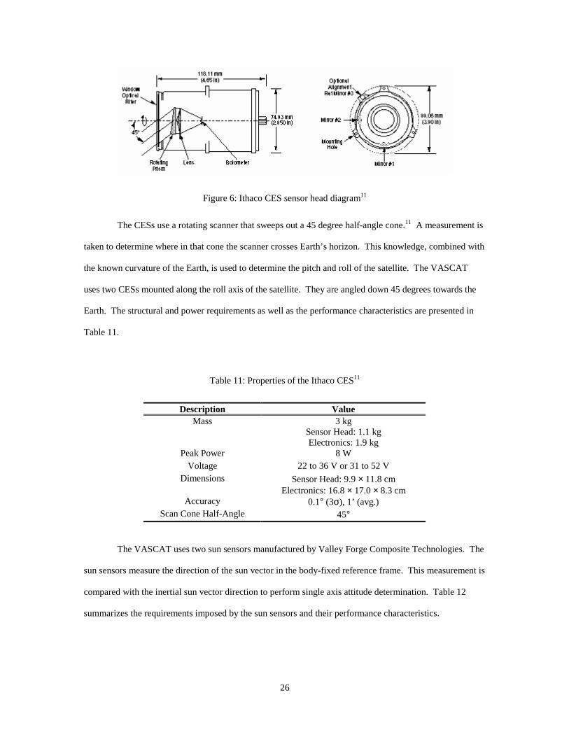
Figure 6: Ithaco CES sensor head diagram11
The CESs use a rotating scanner that sweeps out a 45 degree half-angle cone.11 A measurement is
taken to determine where in that cone the scanner crosses Earth’s horizon. This knowledge, combined with
the known curvature of the Earth, is used to determine the pitch and roll of the satellite. The VASCAT
uses two CESs mounted along the roll axis of the satellite. They are angled down 45 degrees towards the
Earth. The structural and power requirements as well as the performance characteristics are presented in
Table 11.
Table 11: Properties of the Ithaco CES11
Description Value Mass 3 kg
Sensor Head: 1.1 kg Electronics: 1.9 kg
Peak Power 8 W Voltage 22 to 36 V or 31 to 52 V
Dimensions Sensor Head: 9.9 × 11.8 cm Electronics: 16.8 × 17.0 × 8.3 cm
Accuracy 0.1° (3σ), 1’ (avg.) Scan Cone Half-Angle 45°
The VASCAT uses two sun sensors manufactured by Valley Forge Composite Technologies. The
sun sensors measure the direction of the sun vector in the body-fixed reference frame. This measurement is
compared with the inertial sun vector direction to perform single axis attitude determination. Table 12
summarizes the requirements imposed by the sun sensors and their performance characteristics.
27
Table 12: Properties of the Valley Forge Composite Technologies Sun Sensor18
Description Value Mass 350 grams
Peak Power 2.5 W Accuracy 1 arc second
Measurement Frequency 10 Hertz Field of View 100° × 50°
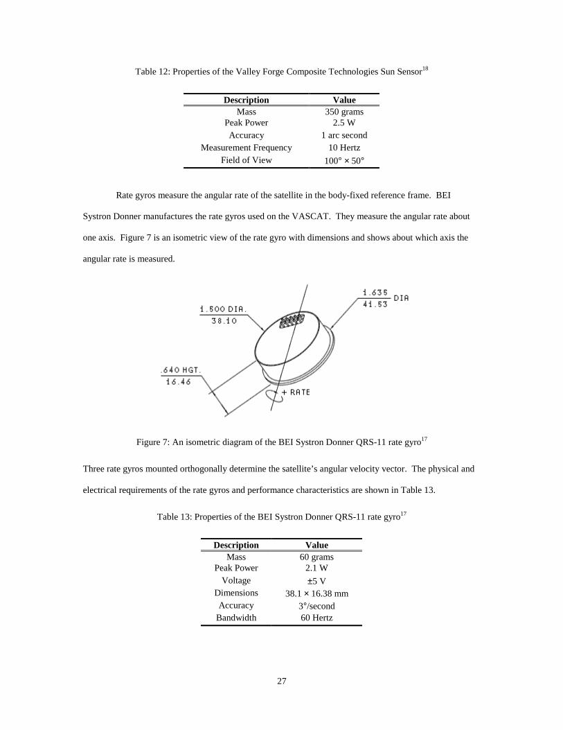
Rate gyros measure the angular rate of the satellite in the body-fixed reference frame. BEI
Systron Donner manufactures the rate gyros used on the VASCAT. They measure the angular rate about
one axis. Figure 7 is an isometric view of the rate gyro with dimensions and shows about which axis the
angular rate is measured.
Figure 7: An isometric diagram of the BEI Systron Donner QRS-11 rate gyro17
Three rate gyros mounted orthogonally determine the satellite’s angular velocity vector. The physical and
electrical requirements of the rate gyros and performance characteristics are shown in Table 13.
Table 13: Properties of the BEI Systron Donner QRS-11 rate gyro17
Description Value Mass 60 grams
Peak Power 2.1 W Voltage ±5 V
Dimensions 38.1 × 16.38 mm Accuracy 3°/second
Bandwidth 60 Hertz
28
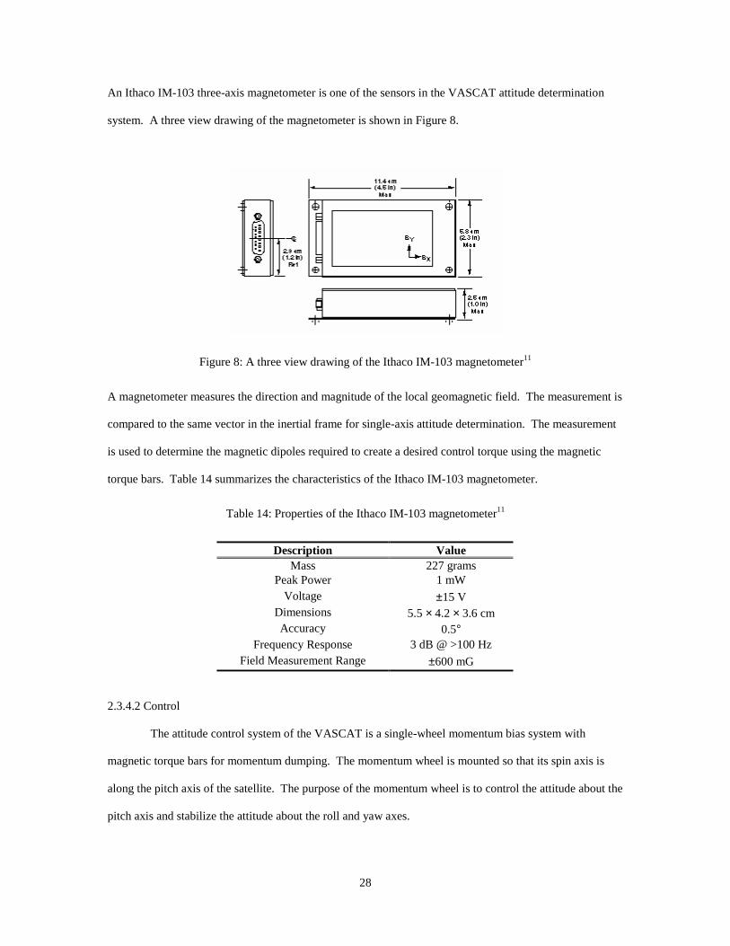
An Ithaco IM-103 three-axis magnetometer is one of the sensors in the VASCAT attitude determination
system. A three view drawing of the magnetometer is shown in Figure 8.
Figure 8: A three view drawing of the Ithaco IM-103 magnetometer11
A magnetometer measures the direction and magnitude of the local geomagnetic field. The measurement is
compared to the same vector in the inertial frame for single-axis attitude determination. The measurement
is used to determine the magnetic dipoles required to create a desired control torque using the magnetic
torque bars. Table 14 summarizes the characteristics of the Ithaco IM-103 magnetometer.
Table 14: Properties of the Ithaco IM-103 magnetometer11
Description Value Mass 227 grams
Peak Power 1 mW Voltage ±15 V
Dimensions 5.5 × 4.2 × 3.6 cm Accuracy 0.5°
Frequency Response 3 dB @ >100 Hz Field Measurement Range ±600 mG
2.3.4.2 Control
The attitude control system of the VASCAT is a single-wheel momentum bias system with
magnetic torque bars for momentum dumping. The momentum wheel is mounted so that its spin axis is
along the pitch axis of the satellite. The purpose of the momentum wheel is to control the attitude about the
pitch axis and stabilize the attitude about the roll and yaw axes.

29
The sizing of the momentum wheel is based on the maximum disturbance torque applied to the
satellite, and the accuracy requirement of ±2.5 degrees. The reaction torque capability must cope with the
maximum total disturbance torque, estimated to be 56 µN-m. The amount of stability required by the
satellite and the maximum disturbance torque determines the momentum capacity of the momentum wheel.
µπ
θ
3
2
aTh
a
D= 2-1320
The disturbance torque, TD, the semi-major axis of the orbit, a, and the allowable angular deviation, θa,
affect the required momentum storage capability. 20 The calculations are performed using the values shown
in Table 15. The momentum wheel is required to maintain 1.78 N-m-s of momentum.
Table 15: VASCAT orbital and environmental properties
Description Symbol Value Semi-major axis a 6778 km
Disturbance torque TD 56 µN-m Allowable angular deviation θa ±2.5°
The momentum wheel used in the VASCAT is an Ithaco TW-4A12 momentum wheel. Figure 9 is
a cut-away diagram depicting the internal configuration of this momentum wheel.
Figure 9: A cut-away diagram showing the interior of an Ithaco Type A momentum wheel11
This momentum wheel is capable of 12 mN-m of torque, which exceeds the maximum disturbance
torque of 56 µN-m. The maximum momentum capacity of the wheel is 4 N-m-s.11 The momentum wheel

30
operates with at least 2 N-m-s of momentum stored at all times to satisfy the stability requirement. The
mass and power properties and performance characteristics of the momentum wheel are summarized in
Table 16.
Table 16: Properties of the Ithaco TW-4A12 momentum wheel11
Description Value Mass 3.46 kg
Motor Drive: 2.55 kg Wheel: 0.91 kg
Peak Power 25 W Dimensions Motor Drive: 15 × 19 × 32 cm
Wheel: 20.5 × 6.4 cm Momentum Capacity 4 N-m-s
Reaction Torque 12 mN-m Steady State Power Max. Speed: 9 W
@ 1000 rpm: 5 W Speed Range ±5100 rpm
Momentum dumping is performed using magnetic torque bars (MTBs). Magnetic torque bars
induce a magnetic dipole that interacts with the geomagnetic field to create a torque on the satellite. 20 The
MTBs are mounted orthogonally. This arrangement allows greater flexibility in inducing the direction of
the magnetic dipole.
The MTBs are sized to provide sufficient torque to dump enough of the momentum wheel’s
momentum within a reasonable amount of time. The maximum storage capacity of the momentum wheel is
4 N-m-s, and the minimum storage capacity required for attitude stabilization is 2 N-m-s. Therefore, a
momentum-dumping maneuver is required whenever 2 N-m-s of momentum is built up in the wheel. The
amount of added momentum stored in the wheel during a single orbit is calculated using the following
equation.
µπ
3
2a
Th D= 2-1420
The momentum stored per orbit is 0.22 N-m-s. Approximately every 9 orbits a momentum-dumping
maneuver is required. The maneuver for the VASCAT takes approximately 22 minutes. The torque
required to accomplish this is 1.52 mN-m. The magnetic dipole necessary to meet the torque requirement
is the magnitude of the torque divided by the magnitude of local magnetic field.17 The magnitude of the
31
local magnetic field is assumed to be 4.5 × 10⁻⁵ Tesla in the worst case. Using the worst case results in a
required magnetic dipole of 33.67 A-m2.
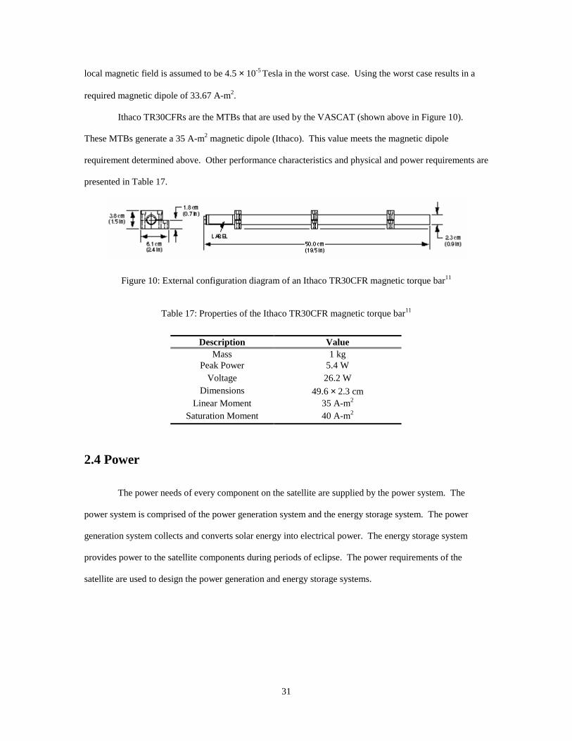
Ithaco TR30CFRs are the MTBs that are used by the VASCAT (shown above in Figure 10).
These MTBs generate a 35 A-m2 magnetic dipole (Ithaco). This value meets the magnetic dipole
requirement determined above. Other performance characteristics and physical and power requirements are
presented in Table 17.
Figure 10: External configuration diagram of an Ithaco TR30CFR magnetic torque bar11
Table 17: Properties of the Ithaco TR30CFR magnetic torque bar11
Description Value Mass 1 kg
Peak Power 5.4 W Voltage 26.2 W
Dimensions 49.6 × 2.3 cm Linear Moment 35 A-m2
Saturation Moment 40 A-m2
2.4 Power
The power needs of every component on the satellite are supplied by the power system. The
power system is comprised of the power generation system and the energy storage system. The power
generation system collects and converts solar energy into electrical power. The energy storage system
provides power to the satellite components during periods of eclipse. The power requirements of the
satellite are used to design the power generation and energy storage systems.

32
2.4.1 Power Requirements
The components on the VASCAT require conditioned electrical power to function. Each
component has a specific power and voltage requirement. The power system must meet the needs of all the
satellite components. Table 18 is a list of all the satellite components and their power requirements.
Table 18: Component power requirements
System Device Average power(W) Peak power(W) Voltages (V)
Comm: Uplink 1.5 3 28 Downlink 3 5 28 AMSAT 1.8 2 28 Dual single board computer 3.5 4 28 ADCS: Momentum Wheel 9 25 28 Magnet Torque Bars 4.2 5.4 28 Magnetometer 0.0008 0.001 28 Magnetometer Board 0.036 0.037 28 Earth Sensors 5 8 28 Earth Sensor board 0.12 0.6 28 Sun Sensor 2 2.5 28 Rate Gyro 1.5 2.1 28 MT and RG Board 0.5 0.8 28 UMAPS: Calibrate 27.2 27.2 28 Normal Operation 16.2 16.2 28 GN&C: GPS 3 5 28 Camera: Camera 3 3.5 28
The power system is modeled from the peak power requirements to ensure that it supplies enough
power to the satellite. A power budget quantifies the amount of power required for a single orbit, and it
shows which components operate during daylight and eclipse. If the power system provides enough power
to fulfill the budget for peak power needs, it is sufficient for all other cases. The VASCAT runs off of a
28 V bus voltage.

33
Table 19: Daylight and eclipse power budget
Daylight Eclipse
Operation: Power
(W) Duration (s) Energy (W-s) Duration (s) Energy (W-s) Uplink 3 600 1,800 0 0 Downlink 5 600 3,000 0 0 AMSAT 2 3,500 7,000 2,150 4,300 Dual single board computer 4 3,500 14,000 2,150 8,600 Momentum Wheel 25 3,500 225 2,150 19,350 Magnet Torque Bars 5.4 3,500 6,480 0 0 Magnetometer 0.001 3,500 3.5 2,150 2 Magnetometer Board 0.037 3,500 128 2,150 79 Earth Sensors 8 3,500 28,000 2,150 17,200 Earth Sensor board 0.6 3,500 2,100 2,150 1,290 Sun Sensor 2.5 3,500 8,740 2,150 5,370 Rate Gyro 2.1 3,500 7,340 2,150 4,510 MT and RG Board 0.5 3,500 1,750 2,150 1,075 Calibrate 27.2 120 3,260 0 0 Normal Operation 16.2 3,500 56,600 2,150 34,820 GPS 5 3,500 17,500 2,150 10,750 Camera 3 3,500 10,500 0 0
Table 19 is a power budget of all the components showing the peak power, duration of operation,
and energy during daylight and eclipse. These power requirements are used to design power generation
and energy storage systems.
2.4.2 Power Generation
The power generation components fulfill the daylight power budget and adequately charge the
energy storage system. Power generation system options include fuel cells, radio-isotope thermoelectric
generators (RTG), and solar arrays. Fuel cells are not used for the VASCAT because of their relatively
short lifetimes. Radio-isotope thermoelectric generators are too large and politically impractical because of
their radioactive contents. VASCAT uses arrays of solar cells that convert solar energy from the sun into
electrical energy. This method of power generation has extensive space heritage. Solar-to-electric energy
conversion is a beneficial method of power generation for the VASCAT because solar energy is an
inexhaustible resource and is easily harnessed. The amount of energy the VASCAT receives from the sun
remains relatively constant over the 3 year lifetime.
The efficiency of solar cells degrades over time due to prolonged exposure to solar radiation. The
severity of the lifetime degradation is different for each type of solar cell. These effects range from two to
34
four percent of the power produced each year. The VASCAT uses a Gallium Arsenide, single-junction
solar cell made by Spectrolab with low lifetime degradation of three percent. They convert solar energy
into electrical energy at an electric potential of around 0.9 V.16
The VASCAT’s power requirements make body-mounted solar cells a feasible option. The solar
cells are connected in series to produce the required 28 V bus voltage. There are 11 strings total on the side
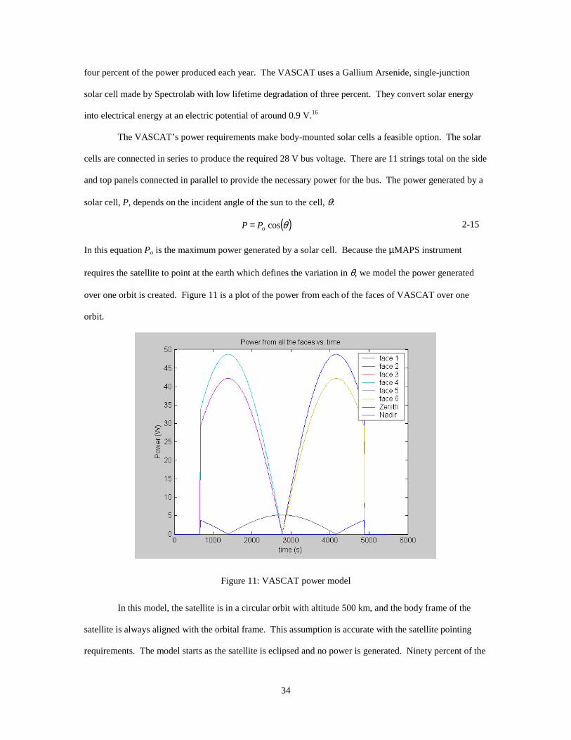
and top panels connected in parallel to provide the necessary power for the bus. The power generated by a
solar cell, P, depends on the incident angle of the sun to the cell, θ:
( )θcosoPP = 2-15
In this equation Po is the maximum power generated by a solar cell. Because the µMAPS instrument
requires the satellite to point at the earth which defines the variation in θ, we model the power generated
over one orbit is created. Figure 11 is a plot of the power from each of the faces of VASCAT over one
orbit.
Figure 11: VASCAT power model
In this model, the satellite is in a circular orbit with altitude 500 km, and the body frame of the
satellite is always aligned with the orbital frame. This assumption is accurate with the satellite pointing
requirements. The model starts as the satellite is eclipsed and no power is generated. Ninety percent of the
35
side panel area and 10% of the zenith and nadir area is covered with solar cells. This configuration
accounts for the minimum power generated halfway through the orbit as the satellite eclipses Earth, and the
zenith surface is facing the sun. The model runs for the maximum off-nadir attitude for the instrument to
ensure that the power system meets the needs of the satellite in any normal operation orbit.
2.4.3 Energy Storage
The energy storage system must provide all the power needs of the satellite components during
eclipse. The amount of power needed from this system is determined from the power budget and the orbit.
The eclipse power budget, shown in Table 19, gives the power needs of the components. The orbit
determines the duration that the energy storage system needs to provide that power.
The VASCAT uses batteries for energy storage. Batteries have high energy densities and
extensive space heritage. Battery life decreases with the amount that the battery is discharged and is
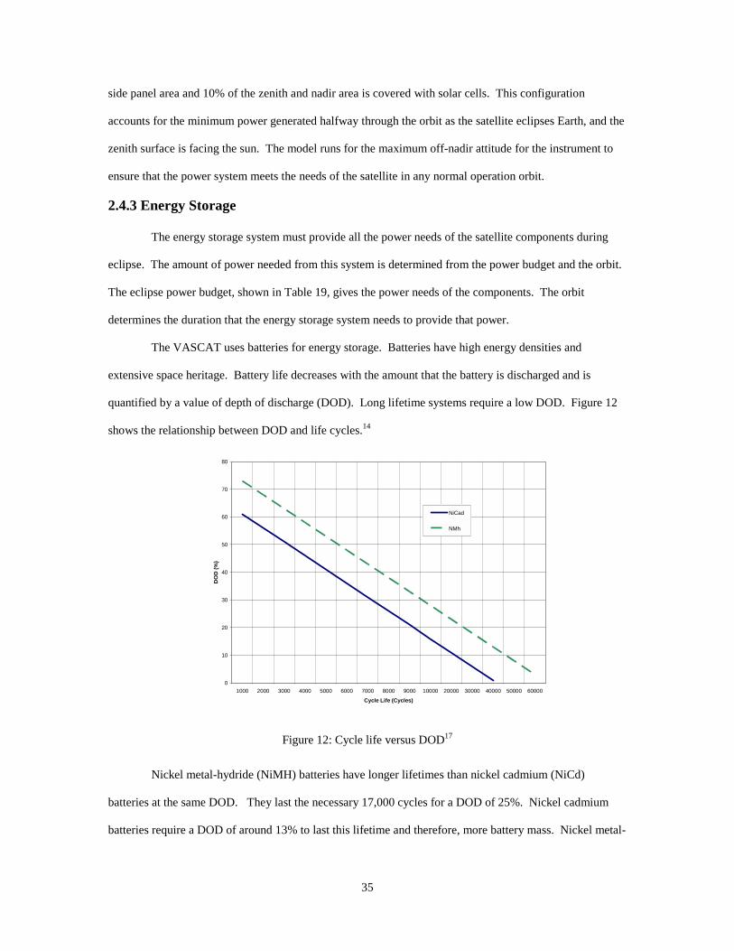
quantified by a value of depth of discharge (DOD). Long lifetime systems require a low DOD. Figure 12
shows the relationship between DOD and life cycles.14
0
10
20
30
40
50
60
70
80
1000 2000 3000 4000 5000 6000 7000 8000 9000 10000 20000 30000 40000 50000 60000
Cycle Life (Cycles)
DO
D (
%)
NiCad
NMh
Figure 12: Cycle life versus DOD17
Nickel metal-hydride (NiMH) batteries have longer lifetimes than nickel cadmium (NiCd)
batteries at the same DOD. They last the necessary 17,000 cycles for a DOD of 25%. Nickel cadmium
batteries require a DOD of around 13% to last this lifetime and therefore, more battery mass. Nickel metal-

36
hydride batteries are chosen for the VASCAT. The battery cells chosen are produced by Sanyo (HR-
4/3FAU 4500).
Summing the energy column in Table 19 gives the total energy the VASCAT needs each eclipse
period:
mcDODE
EN
d
ec ⋅⋅
= 2-1620
Equation 2-16 calculates the number of cells needed in the battery box, where Nc is the number of cells, Ee
is the eclipse energy, Ed is the energy density of the batteries, and mc is the mass of one battery.
Calculations yield a NiMH cell that is approximately 62 g. The battery box holds 24 1.2V cells, connected
in series and regulated by a control system to provide the 28 V bus voltage.
2.5 Thermal
The thermal subsystem of the VASCAT keeps all components within their operational
temperature limits. A thermal control system (TCS) achieves this goal as efficiently as possible by
minimizing power consumption, complexity, and mass. A passive TCS, which requires no power or
control, is the best solution to minimize these criteria.
A preliminary thermal analysis determines the temperature variations the satellite experiences on
orbit. This analysis is presented in Table 20. It assumes a spherical satellite with uniform surface
properties. The minimum and maximum power dissipations are estimates from the preliminary power
budget. The other values presented are discussed in more detail later in this section chapter.
37
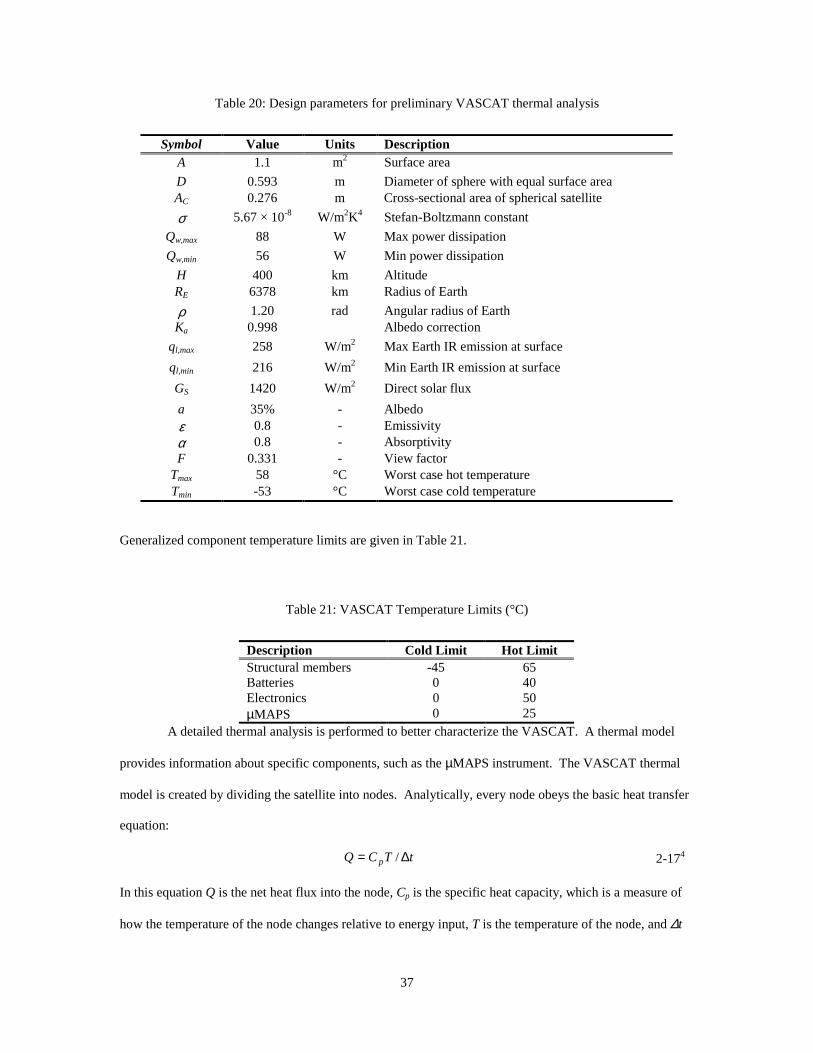
Table 20: Design parameters for preliminary VASCAT thermal analysis
Symbol Value Units Description A 1.1 m2 Surface area
D 0.593 m Diameter of sphere with equal surface area AC 0.276 m Cross-sectional area of spherical satellite
σ 5.67 × 10⁻⁸ W/m2K4 Stefan-Boltzmann constant
Qw,max 88 W Max power dissipation
Qw,min 56 W Min power dissipation
H 400 km Altitude RE 6378 km Radius of Earth
ρ 1.20 rad Angular radius of Earth Ka 0.998 Albedo correction
ql,max 258 W/m2 Max Earth IR emission at surface
ql,min 216 W/m2 Min Earth IR emission at surface
GS 1420 W/m2 Direct solar flux
a 35% - Albedo ε 0.8 - Emissivity α 0.8 - Absorptivity F 0.331 - View factor
Tmax 58 °C Worst case hot temperature Tmin -53 °C Worst case cold temperature
Generalized component temperature limits are given in Table 21.
Table 21: VASCAT Temperature Limits (°C)
Description Cold Limit Hot Limit Structural members -45 65 Batteries 0 40 Electronics 0 50 µMAPS 0 25
A detailed thermal analysis is performed to better characterize the VASCAT. A thermal model
provides information about specific components, such as the µMAPS instrument. The VASCAT thermal
model is created by dividing the satellite into nodes. Analytically, every node obeys the basic heat transfer
equation:
tTCQ p ∆= / 2-174
In this equation Q is the net heat flux into the node, Cp is the specific heat capacity, which is a measure of
how the temperature of the node changes relative to energy input, T is the temperature of the node, and ∆t
38
is change in time. This equation is solved for the temperature of the node if the heat flux is known. Each
pertinent component, as well as the bus structure side panels, is assigned to a node. The specific heat of
each node is calculated by multiplying the component mass by the specific thermal capacitance of its
primary material (typically aluminum).
Nodes transfer heat between themselves by conduction. Conduction couplings are a measure of
how a node transfers heat to another node that is touching it. The following equation is the governing
conduction heat transfer equation:
( )Tl
kAQcond ∆= 2-184
The kA/L term is the conduction coupling value, G, in W/K. As shown, G is a function of the contact area
between nodes, A, the heat path length, l, and the material thermal conductivity, k. The conduction
couplings are calculated using the geometry of the satellite and knowledge of the materials used.
Radiation heat exchange takes place between nodes and space. For the purposes of this analysis,
internal radiation between components is neglected. The internal surfaces of the satellite are painted black,
which minimizes internal radiative heat transfer. Only radiation from the bus external surfaces to space is
considered. Radiation heat transfer is given by:
( )44spacenoderad TTAQ −= σε 2-194
In this equation A is the surface area, σ is the Steffan-Boltzmann constant, and ε is the emissivity of the
surface. The emissivity of the node is determined from the properties of its thermal coating, and the
surface area is found from geometry.
Generation of a thermal model requires knowledge of the heat fluxes (see Equation 2-17) in
addition to the heat transfer paths. Nodal heat fluxes are determined from the internal component
dissipations and environmental inputs. Hot and cold cases are considered. The hot case includes the
maximum or peak power dissipations from each of the components and the maximum orbit averaged fluxes
on the satellite. Likewise, the cold case includes the minimum operational power dissipations and the
minimum orbit averaged fluxes.
The internal dissipations are determined by the mission operation requirements and are obtained
from the power subsystem. The component dissipations used for each of the cases are given in Table 22.

39
Table 22: Component internal power dissipations
Total power (W) Description Hot Cold
µMAPS 27.2 16.2 Momentum Wheel 25 7 Magnetic Torque Bars 16.2 12.6 Magnetometer 0.001 0.0008 Earth Sensors 16 16 Sun Sensors 5 5 Rate Gyros 6.3 6.3
The orbit averaged fluxes are calculated from information about the satellite’s orbit. The external heat
sources are direct solar energy, Earth infrared (IR) and albedo. Albedo is a measure of how much of the
sun’s energy is reflected from the Earth’s atmosphere and surface back into space, and is usually given as a
percentage.6 The cold case analysis assumes the satellite is in eclipse and the only external heat source is
from the Earth. The environmental fluxes are shown in Table 23.
Table 23: Environmental fluxes in space (W/m2)
Source Hot Cold Solar 1418 0 Earth IR 258 216 Albedo 35% 25% Totals 2172.3 216
The actual heat input depends on the surface properties of the satellite. Absorbtivity, α, is a
measure of how much external radiation is absorbed by the surface in question and is dependant upon the
thermal coating applied. Emissivity characterizes how much heat the surface radiates according to
Equation 2-19.20 The surface properties of various VASCAT external components are given in Table 24.6
Table 24: Surface properties
Component Coating / Material αααα εεεε Side Panels Silicon 0.8 0.8 Nadir Panel White Paint 0.3 0.9 Solar arrays White Paint 0.3 0.9
40
The total input power is determined by:
( )sexternal GAQ ℑ= α 2-20
In this equation the term in parenthesis is the total orbit average flux in W/m2. View factor, ℑ , describes
how the surface is oriented relative to the flux vector.
View factor is a parameter that varies depending upon the position of the satellite relative to the
orbital frame. For example, the nadir panel of the satellite is Earth-pointing, and therefore rarely has a full
view of the sun. Therefore, the nadir panel view factor is approximately 0.2. The view factor is
determined by the MATLAB code in Appendix A. This code determines the power output from body-
mounted solar cells on a hexagonal cylinder at various positions in an orbit. It outputs the projected area
that a surface will ‘see’ relative to the solar vector. This projected area is then used to determine the view
factor for the external bus surfaces.
The thermal model is assembled after the heat transfer paths are identified and internal and
external heat sources are considered. The thermal analysis requires simultaneous evaluation of Equations
2-17, 2-18, and 2-19 at each node. This evaluation is complex due to the nonlinear relationship between
the temperature of a node and its resulting heat flux.9
The Systems Integrated Numerical Differential Analyzer (SINDA), a thermal analysis package
commonly used in industry, analyzes the VASCAT thermal model.3 This software package calculates
nodal temperatures based on user-generated conduction and radiation couplings and input fluxes. The
program then uses an explicit forward solution method to evaluate the governing heat transfer equations.
The explicit forward method uses the conditions at the current time step, or iterative loop, to calculate the
temperature of each of the nodes in the system. It then performs an energy balance check on each of the
nodes and varies the time step accordingly. The result is a steady state solution for nodal temperatures.
The µMAPS instrument is the mission driver for the VASCAT, so several steps are taken to
thermally control it. The instrument is conductively coupled to the nadir and zenith panels of the satellite.
Additionally, the nadir and zenith panels are coated with white paint to increase their dissipation to space
and reduce their incident heat flux.
The hot and cold case temperatures of the VASCAT components are listed in Table 25. Almost
all component temperatures are within their specified limits. The exception is the µMAPS instrument. In
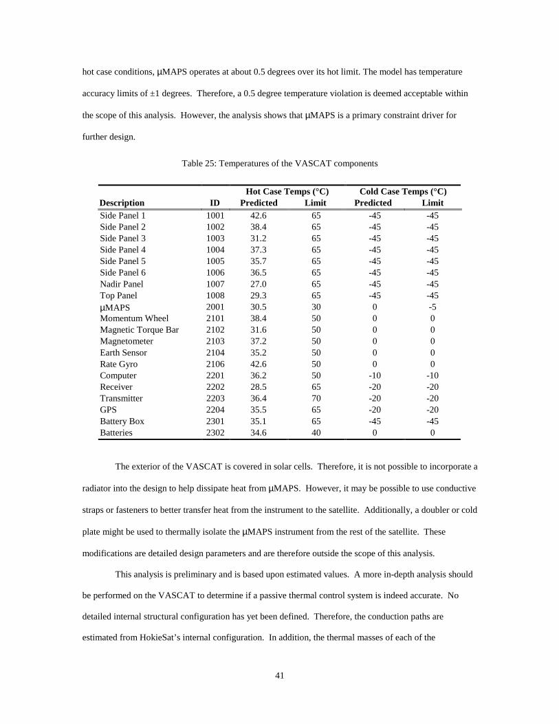
41
hot case conditions, µMAPS operates at about 0.5 degrees over its hot limit. The model has temperature
accuracy limits of ±1 degrees. Therefore, a 0.5 degree temperature violation is deemed acceptable within
the scope of this analysis. However, the analysis shows that µMAPS is a primary constraint driver for
further design.
Table 25: Temperatures of the VASCAT components
Hot Case Temps (°C) Cold Case Temps (°C) Description ID Predicted Limit Predicted Limit Side Panel 1 1001 42.6 65 -45 -45 Side Panel 2 1002 38.4 65 -45 -45 Side Panel 3 1003 31.2 65 -45 -45 Side Panel 4 1004 37.3 65 -45 -45 Side Panel 5 1005 35.7 65 -45 -45 Side Panel 6 1006 36.5 65 -45 -45 Nadir Panel 1007 27.0 65 -45 -45 Top Panel 1008 29.3 65 -45 -45 µMAPS 2001 30.5 30 0 -5 Momentum Wheel 2101 38.4 50 0 0 Magnetic Torque Bar 2102 31.6 50 0 0 Magnetometer 2103 37.2 50 0 0 Earth Sensor 2104 35.2 50 0 0 Rate Gyro 2106 42.6 50 0 0 Computer 2201 36.2 50 -10 -10 Receiver 2202 28.5 65 -20 -20 Transmitter 2203 36.4 70 -20 -20 GPS 2204 35.5 65 -20 -20 Battery Box 2301 35.1 65 -45 -45 Batteries 2302 34.6 40 0 0
The exterior of the VASCAT is covered in solar cells. Therefore, it is not possible to incorporate a
radiator into the design to help dissipate heat from µMAPS. However, it may be possible to use conductive
straps or fasteners to better transfer heat from the instrument to the satellite. Additionally, a doubler or cold
plate might be used to thermally isolate the µMAPS instrument from the rest of the satellite. These
modifications are detailed design parameters and are therefore outside the scope of this analysis.
This analysis is preliminary and is based upon estimated values. A more in-depth analysis should
be performed on the VASCAT to determine if a passive thermal control system is indeed accurate. No
detailed internal structural configuration has yet been defined. Therefore, the conduction paths are
estimated from HokieSat’s internal configuration. In addition, the thermal masses of each of the
42
components are estimates. Finally, a transient analysis, which takes into account the change in variations in
temperature of the satellite over the course of an orbit, should be performed to ensure that a passive TCS is
adequate.
2.6 Communication
The communications system of the VASCAT transmits telemetry and health information to a
ground station and receives commands from a ground station. The VASCAT communications system is
based on HokieSat’s communications system with the addition of an AMSAT link.
2.6.1 Uplink
The uplink portion of the communications system operates at approximately 450 MHz using a
loop antenna with a 100KHz bandwidth. The loop antenna is a HokieSat custom design, as shown in
Appendix B. The loop antenna is mounted on the nadir panel of the satellite and is connected to an ultra-
high frequency (UHF) receiver. The uplink system receives commands from ground stations.5
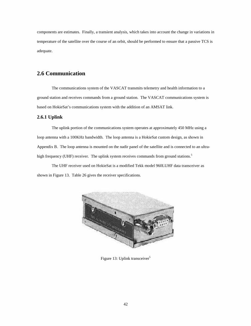
The UHF receiver used on HokieSat is a modified Tekk model 960LUHF data transceiver as
shown in Figure 13. Table 26 gives the receiver specifications.
Figure 13: Uplink transceiver5
43
Table 26: Uplink receiver specifications5
Type Value
FCC ID GOXKS-900/15.22.90
Frequency 430-450MHz
Operating Temperature -30 to +60°C
Voltage 9.6 V
Dimensions 3.4” × 2.1” × 0.9”
Weight 5.2 ounces
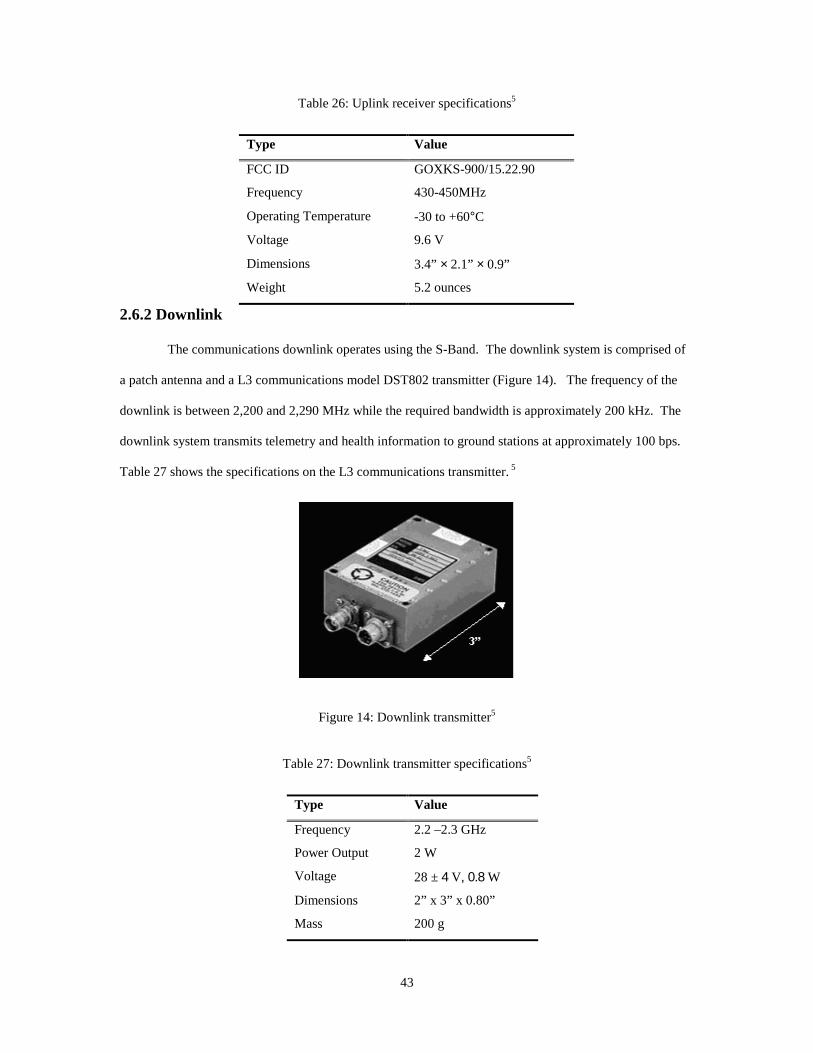
2.6.2 Downlink
The communications downlink operates using the S-Band. The downlink system is comprised of
a patch antenna and a L3 communications model DST802 transmitter (Figure 14). The frequency of the
downlink is between 2,200 and 2,290 MHz while the required bandwidth is approximately 200 kHz. The
downlink system transmits telemetry and health information to ground stations at approximately 100 bps.
Table 27 shows the specifications on the L3 communications transmitter. 5
Figure 14: Downlink transmitter5
Table 27: Downlink transmitter specifications5
Type Value
Frequency 2.2 –2.3 GHz
Power Output 2 W
Voltage 28 ± 4 V, 0.8 W
Dimensions 2” x 3” x 0.80”
Mass 200 g

44
2.6.3 AMSAT
The AMSAT link of the communications system transmits the data produced by the µMAPS
instrument. The µMAPS instrument produces 40 bps of data. Every ten seconds the µMAPS instrument
requires a time stamp, attitude, position, and velocity of the VASCAT added to the data to be downloaded.
Assuming that the satellite data is available as floats, a total of 35.2 bps is added to the link budget. With
the addition of the satellite data, the AMSAT link needs to transmit a total of 75.2 bps.19
The UoSAT-OSCAR 22 and the Malaysian-OSCAR 46 spacecraft use the AMSAT as their
primary downlink to ground stations. These spacecraft have the capability of a 9,600 bps download rate
using a transmitter at 435.12 MHz. The UoSAT-OSCAR 22 spacecraft uses the AMSAT to send grayscale
pictures of the earth down to the ground stations. The size of the OSCAR 22 pictures is approximately
109 bytes.2 If VASCAT uses the same method and size for pictures of the Earth's atmosphere, a picture
could be downloaded in 10 seconds using the maximum 9,600 bps download rate. The requirements on the
AMSAT portion of the communications system needs to be defined further before the specific hardware is
selected for use in the VASCAT satellite.
2.7 Command and data handling
The command and data handling system of the VASCAT satellite is identical to the HokieSat
system. The computer is centered on a Hitachi SuperH RISC Processor, with a 16 MB telemetry buffer, a
digital and analog interface subsystem, and a DMA-oriented CMOS camera frame buffer. The orbit
average power is 3 W for the computer which. The computer can handle approximately 20 million
instructions per second and is radiation hardened to 5 krads. The computer uses VxWorks as a real-time
operating system.12
2.8 Summary
Chapter two presents the preliminary subsystem designs and configuration for the VASCAT. The
systems defined in this chapter include the structure, the ADCS, the power system, the thermal system and
the communications system. Each system is developed based on the HokieSat design. The designs
presented in Chapter 2 serve as a starting point for further research and development.

45
Chapter 3: Mission Operations
3.1 Orbits
The main parameters considered in choosing the VASCAT orbit include the amount of Earth
coverage the orbit pattern can provide and the lifetime of the satellite in its given orbit. The sensitivity of
the µMAPS instrument requires a satellite without a propulsion system. The lack of a propulsion system
also reduces the complexity of the satellite and reduces operations costs. The success of the mission
depends heavily on the satellite’s ability to sustain a three-year lifetime without propulsion. This chapter
presents analysis done to determine Earth ground coverage and lifetime predictions.
3.1.1 Coverage
The objective of the µMAPS instrument is to perform analysis on samples of the Earth’s
atmosphere. Using the maximum amount of points possible in the Earth’s atmosphere is important to the
success of the mission. Each one of these points corresponds to a point on the Earth’s surface. Using
MATLAB, a coverage analysis is designed to determine the amount of time the µMAPS instrument sees
each of these points over a given satellite lifetime. This code is shown in Appendix C.
The MATLAB code uses inputs of the five main orbital parameters: semi-major axis, eccentricity,
inclination, argument of perigee, and right ascension of ascending node. It begins by defining a 91 × 361
coverage matrix whose components are all initially zero. The components of this matrix correspond to
each point of latitude and longitude on the Earth’s surface. Based on the assumption that the northern and
southern hemispheres have symmetrical coverage patterns, only 90 degrees of latitude are used. The
program first propagates the input orbit over a given lifetime, in steps of mean motion, to determine the
position and velocity of the satellite at any given time during the precession. For each point in time, the
code then iterates through a series of targets, each corresponding to one point on the Earth’s surface. These
targets cover each point over 90º of latitude and 360º of longitude. The Earth center angle (ECA) is
calculated between the satellite and the target and is compared with the angle associated with the field of
view of the instrument. The field of view of the instrument is 3º, or approximately 25 km2 on the surface of
the Earth.19 If the ECA is greater than the field of view, the satellite is not in view of its target. If the ECA

46
is less than the field of view, then the target is in view and that element of the coverage matrix is
incremented by one to show that the target has been viewed for one second. This code iterates over a
period of 100 orbits. After 100 orbits, the orbit pattern repeats. Therefore, the coverage over the entire
lifetime of the satellite is determined. Parameters such as orbit inclination and altitude alter the range and
frequency of coverage. This code is used to compare the coverage of a series of orbits. This orbit property
is considered along with other factors to determine the optimal orbit for the VASCAT. This type of data is
also used as a concrete model illustrating the capabilities of the mission.
3.1.2 Orbit prediction
Lifetime calculations predict the amount of time a LEO satellite remains in orbit before
atmospheric drag causes re-entry. The lifetime of a satellite is calculated to decide if the mission goals are
fulfilled before end-of-life, and determine optimal orbit parameters. Sources of uncertainty in satellite
orbital lifetime prediction are estimated future solar radio flux and geomagnetic activity, modeled
atmospheric density, and ballistic factor. The main source of uncertainty in models estimating future
atmospheric density at orbital altitude is the solar extreme ultraviolet heat input values. An important
problem in mission planning and satellite command & control is accurate prediction of orbital motion.
3.1.3 Orbit simulation
An orbit propagator is a mathematical algorithm for predicting the future position and velocity (or
orbital elements) of an orbit given some initial conditions and assumptions. There are a wide variety of
orbit propagation techniques available with different accuracy and applications. All built-in assumptions
must be known before deciding on a propagation scheme.
An accurate atmospheric model computes drag effects using Satellite Tool Kit’s (STK) lifetime
prediction feature.1 The gravitational model for the Earth is significantly simplified since the inclusion of
the higher order terms does not impact orbit decay estimates.
3.1.4 Orbit characteristics
The VASCAT launches into a circular orbit with an initial altitude of 450 km and an inclination of
57 degrees. The desired design lifetime of the satellite is initially three years. A circular orbit obtains
homogeneous and complete global coverage of the Earth. An initial altitude of 450 km guarantees a multi-

47
year mission duration even under severe solar activity conditions. The altitude decreases over the mission
lifetime due to atmospheric drag. The VASCAT may pass through the solar activity maximum, depending
on launch. The predicted natural decay depends on the magnitude of the actual solar activity cycle.
3.1.5 Lifetime
The lifetime tool, available in STK, is used to estimate the amount of time the VASCAT remains
in orbit. Lifetime computations are based on complex orbital theory and an accurate environment model.
The results are only an estimate. Due to variations in atmospheric density and irregular solar activity,
satellite lifetimes are determined with accuracy no better than ±10 %.1 To implement a practical computer
lifetime program, some assumptions and simplifications are made that add additional degrees of uncertainty
to the final result. Various parameters that effect lifetime include mass, altitude, satellite drag coefficient,
satellite drag area, and orbit inclination. Because the VASCAT’s mass is fixed at approximately the
35-50 kg margin, all calculations are performed with the satellite’s mass fixed at 50 kg.
The most important parameter in determining the lifetime of the VASCAT is initial altitude.
Figure 15 shows the complete trend from which an initial orbit altitude is determined to fulfill the mission
lifetime.
Figure 15: Lifetime as a function of altitude

48
The satellite’s drag coefficient, Cd is between 2.0 and 2.2. However, in calculating the effects of
Cd, values are varied from 1 to 3 to more clearly see the trend that Cd has on lifetime. The results are
plotted in Figure 16 and Figure 17 for two altitudes.
Figure 16: Lifetime as a function of drag coefficient for a 400 km altitude orbit
Figure 17: Lifetime as a function of drag coefficient for a 500 km altitude orbit
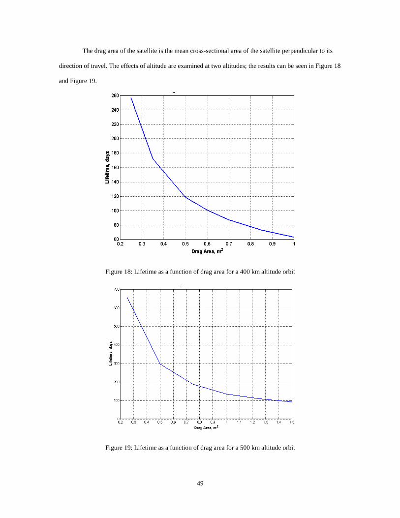
49
The drag area of the satellite is the mean cross-sectional area of the satellite perpendicular to its
direction of travel. The effects of altitude are examined at two altitudes; the results can be seen in Figure 18
and Figure 19.
Figure 18: Lifetime as a function of drag area for a 400 km altitude orbit
Figure 19: Lifetime as a function of drag area for a 500 km altitude orbit

50
Inclination of the orbit effects the coverage of a satellite. Inclination analysis is performed and
displayed in Figure 20.
Figure 20: Lifetime as a function of orbit inclination
For all calculations the decay altitude is 300 km. The decay altitude is the altitude at which the
satellite’s orbit is determined to be decayed. This is the altitude at which lifetime calculations stop.
3.2 Summary
Chapter three introduces the two main parameters in choosing an orbit for the VASCAT. A
method for predicting Earth ground coverage is presented which is useful in choosing an orbit or predicting
mission capabilities. Also, the variations of lifetime with orbit altitude, drag area, drag coefficient, and
inclination are presented in chapter three. These variations provide the minimum orbital parameters for the
VASCAT. The lifetime information can be combined with the coverage information to determine the
optimal orbit for the VASCAT.

51
Chapter 4: Cost Analysis
A cost model predicts the overall cost of a project, from initial research and testing to its final end-
of-life costs. Cost modeling is used as a method of maximizing performance while remaining within
budgetary constraints, rather than estimating the cost of a project with given performance parameters.20
The parametric cost estimation method (PECM) uses mathematical relationships to relate input
parameters directly to the cost of the project. The equations used are known as the cost estimation
relationships (CER) and are expressed as a function of the cost drivers. Several assumptions are made
when using a PECM. The most predominant assumption is that the PECM is based on historical spacecraft
mission costs. A specific PECM is limited on the type and size of spacecraft for which it is effective. 20
The PECM used for the VASCAT is similar to an example for scientific small LEO satellites
found in the Space Mission Analysis and Design reference. 20 The VASCAT fits into this description for
the PECM. Table 28 shows the output of the PECM using parameters from the VASCAT. The total cost
of producing the VASCAT is found by summing the values in the right hand column of Table 28. The cost
to produce the VASCAT is approximately $16 million to $49 million. This cost is greater than HokieSat's
budget of $1.5 million, which does not include testing costs or student labor costs.
NASA's Johnson Space Center provides the public with an online cost estimator for different types
of spacecraft. One of the spacecraft options is a scientific satellite with mass as the only input. The mass
of the VASCAT is assumed to be 40 kg. The NASA calculator outputs a development and production cost
of approximately $15 million and an operations cost of approximately $0.5 million per year.13
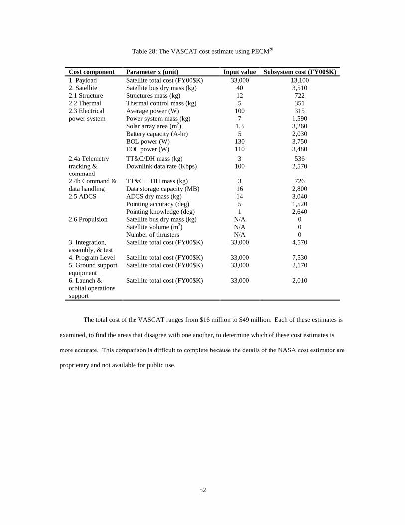
52
Table 28: The VASCAT cost estimate using PECM20
Cost component Parameter x (unit) Input value Subsystem cost (FY00$K) 1. Payload Satellite total cost (FY00$K) 33,000 13,100 2. Satellite Satellite bus dry mass (kg) 40 3,510
2.1 Structure Structures mass (kg) 12 722 2.2 Thermal Thermal control mass (kg) 5 351
Average power (W) 100 315
Power system mass (kg) 7 1,590
Solar array area (m2) 1.3 3,260
Battery capacity (A-hr) 5 2,030
BOL power (W) 130 3,750
2.3 Electrical power system
EOL power (W) 110 3,480
TT&C/DH mass (kg) 3 536 2.4a Telemetry tracking & command
Downlink data rate (Kbps) 100 2,570
TT&C + DH mass (kg) 3 726 2.4b Command & data handling Data storage capacity (MB) 16 2,800
ADCS dry mass (kg) 14 3,040
Pointing accuracy (deg) 5 1,520 2.5 ADCS
Pointing knowledge (deg) 1 2,640 Satellite bus dry mass (kg) N/A 0
Satellite volume (m3) N/A 0 2.6 Propulsion
Number of thrusters N/A 0
3. Integration, assembly, & test
Satellite total cost (FY00$K) 33,000 4,570
4. Program Level Satellite total cost (FY00$K) 33,000 7,530 5. Ground support equipment
Satellite total cost (FY00$K) 33,000 2,170
6. Launch & orbital operations support
Satellite total cost (FY00$K) 33,000 2,010
The total cost of the VASCAT ranges from $16 million to $49 million. Each of these estimates is
examined, to find the areas that disagree with one another, to determine which of these cost estimates is
more accurate. This comparison is difficult to complete because the details of the NASA cost estimator are
proprietary and not available for public use.

53
Chapter 5: Summary, Conclusions, and Remaining Work
The satellite design VASCAT detailed in this paper is a preliminary design incorporating the
µMAPS instrument into a host spacecraft. The VASCAT design, based on Virginia Tech’s existing
nanosatellite HokieSat, supports the µMAPS instrument with a minimum mission lifetime of one year.
The preliminary design of the required subsystems is described in this report. Component level
definitions are given for the ADCS, thermal, and power subsystems. The VASCAT is configured for body-
mounted solar cells and room to house the instrument and all other subsystem components. The structure
design incorporates the µMAPS instrument’s existing mounting feet. Preliminary structural analysis is
used to size the primary structure. The orbital analysis presented lays the groundwork for determining a
more definite orbit to adequately complete the mission. The satellite is designed to meet the desired
lifetime requirements of one year without propulsion. The addition of a digital camera is not discussed in
detail, but it has been considered by all subsystems and can fit into the VASCAT design.
The AMSAT frequency is proposed to allow high school students to participate in the VASCAT
mission. This frequency downloads data from both the µMAPS instrument and the proposed digital
camera. The camera takes pictures during data collection. The AMSAT downlink needs to be further
defined to accomplish the download of atmospheric pictures and the secondary educational requirements.
All subsystem designs are incomplete. Further knowledge of the AMSAT hardware is required to
fully define its use. The interior of the VASCAT, including component placement and wiring paths, must
be configured. A launch vehicle must be chosen for further structural analysis and design. Most
importantly, a design and fabrication budget is required to continue high level subsystem design.

54
References
1. Analytical Graphics, Inc. “Analytical Graphics, Inc.” 2002. <http://www.stk.com/> (24 March,
2002)
2. AMSAT. "AMSAT From A to Z." 2002. <http://www.amsat.org/amsat/a_to_z.html> (4 May,
2002)
3. C&R Technologies, Inc. "SINDA/FLUINT 4.4 manual." 2002.
<www.sindaworks.com/docs/manuals/sf44main.zip> (2 May, 2002)
4. Cengel, Y.A. Introduction to Thermodynamics and Heat Transfer. Irwin/Mcgraw-Hill. Botson,
Massachusetts. 1997.
5. Findlay, S. ION-F Flight Communications Design Specification. University of Washington,
Seattle, Washington. Issue date: 14 September, 2000. <http://www.aoe.vt.edu/~hokiesat>
6. Gilmore, D.G. and Bello, M. (editors). Satellite Thermal Control Handbook. The Aerospace
Corporation Press. El Segundo California. 1994.
7. Harvey, A.C. HokieSat Interface Control Document, Revision VT ICD C-2. Virginia Polytechnic
Institute and State University, Blacksburg, Virginia. Issue date: 2 November, 2000.
<http://www.aoe.vt.edu/~hokiesat>
8. HokieSat webpage, webmaster Jana L. Schwartz. Updated 14 March, 2002.
<http://www.aoe.vt.edu/~hokiesat>
9. Incropera, F.P. and DeWitt, D.P. Fundamentals of heat and mass transfer, fourth edition. School
of Mechanical Engineering, Purdue Univ. John Wiley and Sons. New York. 1996.
10. Isakowitz, S.J., Hopkins, J.P. and Hopkins, J.B. International Reference Guide to Space Launch
Systems: Third Edition. AIAA Publishing. Reston, Virginia. 1999.
11. Ithaco. “Ithaco Home Page.” 1997. <http://www.ithaco.com/> (28 April, 2002)
12. Jensen, J.D. and Swenson C.M. Command and Data Handling Subsystem Design for the
Ionospheric Observation Nanosatellite Formation. Utah State University, Logan, Utah. Issue date:
28 June, 2000. <http://www.aoe.vt.edu/~hokiesat>
13. Johnston Space Center. “JSC Homepage.” 2002. <http://www.jsc.nasa.gov/> (20 April, 2002)

55
14. Sanyo North America Corporation. “Nickel-Metal Hydride Battery HR-4/3 FAU 4500.” 2001.
<www.sanyo.com> (26 April, 2002)
15. Sarafin, T. Spacecraft Structures and Mechanisms from Concept to Launch.
Torrance: Microcosm Press. 1995.
16. Spectrolab. "Spectrolab Products." 2000. <http://www.spectrolab.com/prd/prd.htm> (21 March,
2002)
17. Systron Donner. “Systron Donner Inertial Division.” 1998. <http://www.systron.com/> (20 April,
2002)
18. Valley Forge Composite Technologies. “VFCF: Valley Forge Composite Technologies.” 2001.
<http://www.vfct.com/> (20 April, 2002)
19. Walberg, G., Reichle, H.G. and Morrow, W.H. Design and Testing of MicroMAPS Gas Filter
Correlation Radiometer. 21 January 1999.
20. Wertz, J.R. and Larson, W.J. (editors). Space Mission Analysis and Design 3rd Edition. Microcosm
Inc. El Segundo, California. 1999.

56
Appendix A: MATLAB Power Code
% This function takes the height and major diameter of a hexagonal prism % and returns the projected area of the eight faces. % This function returns a matrix eight by N (time step) with projected areas % for the faces in the rows % and the columns are different instances in the orbit. function pete = bidwell(height,diameter) W = 0*pi/180; inc = 50*pi/180; si = [1 0 0]'; a = 6778; mu = 3.986*10^14; Gs = 1358; sce = 0.20; Ld = 0.02; life = 1; Id = 0.88; n = sqrt(3.986*10^5 / a^3); Period = 2*pi/n; Npoints = 900; tspan = linspace(0,Period,Npoints); facesb = faces(height,diameter); R13 = R1(inc)*R3(W); Roop = [0 1 0; 0 0 -1; -1 0 0]; for ti = 1:1:Npoints % Calculation of True Anomaly u = n * (tspan(ti) - 0); % Rotations Roi = Roop*R3(u)*R13; Rbo = eye(3,3); %Orbital frame aligned with body frame Rbi = Rbo * Roi; sb = Rbi * si; rper = [a*cos(u) a*sin(u) 0]'; ri = Roi*rper; alpha = atan(6378/norm(ri)); %Eclipse angle if u <= alpha %If u is less than or equal to alpha, then the satellite is eclipsed eclipse=0; %eclipse=0 when satellite is eclipsed and eclipse=1 all other times. elseif u >= 2*pi-alpha eclipse=0; else eclipse=1; end for i = 1:8 costheta(i) = sb' * facesb(1:3,i); if costheta(i) <= 0 costheta(i) = 0; end Aproj(i,ti) = costheta(i) * facesb(4,i) * eclipse; %Projected Area end
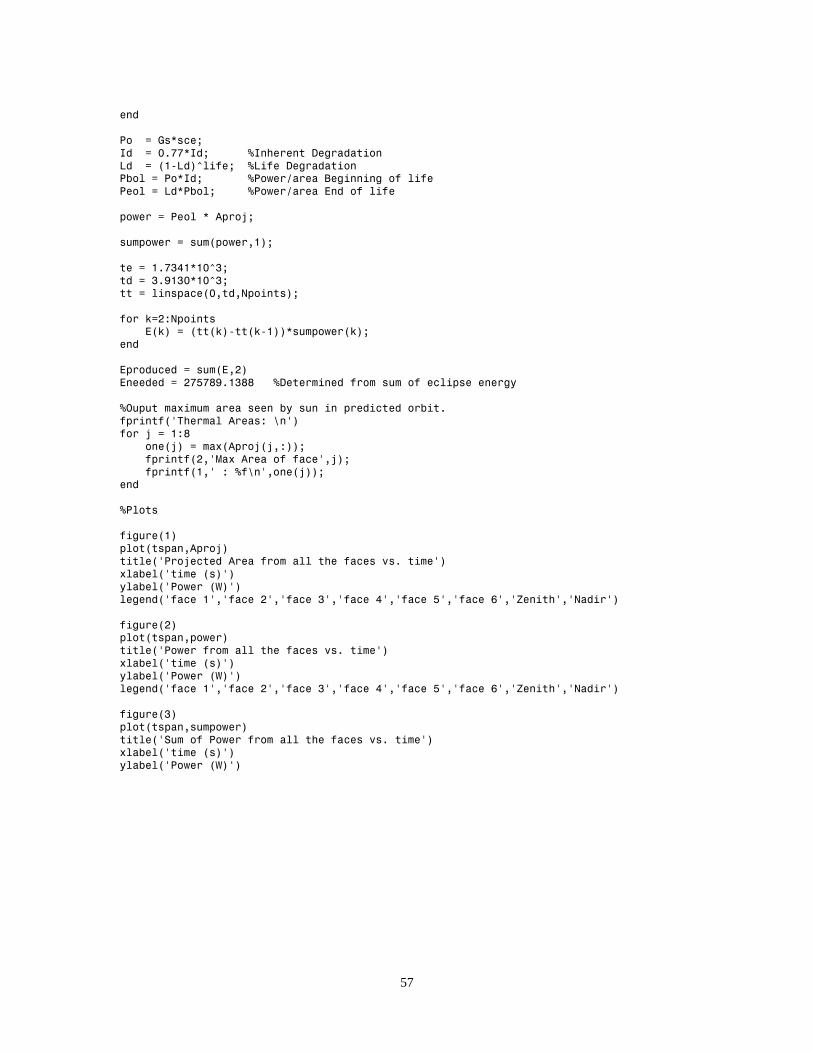
57
end Po = Gs*sce; Id = 0.77*Id; %Inherent Degradation Ld = (1-Ld)^life; %Life Degradation Pbol = Po*Id; %Power/area Beginning of life Peol = Ld*Pbol; %Power/area End of life power = Peol * Aproj; sumpower = sum(power,1); te = 1.7341*10^3; td = 3.9130*10^3; tt = linspace(0,td,Npoints); for k=2:Npoints E(k) = (tt(k)-tt(k-1))*sumpower(k); end Eproduced = sum(E,2) Eneeded = 275789.1388 %Determined from sum of eclipse energy %Ouput maximum area seen by sun in predicted orbit. fprintf('Thermal Areas: \n') for j = 1:8 one(j) = max(Aproj(j,:)); fprintf(2,'Max Area of face',j); fprintf(1,' : %f\n',one(j)); end %Plots figure(1) plot(tspan,Aproj) title('Projected Area from all the faces vs. time') xlabel('time (s)') ylabel('Power (W)') legend('face 1','face 2','face 3','face 4','face 5','face 6','Zenith','Nadir') figure(2) plot(tspan,power) title('Power from all the faces vs. time') xlabel('time (s)') ylabel('Power (W)') legend('face 1','face 2','face 3','face 4','face 5','face 6','Zenith','Nadir') figure(3) plot(tspan,sumpower) title('Sum of Power from all the faces vs. time') xlabel('time (s)') ylabel('Power (W)')

58
Appendix B: HokieSat Loop Antenna
Figure 21: Loop antenna assembly from HokieSat drawing package
Figure 22: Copper tube loop from HokieSat drawing package

59
Appendix C: MATLAB Earth Ground Coverage Code
% This code takes the orbital elements and propagates the orbit to determine the amount % of time a given point on Earth’s surface is in view % Input parameters mu=3.986004418*10^5; % Earth's gravitational constant (km^3/s^2) cf=pi/180; % conversion from degrees to radians Re=6378.13649; % radius of the Earth in nmi c=2.99792458*10^5; % speed of light (km/s) H=500; % satellite altitude (km) a=Re+H; % semi-major axis (km) e=0; % eccentricity i=57*cf; % inclination w=0*cf; % argument of perigee an=0*cf; % longitude of ascending node p=a*(1-e^2); h=sqrt(mu*p); % momentum (km^2/s) period=2*pi*sqrt(a^3/mu); % orbital period (s) n=sqrt(mu/(a^3)); % mean motion (rad/s) % calculate FOV rho=asin(Re/(Re+H))/cf; % angular radius of the earth nadir=1.5; % max off-nadir angle of instrument field of view elevation=acos(sin(nadir*cf)/sin(rho*cf))/cf; % cooresponding elevation angle FOV=90-elevation-nadir; % field of view of instrument on Earth's surface lat=0; q=1; COV=zeros(91,361); % **TARGETS** while lat<=90 %latitude of the target lon=0; s=1; while lon<=360 %longitude of the target if lat<0 phi=(90-lat)*cf; z=Re*cos(phi); elseif lat>=0 phi=(90-lat)*cf; z=Re*cos(phi); end theta=lon*cf; x=Re*sin(phi)*cos(theta); y=Re*sin(phi)*sin(theta); target=[x y z]; % target radius vector in ECF tmag=norm(target); % magnitude of target vector in ECF f=0; % true anomaly M=0; % mean anomaly j=1; while M<=100*2*pi t=M/n; o(j)=an+7.292123517*(10^-5)*t; % right ascension of ascending node

60
% angular velocity of Earth = 2* pi rad / 23.934444 hr = 7.292123517E-5 rad/s k=2; E(1)=100; % E=eccentric anomaly E(2)=200; if e==0 E=M; elseif M==0 E=0; else while ( ( (E(k-1)/E(k))<=0.999) | ( (E(k-1)/E(k) )>=1.001) ) E(k+1)=E(k)-((E(k)-M-e*sin(E(k)))/(1-e*cos(E(k)))); k=k+1; end E=E(end); end if E<=pi f=acos((e-cos(E))/(e*cos(E)-1)); else f=-acos((e-cos(E))/(e*cos(E)-1)); end % calculate radius and velocity in ECF rsca=p/(1+e*cos(f)); % scalar radius (perifocal) vr=sqrt(mu/p)*e*sin(f); % perpendicular velocity (perifocal) vt=h/(rsca); % tangential velocity (perifocal) % transformation matrix from perifocal to ECF Ar11=cos(o(j))*cos(w+f)-sin(o(j))*cos(i)*sin(w+f); Ar21=sin(o(j))*cos((w+f))+cos(o(j))*cos(i)*sin(w+f); Ar31=sin(i)*sin(w+f); Ar=[Ar11 Ar21 Ar31]; % transformation matrix from perifocal to ECF At11=-cos(o(j))*sin(w+f)-sin(o(j))*cos(i)*cos(w+f); At21=-sin(o(j))*sin(w+f)+cos(o(j))*cos(i)*cos(w+f); At31=sin(i)*cos(w+f); At=[At11 At21 At31]; rsat=rsca*Ar; % satellite radius vector in ECF smag=norm(rsat); % magnitude of satellite radius
vector in ECF (km) vsat=vr*Ar+vt*At; % velocity vector in ECF vmag=norm(vsat); % magnitude of velocity vector (km/s) % find whether the target is in view of the satellite ECA=(180/pi)*acos((dot(rsat, target)) / (smag*tmag)); % earth center angle
(degrees) % **RESULTS** if ECA>=FOV anamoly(j)=f; else R=target-rsat; % resultant vector (satellite to
target) Rmag=norm(R); % magnitude of the resultant vector anamoly(j)=f; % vector to store f values Mdeg=M*180/pi; COV(q,s)=COV(q,s)+1;
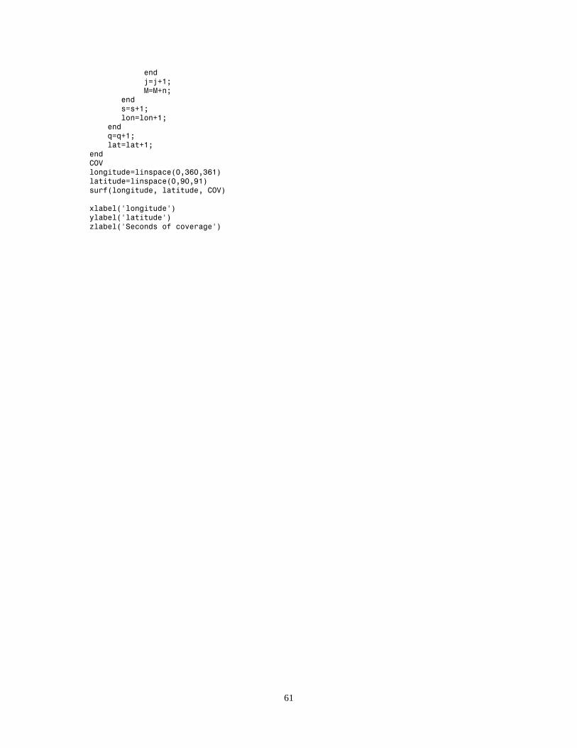
61
end j=j+1; M=M+n; end s=s+1; lon=lon+1; end q=q+1; lat=lat+1; end COV longitude=linspace(0,360,361) latitude=linspace(0,90,91) surf(longitude, latitude, COV) xlabel('longitude') ylabel('latitude') zlabel('Seconds of coverage')
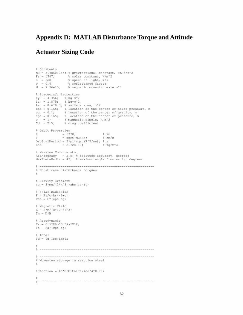
62
Appendix D: MATLAB Disturbance Torque and Attitude
Actuator Sizing Code
% Constants mu = 3.986012e5; % gravitational constant, km^3/s^2 Fs = 1367; % solar constant, W/m^2 c = 3e8; % speed of light, m/s q = 0.6; % reflectance factor M = 7.96e15; % magnetic moment, tesla-m^3 % Spacecraft Properties Iy = 4.356; % kg-m^2 Iz = 1.875; % kg-m^2 As = 0.6*0.3; % surface area, m^2 cps = 0.165; % location of the center of solar pressure, m cg = 0.1; % location of the center of gravity, m cpa = 0.165; % location of the center of pressure, m D = 1; % magnetic dipole, A-m^2 Cd = 2.5; % drag coefficient % Orbit Properties R = 6778; % km V = sqrt(mu/R); % km/s OrbitalPeriod = 2*pi*sqrt(R^3/mu); % s Rho = 2.72e-12; % kg/m^3 % Mission Constraints AttAccuracy = 2.5; % attitude accuracy, degrees MaxThetaNadir = 45; % maximum angle from nadir, degrees % ------------------------------------------------------------ % Worst case disturbance torques % % Gravity Gradient Tg = 3*mu/(2*R^3)*abs(Iz-Iy) % Solar Radiation F = Fs/c*As*(1+q); Tsp = F*(cps-cg) % Magnetic Field B = 2*M/(R*10^3)^3; Tm = D*B % Aerodynamic Fa = 0.5*Rho*Cd*As*V^2; Ta = Fa*(cpa-cg) % Total Td = Tg+Tsp+Tm+Ta % % ------------------------------------------------------------ % ------------------------------------------------------------ % Momentum storage in reaction wheel % hReaction = Td*OrbitalPeriod/4*0.707 % % ------------------------------------------------------------

63
% ------------------------------------------------------------ % Momentum storage in momentum wheel % hMomentum = Td*OrbitalPeriod/4/(AttAccuracy*pi/180) % % ------------------------------------------------------------