NUREG/CR-6918, Rev 4

VARSKIN+ 1.0

A Computer Code for Skin Contamination and Dosimetry Assessments

Office of Nuclear Regulatory Research

NUREG/CR-6918, REV 4

VARSKIN+ 1.0

A Computer Code for Skin Contamination and Dosimetry Assessments

Office of Nuclear Regulatory Research

Manuscript Completed: April 2021 Date Published: July 2021 Prepared by: D.M. Hamby C.D. Mangini J.M. Luitjens D.L. Boozer Z.G. Tucker C.T. Rose R.S. Flora Renaissance Code Development, LLC Corvallis, Oregon V. Shaffer, NRC Project Manager

iii

ABSTRACT

VARSKIN+ is a U.S. Nuclear Regulatory Commission (NRC) computer code used by staff members and NRC licensees to calculate occupational dose to the skin resulting from exposure to radiation emitted from hot particles or other contamination on or near the skin. These assessments are required by Title 10 of the Code of Federal Regulations (10 CFR) 20.1201(c), which states that the assigned shallow dose equivalent is to the part of the body receiving the highest exposure over a contiguous 10 cm2 of skin at a tissue depth of 0.007 centimeters (7 mg/cm2). Additionally, NRC staff evaluate radioactive intakes through wounds pursuant to 10 CFR 20.1202(d). VARSKIN+ can be used to perform wound dose assessments if the metabolic modeling and dosimetry methods are consistent with NRC regulations (e.g., use of 10 cm2 averaging area for skin dose assessments and tissue or organ weighting factors as defined in 10 CFR 20.1003). The VARSKIN+ computer code, an algorithm to calculate skin dose from radioactive skin contamination, has been modified on several occasions. As in previous versions, predefined source configurations are available in VARSKIN+ to allow simulations of point, disk, cylinder, sphere, slab, and syringe sources. Improvements to earlier versions included enhanced photon and electron dosimetry models, as well as models to account for airgap and cover materials. VARSKIN+ gives the user the option to have the code automatically include all decay products in dosimetry calculations or to allow the user to manually add progeny. Both ICRP 38, “Radionuclide Transformations – Energy and Intensity of Emissions” (1983), and ICRP 107, “Nuclear Decay Data for Dosimetry Calculations” (2008), nuclide libraries are available at the user’s option and contain data on gamma rays, X rays, beta particles, internal conversion electrons, and Auger electrons. Although the user can choose any dose-averaging area, the default area for skin dose calculations is 10 square centimeters, to conform to the requirements in 10 CFR 20.1201(c). A variety of unit options are provided (including both British and International System (SI) units), and the source strength can be entered in units of total activity or distributed in units of activity per unit volume. The photon model accounts for photon attenuation, charged particle buildup, and electron scatter at all depths in skin. The model allows for volumetric sources and clothing or airgaps between source and skin. The electron dosimetry model has a robust accounting for electron energy loss and particle scatter. Dose point kernels are Monte-Carlo based and results agree very well with Electron Gamma Shower (EGS) and Monte Carlo N Particle (MCNP) probabilistic simulations. With the release of VARSKIN+ three new physics modules are introduced: (1) wound dosimetry; (2) neutron dosimetry; and (3) eye dosimetry. Skin and wound dosimetry implement a new alpha dosimetry model for shallow skin assessments. The new VARSKIN+ user interface is written in Java with all scientific coding updated to Fortran 2018. A chronology of VARSKIN development since its inception in 1987 is provided below.

v

TABLE OF CONTENTS

ABSTRACT ............................................................................................................................. iii

LIST OF FIGURES........................................................................................................ vii

LIST OF TABLES .......................................................................................................... xi

ACKNOWLEDGMENTS .............................................................................................. xiii

ABBREVIATIONS AND ACRONYMS .......................................................................... xv

1 INTRODUCTION ......................................................................................................... 1

2 VARSKIN+ USER’s MANUAL ................................................................................... 3 2.1 Introduction to VARSKIN+ ............................................................................................... 3 2.2 Running SkinDose ........................................................................................................... 5

2.2.1 Source Geometry .............................................................................................. 5 2.2.2 Adding Radionuclides to the Exposure Scenario ............................................... 7 2.2.3 Geometry Parameters ..................................................................................... 10 2.2.4 Default State .................................................................................................... 11 2.2.5 Covers and Airgap ........................................................................................... 13 2.2.6 Special Options ............................................................................................... 15 2.2.7 Calculating Dose ............................................................................................. 16 2.2.8 Dosimetric Output ............................................................................................ 16

2.3 Running WoundDose .................................................................................................... 16 2.3.1 User Inputs ...................................................................................................... 17 2.3.2 Scenario Definition .......................................................................................... 18 2.3.3 Executing Dose Calculations ........................................................................... 18

2.4 Running NeutronDose ................................................................................................... 19 2.4.1 Source Selection ............................................................................................. 19 2.4.2 Defining the Dose Scenario ............................................................................. 20 2.4.3 Calculating Dose ............................................................................................. 21

2.5 Running EyeDose ......................................................................................................... 21 2.5.1 Dose Scenario ................................................................................................. 22 2.5.2 Running Calculations in EyeDose .................................................................... 23 2.5.3 Results ............................................................................................................ 23

2.6 Exiting VARSKIN+ ......................................................................................................... 24

3 SKIN DOSIMETRY MODEL ..................................................................................... 25 3.1 Electron Dosimetry ........................................................................................................ 25

3.1.1 Dose-Point Kernels .......................................................................................... 25 3.1.2 Numerical Integration of Dose-Point Kernels ................................................... 28 3.1.3 Nonhomogeneous Dose-Point Kernels ............................................................ 30 3.1.4 Backscatter Model ........................................................................................... 31 3.1.5 Scaling Models ................................................................................................ 37 3.1.6 Verification and Validation ............................................................................... 42 3.1.7 Limitations ....................................................................................................... 45

3.2 Photon Dosimetry .......................................................................................................... 46

vi

3.2.1 Off-Axis Scatter Correction .............................................................................. 49 3.2.2 Integration Methods ......................................................................................... 50 3.2.3 Attenuation Coefficients for Cover Materials .................................................... 52 3.2.4 Off-Axis Calculation of Dose ............................................................................ 52 3.2.5 Verification and Validation ............................................................................... 56 3.2.6 Limitations ....................................................................................................... 58

3.3 Alpha Dosimetry ............................................................................................................ 58 3.4 Cover Layer and Airgap Models .................................................................................... 61 3.5 Volume-Averaging Dose Model ..................................................................................... 63

4 WOUND DOSIMETRY MODEL ................................................................................ 65 4.1 Intact Skin, Abrasions and Nonsevere Burns ................................................................. 65 4.2 Severe Burns, Lacerations and Penetrating Wounds ..................................................... 66 4.3 Shallow Dosimetry ......................................................................................................... 66 4.4 Local Dosimetry ............................................................................................................. 67 4.5 Systemic Dosimetry ....................................................................................................... 68

5 NEUTRON DOSIMETRY MODEL ............................................................................ 71 5.1 Neutron Source Term .................................................................................................... 71 5.2 Neutron KERMA ............................................................................................................ 73 5.3 Fractional Charged Particle Equilibrium fcpe ................................................................... 74 5.4 Evaluation of fcpe Verification/Validation ......................................................................... 76 5.5 Evaluation of KERMA .................................................................................................... 77 5.6 Neutron Dose from Radiative Capture ........................................................................... 82

6 EYE DOSIMETRY MODEL ....................................................................................... 85 6.1 Photon Dosimetry .......................................................................................................... 85 6.2 Electron Dosimetry ........................................................................................................ 92 6.3 Continuous Radiation Sources ...................................................................................... 99 6.4 Verification and Validation ........................................................................................... 100 6.5 Limitations (Off-Axis Sensitivity Analysis) .................................................................... 111

7 REFERENCES ....................................................................................................... 115

APPENDIX A EXAMPLES AND SOLUTIONS USING VARSKIN+ ............................. 1

vii

LIST OF FIGURES

Figure 1-1 Depiction of Cylindrical Dose-Averaging Volume ................................................. 1

Figure 2-1 SkinDose User Interface ...................................................................................... 5

Figure 2-2 Schematic Representations of the Six Geometry Options .................................... 6

Figure 2-3 Nuclide Selection Window .................................................................................... 9 Figure 2-4 Nuclide Information Window .............................................................................. 10 Figure 2-5 Slab Source Geometry Parameters (upper left) ................................................. 11

Figure 2-6 Schematic Showing the Cover Material and Air Gap Models ............................. 13

Figure 2-7 Multiple Cover Calculator Window ..................................................................... 14

Figure 2-8 Schematic Diagram of the Volume-Averaged Dose Model Geometry ................ 15

Figure 2-9 The WoundDose User Interface ......................................................................... 16

Figure 2-10 The NeutronDose User Interface ....................................................................... 20

Figure 2-11 “Source Type” Window....................................................................................... 21

Figure 2-12 The EyeDose User Interface .............................................................................. 22

Figure 2-13 EyeDose “Nuclide Source” Window with User Input Fields ................................ 24

Figure 3-1 Schematic of EGSnrc Geometry for Determining Point-Source Radial DPKs ................................................................................................................. 27

Figure 3-2 Scaled Absorbed Dose Distributions for 0.1 MeV Electrons in an Infinite Homogeneous Water Medium............................................................................ 28

Figure 3-3 Scaled Absorbed Dose Distributions for 1.0 MeV Electrons in an Infinite Homogeneous Water Medium............................................................................ 28

Figure 3-4 Schematic Representation of the Eight-Panel Quadrature Routine Used to Calculate Dose for a Symmetric Source (redrawn from Durham 2006) .......... 30

Figure 3-5 Schematic Demonstrating Conditions in Which Full Source/Water Scattering Corrections are Applied ..................................................................... 33

Figure 3-6 Schematic Demonstrating Conditions in Which Partial Source/Water Scattering Corrections are Applied ..................................................................... 34

Figure 3-7 Schematic Illustrating Electron Energy Limitations of Side-Scatter Corrections ........................................................................................................ 35

Figure 3-8 Schematic iIllustrating Parameters Used to Determine the Amount of Side-Scatter Correction Applied to High-Energy Electrons Emitted from Large Sources ................................................................................................... 36

Figure 3-9 Schematic Demonstrating Conditions in Which a Full Air/Water Scattering Corrections are Applied...................................................................................... 37

Figure 3-10 Schematic Demonstrating Conditions in Which Air/Water Scattering Corrections are Applied...................................................................................... 37

viii

Figure 3-11 Comparison of 1 MeV Electron DPKs for the Homogeneous Water Case and the Case When the Electron Traverses an Iron Source of Thickness 0.022 cm ............................................................................................................ 38

Figure 3-12 Example of Depth Scaling on the Homogeneous DPK Curve ............................ 39

Figure 3-13 3D Plot of Depth-Scaling Data for All Source Materials Modeled ....................... 40

Figure 3-14 Example of Energy Scaling on the Homogeneous DPK Curve Presented in Figure 3-13 ..................................................................................................... 41

Figure 3-15 3D Plot of Energy-Scaling Data for All Source Materials Modeled ...................... 42

Figure 3-16 Depiction of Methods for Determining Integration Segments of the Dose-Averaging Disk ................................................................................................... 50

Figure 3-17 Relative Dose as a Function of the Number of Segments in a Numerical Integration (Iterations), by Method ..................................................................... 51

Figure 3-18 Dose-Averaging Disk with the Source Point Located on Axis ............................. 53

Figure 3-19 Dose-Averaging Disk Located at Depth h Beneath an Offset Point Source ........ 53

Figure 3-20 Dose-Averaging Disk with the Source Point Located Off Axis, Yet Still Over the Averaging Disk .................................................................................... 54

Figure 3-21 Relationship Between the Source-Averaging Disk and One of the Radii for Dose Calculation ........................................................................................... 54

Figure 3-22 Dose-Averaging Disk from Above with the Source Point Located Off Axis, Far Enough Removed to be Off the Averaging Disk ........................................... 55

Figure 3-23 Diagram of Alpha Source Over the Skin Surface with Cover Materials of Cotton, Latex, and Air ........................................................................................ 59

Figure 3-24 Schematic of a Generic Dose Calculation Performed by SkinDose for the Cylinder Geometry ............................................................................................. 62

Figure 4-1 General Compartment Model of the Biokinetics of Radionuclides and/or Radioactive Materials Deposited in a Wound (taken from NCRP 156) ............... 68

Figure 5-1 PSTAR versus Evaluated Data .......................................................................... 76

Figure 5-2 fcpe Comparisons (a) 5 MeV (b) 10 MeV (c) 14 MeV (d) 20 MeV ........................ 77

Figure 5-3 (a) Neutron KERMA Versus Energy and Contribution per Element Compared with ICRU 63. (b) Neutron KERMA Versus Energy Detailed at the Higher Incident Neutron Energies, Again Compared to ICRU 63 and to Liu and Chen (2008) ...................................................................................... 78

Figure 5-4 Threshold Reactions in Each of the Four Constituents Accounted for in KERMA as a Function of Incident Neutron Energy ............................................. 79

Figure 5-5 Percent Difference Between Neutron Dose Using ENDF Files versus ICRU 63 ............................................................................................................. 80

Figure 5-6 Reaction-Dependent KERMA in the Thermal Energy Range ............................. 80

Figure 5-7 Reaction-Dependent KERMA in the Intermediate Energy Range ....................... 81

Figure 5-8 Reaction-Dependent KERMA in the Fast Energy Range.................................... 82

ix

Figure 5-9 ICRP 23 Absorbed Fraction of Photon Energy Emitted from the Body and Absorbed in the Body ......................................................................................... 83

Figure 5-10 Absorbed Dose Due to Neutrons and Photons as a Function of Incident Neutron Energy .................................................................................................. 84

Figure 6-1 Eye Geometry Illustrating the Important Parameters Used in the Deterministic Dosimetry Model ........................................................................... 85

Figure 6-2 Photon Dosimetry Shaping Parameters Plotted as a Function of Energy ........... 87

Figure 6-3 Illustration of the Mathematical Parameters of the Shielded Model .................... 89

Figure 6-4 Shielded Dose Plotted as a Function of Unshielded Dose .................................. 90

Figure 6-5 Mass Attenuation Coefficient for Lead ................................................................ 91

Figure 6-6 The Switching Functions B+(q,s) and B-(q,s) with q = 1 and s = 5 ....................... 93

Figure 6-7 Total Dose to the Lens from 0.65 MeV Electrons with the Bremsstrahlung KERMA Called Out ............................................................................................ 93

Figure 6-8 Total Dose to the Lens from 0.65 MeV Electrons on Log-Log Axes ................... 94

Figure 6-9 Schematic Representation of How Curved Surfaces Result in Dose from Scattered Electrons ............................................................................................ 95

Figure 6-10 Lens Dose from 1 MeV Electrons on both Linear-Log and Log-Log Axes .......... 96

Figure 6-11 Lens Dose from 3 MeV Electrons on both Linear-Log and Log-Log Axes .......... 97

Figure 6-12 Comparison of the Dose for 0.65 MeV Electron Point Sources in Air and in Vacuum .......................................................................................................... 98

Figure 6-13 Component Breakdown of the Electron Dosimetry Model .................................. 99

Figure 6-14 An Empirical Function Fitted Against the Absorbed Dose to the Lens for 1 MeV Photons in Air .......................................................................................... 101

Figure 6-15 A Weighted MPE Residual Plot for the Photon Dosimetry Model Empirical Fit. The Weighting Used in this Fit Favored Smaller r Due to the Increased Certainty at those Distances ............................................................ 101

Figure 6-16 The Comparison Plot for a 1 MeV Photon Point Source. The Red Dashed Line Represents a Perfect Fit ........................................................................... 102

Figure 6-17 An Empirical Function Fitted Against the Mass Attenuation Coefficient for Photons in Air .................................................................................................. 102

Figure 6-18 The MPE Residual Plot for the Empirical Fit of the Mass Attenuation Coefficient in Air ............................................................................................... 103

Figure 6-19 Comparison Plot of Photon Model and 2,713 Data Points ................................ 103

Figure 6-20 The MPE of the Photon Dosimetry Model Plotted Against Photon Energy ....... 104

Figure 6-21 The MPE of the Photon Dosimetry Model Plotted Against Distance ................. 105

Figure 6-22 Plot of the MPE versus Energy for the Shielded Dose Model ........................... 105

Figure 6-23 Plot of the MPE versus Distance for the Shielded Dose Model ........................ 106

Figure 6-24 Comparison Plot for the Shielded Dose Model ................................................. 106

x

Figure 6-25 Comparison Plot for Unshielded Electrons in Air on Linear Axes ..................... 107

Figure 6-26 Comparison Plot for Unshielded Electrons in Air on Log-Log Axes .................. 107

Figure 6-27 Comparison Plot on Linear Axes for Electrons Shielded with Protective Leaded Eyewear .............................................................................................. 108

Figure 6-28 Comparison Plot on Log-Log Axes for Electrons Shielded with Protective Leaded Eyewear .............................................................................................. 108

Figure 6-29 Plot of the Lens Dose Rate for Selected Continuous Radiation Point Sources ........................................................................................................... 109

Figure 6-30 Schematic used by SkinDose to Simulate the Lens ......................................... 109

Figure 6-31 Comparison of Calculations Between SkinDose and this Model ....................... 110

Figure 6-32 Parameter Definitions for an Off-Axis Source ................................................... 111

Figure 6-33 D(r,θ) for Photons with r = 0.1, 1 and 10 cm and θ Ranging from 0° to 90° in 10° iIncrements ............................................................................................ 112

Figure 6-34 D(r,θ) for Electrons with r = 0.1, 1 and 10 cm and θ Ranging from 0° to 90° in 10° Increments ....................................................................................... 113

xi

LIST OF TABLES

Table 2-1 Default Values and Units for Geometry Parameters ........................................... 12 Table 2-2 Suggested Values for Cover Thickness and Density .......................................... 14

Table 3-1 List of Nuclides Used in Scaling and Scattering Models ..................................... 31 Table 3-2 Source Materials Used for Nonhomogeneous Electron DPK Testing ................. 31 Table 3-3 Comparison of Electron Shallow Dose Estimates using VARSKIN 3.1, 4,

5.3, 6.0, and V+ 1.0 SkinDose for a 37-kBq Point Source of Co-60 on the Skin for 1 hr ....................................................................................................... 43

Table 3-4 Comparison of Electron Shallow Dose Calculations from VARSKIN 3.1, 4, 5.3, 6.0, and V+ 1.0 SkinDose for Various Cover Material Configurations .......... 43

Table 3-5 Comparison of VARSKIN 4, 5.3, 6.0, and V+ 1.0 SkinDose of the Electron Dose (mGy) for a 1-hr Exposure to an Infinite Plane Source on the Skin ........... 44

Table 3-6 Dose (mGy) versus Depth for a 37 kBq/cm2 Distributed Disk Source of Y-90 and a 1-hr Exposure Time (Dose Averaged over 1 cm2) ............................... 44

Table 3-7 Function Coefficients ......................................................................................... 48 Table 3-8 Coefficients for Eq. [3.35] and [3.36] .................................................................. 52 Table 3-9 Comparison of Photon Shallow Dose Estimates using VARSKIN 3.1, 4,

5.3, 6.0, and V+ 1.0 SkinDose for a 37-kBq Point Source of Co-60 on the Skin for 1 hr ....................................................................................................... 56

Table 3-10 Comparison of Photon Shallow Dose Calculations from VARSKIN 3.1, 4, 5.3, 6.0, and V+ 1.0 SkinDose for Various Cover Material Configurations .......... 57

Table 3-11 Material Constants ............................................................................................. 59 Table 3-12 Coefficients for Equations .................................................................................. 60

Table 5-1 χ(E) Data for Nuclides which Spontaneously Fission (ICRP 107) ....................... 72 Table 5-2 χ(E) Data for Neutron-Induced Fission (Shultis & Faw 2000)............................. 72 Table 5-3 Characteristics of Alpha Reaction Sources Provided in V+ (Lorch 1973) ........... 73 Table 5-4 Characteristics of Photoneutron Sources Provided in V+ (Shutis and

Faw 2000) .......................................................................................................... 73 Table 5-5 ICRU Composition of Soft Tissue ....................................................................... 74 Table 5-6 Coefficients for Eqs. [5.6], [5.7], and [5.8] .......................................................... 75 Table 5-7 Coefficients for Eqs. [5.10] through [5.13] .......................................................... 76

Table 6-1 Coefficients for the Mass Attenuation Coefficient for Photons in Air Empirical Formula ............................................................................................................ 86

Table 6-2 Coefficients for the Shaping Parameters in the Photon Dosimetry Model .......... 88 Table 6-3 Coefficients for the Shaping Parameters of the Shielded Dose Equation ........... 92

xiii

ACKNOWLEDGMENTS

This report documents the work performed by Renaissance Code Development, LLC (RCD) for the U.S Nuclear Regulatory Commission (NRC) under Contract No. 31310018C0026. Staff at the Pacific Northwest National Laboratory authored initial versions of VARSKIN (US NRC 1987), with later versions amended at Colorado State University (US NRC 1992), the Center for Nuclear Waste Regulatory Analyses (US NRC 2006), and Oregon State University (US NRC 2011; US NRC 2014; US NRC 2018). RCD performed the activities described in this report on behalf of the NRC Office of Nuclear Regulatory Research, Division of System Analysis. This report is a product of RCD and does not necessarily reflect the views or regulatory position of the NRC. The authors are indebted to V. Shaffer, S. Bush-Goddard, J. Tomon, M. Saba, and S. Sherbini for their long-lasting support during development and maintenance of many of the dosimetry models now appearing in VARSKIN+. The team at RCD is very appreciative of the technical assistance received over the years from the following individuals: L. Anspach, J. Caffrey, G. Chabot, M. Charles, J. Chase, R. Clement, K. Consoni, J. DeCicco, E. Dickson, A. Di Pasqua, J. Dubeau, J. Dwyer, G. Edwards, E. Hanson, L. Howard, M. Jimenez, L. Johnston, M. Lantz, J. Lebda, H. Karagiannis, K. Krobl, P. Lee, S. Marshall, N. McDaniel, E. Mercer, D. Neville, R. Nimitz, B. Orr, J. Parson, B. Plain, S. Reese, A. Roecklein, M. Ryan, A. Salame-Alfie, K. Sejkora, L. Selvey, M. Stabin, R. Struckmeyer, G. Sturchio, M. Tang, B. Tharakan, M. Thornhill, D. Turner, T. Vandermey, and M. Wierzbicki.

xv

ABBREVIATIONS AND ACRONYMS

2D two-dimensional 3D three-dimensional BSCF backscatter correction factor CEDE committed effective dose equivalent CFR Code of Federal Regulations CPE charged particle equilibrium CSDA continuous slowing down approximation DDE deep dose equivalent DPK dose-point kernel DSP depth-scaling parameter EDK energy deposition kernel EGS electron gamma shower ENDF Evaluated Nuclear Data File EPRI Electric Power Research Institute ESP energy-scaling parameter ICRP International Commission on Radiological Protection ICRU International Commission on Radiation Units and Measurements KERMA kinetic energy released in matter LANL Los Alamos National Laboratory MCNP Monte Carlo N-Particle MPE mean percent error NCRP National Council on Radiation Protection and Measurement NIST National Institute of Standards and Technology NRC Nuclear Regulatory Commission RCD Renaissance Code Development, LLC RSO radiation safety officer SADD Scaled Absorbed Dose Distribution SDE shallow dose equivalent TCPE transient charged particle equilibrium V+ VARSKIN+

1

1 INTRODUCTION

The original VARSKIN computer code (US NRC 1987) was intended as a tool for the calculation of tissue dose at user-defined depths as the result of skin contamination. The contamination was assumed to be a point, or an infinitely thin disk source located directly on the skin. Soon after the release of VARSKIN, the industry encountered a “new” type of skin contaminant consisting of discrete microscopic radioactive fragments, called “hot particles”. These particles differ radically from uniform skin contamination in that they have a volume associated with them, and many of the skin exposures result from particles on the outside of protective clothing. These assessments are required by Title 10 of the Code of Federal Regulations (10 CFR) 20.1201(c), which states that the assigned shallow dose equivalent (SDE) is to the part of the body receiving the highest exposure over a contiguous 10 cm2 of skin at a tissue depth of 0.007 centimeters (7 mg/cm2). VARSKIN MOD2 (US NRC 1992) contained all the features of the original VARSKIN, with many significant additions. Features in MOD2 included the modeling of three-dimensional (3D) sources (cylinders, spheres, and slabs) that accounted for self-shielding, and modeling of materials placed between the source and skin (i.e., airgaps and covers) that could absorb electron energy and attenuate photons. VARSKIN MOD2 also used a correction for backscatter for one-dimensional and two-dimensional (2D) electron sources under limited conditions. Finally, the VARSKIN MOD2 package incorporated a user interface that greatly simplified data entry for calculating skin dose. MOD2 contained a volume-averaged dose model that has been retained in subsequent VARSKIN coding. The volume-averaging model allows the user to calculate dose averaged over a volume of tissue defined by a cylinder with a diameter equal to that of the dose-averaging area and bounded at the top and bottom by two user-selected skin depths (see Figure 1-1). This model is useful for calculations of dose that can be compared to the dose measured by a finite-volume instrument (e.g., a thermoluminescent dosimeter).

Figure 1-1 Depiction of Cylindrical Dose Averaging Volume (US NRC 1987)

2

Finally, VARSKIN MOD2 gave the user the ability to select a composite source term, thus allowing the calculation of total dose from a mixture of radionuclides instead of requiring the code to be executed separately for each constituent. This feature was upgraded in VARSKIN 3 (US NRC 2006), allowing the user to select up to twenty radionuclides in a single calculation. One drawback of removing this feature in VARSKIN 3 was that the user was forced to explicitly add radioactive progeny. Subsequent VARSKIN versions incorporate radioactivity progeny at the user’s discretion. Enhancements to VARSKIN 4 (US NRC 2011) focused on the photon dosimetry model. The photon model includes charged-particle buildup and subsequent transient equilibrium, along with photon attenuation, air and cover attenuation, and the option to model volumetric sources. The VARSKIN 5 (US NRC 2014) package updated electron dosimetry model to better account for charged-particle energy loss as the particle moves through the source, cover material, air, and tissue. VARSKIN 6 (US NRC 2018) further enhanced the physics models and the user interface. SkinDose, introduced in VARSKIN+, employs a new user interface written in Java and updated Fortran for physics calculations based on Fortran 2018 fundamentals. Speed increases of 25x have been realized in various data-handling routines of the updated Fortran. Chapter 2 of this report comprises the VARSKIN+ User’s Manual. It is subdivided into four segments and mimics the layout of the GUI. The segments are SkinDose, WoundDose, NeutronDose, and EyeDose. Chapter 3 discusses the technical basis for the SkinDose (classic VARSKIN) module, while Chapters 4, 5, and 6 describe the physics models employed for wound, neutron, and eye dosimetry. Verification and validation results for each of the four dosimetry modules are contained in the specific chapter describing the module. Appendix A provides a few sample problems for each dose module and the user is encouraged to become familiar with dosimetry functions by exercising each sample problem.

3

2 VARSKIN+ USER’S MANUAL

This section serves as the user’s guide for VARSKIN+ (V+). It includes operating instructions and a description of its features. Chapters 3 through 6 describe the computational dosimetry models for each of the four physics modules. 2.1 Introduction to VARSKIN+

VARSKIN was originally designed as a versatile calculational tool intended for use as an estimator of skin dosimetry from radioactive contamination and hot particles. In the 35 years since its introduction, the tool has grown into what is known as VARSKIN+, which includes the classic VARSKIN dosimetry module (SkinDose), a wound dosimetry module (WoundDose), a neutron dosimetry module (NeutronDose), and an eye dosimetry module (EyeDose). SkinDose calculates dose equivalent from photon, electron, and alpha radiation from more than 1,200 radionuclides that may be encountered in a variety of skin-contamination applications from laboratory use to medical and therapeutic applications. SkinDose can calculate the dose to averaging areas from a minimum of 0.01 cm2 to a maximum of 100 cm2, and airgaps between source and skin of up to 20 cm. SkinDose calculates shallow dose to an infinitely thin disk at a depth of 0.007 mg/cm2 in tissue for comparison to the NRC shallow dose limit of 0.5 gray (Gy) for both point and distributed sources. Other user-specified depths from zero to 2 cm are allowable. Users are cautioned that SkinDose is designed to calculate the dose to skin from skin contamination or sources close to the skin surface (within 20 cm). Using SkinDose to perform calculations that are beyond its intended application may result in erroneous dose estimates. SkinDose offers the option of dose calculations based on the decay data of International Commission on Radiological Protection (ICRP) 38, “Radionuclide Transformations – Energy and Intensity of Emission” (ICRP 1983), or ICRP 107, “Nuclear Decay Data for Dosimetric Calculations” (ICRP 2008). WoundDose is based on National Council on Radiological Protection and Measurement (NCRP) Report 156, “Development of a Biokinetic Model for Radionuclide-Contaminated Wounds and Procedures for Their Assessment, Dosimetry and Treatment” (NCRP 2007) and calculates shallow dose equivalent (SDE), local dose equivalent, and committed effective (and organ) dose equivalent from industrial or medical events resulting in the subdermal introduction of radioactivity following skin injury. The user will notice that many of the features of WoundDose are derived from the SkinDose module and their utilization is similar. Point-source and line-source geometries are allowable. NeutronDose estimates shallow tissue dose at a user-specified depth following exposure to a source of neutrons with energies ranging several orders of magnitude from thermal to fast. The user can select monoenergetic neutrons or can choose from a list of ICRP 107 nuclides and reaction compounds resulting in various neutron spectra. Neutrons are assumed to be orthogonally incident on the body. EyeDose allows for the evaluation of photon and electron dose to the lens of the human eye for radionuclides in the ICRP 38 or ICRP 107 database or for monoenergetic beams. The source of photons and electrons is assumed to be on-axis with the eyeball (i.e., the exposed individual is staring at the source). Lens dose is calculated for unshielded and shielded eyes. Shielding is provided by standard safety glasses containing 2 mm leaded glass.

4

To download VARSKIN+, locate the VARSKINPlus executable file (.exe) and place it on your desktop. Other than to clean up files and save memory, there is no need to uninstall previous versions of V+. New versions are installed in the same manner and multiple versions can be run simultaneously. The V+ app requires approximately 215 megabytes of disk space. If any of the V+ interface windows are not fully visible on the display screen, the user should adjust resolution and magnification as appropriate. Double-click the executable file to install V+. Once the installation is complete, you will see a shortcut for V+ on your desktop. To run V+, double-click the V+ icon. The initial user interface shown below is the first to appear; this interface acts as the central control panel and allows the user to select any of the four dosimetry modules (described below).

For the general user, access to V+ files is not required (and not recommended!). If such access is paramount, the V+ folder location can be found in the “Shortcut” tab of the Properties window (right click on the V+ shortcut icon and select “Properties”). The “Target” field contains the location on the user’s local machine where all files are stored. If a module locks up or otherwise malfunctions, there is the Reset Window option under the File dropdown that will restore its functionality. Reset Window can be used as well to clear and reset the inputs at any time.

5

2.2 Running SkinDose

To run SkinDose (classic VARSKIN), the user selects the SkinDose module from the initial V+ window. After selecting the SkinDose button, the user will see the interface window below (Figure 2-1). The user defines the exposure scenario by selecting and providing data entry fields in the input window. The inputs for SkinDose are defined in this section.

Figure 2-1 SkinDose User Interface. 2.2.1 Source Geometry

Although SkinDose allows the user to enter data in any order, it is best practice to input the source geometry first, because changing the geometry option will cause certain parameters to appear and others to be removed. Six geometry packages are available: point source, disk source (infinitely thin), cylinder source (thick), spherical source, slab source (rectangular), and syringe source. Source activity is assumed to be evenly distributed throughout the area or volume for all source geometries. The point source geometry (Figure 2-2(A)) is often used as an initial screening tool for contamination that is confined to an extremely small area of the skin, or for a conservative calculation to determine whether a regulatory limit is being approached or exceeded. The point source geometry does allow for self-shielding, so a 3D source geometry is best for particulate contamination. The point source model does not require any data describing the physical dimensions of the source and will generally yield the highest dose rate for a given activity of any of the available source geometries. For electron dosimetry, a point source is automatically modeled (due to historical code constraints) as a cylindrical source with a thickness of 1 micron, a radius of 1 micron, and a density of 0.001 grams per cubic centimeter (g/cm3).

6

Figure 2-2 Schematic Representations of the Six Geometry Options The infinitely thin disk source geometry model (Figure 2-2(B)) is simple and is recommended for modeling skin contamination events caused by liquid sources. The disk source geometry requires the user to enter either the source diameter or the source area at the bottom of the Disk Source Irradiation Geometry box. Entering the area of the contamination is useful for modeling sources when the area is known. Enter the area of the source in the textbox labeled “Source Area.” When the user enters the diameter of the source area, SkinDose calculates the area of the 2D disk with that diameter. Similarly, when the user enters the area of the source, SkinDose calculates the diameter of the disk with the same area. If the area of contamination is not circular, entering the area of the actual contamination will generally result in a reasonable estimation of skin dose. The cylindrical source model (Figure 2-2(C)) requires knowledge of density and two dimensions, the cylinder diameter and its height (thickness). The cylindrical source geometry assumes that the source is surrounded by air and that the entire bottom of the cylinder is in contact with skin or cover material. Of the two dimensions describing a cylinder, the calculated dose is much more sensitive to changes in the cylinder height as opposed to the cylinder diameter (US NRC 1992). The slab source geometry (Figure 2-2(D)) requires knowledge of density and three physical dimensions: the first side length, the second side length, and the slab’s thickness. Generally, as in the cylindrical model, slab thickness will have more influence on tissue dose than will lateral dimensions. The spherical source geometry (Figure 2-2(E)) is perhaps the simplest 3D geometry to use for dose calculations because it requires knowledge of source density and only one source dimension, its diameter. The spherical source geometry assumes that the source is surrounded by air and touches the skin or cover material only at the bottom point of the sphere. For photon dosimetry, it is assumed that the source material is equivalent to air for attenuation calculations. Choosing a spherical source will generally overestimate dose compared to a similarly sized

7

cylindrical source (same radius and length) with the same total activity. The air surrounding the bottom hemisphere does not shield the source particles as efficiently as the source material (which would be encountered by the particle in the cylinder or slab models), and a larger area of skin will be exposed, resulting in consistently higher doses. The syringe geometry (Figure 2-2(F)) has been reinstated in the SkinDose module. The user enters the length and diameter of the radioactivity fluid; the dimensions are those of the fluid and not the physical syringe. The syringe model essentially behaves like the cylinder model except that the cylinder would be standing on the skin surface and the syringe is lying on the skin surface. The following general rules should govern the choice of geometry package, progressing from the most conservative to least conservative dose estimate:

• If nothing is known about the particle size and shape, use the point source geometry option. This option is also recommended for a conservative approach for regulatory limits since the point geometry typically overestimates actual skin dose.

• If the diameter is known, but the thickness cannot be estimated, or if a distributed

source is being modeled (i.e., with a known source strength per unit area), use the two-dimensional disk source geometry option. If an infinite plane source is desired, a source area of at least 15 cm2 is generally sufficient.

• If the particle is known to be spherical (few particles are truly spherical), use the

spherical source geometry option.

• If the thickness and the diameter of the source can be estimated, but the shape is unknown, use the cylindrical source geometry option because this geometry requires only two dimensions (thickness and diameter) to describe the particle.

• If the particle is known to be rectangular, use the slab or cylinder source

geometry options. The height of the particle should be preserved, and the area of the contact surface should be selected such that the source volume is preserved. Executing both slab and cylinder will aid in providing bounding doses.

It is not intended that SkinDose models be used to simulate large volumetric sources and the user is cautioned against using dimensions greater than a few centimeters. For all source geometries, dose is averaged over an infinitely thin disk centered below the central axis of the source. 2.2.2 Adding Radionuclides to the Exposure Scenario

SkinDose employs two master decay libraries and a user library that contains only those radionuclides that have been selected and added by the user. Nuclide decay information is obtained from abridged datasets published by the ICRP, namely the ICRP 38 (1983) or ICRP 107 (2008) databases; SkinDose defaults to the ICRP 38 database. The user selects the nuclear database from which to extract decay data when radionuclides are selected from the master library to be added to the user library. Additionally, the user will choose between the

8

automatic inclusion of decay progeny (designated by “D”), or manual (or none) progeny selection. In addition to selecting the master library (either ICRP 38 or ICRP 107, with or without progeny), and the nuclide from that library, the user must specify an effective atomic number (Zeff) to characterize the source material in which the radioactivity is incorporated. The default value for Zeff is 7.42 (the effective atomic number of water), meaning the radioactivity itself is assumed to be dissolved or suspended in water. When the user chooses to include decay products (“D”), radioactive progeny follows the parent in secular equilibrium when selected from the master library. Selecting the non-progeny datasets will include only parent nuclides. The selection of decay progeny results in a single calculation of dose for the parent and progeny incorporating the entire decay chain (with branching ratios greater than 1 percent). Individual doses for each member of the chain are not provided. If this information is desired, the user may select the dataset(s) without progeny inclusion and manually select each member of the decay series. If evaluating dose from progeny alone, the user must note its half-life and include the correct dose calculation (decay corrected or not) in the dose estimate. For example, in the case of barium (Ba)-137m as a stand-alone product of cesium (Cs)-137 decay, the user should report the “Dose (No Decay)” result for barium (Ba)-137m dose; this would force the assumption that barium (Ba)-137m is continuously supplied by the decay of cesium (Cs)-137 (in this example, the branching ratio from cesium (Cs)-137 to barium (Ba)-137m is 94.6%). However, if the “Decay-Corrected Dose” is used, the very short decay time of barium (Ba)-137m will cause the dose to be significantly underestimated. When SkinDose is first executed, a few preselected radionuclides may appear in the user library. SkinDose is designed to allow the user to customize the user library so that only the nuclides of interest can be maintained for ready use. To add a radionuclide to the user library, the user clicks the “Nuclide List” button, after which a new window appears to obtain the user’s choice of nuclide decay database, whether decay products are to be included, and the source effective atomic number (Figure 2-3). The user then highlights the radionuclide and clicks the “Add Selected” button, or simply double-clicks the name of the radionuclide. A large number of radionuclides are available in the master library, each of which could be added to the SkinDose user library, each from a different decay database, and each with its own effective atomic number (i.e., multiple selections of the same nuclide can be made, but with different values of Zeff). Once the “Add Selected” button is pressed (Figure 2-3), the code will automatically populate the user library for the selected radionuclide; this can take up to a minute or so, depending on the processing power of your computer. The tricolored trefoil (lower right) will spin while the calculations are taking place. If the radionuclide emits electrons, an electron energy spectrum is generated for all emissions with yield greater than 0.1 percent. Photons with energy greater than 2 keV and decay yield greater than 1 percent, and alphas with a yield greater than 1 percent are collected from these data files.

9

Figure 2-3 Nuclide Selection Window When the process of adding the radionuclide is completed, the trefoil will stop spinning and the user will see the added nuclides in the “Selected for Analysis” window. The nuclide name will indicate the database from which the data were drawn, the effective atomic number of the source material, and whether decay progeny are included, e.g., “Sr-90 (7.42,38D)”. Once a radionuclide is added to the user library (“Available in Database”) it is available to be used in all subsequent calculations. The added radionuclide will remain unless the user purposefully removes it using the “Delete Selected” button beneath the “Available in Database” frame or uploads a new version of VARSKIN+. The nuclide data will always remain in the ICRP 38 and 107 master libraries. In the main SkinDose window, the user has the option to view the radiological emission data by selecting (single clicking) the nuclide for which the information is requested and pressing the “Nuclide Info” button. After selecting the nuclide, the user is presented with the Nuclide Information window (Figure 2-4). Tabular information on all emission types, yield, and energy is provided along plots of the beta spectrum, as well as electron, alpha, gamma, and X-ray emissions (if emitted by the selected nuclide).

10

Figure 2-4 Nuclide Information Window 2.2.3 Geometry Parameters

The default unit of measure for activity is the Becquerel (Bq). Users may change the activity unit by selecting a different unit from the dropdown list. The new unit must be chosen after selecting radionuclides; units can be mixed. Activity is entered to the right of the nuclide by selecting the numeric entry field; a default value of 1.0 is displayed. A user may select up to 100 radionuclides for a given scenario; nuclides with progeny are counted as only one (i.e., the parent) nuclide. If the “D” database is used for a given parent nuclide, all decay progeny, regardless of time, are assumed to be in equilibrium with the parent. If the user knows this not to be true, the progeny should be selected manually (non-starred decay database) so that independent dose values will be calculated for each decay product. For geometry packages other than the point source, the “Distributed Source” checkbox will appear to the right of the “Nuclide Info” button. The distributed source option allows the user to enter the source strength in activity per unit area for a 2D disk source or activity per unit volume for a 3D volumetric source. The distributed source option applies to all radionuclides in the scenario list. If the distributed source option is unchecked, selected radionuclides will have activities expressed as total inventory instead of distributed activity. The user is cautioned to be certain of the activity units in a given dosimetry calculation.

11

The geometry parameter in the Source Geometry Inputs frame (Figure 2-5, upper left beneath the SkinDose logo) changes contingent on the particular geometry chosen for the calculation. The user can choose the units of each parameter from the dropdown lists provided to the right of each input field. The units can be mixed for the different parameters; SkinDose makes the necessary conversions internally. Table 2-1 shows the default values for the various parameters.

Figure 2-5 Slab Source Geometry Parameters (upper left) 2.2.4 Default State

SkinDose allows the user to save one default state for easy retrieval at a later time. If the user wishes to change the default settings of Table 2-1, the following actions should be taken. From the File dropdown menu, selecting “Save As…” creates a file that contains all input parameters for the geometry described at that moment. If that geometry is to be run again later, the user can select “Open …” and enter the file name, thus recalling parameter values.

12

Table 2-1 Default Values and Units for Geometry Parameters Parameter Default Value

Skin Density Thickness 7 mg/cm2

Exposure Time 60 s

Averaging Area 10 cm2

Airgap Thickness 0 mm

Cover Thickness 0 cm

Cover Density 0 g/cm3

Source Diameter (disk) 1 mm

Source Diameter (cylinder) 1 mm

Source Thickness (cylinder) 1 micron

Source Density 1 g/cm3

Source Thickness (slab) 1 micron

Source Width (slab) 1 micron

Source Length (slab) 1 micron

Source Diameter (sphere) 1 mm

Source Diameter (syringe) 1 cm

Source Length (syringe) 10 cm

Source thickness and source density are equally important for calculating skin dose, especially for electron dosimetry (alpha emissions will likely be absorbed for most volumetric sources). It is essential that these parameters are known accurately; otherwise, if necessary, their values should be underestimated so that conservative dose calculations will result. Modeling a lower source density and thickness decreases the effects of self-shielding, which in turn will generally increase shallow skin dose. If source dimensions are unknown, the following guidelines will help in choosing appropriate values:

• Diameter (disk, cylinder) and length/width (slab): For sources of the same activity, the dose calculation for most radionuclides is relatively insensitive to these lengths for dimensions less than about 2 mm. Overestimating source dimensions will generally result in an overestimation of dose, unless the source size is larger than the averaging area, in which case the source may “appear” infinite.

• Thickness (disk, slab) and diameter (sphere): The electron dose calculation is very sensitive to these dimensions, especially at low energies. Minimizing the

13

value of this dimension overestimate electron dose. For photons, these dimensions are not as critical for the dose calculation.

• Source density (volumetric geometries): For electron dosimetry, users should choose a source density that is consistent with the material containing the source. For hot particle contaminations, a typical density of stellite (cobalt/chromium alloy) is 8.3 g/cm3, and a density of 14 g/cm3 and Zeff of 25.8 are typical for fuel. For photon dose estimates, the source is assumed to be air, with negligible consequence, except for large, dense sources and very low-energy photons.

2.2.5 Covers and Airgap

Users can model the presence of a cover material, an airgap, or both. Figure 2-6 depicts the cylindrical source geometry to illustrate the cover/airgap model. The required input to describe the cover is material thickness and its corresponding density. Both parameters are needed to account for the 1/r2 dependency of the point kernel (geometric attenuation) and for the energy loss due to attenuation or residual energy absorption (material attenuation). For the airgap model, only the thickness of the airgap is required for input.

Figure 2-6 Schematic Showing the Cover Material and Airgap Models The physical characteristics of the airgap and cover material can significantly affect the calculated skin dose. While the airgap has little consequence for material attenuation, its effect on geometric attenuation can be significant for electron dosimetry. SkinDose allows airgaps up to 20 cm. The airgap in photon dosimetry has the effect of disrupting charged particle equilibrium (CPE) and can appreciably influence dose at very shallow depths in tissue. Cover materials influence both the geometric and material attenuation. Table 2-2 gives some suggested thickness and density values. SkinDose allows multiple cover materials to be modeled as a composite cover when the user selects the “Covers” button (Figure 2-1). The multiple-cover calculator allows the user to combine up to five covers (Figure 2-7). The user must enter a value for cover thickness and cover density; the cover density-thickness is then calculated. The calculator combines the different layers and calculates an effective thickness and density of the composite cover. The Model Diagram frame provides a visual indication that covers are being considered in the dose

14

calculation. The printout from a given dose calculation will include the data for each cover layer, as well as the composite cover data. Table 2-2 Suggested Values for Cover Thickness and Density Material Thickness (cm) Density (g/cm3)

Lab Coat (Plastic) 0.02 0.36

Lab Coat (Cloth) 0.04 0.9

Cotton Glove Liner 0.03 0.3

Nonsterile Nitrile Glove 0.005 0.9

Surgeon’s Glove 0.02 0.9

Outer Glove (Thick) 0.045 1.1

Ribbed Outer Glove 0.055 0.9

Plastic Bootie 0.02 0.6

Rubber Shoe Cover 0.12 1

Coveralls 0.07 0.4

To include more than five covers in the composite cover calculation, the user should calculate the composite cover thickness and density for the first five covers and then run the calculator again entering the first composite cover thickness and density as one of the layers. Accordingly, if a composite cover is entered as one of the covers, the printout will not display the individual layers making up the composite cover.

Figure 2-7 Multiple Cover Calculator Window

15

2.2.6 Special Options

SkinDose offers the user with two useful options that broaden the utility of the dose calculation to various portions of the skin. The choices of volume averaging and turning off backscatter correction (for electrons) are provided. These options should not be selected when the code is used to demonstrate regulatory compliance. SkinDose allows the calculation of dose to be averaged over a user-defined volume of tissue described by a cylinder of specific diameter and thickness. The use of the volume-averaging dose calculation can be important, for example, in predicting the tissue dose averaged between 100 and 150 microns, as recommended by the ICRP (1991), for evaluating the dermal effects of skin dose. To perform a dose assessment to a volume of tissue beneath the surface, the user will select the Volume Averaging box in the center-left of the SkinDose window. The user is then prompted to enter the depths of which to bound the dose calculation. The SkinDose model calculates the dose over the averaging area at 50 discrete layers between the bounds of tissue depths (Figure 2-8). Thus, the volume-averaged dose model requires 50-fold more execution time than that for a single depth.

Figure 2-8 Schematic Diagram of the Volume-Averaged Dose Model Geometry

SkinDose is essentially based on Monte Carlo simulation of electron energy loss in water and various source materials. The fundamental model assumes that electron emissions occur in a homogeneous sphere of water. The model is then enhanced for the skin dose calculation by applying backscatter correction factors (see Section 3.1.4) to account for the presence of air above the skin. Several advanced users have wanted the flexibility to turn off this correction so that skin dose can be calculated for sources beneath the skin surface. The special options of turning off source backscatter correction and air backscatter correction are provided for these specialized cases. With the backscatter correction is ON, the source is modeled in SkinDose as sitting on the surface of the skin with air above. With the backscatter correction turned OFF, the source is modeled as being fully within a water sphere with electron scatter occurring equally in all directions. Again, the typical user will not select any of the special options for regulatory compliance demonstration.

16

2.2.7 Calculating Dose

After selecting the desired geometric parameters, source nuclides and activities, the user initiates the calculation by clicking the red “Calculate” button. A progress bar will appear at the bottom of the SkinDose window, and the trefoil will be seen spinning for extended calculations. The number of radionuclides to be analyzed will affect the calculation time. Once complete, the red “Calculate” button turns to a green “Update” button indicating that the calculated doses in the output table are specific to the entry data visible in the SkinDose window. 2.2.8 Dosimetric Output

The dose results are displayed in the bottom third of the SkinDose window when the dose calculation is complete (see Figure 2-5). Dose equivalent units in British and International Systems can be displayed by selection in the dropdown menu. Dose equivalent for electrons, photons, and alpha particles are displayed along with totals for each emission type, for each nuclide, and for the overall assessment. Additional information can be obtained for each radionuclide by selecting (single clicking) that nuclide from the list and clicking “Nuclide Info”. The information includes emission types, yield, energy, and other data (see Figure 2-4). 2.3 Running WoundDose

The technical basis for the WoundDose module can be found in Chapter 4. To run WoundDose, the user selects the module name from the V+ window. On selection, the WoundDose user interface appears (Figure 2-9).

Figure 2-9 The WoundDose User Interface

17

2.3.1 User Inputs

The WoundDose module requires several inputs from the user. Each input will be discussed as well as the scenarios for which the inputs are most suited. Dose Depth. This is the depth at which the dose equivalent will be assessed. The regulatory standard for shallow dose is 70 microns (0.007 cm or 7 mg/cm2). By default, WoundDose is set to this value. The user may choose to change the value, however, for most calculations the default is appropriate. Dose depth should not be changed out of concern about interaction with other input fields. The value at which dose is assessed is fixed to this singular input and is not affected by the other three fields. Injury Depth. This depth is specified when a more severe trauma has forced radiation under the skin. Examples of such injuries would include severe burns, lacerations, or penetrating puncture wounds. The user will determine the depth of the injury and enter that value without any manipulation. If required, abrasion thickness can be used to model missing skin layers in the dose scenario. As illustrated in the Model Diagram (Figure 2-9), WoundDose first “removes” the abraded thickness and then applies the injury depth. If the user adjusts injury depth to include abrasion thickness and also populates that field, as WoundDose will combine the two, resulting in an errant injury depth for the dose scenario. Abrasion Thickness (Point Source Only). This input is used to model missing skin layers for the dose scenario. When skin is removed by a trauma, it changes the thickness of tissue through which radiation must traverse to deposit energy in the basal cell layer. Electron exposure is especially sensitive to this field; a change of a few microns can heavily influence electron dose. Abrasion thickness can be used on its own or in conjunction with “injury depth”. Most commonly, this field is applicable when the skin remains intact but has sustained some surface damage. Abrasions and light burns are examples of such scenarios. Again, the user should not adjust dose depth because of inputs for this field, as WoundDose internally handles all calculations and adjustments. Dose-averaging Area. Much like dose depth, averaging area is set to the regulatory standard by default for assessing shallow dose (10 cm2). For regulatory applications, the user will want to leave this value as such. WoundDose, however, offers experienced users the ability to customize this field. Inputs are accepted in microns, millimeters, centimeters, and inches from 0.01 cm2 to 100 cm2. Retention Class. The final data entry needed for the WoundDose module is retention class. When radiation sources penetrate the body because a surface wound, they remain at the wound site for a certain time based on their physical properties, location of the wound, and biological clearance from the wound site. For WoundDose, these are divided into four main uptake categories: (1) soluble radionuclides; (2) particulates/aggregates/bound states (PABS); (3) colloid stages; and (4) fragments (NCRP 2007). This field is used to describe the approximate biological half-life of the contamination. Used in conjunction with the nuclear half-life, the removal rate is calculated by WoundDose and an integrated exposure time determined. The exposure time, or residence time (τ) of material remaining at the wound site, is determined by

𝜏𝜏 = 1.44 𝑇𝑇𝑒𝑒 = 1.44 �𝑇𝑇𝑟𝑟 𝑇𝑇𝑏𝑏𝑇𝑇𝑟𝑟 + 𝑇𝑇𝑏𝑏

�,

18

and when 𝑇𝑇𝑟𝑟 ≫ 𝑇𝑇𝑒𝑒, then 𝜏𝜏 = 1.44 𝑇𝑇𝑒𝑒. If the user has data on the biological half-life of the particular contaminant, the user may select “custom” and input the value directly. WoundDose allows the user to input a custom value with units of seconds, minutes, hours, days, or years. 2.3.2 Scenario Definition

WoundDose offers two distinct source geometries: point (hot particle) or line (uniform distribution). Point geometry should be chosen when the user wants to simulate a hot particle that has penetrated the skin. The particle can be placed at any depth beneath the skin surface up to 5 mm. The line geometry should be chosen when the user wants to simulate uniform contamination along the entire injury route. Line geometry should be used when the skin is punctured by a contaminated object (e.g., a contaminated screwdriver). For these calculations, all wound punctures are assumed to be normal to the skin surface. Depending on the source type, WoundDose will present the user with three or four inputs, all of which are covered above. It is not mandatory to fill out each input (e.g., if there is no abrasion or deeper wound the fields can be set to zero). If abrasion depth and wound depth are both zero, however, the user should use the SkinDose module. Most nuclides can be classified into the various offered retention times. If users wish to input their own retention time for greater accuracy, they may. It is important to pay attention to the physical state of the contamination; chemical forms in different phases have vastly different retention times despite containing the same primary nuclide. Nuclide selection is very similar to that in SkinDose. In the WoundDose module, the user once again has access to the full library of nuclides. Depending on their needs, users can opt to select nuclides from either ICRP 38 or ICRP 107. To add a nuclide to the dose scenario the user first clicks “Nuclide List”. The user then clicks the desired radionuclide and then “Add Selected”; the trefoil in the lower right corner will begin spinning as WoundDose generates decay tables. The trefoil will stop spinning and the nuclide will appear in the “Selected for Analysis” table. At this point the user may add another nuclide or close the nuclide library window to return to the dose scenario. To remove a nuclide, the user can select the nuclide in the “Selected for Analysis” table and click the arrow button facing away from the nuclide will move it into the “Available in Database” table. The nuclide will no longer be shown in the dose scenario, but WoundDose will retain the generated energy loss tables. To remove the nuclide from the user library entirely, the user should select it then click “Delete Selected”. The user can re-add the nuclide from the master library later, if needed. 2.3.3 Executing Dose Calculations

Once the user sets up the dose scenario, the calculation is initiated with the red “Calculate” button. If the button is greyed out, then a source has not been properly added to the scenario. The user should ensure that there is a nuclide displayed in the input/output table; when there is, the button will again turn red. After the user clicks the “Calculate” button, the trefoil in the upper right corner will begin spinning to indicate that WoundDose is processing. When the trefoil finishes spinning, the “Calculate” button will turn green and read “Updated”. At this point, WoundDose has finished calculations and the user may choose to record data. If any parameters for the dose scenario are changed the button will once again display “Calculate”. With the dose scenario updated, the user can opt to view either shallow, local, or systemic dose. These options are available as part of the input/output table customization options.

19

2.4 Running NeutronDose

The technical basis for NeutronDose can be found in Chapter 4. To run NeutronDose, the user selects the NeutronDose module from the V+ panel. On selection, the module’s window appears (Figure 2-10). 2.4.1 Source Selection

When NeutronDose is initiated, a total of six different source types are selectable from a drop-down box at the top of the window: Spontaneous Fission, Neutron-Induced Fission, two types of Reaction source (alpha and gamma), Monoenergetic, and Custom. The first four source types (i.e., those except Monoenergetic and Custom) provide a list of pre-defined sources. The selection of Monoenergetic allows the user to enter a specific neutron energy, and Custom allows the user to upload a neutron energy spectrum. The “Spectrum” button (available for all Source Types except monoenergetic) is available to display the energy distribution of a given source. NeutronDose contains an internal library comprised of 28 nuclides (from ICRP 107) which decay through spontaneous fission. The nuclides included in the library are isotopes of Cf, Cm, Es, Fm, U, and Pu. Neutron-induced fission spectra are provided for 5 nuclides, and reaction sources are provided for 6 (α,n) and 14 (γ,n) combinations, respectively. More technical detail is provided in Section 5. A custom neutron spectrum can be uploaded using the following format: a comma-delimited file with neutron energies (in MeV) in the first column and yields in the second column (shown below). Emission yields are normalized, if necessary. If the file provided is not a valid file (i.e., does not yield any usable data), an error dialog box will appear. An error will also be generated if an exception is generated while attempting to read the file (most likely caused by Java not having permission to read the file). * Neutron Energy (MeV), Yield (decimal fraction) 1.0,0.057692308 1.25,0.038461538 1.5,0.346153846 1.75,0.576923077 2.0,0.769230769 2.25,0.884615385 2.5,1.0 2.75,0.961538462 For other applications, NeutronDose allows the user to define a monoenergetic neutron source. The user simply needs to enter the energy value and select the appropriate units from the corresponding dropdown list.

20

Figure 2-10 The NeutronDose User Interface 2.4.2 Defining the Dose Scenario

NeutronDose will display the window in Figure 2-10 and the source type dropdown bar shows “monoenergetic” by default when the user first opens the module (Figure 2-10). When used in this format, NeutronDose requires the user to input tissue dose depth and neutron fluence; fluence must be in units of neutrons per square centimeter. Options in the Source Type dropdown (see Figure 2-11) include spontaneous fission, neutron-induced fission reactions, alpha reactions (α, n), photoneutron reactions (γ, n), monoenergetic, and custom. After selecting the appropriate nuclide, the user will input the tissue depth and the required source characteristics of source distance from target, source activity, and exposure time. NeutronDose will then calculate the neutron fluence used in the dose scenario. As a cautionary note, multiple units are available for each of the inputs; the user should verify that the units are correct before each calculation.

21

Figure 2-11 “Source Type” Window

2.4.3 Calculating Dose

Once the required fields are populated, the user initializes the calculation by clicking the red “Calculate” button. The calculations within NeutronDose are quick and the “Calculate” button will transform into a green “Updated” button to indicate completion. The user can change any parameters after the calculation; however, the “Updated” button will transform back into the “Calculate” button. This indicates that the calculated dose equivalent is not accurate for the currently displayed inputs. The user simply clicks the “Calculate” button again and NeutronDose will calculate the new dose equivalent. NeutronDose returns the dose equivalent in units of Sievert or rem. For convenience, each unit can be internally converted to the unit prefix of pico, nano, micro, or milli.

2.5 Running EyeDose

The technical basis for EyeDose appears in Chapter 5. To run EyeDose, the user selects the EyeDose module from the V+ window. On selection, the module’s window appears (Figure 2-12).

22

Figure 2-12 The EyeDose User Interface

2.5.1 Dose Scenario

The user begins by selecting either the “Nuclide Source” or “Monoenergetic Source” option. Each source option has its own distinct inputs with different required fields. Figure 2-12 shows the “Monoenergetic Source” option and Figure 2-13 depicts the “Nuclide Source” option. EyeDose contains an extensive internal library of photon and beta emitting nuclides which is accessed via this option. This library features full emission spectra for relevant nuclides which provides a high degree of accuracy in the calculations. When selecting a nuclide, the user may opt to use either the ICRP 38 or ICRP 107 nuclide database. The user is cautioned that the selected nuclide does not include any daughter emissions.

With “Nuclide Source” selected, EyeDose introduces several new user-populated fields (Figure 2-13). To begin, the user should select either ICRP 38 or 107, and the source nuclide from theadjacent dropdown list. With the appropriate nuclide database selected, the user then enterssource distance, source activity, and exposure time. As with other V+ modules, the user canchoose from multiple units. When entering data for the dose scenario, the user should ensurethat the units are correct.

23

For monoenergetic sources, the user only needs to input particle energy and distance from the eye. No exposure time is required because EyeDose returns these calculations as dose equivalent per source particle emitted. 2.5.2 Running Calculations in EyeDose

The user initiates calculations within EyeDose with the red “Calculate” button. Processing power may influence calculation time in some cases; however, calculations should be nearly instantaneous for most users. To indicate that the calculation is complete, the “Calculate” button transforms into a green button that reads “Updated”. 2.5.3 Results

Because EyeDose presents dose in several different formats, it is imperative that the user understands what is being displayed. First, the user will notice that there are two columns: shielded and unshielded. Unshielded dose assumes a direct path from the source to the lens of the eye. Shielded dose refers to dose equivalent to the lens of eye after incoming radiation has been attenuated by a standard pair of safety glasses (2 mm thick leaded glass). For specifics on the composition of the lens, the user can mouse over the word “shielded”. The safety glass begins at a fixed value of 1.05 cm from the surface of the eye. The glass is assumed to be centered around the eye while still resting on the nose. The user should remember that when dealing with higher energy photons, it is possible that the shielded dose equivalent is higher than the unshielded due to attenuation, buildup, and redirection. The other unique EyeDose result is from the “Monoenergetic Source” selection. Because of the customizability of incident beams, it is not feasible to return a dose from exposure time. EyeDose instead returns the dose equivalent per source particle. The user must then determine the number of source particles the dose scenario involved, and manually calculate total dose. Dose equivalent can be displayed in the units of Sievert and rem, with a variety of unit prefixes.

24

Figure 2-13 EyeDose “Nuclide Source” Window with User Input Fields 2.6 Exiting VARSKIN+

The user exits individual modules by clicking the “X” in the upper right corner of each of the windows. The user can exit the entire V+ code by clicking the “X” in the upper right corner on the V+ interface. Note that the entire code shuts down if the V+ interface is closed.

25

3 SKIN DOSIMETRY MODEL

SkinDose (classic VARSKIN) uses robust electron (Mangini 2012; US NRC 2014) and photon (US NRC 2011) skin dosimetry models. SkinDose calculates dose to an infinitely thin disk at depth in tissue for comparison to the NRC shallow dose limit of 0.5 gray (Gy) for both point and distributed sources (US NRC 2006). SkinDose can calculate the dose to averaging areas from a minimum of 0.01 cm2 to a maximum of 100 cm2. Users are cautioned that SkinDose is designed to calculate the dose to skin from skin contamination. Using SkinDose to perform calculations that are beyond the intended application of the code may result in erroneous dose estimates. SkinDose offers the option of dose calculations based on the decay date of ICRP 38 or ICRP 107. ICRP 38 offers 838 radionuclides in the master library, while ICRP 107 offers more than 1,200. Dose calculations involving airgaps greater than 20 cm have not been tested and are, therefore, not allowed. It is likely that erroneous results would be obtained for large airgaps because the code will not account for multiple scattering events in air. These events may result in the dose being delivered to an area greater than that determined using SkinDose and can lead to inaccurate results. SkinDose is limited such that calculations for airgaps greater than 20 cm are not possible and a warning message is displayed. SkinDose has not been tested extensively for dose-averaging areas other than 1 and 10 cm2. However, because of the nature of the calculations performed by SkinDose, there is no reason to believe that doses to areas less than or greater than 10 cm2 will result in errors. A limited study of dose results as a function of averaging disk area shows that the code appears to be stable and linear in this regard from 0.01 to 100 cm2 (US NRC 2014). 3.1 Electron Dosimetry

As with SkinDose, dosimetry codes based on the dose-point kernel (DPK) method rely on the numerical integration of a point kernel over the source volume and dose region of interest. While this is computationally much faster than a Monte Carlo simulation, accuracy is often sacrificed with the point kernel simplification. In one way or another, all DPKs relate the dose at a given point to a radiation source at some other point in a homogeneous medium. The medium for which the DPK is defined is typically water, as this allows for direct comparison with tissue. If the medium is not water, various scaling techniques (discussed later in this section) can be used to quantify energy loss along the charged particle track and to simulate the scatter of particle energy. 3.1.1 Dose-Point Kernels

Doses in SkinDose are calculated through numerical integration methods where DPKs are integrated over the entire source volume and dose-averaging area. The point kernel is given by:

26

𝐷𝐷𝛽𝛽(𝑟𝑟) �𝐺𝐺𝐺𝐺𝑠𝑠𝑠𝑠𝑠𝑠�

=1.6𝑥𝑥10−10 � 𝐽𝐽 g

𝑀𝑀𝑠𝑠𝑀𝑀 kg� ⋅ 𝐴𝐴 �𝑑𝑑𝑑𝑑𝑠𝑠𝑠𝑠𝑠𝑠𝑠𝑠� ∙ 𝑌𝑌 �

𝛽𝛽𝑑𝑑𝑑𝑑𝑠𝑠� ∙ 𝐸𝐸𝛽𝛽 �

𝑀𝑀𝑠𝑠𝑀𝑀𝛽𝛽 � ∙ 𝐹𝐹𝛽𝛽(𝜉𝜉)

4𝜋𝜋𝑟𝑟2 ⋅ 𝜌𝜌 � 𝑔𝑔𝑠𝑠𝑚𝑚3� ⋅ 𝑋𝑋90[𝑠𝑠𝑚𝑚]

[3.1]

where Fβ(ξ) represents a scaled absorbed dose distribution (Berger 1971; Mangini 2012). The parameter ξ represents the density scaled distance (includes distances in the source cover, clothing, and air) from the source point to the dose point, written as a ratio normalized to the X90 distance. The distance r is the physical distance between the source point and the dose point. The distance X90 is the distance in which 90 percent of the primary electron’s kinetic energy is absorbed. The ongoing development of Monte Carlo electron transport codes has brought with it the tabulation of increasingly accurate electron DPKs. The main advantage of Monte Carlo-based energy deposition kernels (EDK) is the ability to account for energy-loss straggling and provide more accurate results for ranges above 90 percent of the X90 distance (see Figures 3-1 and 3-2). SkinDose calculates Fβ(ξ) using the Monte Carlo based EDKs (I(r)) described below, thereby replacing Spencer’s (1955, 1959) moment-based energy dissipation distributions used in the SkinDose software through V4.0. The Monte Carlo transport code, Electron Gamma Shower (EGSnrc) (Ljungberg et al. 2012), was used to determine the radial energy distributions (or DPKs) and X90 values at electron energies of 0.01 MeV ≤ E ≤ 8 MeV (32 total energies). An isotropic monoenergetic point source was positioned at the center of concentric spherical shells of the respective media. For all simulations, the shell thickness was 5 percent of the continuous slowing down approximation (CSDA) electron range, as taken from the National Institute of Standards and Technology (NIST) “Stopping Power and Range Tables for Electrons” (ESTAR) and depicted in Figure 3-1. The last shell was at a radius 150 percent of the CSDA range to ensure complete absorption of the electron energy (excluding radiative losses). The maximum energy of 8 MeV covers all beta-particle endpoint energies published in ICRP 107 (2008). The minimum energy of 0.01 MeV is based on the 0.001 MeV lower limit of electron cross-section data available in the EGSnrc software. Additionally, the ESTAR CSDA range of a 0.01 MeV electron is only 0.252 mg cm-2. The National Research Council of Canada updated the EGS software to create EGSnrc. The EGSnrc simulations were performed using the EDKnrc user code. The EDKnrc code can be used to calculate EDKs for photons or electrons (monoenergetic or polyenergetic) forced to interact at the center of a spherical geometry. The code can output EDKs in user-defined spherical shells. The number of particle histories was set to one million and transport parameters were set to default settings except that: (1) PEGS datasets are used with AE=AP=1 keV; (2) ECUT=PCUT=1 keV; (3) Rayleigh scattering is turned on; and (4) bremsstrahlung cross sections are set to NIST standards. PEGSs datasets are the material cross section data used by EGSnrc. The parameters of AE and AP determine the lowest energy for which the cross-section values are defined. Generally, when AE and AP are lowered (minimum of 1 keV), the accuracy of the calculation increases; however, the computation time increases as well (Kawrakow and Rogers 2000). Electrons with energies below AE will not be transported and their energy is assumed to deposit locally. The same is true for photons (AP). The parameters ECUT and PCUT are related to AE and AP in

27

that when an electron/photon energy falls below ECUT/PCUT, its energy is assumed to deposit locally. It is not possible to set ECUT and PCUT below AE and AP, respectively. These two parameters represent the Δ value in restricted stopping powers.

Figure 3-1 Schematic of EGSnrc Geometry for Determining Point-Source Radial DPKs Turning on the Rayleigh scattering parameter allows for the simulation of coherent scattering. Raleigh scattering for bremsstrahlung photons may become important below ~1 MeV for high-Z materials and below 100 - 200 keV in low-Z materials. The updated NIST database for nuclear bremsstrahlung is strongly recommended for electron energies below 1 - 2 MeV with negligible improvements over default Bethe-Heitles cross sections above ~ 50 MeV. Sampling from the NIST database is faster at low energies but slower at high energies (Kawrakow and Rogers 2000). Once the EDKs were determined at CSDA range increments, the X90 values for each energy were determined and the kernels are tabulated with respect to ξ. These kernels were then read into SadCalc.exe for use in the SADD (scaled absorbed dose distribution) subroutine and SPENS function. As stated previously, the main advantage of Monte Carlo-based EDKs over moment-based kernels is the ability to account for energy-loss straggling, thereby improving dose estimations with depth. This is easily seen by plotting F(ξ,E0) values determined using both moment-based (VARSKIN 4 and earlier) and Monte Carlo-based (VARSKIN 5 and later) methods (Figures 3-2 and 3-3).

28

Figure 3-2 Scaled Absorbed Dose Distributions for 0.1 MeV Electrons in an Infinite

Homogeneous Water Medium

Figure 3-3 Scaled Absorbed Dose Distributions for 1.0 MeV Electrons in an Infinite

Homogeneous Water Medium 3.1.2 Numerical Integration of Dose-Point Kernels

DPK codes rely on an accurate and fast numerical integration method to calculate dose from a volumetric source to a given dose area. A typical integration process divides the source into very small sub-volumes (source points). The dose-averaging area is divided into points at which the dose rate is to be calculated (dose points). The dose points (60 are used in SkinDose) are positioned along the radius of a dose-averaging disk at a specified dose depth (Figure 3-4). Since the source geometry (this discussion uses cylindrical) is symmetric about the dose-averaging area, dose points represent concentric isodose circles that describe the radial dose profile at a given depth in skin.

0.00

0.20

0.40

0.60

0.80

1.00

1.20

1.40

1.60

0.00 0.50 1.00 1.50

F(ξ,E 0

)

ξ

VARSKIN 5.0

VARSKIN 4.0

0.00

0.20

0.40

0.60

0.80

1.00

1.20

1.40

0.00 0.50 1.00 1.50

F(ξ,E 0

)

ξ

VARSKIN 5.0

VARSKIN 4.0

29

For each of the sixty dose points, a numerical integration is performed over the area of the cylindrical source at a given height in the source represented by eight elevations (z), eight radii (r’), and eight angular locations (θ). The dose rate at a dose point on an isodose circle of radius d’ is evaluated using

𝐷𝐷(𝑑𝑑′) = 𝑆𝑆𝑣𝑣 � � � 𝑟𝑟′ 𝐵𝐵(𝑧𝑧, 𝑟𝑟′,𝜃𝜃) 𝑑𝑑𝑧𝑧 𝑑𝑑𝑟𝑟′ 𝑑𝑑𝜃𝜃𝑍𝑍

0

𝑅𝑅

0

2𝜋𝜋

0

[3.2]

where B(z,r’,θ) is the dose per disintegration (rad nt-1) from a source point with source-coordinates (cylindrical) of z, r’, and θ; R and Z are the source radius and height; and Sv is the volumetric source strength (nt cm-3). This procedure is repeated for each dose point beginning at the center of the irradiation area and extending to its edge. The dose rate averaged over an area at depth in the tissue is then calculated using

�̄�𝐷 =2𝜋𝜋 ∫ 𝐷𝐷(𝑑𝑑′) 𝑑𝑑′𝑑𝑑𝑑𝑑′𝑅𝑅

0𝜋𝜋𝑅𝑅2

[3.3]

where R is the radius of the dose-averaging area. The integration starts by choosing one of the eight elevation points ( ) in the source (Figure 3-4). At one of these elevations, one of eight concentric circles (radial source-points ) is chosen. One of these circles is then subdivided into eight source-points at 45-degree angles from each other (angular source-points ). Finally, the dose rate is calculated at each dose point from each of these eight source-points at a given elevation and radius. The contribution to the dose from the first four points is compared to the contribution of the last four points in each circle. If the relative difference between the two contributions is less than 0.01 percent, then convergence of the integral is achieved, and the procedure is repeated at the next radial position. If the relative difference between the two contributions is greater than the relative error, each of the two contributions is further subdivided into eight additional source-points, and the above procedure is repeated for each of the two sets of eight points. This process, known as the Newton-Cotes eight-panel quadrature routine, provides a fast and accurate method of numerically integrating complex functions such as DPKs (US NRC 1992; US NRC 2006; US NRC 2011).

30

Dose Averaging Area at a Tissue Depth

Dose Points (60)

Radial Source Points (8)

Elevation Source Points (8)

Angular Source Points (8)

Figure 3-4 Schematic Representation of the Eight-Panel Quadrature Routine used to

Calculate Dose for a Symmetric Source (redrawn from US NRC 2006) 3.1.3 Nonhomogeneous Dose-Point Kernels

DPKs from sources contained in a medium other than water (as a hot particle, for example) were also determined for 7.42 < Z ≤ 94 at 0.01 MeV ≤ E ≤8 MeV using EGSnrc Monte Carlo simulations, with identical transport parameters being applied. The intent of calculating these nonhomogeneous DPKs is to determine how energy is deposited in spherical shells of water after a monoenergetic electron has been emitted from the center of a sphere composed of a medium other than water. By determining the depth and energy-scaling parameters for this range of energies, it is possible to calculate the nonhomogeneous electron DPK for any known beta energy spectrum. This is accomplished by integrating over the electron energy spectrum for each source Z/thickness using

𝛷𝛷𝛽𝛽(𝑅𝑅,𝑍𝑍,𝜌𝜌) =1𝐸𝐸𝑎𝑎𝑣𝑣

� 𝐸𝐸𝑆𝑆𝐸𝐸(𝑅𝑅,𝐸𝐸,𝑍𝑍,𝜌𝜌)𝐸𝐸 𝑁𝑁(𝐸𝐸)𝛷𝛷(𝑟𝑟,𝐸𝐸)𝑑𝑑𝐸𝐸𝐸𝐸𝑚𝑚𝑚𝑚𝑚𝑚

0

[3.4]

where r is the spherical shell radius, Emax is the endpoint energy of the beta spectrum, N(E)dE is the fraction of electrons emitted per MeV per disintegration that have energies between E and E+dE, and

𝐸𝐸𝑎𝑎𝑣𝑣 = � 𝐸𝐸 𝑁𝑁(𝐸𝐸)𝑑𝑑𝐸𝐸𝐸𝐸𝑚𝑚𝑚𝑚𝑥𝑥

0

[3.5]

For example, if the nuclide and source material in question are Co-60 and iron, the scaling parameters are used to create an n x m array of DPKs for 60Co with source radii ranging from 0 to a·X90 of iron and the water radii ranging from 0 to b·X90 of water. The parameter a is based

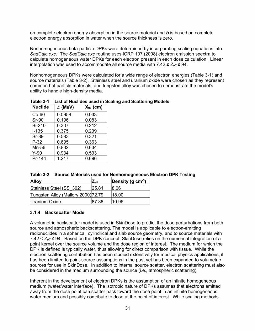
31

on complete electron energy absorption in the source material and b is based on complete electron energy absorption in water when the source thickness is zero. Nonhomogeneous beta-particle DPKs were determined by incorporating scaling equations into SadCalc.exe. The SadCalc.exe routine uses ICRP 107 (2008) electron emission spectra to calculate homogeneous water DPKs for each electron present in each dose calculation. Linear interpolation was used to accommodate all source media with 7.42 ≤ Zeff ≤ 94. Nonhomogeneous DPKs were calculated for a wide range of electron energies (Table 3-1) and source materials (Table 3-2). Stainless steel and uranium oxide were chosen as they represent common hot particle materials, and tungsten alloy was chosen to demonstrate the model’s ability to handle high-density media. Table 3-1 List of Nuclides used in Scaling and Scattering Models Nuclide 𝑬𝑬� (MeV) X90 (cm) Co-60 0.0958 0.033 Sr-90 0.196 0.083 Bi-210 0.307 0.212 I-135 0.375 0.239 Sr-89 0.583 0.321 P-32 0.695 0.363 Mn-56 0.832 0.634 Y-90 0.934 0.533 Pr-144 1.217 0.696

Table 3-2 Source Materials used for Nonhomogeneous Electron DPK Testing Alloy Zeff Density (g cm-3) Stainless Steel (SS_302) 25.81 8.06 Tungsten Alloy (Mallory 2000) 72.79 18.00 Uranium Oxide 87.88 10.96 3.1.4 Backscatter Model

A volumetric backscatter model is used in SkinDose to predict the dose perturbations from both source and atmospheric backscattering. The model is applicable to electron-emitting radionuclides in a spherical, cylindrical and slab source geometry, and to source materials with 7.42 < Zeff ≤ 94. Based on the DPK concept, SkinDose relies on the numerical integration of a point kernel over the source volume and the dose region of interest. The medium for which the DPK is defined is typically water, thus allowing for direct comparison with tissue. While the electron scattering contribution has been studied extensively for medical physics applications, it has been limited to point-source assumptions in the past yet has been expanded to volumetric sources for use in SkinDose. In addition to internal source scatter, electron scattering must also be considered in the medium surrounding the source (i.e., atmospheric scattering). Inherent in the development of electron DPKs is the assumption of an infinite homogeneous medium (water/water interface). The isotropic nature of DPKs assumes that electrons emitted away from the dose point can scatter back toward the dose point in an infinite homogeneous water medium and possibly contribute to dose at the point of interest. While scaling methods

32

account for the nonhomogeneous media that transmit the electrons, an additional adjustment is required to correct for the lack of scatter since an atmospheric medium is above the skin rather than a modeled water medium (i.e., an air/water interface). In the situation of a source resting on the skin, the air above the source (air/water interface) results in less backscatter than would have been modeled in developing the DPKs. This scenario is of particular importance for hot particle skin dosimetry. In the development of the electron dosimetry model (Mangini 2012), point-source planar dose profiles were determined using EGSnrc Monte Carlo simulations for the scattering media of water, air, and source materials with 7.42 < Zeff ≤ 94 at electron energies of 0.01 MeV ≤ E ≤ 8 MeV. The planar dose volumes were 1 mg cm-2 thick, with a maximum normal depth of 1,000 mg cm-2. The dose-averaging areas were 1 cm2 and 10 cm2, consistent with the monitoring areas recommended by ICRP 103 (2007) and National Council on Radiation Protection & Measurement (NCRP) Statement No. 9 (2001), respectively. The scattering medium was assumed infinite (>> electron range) in both thickness and lateral extent. In general, a backscatter factor is found by taking the ratio of the planar dose when the scattering material is present (nonhomogeneous case) to that when water is present (homogeneous case). Air scattering corrections often are reported inversely such that they are greater than or equal to one (1) (Cross et al. 1992). Regardless, these backscatter factors will be dependent on electron energy, the effective atomic number (Z) of the backscattering medium, normal depth, and dose-averaging area. When applied to an electron-emitting nuclide, the backscatter factor for a given dose-averaging area takes the form of

𝐵𝐵𝛽𝛽(𝑍𝑍, 𝑧𝑧) =∫ 𝐷𝐷𝐴𝐴,𝑆𝑆(𝑍𝑍, 𝑧𝑧,𝐸𝐸)𝑁𝑁(𝐸𝐸)𝑑𝑑𝐸𝐸𝐸𝐸𝑚𝑚𝑚𝑚𝑚𝑚0

∫ 𝐷𝐷𝑊𝑊(𝑧𝑧,𝐸𝐸)𝑁𝑁(𝐸𝐸)𝑑𝑑𝐸𝐸𝐸𝐸𝑚𝑚𝑚𝑚𝑚𝑚0

[3.6]

where z is the normal depth, DW is the dose in the water/water geometry, DA,S is either the dose in the air/water geometry or the dose in the source/water geometry, and N(E)dE is the fraction of electrons emitted per MeV per disintegration that have energies between E and E+dE. Surface functions were used to determine monoenergetic electron planar dose profile curve fits for use in Eq. [3.6]. Once planar dose profile curve fits were determined, they were implemented in SadCalc.exe. The ICRP 107 electron-emission spectra were then used to calculate the electron backscatter factor of Eq. [3.6]. Linear interpolation was used for all 7.42 < Z ≤ 94. It is important to remember that it is not possible to determine the absolute volumetric backscatter factor using the same procedures for point sources. This is due to the largely different energy-degradation properties of air and water and their impact on the respective dose calculations. Therefore, several assumptions and estimations were made. The method is based on a selective integration process over the entire source volume. Rather than applying an overall correction factor to final dose calculations, scattering corrections are applied at each step of the numerical integration of dose. If desired, the “volumetric” correction factor could then be determined by taking the ratio of overall dose with the applied point-source scattering corrections to the overall dose without correction. Selection criteria are used to determine the proper type and amount of scattering correction for which to account. Scattering corrections are divided into three components: source/water interface corrections (for the top

33

and bottom of the source), air/water interface corrections (for both the top and the sides of the source), and air/source interface corrections (for the sides of the source). During the numerical integration process for an “infinitely large” source (dimensions > electron range), only source points positioned directly at the source/water interface (i.e., source/skin interface) will require the full application of the source/water scattering data (Figure 3-5). Source points positioned above this interface (Figure 3-6) require a more advanced treatment. In this case, there is expected to be an increase in the energy absorption (i.e., dose) from downward scattering occurring in the upper portion of the source, as well as a decrease in dose from upward scattering in the lower portion of the source. If the contribution from downward scattering is greater than the contribution from upward scattering, the dose will be increased for that source-point kernel. Likewise, when the upward contribution is greater, the dose will be decreased. This argument shows that when the source point is at the top of the source, the application of both air/water and source/water correction results in an effective air/source correction. Scattering contributions from both upward and downward scattering are determined using Eq. [3.7]. The scattering material thicknesses for the top and bottom of the source are given by the normal distances from the source-point to the upper- and lower-most points of the source, respectively. The source backscatter correction factor (BSCF) is then determined by multiplying net scattering effectiveness by the electron source/water scattering correction for point sources,

𝑆𝑆𝑆𝑆𝑆𝑆𝑟𝑟𝑠𝑠𝑠𝑠 𝐵𝐵𝑆𝑆𝐵𝐵𝐹𝐹𝑡𝑡𝑡𝑡𝑡𝑡/𝑏𝑏𝑡𝑡𝑡𝑡𝑡𝑡𝑡𝑡𝑏𝑏 = 𝑆𝑆𝑆𝑆(𝑆𝑆𝐸𝐸𝑡𝑡𝑡𝑡𝑡𝑡 − 𝑆𝑆𝐸𝐸𝑏𝑏𝑡𝑡𝑡𝑡𝑡𝑡𝑡𝑡𝑏𝑏) [3.7] where SW is the electron source/water scattering correction for point-sources, SEtop is the scattering effectiveness for the top portion of the source, and SEbottom is the scattering effectiveness for the bottom portion of the source. The “skin depth” at which the scattering factor is determined accounts for the normal density thickness of both the source and tissue through which the electron must traverse.

Dose Region

Beta-Particle Range

Source Point

Figure 3-5 Schematic Demonstrating Conditions in Which Full Source/Water Scattering

Corrections are Applied

34

Dose Region

Downward Scattering

Upward Scattering

Source PointBeta-Particle Range

Figure 3-6 Schematic Demonstrating Conditions in Which Partial Source/Water Scattering

Corrections are Applied The point-source factors were developed with the assumption that the source medium is infinite in both height and lateral extent. As such, application to source points near or on the side of the source jeopardizes the accuracy of the results. However, approximations can be made to estimate source/scatter corrections for the sides of the source. When the dimensions of the source are larger than the range of the electron, source points toward the center and the top-center of the source have minimal impact on dose. Therefore, source points on both sides and the bottom of the source become more important. It is estimated that scattering contributions from the sides of the source will reach a maximum when the scattering media thickness is 1.0 X/X90 and greater. Linear interpolation is used for X/X90 values less than 1.0. Unlike source scattering for the top and bottom of the source, during the numerical integration process, the direction of the electron needs to be considered when correcting for side scatter. Side scattering is accounted for when the electron’s path is directed away from the source and travels through air before reaching the dose region. The assumption is that an electron emitted in the 180 degree opposite direction would be permitted to backscatter off the source’s side and still contribute to dose. The amount of source material directly above the source point (considered the “lateral” dimension in this case) will also have an impact on the scattering effectiveness. If the source point is located on the top corner of the source, the probability of a backscattering event toward the dose region is greatly decreased. On the other hand, if the source point is at the bottom corner of the source, the probability of a backscattering event toward the dose region is much greater. It is estimated, therefore, that the normal distance to the uppermost point of the source must be greater than 0.5 X/X90 (or ½ of the “height” requirement) to have 100 percent scattering effectiveness from the top portion of the source. Therefore, the net scattering correction is given by 𝑆𝑆𝑆𝑆𝑆𝑆𝑟𝑟𝑠𝑠𝑠𝑠 𝐵𝐵𝑆𝑆𝐵𝐵𝐹𝐹𝑠𝑠𝑠𝑠𝑠𝑠𝑒𝑒 = 𝑆𝑆𝐴𝐴 𝑋𝑋𝑡𝑡𝑡𝑡𝑡𝑡

0.5(𝑋𝑋𝑡𝑡𝑡𝑡_𝑠𝑠𝑠𝑠𝑠𝑠𝑒𝑒 − 𝑋𝑋𝑠𝑠𝑠𝑠𝑠𝑠𝑒𝑒)

[3.8]

where SA is the electron source/air scattering correction for point-sources (ratio of source/water to air/water correction factor), Xside is the normal distance to the side of the source through which the electron travels, Xop_side is the normal distance to the opposite side of the source, and

35

Xtop is the normal distance to the top of the source. All distances are relative to X90. If Xtop is greater than 0.5, the full scattering correction is applied by setting Xtop equal to 0.5. Similarly, if Xside or Xop_side is greater than 1.0, it is set equal to 1.0. As the energy of the electron decreases and the scattered path angle relative to the air/water interface increases, the probability of the scattered electron depositing energy in the dose area greatly decreases (Figure 3-7). Conversely, high-energy electrons are expected to have a contribution extending to the edge of the dose area when scattered electrons enter the dose region at high incident angles. It is assumed that the scattering correction from the top and bottom of the source does not accurately account for such contributions because of its inherent geometry. Without knowing the angle at which a particular electron scatters and likely enters the dose region at each stage of the integration process, it is very difficult to correctly apply this additional correction factor. Therefore, the angle of incident (Figure 3-8) is used to estimate the frequency at which large angle scattering events occur. The side-scattering correction is applied only when the incident angle is greater than 70 degrees and when the density corrected path length (includes source and air) to the edge of the dose region, or the maximum scattered electron path length, is less than the electron X90 distance. The latter limitation prevents the side-scatter correction from being applied to low-energy electrons, where this form of scatter is believed unlikely (as explained above).

High Energy Scattered Beta

Low Energy Scattered BetaSource

Dose Plane

Figure 3-7 Schematic Illustrating Electron Energy Limitations of Side-Scatter Corrections As with scattering from the top or bottom of the source, the “skin depth” at which the scattering factor is determined, considers the normal density thickness of both the source and tissue through which the electron must traverse. The application of scattering correction factors is more difficult with an air/water interface than with a source/water interface. To estimate the scattering effectiveness when source material is present between the air/water interface, simple linear interpolation is used. The two extreme cases are when there is no source material between the air and water boundaries (Figure 3-9) and when the path length from the top or sides of the source is equal to or greater than the electron range. The scattering effectiveness would be 100 percent and 0 percent, respectively. The assumption is that if a backscattered electron can escape the source, there is a chance that a dose-contributing scatter event may still occur if water were surrounding the source. This is seen as a conservative estimate as an electron that travels 1.8 X/X90 (range estimate from US NRC 2006) out of the top of a source will theoretically not be able to backscatter and contribute to skin dose at any depth.

36

Dose Region

Maximum Scattered Beta Path

Incident Beta Path

Source Point

Dose Point

Angle of Incident

Xside Xop_side

Xtop

Figure 3-8 Schematic Illustrating Parameters used to Determine the Amount of Side-

Scatter Correction Applied to High-Energy Electrons Emitted from Large Sources

The overall air BSCF is found using a weighted average. The BSCFs are calculated for all surfaces for which the electron can escape and reach air. Scattering contributions from the top of the source receive a 50 percent weight and the remaining 50 percent is evenly divided among the sides of the source. For cylinders and spheres, the shortest distance to the outer surface and the 180-degree opposite distance represent the two side distances (Figure 3-10). For slabs, four sides are used: the normal distances to the x-coordinate sides and the normal distances to the y-coordinate sides. The scattering reductions (for cylinders and spheres) are therefore given by:

𝐴𝐴𝑑𝑑𝑟𝑟 𝐵𝐵𝑆𝑆𝐵𝐵𝐹𝐹𝑡𝑡𝑡𝑡𝑡𝑡 = 𝐴𝐴𝑆𝑆 0.51.8 − 𝑋𝑋𝑡𝑡𝑡𝑡𝑡𝑡

1.8 [3.9]

𝐴𝐴𝑑𝑑𝑟𝑟 𝐵𝐵𝑆𝑆𝐵𝐵𝐹𝐹𝑠𝑠𝑠𝑠𝑠𝑠𝑒𝑒 = 𝐴𝐴𝑆𝑆 0.251.8 − 𝑋𝑋𝑠𝑠𝑠𝑠𝑠𝑠𝑒𝑒

1.8

[3.10]

and

𝐴𝐴𝑑𝑑𝑟𝑟 𝐵𝐵𝑆𝑆𝐵𝐵𝐹𝐹𝑡𝑡𝑡𝑡_𝑠𝑠𝑠𝑠𝑠𝑠𝑒𝑒 = 𝐴𝐴𝑆𝑆 0.251.8 − 𝑋𝑋𝑡𝑡𝑡𝑡_𝑠𝑠𝑠𝑠𝑠𝑠𝑒𝑒

1.8

[3.11]

where AW is electron air/water scattering correction for point sources, and Xtop, Xside, and Xop_side are the distances to the top and sides of the source relative to X90. Unlike the source scattering corrections, no depth adjustments need to be made for materials traversed by the electron before entering the dose region. This is because corrections are made for scattering events occurring outside the source. The distance to the air/water interface is considered negligible in terms of electron energy degradation (assumed to be completely air). The overall air scattering correction is found by summing the three components above.

37

Figure 3-9 Schematic Demonstrating Conditions in Which Full Air/Water Scattering

Corrections are Applied All profiles were fit with a 28-parameter Chebyshev Series (LnX-Y, Order 6). While this is a complex fit equation, it allowed for all curves to be fit with the same functional form with a high goodness of fit (R2 > 0.999). As an example, a second-order Chebyshev is given by:

𝑍𝑍 = 𝑚𝑚 + 𝑏𝑏𝑇𝑇1(𝑥𝑥′) + 𝑠𝑠𝑇𝑇1(𝐺𝐺′) + 𝑑𝑑𝑇𝑇2(𝑥𝑥′) + 𝑠𝑠𝑇𝑇1(𝐺𝐺′) + 𝑓𝑓𝑇𝑇2(𝐺𝐺′)

[3.12]

where

𝑥𝑥′ = 𝑙𝑙𝑙𝑙( 𝑥𝑥) = 𝑙𝑙𝑙𝑙(𝑁𝑁𝑆𝑆𝑟𝑟𝑚𝑚𝑚𝑚𝑙𝑙 𝐷𝐷𝑠𝑠𝐷𝐷𝐷𝐷ℎ (𝑠𝑠𝑚𝑚)) scaled -1 to +1, 𝐺𝐺′ = 𝐺𝐺 = 𝑙𝑙𝑙𝑙(𝐸𝐸 (𝑀𝑀𝑠𝑠𝑀𝑀)) scaled -1 to +1,

𝑇𝑇𝑛𝑛(𝑥𝑥′) = 𝑠𝑠𝑆𝑆𝑠𝑠(𝑙𝑙 ∗ 𝑚𝑚 ∗ 𝑠𝑠𝑆𝑆𝑠𝑠( 𝑥𝑥′)), and Z is the square root of the dose rate per particle (Gy Bq-1 s-1).

Figure 3-10 Schematic Demonstrating Conditions in Which Air/Water Scattering Corrections

are Applied 3.1.5 Scaling Models

The DPK scaling model consists of two parameters: a depth-scaling parameter (DSP) and an energy-scaling parameter (ESP). Mangini and Hamby (2016) provide more detail.

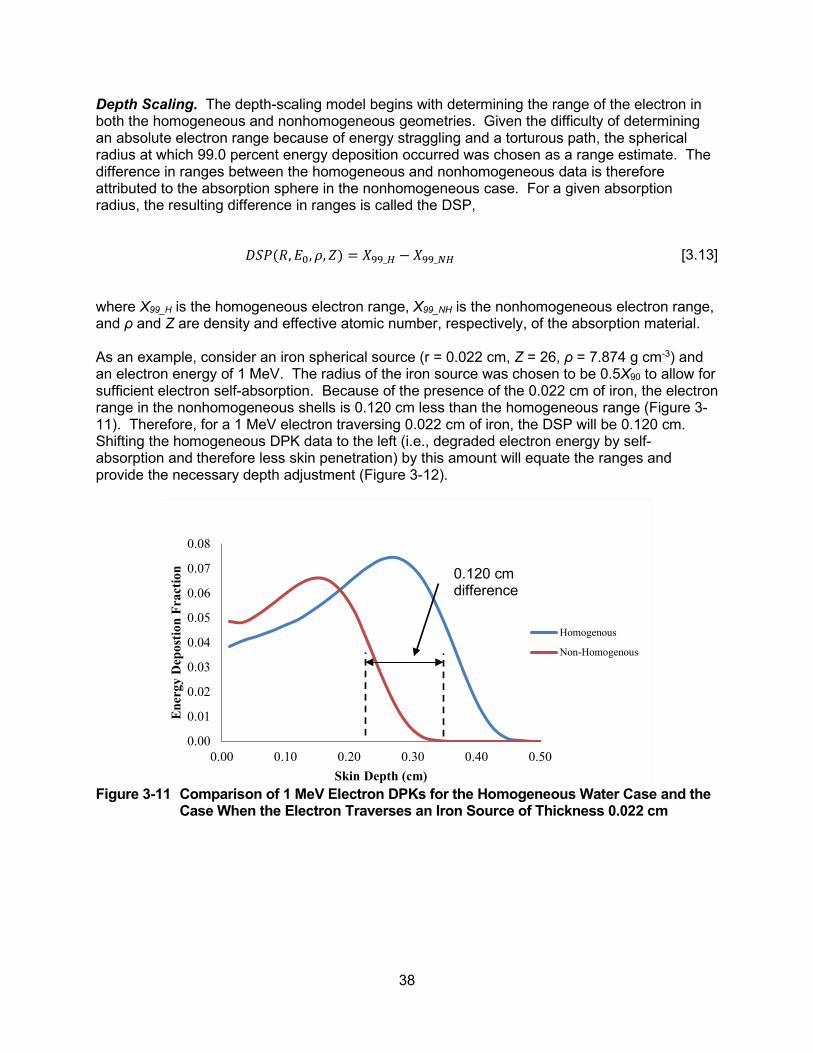
38

Depth Scaling. The depth-scaling model begins with determining the range of the electron in both the homogeneous and nonhomogeneous geometries. Given the difficulty of determining an absolute electron range because of energy straggling and a torturous path, the spherical radius at which 99.0 percent energy deposition occurred was chosen as a range estimate. The difference in ranges between the homogeneous and nonhomogeneous data is therefore attributed to the absorption sphere in the nonhomogeneous case. For a given absorption radius, the resulting difference in ranges is called the DSP,

𝐷𝐷𝑆𝑆𝐸𝐸(𝑅𝑅,𝐸𝐸0,𝜌𝜌,𝑍𝑍) = 𝑋𝑋99_𝐻𝐻 − 𝑋𝑋99_𝑁𝑁𝐻𝐻 [3.13]

where X99_H is the homogeneous electron range, X99_NH is the nonhomogeneous electron range, and ρ and Z are density and effective atomic number, respectively, of the absorption material. As an example, consider an iron spherical source (r = 0.022 cm, Z = 26, ρ = 7.874 g cm-3) and an electron energy of 1 MeV. The radius of the iron source was chosen to be 0.5X90 to allow for sufficient electron self-absorption. Because of the presence of the 0.022 cm of iron, the electron range in the nonhomogeneous shells is 0.120 cm less than the homogeneous range (Figure 3-11). Therefore, for a 1 MeV electron traversing 0.022 cm of iron, the DSP will be 0.120 cm. Shifting the homogeneous DPK data to the left (i.e., degraded electron energy by self-absorption and therefore less skin penetration) by this amount will equate the ranges and provide the necessary depth adjustment (Figure 3-12).

Figure 3-11 Comparison of 1 MeV Electron DPKs for the Homogeneous Water Case and the

Case When the Electron Traverses an Iron Source of Thickness 0.022 cm

0.00

0.01

0.02

0.03

0.04

0.05

0.06

0.07

0.08

0.00 0.10 0.20 0.30 0.40 0.50

Ene

rgy

Dep

ostio

n Fr

actio

n

Skin Depth (cm)

Homogenous

Non-Homogenous

0.120 cm difference

39

Figure 3-12 Example of Depth Scaling on the Homogeneous DPK Curve When plotted together in three dimensions, the variability of depth scaling with respect to Z is difficult to discern, as all DSP factors follow the same curvature with little separation (Figure 3-13). The variation in DSPs at small radii is greatest, with essentially no variability at large radii. Each curve is linear with a slope near unity (1). This is expected since density thickness is often used to estimate “water equivalent” path length for electrons in nonaqueous media. The small Z dependence, coupled with 18 curve fits, allows for accurate interpolation for any 7.42 < Z ≤ 94. All curve fits for the DSPs took the following form:

𝐿𝐿𝑁𝑁(𝐷𝐷𝑆𝑆𝐸𝐸 (𝑠𝑠𝑚𝑚)) =(𝑚𝑚 + 𝑏𝑏𝑥𝑥 + 𝑠𝑠𝑥𝑥2 + 𝑑𝑑𝑥𝑥3 + 𝑠𝑠𝐺𝐺)(1 + 𝑓𝑓𝑥𝑥 + 𝑔𝑔𝑥𝑥2 + ℎ𝑥𝑥3 + 𝑑𝑑𝐺𝐺)

[3.14]

where x is LN(E (MeV)) and y is LN(Xx*ρx (g cm-2)). The terms Xx and ρx refer to the radius and density of the absorption sphere. The form of Eq. [3.14] was chosen because it was the equation that had the largest R2 value (≥0.9999) and was able to fit all 18 plots. The fit parameters for each function demonstrated a slight Z dependence.

0.00

0.01

0.02

0.03

0.04

0.05

0.06

0.07

0.08

0.00 0.10 0.20 0.30 0.40

Ene

rgy

Dep

ostio

n Fr

actio

n

Skin Depth (cm)

Homogenous

Non-Homogenous

40

Figure 3-13 3D Plot of Depth-Scaling Data for all Source Materials Modeled Energy Scaling. The ESP is a direct result of energy conservation at distances within the electron’s maximum range, or X99 (neglecting radiative loses beyond this distance). Once the homogeneous curve is shifted according to the DSP (Figure 3-13), the total energy deposition is found for each case. This is performed by summing the homogeneous DPKs for radii between the depth-scaling parameter and the X99 distance,

4𝜋𝜋𝜌𝜌� 𝑟𝑟2𝛷𝛷(𝑟𝑟,𝐸𝐸0)𝑑𝑑𝑟𝑟 = 𝐸𝐸𝑡𝑡𝑡𝑡𝑡𝑡𝑎𝑎𝑡𝑡𝑋𝑋99

𝐷𝐷𝑆𝑆𝐷𝐷

[3.15]

Similarly, the total energy deposition in the nonhomogeneous case is found by summing DPKs from 0 to X99. The law of energy conservation requires the two to be equal. Therefore, the ESP is found by taking the ratio of the nonhomogeneous total to the homogeneous total, as:

𝐸𝐸𝑆𝑆𝐸𝐸(𝑅𝑅,𝐸𝐸0,𝜌𝜌,𝑍𝑍) =4𝜋𝜋𝜌𝜌∫ 𝑟𝑟2𝛷𝛷𝑁𝑁𝐻𝐻(𝑟𝑟,𝐸𝐸0)𝑑𝑑𝑟𝑟𝑋𝑋99

0

4𝜋𝜋𝜌𝜌∫ 𝑟𝑟2𝛷𝛷𝐻𝐻(𝑟𝑟,𝐸𝐸0)𝑑𝑑𝑟𝑟𝑋𝑋99𝐷𝐷𝑆𝑆𝐷𝐷

[3.16]

Applying the resulting ratio to the homogeneous DPK equates the total energy depositions in the two geometries. For the iron source example, an energy-scaling parameter of 0.887 is computed. Thus, energy conservation is achieved by multiplying the homogeneous curve by the ESP of 0.887 (Figure 3-14).

-5-4

-3-2

-10 1

2

LN(E (MeV))

-15-10

-50

LN(Xx*ρx (g cm-2))

-15 -15

-10 -10

-5 -5

0 0

5 5LN

(DSP

(cm

))

LN(D

SP (c

m))

Depth Scaling for All Materials

41

Figure 3-14 Example of Energy Scaling on the Homogeneous DPK Curve Presented in

Figure 3-13 As in the case of depth scaling, the natural logarithm of energy was used to decrease variability over the range of energies examined. The variability associated with the radius of the absorption sphere was minimized by expressing it as a ratio of density thickness to the X90 distance in water, Xx*ρx / X90w. The natural logarithm of the DSP multiplied by the initial electron energy, LN(ESP*E0), was chosen as the dependent variable. While the quantity of ESP*E0 has no physical meaning, using it as the dependent variable produced better-fitting surface plots than simply using ESP. Since E0 is a known quantity, solving for ESP is simple. The variability of the ESP curves (Figure 3-13) with respect to Z is more pronounced than that of the DSP curves (Figure 3-15). The variation of ESPs becomes quite large as the absorption-sphere radius increases. As Z approaches that of water (Zeff of 7.42), the ESP approaches 1.0, as expected. As Z increases, the amount of energy reduction following depth scaling increases. Once again, this is expected given the lower profile of high-Z nonhomogeneous DPK curves for the same absorption-sphere radius (with respect to X/X90). Despite this increased variability, interpolation within surface plots is not seen as an issue. All curve fits for the ESPs took the form:

𝐿𝐿𝑁𝑁(𝐸𝐸 ∗ 𝐸𝐸𝑆𝑆𝐸𝐸 (𝑀𝑀𝑠𝑠𝑀𝑀)) =(𝑚𝑚 + 𝑏𝑏𝑥𝑥 + 𝑠𝑠𝑥𝑥2 + 𝑑𝑑𝑥𝑥3 + 𝑠𝑠𝐺𝐺 + 𝑓𝑓𝐺𝐺2)

(1 + 𝑔𝑔𝑥𝑥 + ℎ𝑥𝑥2 + 𝑑𝑑𝐺𝐺 + 𝑗𝑗𝐺𝐺2)

[3.17]

where x is LN(E (MeV)) and y is Xx*ρx / X90w. The terms Xx and ρx refer to the radius and density of the absorption sphere. The above equation was chosen because it had the largest R2 value (≥0.999) and was able to fit all 18 plots. As with the DSPs, fit parameters demonstrated a slight Z dependence. Integration of scaling parameters over a particular electron energy spectrum provides the nonhomogeneous DPK for a given source thickness. Comparisons with EGSnrc

0

0.01

0.02

0.03

0.04

0.05

0.06

0.07

0.00 0.10 0.20 0.30 0.40

Ene

rgy

Dep

ostio

n Fr

actio

n

Skin Depth (cm)

Homogenous

Non-Homogenous

42

nonhomogeneous DPKs demonstrated excellent agreement over a range of electron energies and high-Z source materials by producing nearly identical DPKs for all absorption-sphere radii. In addition, when compared to Cross’s (1967, 1968, 1982, 1992) scaling model and density scaling, the ability to account for spectral hardening is evident. This is largely because of the scaling model’s ability to accurately calculate nonhomogeneous DPKs at each monoenergetic electron energy with a given emission spectrum.

Figure 3-15 3D Plot of Energy-Scaling Data for all Source Materials Modeled 3.1.6 Verification and Validation

To validate the new electron dosimetry models incorporated in SkinDose and previous versions of VARSKIN, results were compared to the general-purpose radiation transport codes, Monte Carlo N Particle (MCNP5) and EGSnrc. The two software packages are Monte Carlo transport codes that simulate interaction and transport of particles in material (Los Alamos National Laboratory, 2003; Ljungberg et al. 2012). The authors also compared VARSKIN 5.3 with results from various methodologies in the literature (Anspach and Hamby 2017). Since the unveiling in the late 1980s (US NRC 1987), SkinDose results have been compared with those of many different authors. The following sections provide comparisons with former versions of VARSKIN so that the user can see how dose estimates have changed over the years. In addition, the reader will see comparisons with Monte Carlo simulations, as well as comparisons with results in the literature. Intercode Comparisons. The SkinDose electron dosimetry models have gone through extensive enhancements over their history. Comparisons of dose calculated using VARSKIN 3.1, 4, 5.3, and 6.0 for point sources are given below (using ICRP 38 data for historical consistency) to demonstrate how the four versions differ in dose estimation for the few scenarios considered.

For point sources directly on the skin, calculations were made using several versions of VARSKIN for the case of a Co-60 point source placed directly on the skin (i.e., no material and

-5-4

-3-2

-101

2

LN(E (MeV)) 21.75

1.51.25

10.75

0.50.25

Xx*ρx/X90w

-7 -7-6 -6-5 -5-4 -4-3 -3-2 -2-1 -10 01 12 23 3

LN(E

SP*E

(MeV

))

LN(E

SP*E

(MeV

))

Energy Scaling for All Materials

43

no airgap between the source and skin). For a 37-kBq hot particle and a 1-hour exposure time, the electron dose averaged over 1 cm2 at a depth of 7 mg/cm2 was calculated. Table 3-3 shows the results of this calculation. Changes to electron dosimetry indicate a reduction of about 10 percent at this shallow depth, due primarily to changes in the calculation of specific absorbed dose distribution. Table 3-3 Comparison of Electron Shallow Dose Estimates using VARSKIN 3.1, 4, 5.3, 6.0,

and V+ 1.0 SkinDose for a 37-kBq Point Source of Co-60 on the Skin for 1 hr Nuclide V3.1

β Dose (mGy)

V4 β Dose (mGy)

V5.3 β Dose (mGy)

V6.0 β Dose (mGy)

SkinDose β Dose (mSv)

Co-60 37.6 37.6 34.5 34.5 34 For point sources on cover material, dose calculations at 7 mg/cm2 were also performed for Co-60, Cs-137/Ba-137m, and Sr/Y-90 with three different cover material configurations. In each case, a 37-kBq point source and an exposure time of 1 hour were assumed with no gap between the layers of cover material. Doses were calculated for a 1-cm2 averaging disk. Table 3-4 shows the results of these calculations. Changes to electron dosimetry are shown to either increase or decrease, because of model enhancements that affect particle track lengths, energy loss, backscatter characteristics, conversion electron consideration, and other factors. Table 3-4 Comparison of Electron Shallow Dose Calculations from VARSKIN 3.1, 4, 5.3, 6.0,

and V+ 1.0 SkinDose for Various Cover Material Configurations

Nuclide Airgap (cm)

Cover Material

V3.1 β Dose (mGy)

V4 β Dose (mGy)

V5.3 β Dose (mGy)

V6.0 β Dose (mGy)

SkinDose β Dose (mSv)

Co-60 0.2 M1 1.96 1.96 2.17 2.17 2.2 Cs-137D 0.2 M1 14.0 14.0 13.7 13.5 13 Sr-90D 0.2 M1 32.6 32.6 29.1 28.2 28 Co-60 0.2 2M1 0 0 0.0789 0.0789 0.077 Cs-137D 0.2 2M1 4.75 4.75 6.50 6.44 6.4 Sr-90D 0.2 2M1 20.7 20.7 19.5 19.1 19 Co-60 1.0 M1 0.813 0.813 0.813 0.813 0.81 Cs-137D 1.0 M1 2.79 2.79 2.59 2.53 2.5 Sr-90D 1.0 M1 5.37 5.37 4.74 4.5 Co-60 1.0 2M1 0 0 0.0409 0.0409 0.041 Cs-137D 1.0 2M1 1.40 1.40 1.53 1.49 1.5 Sr-90D 1.0 2M1 3.95 3.95 3.66 3.51 3.5 Co-60 1.0 M1 + M2 0 0 0.00838 0.00838 0.0078 Cs-137D 1.0 M1 + M2 0.770 0.770 1.03 1.01 1.0 Sr-90D 1.0 M1 + M2 3.26 3.26 3.11 3.00 3.0 Co-60 5.0 M1 + M2 0 0 0.00045 0.00045 0.00043 Cs-137D 5.0 M1 + M2 0.0384 0.0384 0.0521 0.0513 0.051 Sr-90D 5.0 M1 + M2 0.167 0.167 0.158 0.153 0.15

Cs-137D includes the progeny Ba-137m; Sr-90D includes the progeny Y-90. M1 — Cover material = thickness of 0.037 cm, density of 0.70 g/cm3 2M1 — Cover material = thickness of 0.074 cm, density of 0.70 g/cm3 M2 — Cover material = thickness of 0.040 cm, density of 1.1 g/cm3 For an infinite plane electron source on the skin, calculations were performed for various nuclides using VARSKIN 4, 5.3, 6.0, and SkinDose to compare specifically the electron dose estimate for a large, distributed disk source (simulating an infinite plane) on the skin for an

44

exposure period of 1 hour (Table 3-5). The electron dose at a depth of 7 mg/cm2 was calculated for a simulated contamination scenario with a total activity of 3.7 MBq (37 kBq/cm2) on a disk source with a diameter of 11.3 cm (100 cm2). A dose-averaging area of 1 cm2 was assumed. Table 3-5 Comparison of VARSKIN 4, 5.3, 6.0, and V+ 1.0 SkinDose of the Electron Dose

(mGy) for a 1-hr Exposure to an Infinite Plane Source on the Skin Nuclide V4 V5.3 V6.0 SkinDose C-14 11.2 11.1 11.1 11 P-32 66.3 58.7 58.7 58 Co-60 37.7 34.5 34.5 35 I-131 52.4 48.4 48.4 48 Cs-137 51.2 47.8 47.8 48 Cs-137D - - 53.5 53 Sr-90 54.7 49.7 49.7 50 Y-90 68.3 59.7 59.7 59 Sr-90D - - 110 110

Cs-137D includes the progeny Ba-137m; Sr-90D includes the progeny Y-90; no dose estimates are given for V4 and V5.3 since those versions did not automatically include decay progeny. Table 3-6 shows additional comparisons at various shallow depths in tissue for a source of yttrium-90 (Y-90). Table 3-6 Dose (mGy) versus Depth for a 37 kBq/cm2 Distributed Disk Source of Y-90 and a

1-hr Exposure Time (Dose Averaged over 1 cm2) Method 4 mg/cm2 7 mg/cm2 10 mg/cm2 40 mg/cm2 VARSKIN 4 79.0 68.3 61.4 40.7 VARSKIN 5.3 65.9 59.7 55.5 38.4 VARSKIN 6.0 65.9 59.7 55.5 38.4 SkinDose 64 59 54 38

Dosimetry Verification and Validation Using Monte Carlo Simulations. MCNP5 and EGSnrc were the two Monte Carlo simulation applications used to compare electron dose calculated in SkinDose. With each application, various source geometries were modeled close to the skin. The fundamental geometry involves an infinite volume of air located above an infinite volume of tissue. Composition of these materials was taken from NIST standards for each material. Each of the sources was situated 1 micron above the skin and above the perpendicular bisect of the volume of tissue over which the dose is calculated.

The dose per particle (electron) was calculated for each of the sources at tissue depths of 7, 100, 300, and 1,000 mg/cm2. The density thicknesses of 7, 300, and 1,000 mg/cm2 correspond to the depth required by 10 CFR Part 20, “Standards for protection against radiation,” for calculation of dose to the skin, lens of the eye, and the deep dose, respectively. Although the value of 100 mg/cm2 does not correspond to a regulatory-significant density thickness, results at that depth are provided as an indication of accuracy at an intermediate, yet shallow, depth. At each density thickness, the dose to two volumes of tissue, 0.002 cm3 and 0.02 cm3, was calculated. These dimensions correspond to cylindrical volumes within tissue, each having a thickness of 20 µm and a cross-sectional area of 1 cm2 and 10 cm2, respectively. The value of 20 µm was selected to create a volume large enough that uncertainties resulting from low numbers of particles interacting in the volume would not be an issue. Sherbini et al. (2008)

45

showed that at thicknesses greater than 10 µm, any effects of dose-averaging over increasingly smaller volumes are avoided. Energy deposited in the volume of interest was calculated for dose estimation. The number of particle histories executed was sufficiently high to maintain statistical errors below 6 percent, with the majority producing an error of approximately 3 percent. Dose rate was calculated for a simulated source strength of 37 kBq, with a yield of 100 percent at a given energy ranging from 0.025 to 3 MeV. While this is not specific to any particular nuclide, it demonstrates the energy dependence of each methodology and shows which models are accurate predictors as compared to Monte Carlo simulations. Previous versions of this NUREG show results of electron dosimetry comparisons arranged in the following seven geometries: (1) point source; (2) 0.5 mm diameter 2D disk source; (3) 1 mm diameter 2D disk source; (4) 5 mm diameter 2D disk source; (5) 1 mm diameter by 1 mm height cylindrical source; (6) 1 mm diameter spherical source; and (7) 1 mm cube slab source. For each geometry, dose estimates from VARSKIN 5 as a function of electron energy were compared with EGSnrc and MCNP5 results at depths of 7, 100, 300, and 1,000 mg/cm2. VARSKIN 5 estimates of dose compare very well with those from EGSnrc and MCNP5, although MCNP5 estimates are slightly higher at deeper depths. Finally, comparisons with four beta-emitting nuclides (Al-28, K-42, Cu-66, and Cs-138) were made to show how VARSKIN 5 electron dose predictions compare to VARSKIN 4 estimates. For additional evidence on the efficacy of SkinDose, the user is directed to two publications in which VARSKIN 5.3 results are compared with historical literature on electron skin dosimetry (Anspach and Hamby 2017; Dubeau et al. 2018). 3.1.7 Limitations

As noted above, the SkinDose validation results indicated differences between VARSKIN 5 and EGSnrc for electron dosimetry in scenarios involving volumetric sources and intermediate electron energies. The validation results for low-energy electrons at shallow depths are similar to the results seen at all depths where the electron is reaching its maximum range (even for the point-sources to a certain degree). These larger deviations are apparent at the tail end of the electron-dose profiles, as well (Mangini, 2012). Either way, it is clear from these results that the accuracy of SkinDose decreases as the electron reaches its maximum depth. In dose calculations for a distribution of electrons, this effect is still present since, approaching the deeper depths, the deposited energy is occurring at the tail end of the electron range. SkinDose has been shown to be reliable for particulate sources that have dimensions less than eight times the X99 distance of the radionuclide in tissue. The X99 distance is essentially 99 percent of the range of beta particles in tissue emitted by nuclides in the source term. When the physical size of the source approaches this value, SkinDose may give unreliable results. A user who wants to model sources larger than this limit may wish to begin with smaller sources and increase the source size gradually to ensure that spurious results are not being generated. Modeling a source of this size is generally not necessary, however, as most of the source does not contribute to electron skin dose because of self-shielding. If the source dimensions selected are too large, SkinDose warns the user of the potential for inaccurate results. The X90 distance is about 56% of X99. X90 is included on the printout of a calculation to assist the user in determining the appropriateness of input source dimensions. As a final note, SkinDose calculates shallow skin dose with the assumption that air is behind the source, i.e., an air/water (simulating tissue) interface at the skin surface. Users are reminded to take care when comparing SkinDose results to other calculations of skin dose that may have

46

been executed with water behind the source (i.e., water/water interface). The BSCF used in SkinDose accounts for this interface difference. DPKs and Scaling Model. DPKs have always underestimated dose at depths approaching the range of the electron. Monte Carlo is the standard and DPK models begin to fail when energy and range straggling become more and more important at greater depths. The effects of straggling are dominant at that part of the electron path. The authors suspect that the scaling model is not a contributor to the discrepancies noted. In fact, the accuracy of the scaling model is highest towards the end of the electron path. The interface between the source material and water is where the model has its largest deviations. This is likely not the cause, as electrons traversing very little of the source material (i.e., 0.25 X/X90) will dominate the dose at deeper depths; the model is extremely accurate in this case.

Scattering Model. In developing the scattering model, the Monte Carlo (EGSnrc) data used for the model all had a standard error less than 5 percent. Simulations with a greater error were eliminated with a dose contribution of zero. However, once the curve fits in SadCalc.exe were developed for the dose profiles, the error in the predicted dose values from the curve fits became extremely unreliable at very low dose values and the deeper depths. In examining the raw data used to create the scattering model and dose profiles, it became apparent that the dose values reached an asymptote of about 1x10-12 (Gy per electron). At these dose values the standard error of the Monte Carlo simulations begins to exceed 5 percents. SkinDose was modified to set all dose contributions to zero if the calculation result was less than 1x10-12 Gy/electron. This patch is justified since the model begins to fail at such low doses. When averaging over a beta spectrum, these contributions to the BSCF and dose are negligible. Setting the dose to zero at these depths is executed for both the source scattering profile and the water scattering profile, thereby setting the BSCF equal to one (1). Nonetheless, for doses just greater than 1x10-12 Gy/electron, the SkinDose model will be rather inaccurate for dose calculations at depths near the end of the electron range.

3.2 Photon Dosimetry

The photon dosimetry model, first implemented in VARSKIN 4 (US NRC 2011), is an improvement to the basic photon model used in the VARSKIN 3 version. The model uses a point kernel method that considers the buildup of CPE, transient CPE, photon attenuation, and off-axis scatter. The photon dose model has many of the basic assumptions carried in the electron dosimetry model, namely that the source can be a point, disk, cylinder, sphere, or slab and that dose is calculated to an averaging disk immediately beneath the skin surface at a depth specified by the user. Photon dose is calculated for a specific skin averaging area, also specified by the user. A major problem associated with deterministic photon dosimetry is determining the amount of charged-particle buildup and electron scatter within shallow depths. Federal law (10 CFR 20.1201(b)) states that a dose-averaging area of 10 cm2 is appropriate for skin dosimetry (specifically at the SDE depth of 0.007 cm in tissue (i.e., 7 mg/cm2 in unit density material)). Throughout this section, the word “depth” is meant to indicate the distance from the skin surface to some point directly beneath a point source, normal to the skin surface. To begin the explanation of the dose model, the simple instance of a volume of tissue exposed to a uniform fluence, Φ0, of uncollided photons of energy, E, from a point source in a homogeneous medium is assumed. When attenuation is ignored and it is assumed that CPE is established, the dose to any and every point in that volume of tissue is:

47

𝐷𝐷(𝐸𝐸) = 𝛷𝛷0 ∙ 𝐸𝐸 ∙ �

𝜇𝜇𝑒𝑒𝑒𝑒𝜌𝜌�𝑡𝑡𝑠𝑠𝑠𝑠𝑠𝑠𝑡𝑡𝑒𝑒

[3.18]

where �𝜇𝜇𝑠𝑠𝑙𝑙

𝜌𝜌�𝐷𝐷𝑑𝑑𝑠𝑠𝑠𝑠𝑆𝑆𝑠𝑠

is the energy-dependent mass energy absorption coefficient for tissue. With

this calculation of dose, it is essentially assumed that the tissue volume is infinitely thin and that interactions occur in two dimensions, normal to a beam of incident photons. The uncollided fluence originating from a point source can be determined by: 𝛷𝛷0 =

𝑆𝑆

4𝜋𝜋𝑑𝑑2 [3.19] where S has units of photons emitted per nuclear transition (i.e., yield), and d is the distance between the source and dose locations, in an infinitely large homogeneous volume. Thus, a point-kernel tissue dose per transition at distance, d, from a point source can be calculated for radionuclides emitting i photons of energy E and yield y, such that:

𝐷𝐷𝑆𝑆𝑠𝑠𝑠𝑠 �Gynt� =

𝑘𝑘� J∙gMeV∙kg�

4𝜋𝜋𝑠𝑠2[cm2] ∙ ∑ �𝐺𝐺𝑠𝑠 �photonnt

� ∙ 𝐸𝐸𝑠𝑠 �MeV

photon� ∙ �𝜇𝜇𝑒𝑒𝑒𝑒

𝜌𝜌�𝑠𝑠,𝑡𝑡𝑠𝑠𝑠𝑠𝑠𝑠𝑡𝑡𝑒𝑒

�cm2

g��𝑠𝑠 [3.20]

where 𝑘𝑘 = 1.602𝑥𝑥10−10 � J∙g

MeV∙kg�.

If the point source is assumed to rest on the skin surface (with a density interface), and a profile of dose with depth in tissue is of interest, Eq. [3.20] must be modified to account for the attenuation of photons in tissue, the electronic buildup, and electron scatter at shallow depths leading to CPE. First, given that attenuation is occurring as photons travel through tissue, photon fluence is decreasing by an attenuation factor (e-µd) where µ is the energy-dependent linear attenuation coefficient for tissue (coefficients are taken from International Commission on Radiation Units and Measurements (ICRU) 44, “Tissue Substitutes in Radiation Dosimetry and Measurement” (ICRU 1989). Since tissue typically is assumed to be of unit density (1 g/cm3), the value of µ (in units of cm-1) is numerically identical to the value of µ/ρ (in units of cm2/g). To simplify software coding, analytical expressions are used in SkinDose (as opposed to using “lookup tables”) for a number of dosimetry parameters. A highly accurate empirical relationship to estimate µ/ρ (in units of cm2/g) for tissue as a function of incident photon energy (in units of MeV) was developed and is given below (Eq. [3.21]). The equation is appropriate for photon energies between 0.001 and 10 MeV.

𝜇𝜇𝜌𝜌

(𝐸𝐸) =𝑚𝑚0 + ∑ 𝑚𝑚𝑠𝑠 ln𝑠𝑠 𝐸𝐸9

𝑠𝑠=1

1 + ∑ 𝑏𝑏𝑠𝑠 ln𝑠𝑠 𝐸𝐸7𝑠𝑠=1

.

[3.21] A similar function was developed (Eq. [3.22]) to approximate the energy-dependent value of µen/ρ for tissue, again appropriate for photon energies between 0.001 and 10 MeV;

𝜇𝜇𝑒𝑒𝑛𝑛𝜌𝜌

(𝐸𝐸) =𝑚𝑚0 + ∑ 𝑚𝑚𝑠𝑠 ln𝑠𝑠 𝐸𝐸7

𝑠𝑠=1

1 + ∑ 𝑏𝑏𝑠𝑠 ln𝑠𝑠 𝐸𝐸8𝑠𝑠=1

.

[3.22]

48

Table 3-7 provides the coefficients for the fit of Eqs. [3.21] and [3.22] to the ICRU 44 (1989) data. In consideration of CPE, Attix (1986) states that the condition exists if, in an infinitely small volume, “…each charged particle of a given type and energy leaving [the volume] is replaced by an identical particle of the same energy entering.” For dose at shallow depths to be accurate, the user must determine the degree (fraction) to which CPE, as a function of depth, has been achieved. The SkinDose estimation of the CPE fraction is based on Monte Carlo simulations and the difference between kinetic energy released in matter (KERMA) and energy absorbed (dose) as a function of depth. Table 3-7 Function Coefficients Coefficient Eq. [3.21] Eq. [3.22] a0 0.06997 0.03067 a1 -0.004154 0.01285 a2 -0.006919 -0.002061 a3 0.001211 -0.001057 a4 0.0005208 0.0003150 a5 -0.00005960 0.0001143 a6 -0.00002192 -0.00001012 a7 0.0000007728 -0.000005314 a8 0.0000007706 - a9 -0.00000002494 - b1 0.4296 0.5972 b2 0.03627 0.1361 b3 -0.005849 0.01239 b4 -0.000006259 -0.0006503 b5 0.0003312 -0.0003667 b6 0.00004527 -0.00005769 b7 0.000001844 -0.000004669 b8 - -0.0000001555

Since energy transfer (i.e., KERMA) from photons and energy absorption (i.e., dose) from the resulting charged particles do not occur in the same location (Johns and Cunningham, 1983), there is a “buildup region” in which dose is zero at the skin surface and then increases until a depth is reached at which dose and KERMA are essentially equal. The depth at which equilibrium occurs is approximately equal to the range of the most energetic electron created by the incident photons (Johns and Cunningham, 1983). The authors determined an energy-dependent factor accounting for CPE buildup (𝑓𝑓𝑐𝑐𝑡𝑡𝑒𝑒) by Monte Carlo simulation (using MCNP5); this factor is the ratio of dose, D, to KERMA, K, for a particular incident photon energy at a given tissue depth; 𝑓𝑓𝑠𝑠𝐷𝐷𝑠𝑠(𝐸𝐸, 𝑑𝑑) = 𝐷𝐷

𝐾𝐾� [3.23] When considering CPE and attenuation, a relationship is achieved with depth in a medium in which dose is proportional to KERMA (Attix 1986); this relationship is referred to as transient charged particle equilibrium (TCPE). Dose reaches a maximum “at the depth where the rising slope due to buildup of charged particles is balanced by the descending slope due to

49

attenuation” (Attix 1986), and then dose continues to decrease with depth because of subsequent attenuation of photons. At the point where TCPE occurs, dose is essentially equal to KERMA for low-energy photons and the value of fcpe is equal to unity (1). As photon energy increases over about 1 MeV, this assumption of dose and KERMA equality begins to fail, but not so significantly that it appreciably affects dose estimations at depth. Based on experience with the Monte Carlo simulation of shallow and deep depths, the model used in SkinDose limits the value of 𝑓𝑓𝑐𝑐𝑡𝑡𝑒𝑒 to 1.05 (i.e., it allows dose to exceed KERMA by no more than 5 percent at depth). A function for 𝑓𝑓𝑐𝑐𝑡𝑡𝑒𝑒 that is dependent on initial photon energy is given as, 𝑓𝑓𝑐𝑐𝑡𝑡𝑒𝑒(𝑥𝑥) = 1

𝑎𝑎+𝑏𝑏𝑡𝑡𝑛𝑛(𝑥𝑥)+𝑐𝑐√𝑥𝑥�

[3.24]

where x (in cm) is a function of energy and is equal to the point kernel distance between source point and dose point, and the coefficients a, b, and c are functions of energy (in keV) as described below: 𝑚𝑚 = 19.78 + 0.1492 𝐸𝐸𝑙𝑙𝑙𝑙𝐸𝐸 − 0.008390 𝐸𝐸1.5 + 0.00003624 𝐸𝐸2 + 3.343 √𝐸𝐸𝑙𝑙𝑙𝑙𝐸𝐸 − 10.72 𝐸𝐸

𝑙𝑙𝑙𝑙𝐸𝐸� [3.25] 𝑏𝑏 = 1.217𝑥𝑥10−12𝐸𝐸4 − 5.673𝑥𝑥10−9𝐸𝐸3 + 7.942𝑥𝑥10−6𝐸𝐸2 − 0.002028𝐸𝐸 + 0.3296 [3.26] 𝑠𝑠 = 9.694𝑥𝑥10−13𝐸𝐸4 − 4.861𝑥𝑥10−9𝐸𝐸3 + 7.765𝑥𝑥10−6𝐸𝐸2 − 0.001856𝐸𝐸 + 0.1467 [3.27] The 𝑓𝑓𝑐𝑐𝑡𝑡𝑒𝑒 factor is used for all materials; any buildup for photon dosimetry in air or thin covers is expected to be insignificant as compared to tissue. 3.2.1 Off-Axis Scatter Correction

Estimates of 𝑓𝑓𝑐𝑐𝑡𝑡𝑒𝑒 were determined assuming that the line created between the source and dose points was normal to the surface. For a given distance, however, the fractional CPE for point kernel calculations, in which the dose point is located off axis and near the edge of the averaging disk, will vary because of the escape of energetic particles near the air-tissue interface. This loss of energy occurs for more energetic particles, generally from photons of energy greater than a few hundred keV. The code accounts for this off-axis scatter of energy out of tissue, slowing the buildup of equilibrium, by including an off-axis scatter factor, Foa. The factor, taking on values between 0 and 1, is necessary only for point-kernel calculations in which the angle between the central axis at the surface and the dose point is greater than 70 degrees from normal, and for photon energies greater than 300 keV; otherwise, Foa is set equal to unity (1). The off-axis scatter factor is calculated from empirical data obtained through Monte Carlo simulation. The factor is represented by, 𝐹𝐹𝑡𝑡𝑎𝑎 = (−1.57 + 0.000334 𝜃𝜃2.5 − 0.0000325 𝜃𝜃3)(0.93 + 0.1𝑅𝑅) [3.28] where R is the radius (cm) of the dose-averaging disk and θ is the off-axis scatter angle (in degrees). Fully accounting for charged particle buildup and attenuation, Eq. [3.20] now becomes: 𝐷𝐷𝑆𝑆𝑠𝑠𝑠𝑠 �𝐺𝐺𝐺𝐺

𝑛𝑛𝑡𝑡� = 𝑘𝑘

4𝜋𝜋𝑠𝑠2∙ ∑ �𝐺𝐺𝑠𝑠 ∙ 𝐸𝐸𝑠𝑠 ∙ �

𝜇𝜇𝑒𝑒𝑒𝑒𝜌𝜌�𝑠𝑠,𝑡𝑡𝑠𝑠𝑠𝑠𝑠𝑠𝑡𝑡𝑒𝑒

∙ �𝑓𝑓𝑐𝑐𝑡𝑡𝑒𝑒�𝑠𝑠 ∙ (𝐹𝐹𝑡𝑡𝑎𝑎)𝑠𝑠 ∙ 𝑠𝑠−𝜇𝜇𝑖𝑖𝑠𝑠�𝑠𝑠 [3.29]

50

3.2.2 Integration Methods

As stated above, Federal law currently requires the determination of shallow dose to skin averaged over an area of 10 cm2 at a depth in tissue of 7 mg/cm2. To determine average photon dose at depth from a source at the surface, Eq. [3.29] must be integrated over the averaging area. Integrating the exponential, however, results in a solution with imaginary components. Therefore, a stepwise numerical integration of Eq. [3.29] is necessary, essentially providing an average of the point-kernel dose over combinations of photon emission locations within the volume of the radioactive source and dose point locations within an infinitely thin disk of tissue at depth, h, from the surface. Studies were conducted to determine which numerical integration method achieved convergence most rapidly (i.e., dividing the dose-averaging disk into the fewest number of segments) for photon dosimetry. The studies investigated three segmenting methods (Figure 3-16): (1) segments determined by equal radii of the dose-averaging disk; (2) segments determined by equal off-axis angles; and (3) segments determined by equal annular area.

Figure 3-16 Depiction of Methods for Determining Integration Segments of the Dose-

Averaging Disk These studies indicate that segments divided according to equal lengths (radii) along the radius of the averaging disk converged with the fewest number of iterations, with segments divided by equal annular area requiring the most iterations. Figure 3-17 shows that convergence was achieved within about 300 iterations for equal lengths along the radius of a 10-cm2 averaging disk; the SkinDose numerical integration, therefore, uses 300 segments along the radius or diameter. Convergence was achieved with fewer segments when analyzing a smaller averaging disk.

51

Figure 3-17 Relative Dose as a Function of the Number of Segments in a Numerical

Integration (Iterations), by Method Therefore, given a point source on the skin, the first task in the integration process is to divide the dose-averaging disk into N small segments (annuli), j, of uniform incremental radii. If an averaging area, A, of radius, R, is at some depth, h, beneath the surface of skin, a method based on the convergence study is used in which values of radii, 𝑅𝑅𝑗𝑗, of the averaging disk are selected such that a radial increment, ∆𝑟𝑟, is defined; ∆𝑟𝑟 = 𝑅𝑅

𝑁𝑁 [3.30]

and 𝑅𝑅𝑗𝑗 = ∑ (𝑗𝑗 ∙ ∆𝑟𝑟)𝑁𝑁

𝑗𝑗=0 [3.31] If point-kernel dose calculations are conducted where dose is estimated to the midpoint of the annulus, each dose must be weighted by 𝑤𝑤𝑗𝑗, the ratio of the annular area to the total area of the disk. Given that R0 = 0 and RN = R, the values of 𝑤𝑤𝑗𝑗 are determined by:

𝑤𝑤𝑗𝑗 =𝑅𝑅𝑗𝑗2−𝑅𝑅𝑗𝑗−1

2

𝑅𝑅2 [3.32]

where j takes on values from 1 to N. Representing the average of the two radii describing the annulus in each calculation, 𝑟𝑟𝑗𝑗 is defined such that; 𝑟𝑟𝑗𝑗 = 𝑅𝑅𝑗𝑗−𝑅𝑅𝑗𝑗−1

2 [3.33]

Once all weighting factors are determined, then the dose per nuclear transition for a given point source radionuclide with i emissions, averaged over an infinitely thin disk of radius R, at normal depth in tissue h and radius 𝑟𝑟𝑗𝑗, is calculated by;

52

�̇�𝐷(ℎ,𝑅𝑅) �Gynt� = 𝑘𝑘

4𝜋𝜋∙ ∑ 𝑤𝑤𝑗𝑗

𝑠𝑠𝑗𝑗2 �∑ �𝐺𝐺𝑠𝑠 ∙ 𝐸𝐸𝑠𝑠 ∙ �

𝜇𝜇𝑒𝑒𝑒𝑒𝜌𝜌�𝑠𝑠∙ �𝑓𝑓𝑐𝑐𝑡𝑡𝑒𝑒�𝑠𝑠,𝑗𝑗 ∙ (𝐹𝐹𝑡𝑡𝑎𝑎)𝑠𝑠,𝑗𝑗 ∙ 𝑠𝑠−𝜇𝜇𝑖𝑖𝑠𝑠𝑗𝑗�𝑠𝑠 �𝑁𝑁

𝑗𝑗=1 [3.34]

where 𝑑𝑑𝑗𝑗 = ��ℎ2 + 𝑟𝑟𝑗𝑗2�. 3.2.3 Attenuation Coefficients for Cover Materials

For the selection of attenuation coefficients in photon dose calculations, the cover materials are “forced” to be either latex or cotton. This determination is made by the density entry, i.e., if the density is less than or equal to 1.25 g/cm3, then latex is assumed, but if the density is greater, cotton is assumed. These are the two most likely materials used for cover. For photons, cover attenuation is relatively minor, and this assumption should be insignificant for the dose calculation. An empirical function of energy for attenuation coefficients for cotton and latex is used, namely: 𝜇𝜇 = 𝑠𝑠(𝑎𝑎+𝑏𝑏√𝐸𝐸∙ln (𝐸𝐸)+𝑐𝑐√𝐸𝐸) [3.35] Coefficients for air were determined from: 𝜇𝜇𝑎𝑎𝑠𝑠𝑟𝑟 = ��𝑚𝑚 + 𝑏𝑏

√𝐸𝐸�+ �𝑠𝑠 ∙ ln(𝐸𝐸)

𝐸𝐸�+ �𝑠𝑠

𝐸𝐸�+ � 𝑒𝑒

𝐸𝐸1.5� + �𝑓𝑓 ∙ ln(𝐸𝐸)𝐸𝐸2

�+ � 𝑔𝑔𝐸𝐸2�� ∗ 0.001168 [3.36]

Table 3-8 contains the coefficients for each equation. Both functions track very closely with data from ICRU 44. Table 3-8 Coefficients for Eqs. [3.35] and [3.36] Coefficient Cotton Latex Air a -0.10132 -1.0286 0.027413 b 0.31505 0.32189 -0.12826 c -1.6086 -1.6217 0.11227 d - - 0.060526 e - - 0.12508 f - - -0.0030978 g - - -0.021571

3.2.4 Off-Axis Calculation of Dose

The model described thus far is constructed under the assumption that the source of photons is a point, located directly above and on axis with the averaging disk, and that there is symmetry in dose calculations along its radius. Dose to the averaging area is calculated for each of 300 annuli defined by radii ri-1 and ri (Figure 3-18) weighted by the annuli area relative to total area.

53

Figure 3-18 Dose-Averaging Disk with the Source Point Located on Axis

To extend the model to handle point-kernel calculations for volumetric sources, or for multiple point sources, the case where the point source is off axis yet still over the dose-averaging disk (Figures 3-19 and 3-20) and the case where the point source is completely removed from the dose-averaging disk (Figures 3-21 and 3-22) must be considered. The implication is simply a geometric determination of the distance between source and dose points in each point-kernel calculation and an area-weighted factor for the symmetric dose location on the averaging disk. In the first case, where the point source is off axis yet still over the dose area, there is symmetry along a diameter of the dose-averaging disk. The average of the point-kernel doses will be determined by a weighting of dose calculated along the diameter. The calculation begins by projecting the dose point to the averaging disk, normal to the skin surface (see Figure 3-19).

Figure 3-19 Dose-Averaging Disk Located at Depth h Beneath an Offset Point Source The averaging disk then is divided, as described above, into a series of concentric annuli, about the projected dose point, until the radius of the annuli reaches the nearest edge of the averaging disk (Figure 3-20). At this point, the weighting model transitions to a series of arcs passing through the averaging disk; these arcs are created by differential radii of two intersecting circles (Figure 3-21). The model creates a total of 300 annuli and arcs. Point kernel dose is calculated

54

along the diameter in each of the 300 segments defined by the differential annuli and arcs and then weighted based on the fractional area of each segment. The weight, or fractional area, of each annulus to the total is straightforward, in that,

𝑤𝑤𝑠𝑠 = 𝜋𝜋�𝑟𝑟𝑖𝑖2−𝑟𝑟𝑖𝑖+1

2 �𝜋𝜋𝑅𝑅2

= 𝑟𝑟𝑖𝑖2−𝑟𝑟𝑖𝑖+1

2

𝑅𝑅2 [3.37]

Figure 3-20 Dose-Averaging Disk with the Source Point Located Off Axis, yet Still Over the Averaging Disk

The weight of each arc is determined by a method considering intersecting circles. In the case of Figure 3-21, the area of the “lens” created by the two intersecting circles is given by: 𝐴𝐴𝑠𝑠 = 𝑟𝑟2𝑠𝑠𝑆𝑆𝑠𝑠−1 �𝑠𝑠

2+𝑟𝑟2−𝑅𝑅2

2𝑠𝑠𝑟𝑟� + 𝑅𝑅2𝑠𝑠𝑆𝑆𝑠𝑠−1 �𝑠𝑠

2+𝑅𝑅2−𝑟𝑟2

2𝑠𝑠𝑅𝑅�

−12�(−𝑑𝑑 + 𝑟𝑟 + 𝑅𝑅)(𝑑𝑑 + 𝑟𝑟 − 𝑅𝑅)(𝑑𝑑 − 𝑟𝑟 + 𝑅𝑅)(𝑑𝑑 + 𝑟𝑟 + 𝑅𝑅) [3.38]

Figure 3-21 Relationship Between the Source-Averaging Disk and One of the Radii for dose Calculation

Dose-averaging disk

Source radii

55

The area of the arc formed (Figure 3-22) by two concentric circles (two radii from the point source) that overlap another circle (the averaging disk) is the difference in the area calculations of Eq. [3.37]. The arc weight is then the ratio of the arc area to the total area of the averaging disk. In the case where the source projection does not fall on the dose-averaging disk (Figure 3-22), the weighting scheme is based solely on arcs. The numerical integration is conducted from the point source to each of 300 locations along the diameter of the averaging disk (or along the radius if the source point is directly on axis with the disk). Then, for volumetric sources, point source locations are chosen in equal symmetric increments at fifteen locations in each of the three dimensions within the source volume, relative to the averaging-disk diameter. For each volumetric source dose estimate, 1,000 calculations of dose from each of 15 x 15 x 15 source point locations are executed (1 million dose calculations). The SkinDose photon dosimetry model accounts for attenuation in cover materials and in air. As with the electron dosimetry model, up to five layers above the skin are allowed, with the air layer only acceptable just above the skin surface. For photon calculations, the material layers are restricted to cotton, latex, or both (by way of attenuation coefficient), and the source material is assumed to have the same characteristics as air. This latter assumption is not significant for very small volumetric sources and for photon energies above about 50 keV. For example, an examination of the ratio of air attenuation to lead, tin, copper, aluminum, and water attenuation, the greatest difference is obviously at low photon energies with higher-Z materials (i.e., instances of higher interaction probability).

Figure 3-22 Dose-Averaging Disk from Above with the Source Point Located Off Axis, far Enough Removed to be Off the Averaging Disk

The data indicate that, for volumetric sources with a maximum linear dimension less than about 100 microns, the assumption that the source material is similar to air is of no consequence whatsoever for photon energies above 10 keV. As the source particle dimensions increase in size, an assumption of air for the source material can be quite significant for very low photon energies (< 40 keV). The significance, however, is one of conservatism in that more low-energy photons than actual will be modeled as striking the skin surface when source dimensions are

56

large. This analysis also shows that, in terms of attenuation, the assumption of air and water (tissue) being similar over very short distances (< 5 mm) is valid. 3.2.5 Verification and Validation

To validate the new photon dosimetry models incorporated into SkinDose and previous versions, results were compared to the general-purpose Monte Carlo radiation transport code MCNP5, which simulates interaction and transport of particles in material (Los Alamos National Laboratory 2003; Ljungberg et al. 2012). VARSKIN 5.3 results were also compared with those from various methodologies in the literature (Anspach and Hamby 2017). Since the unveiling of VARSKIN (SkinDose) in the late 1980s (US NRC 1987), its results have been compared with those of many different authors. The following sections provide comparisons with former versions of SkinDose so that the user can see how dose estimates have changed over the years. In addition to seeing comparisons with Monte Carlo simulation, the reader will be directed to comparisons with the literature. Intercode Comparisons. The SkinDose photon dosimetry models have gone through extensive enhancements over the past several years. Comparisons of dose calculated using VARSKIN 3.1, 4, 5.3, 6.0, and SkinDose for point sources are given below (using ICRP 38 data for historical consistency) to demonstrate how the four versions differ in dose estimation for the few scenarios considered.

For point sources directly on the skin, calculations were made using several versions of SkinDose for the case of a Co-60 point source placed directly on the skin (i.e., no material and no airgap between the source and skin). For a 37-kBq hot particle and a 1-hour exposure time, the photon dose was calculated averaged over 1 cm2 at a depth of 7 mg/cm2. Table 3-9 shows the results of this calculation. Photon dose estimates changed dramatically because of the inclusion of charged particle buildup and photon attenuation. Table 3-9 Comparison of Photon Shallow Dose Estimates using VARSKIN 3.1, 4, 5.3,

6.0, and V+ 1.0 SkinDose for a 37-kBq Point Source of Co-60 on the Skin for 1 hr

Nuclide V3.1 γ Dose (mGy)

V4 γ Dose (mGy)

V5.3 γ Dose (mGy)

V6.0 γ Dose (mGy)

SkinDose γ Dose (mSv)

Co-60 3.29 0.790 0.790 0.790 0.79 For point sources on cover materials, dose calculations at 7 mg/cm2 were also performed for Co-60, Cs-137/Ba-137m, and Sr/Y-90 with three different cover material configurations. In each case, a 37-kBq point source and an exposure time of 1 hour were assumed with no gap between the layers of cover material. Doses were calculated for a 1-cm2 averaging disk. Table 3-10 shows the results of these calculations. Photon dose at shallow depths for the scenario considered decreases by about a factor of two after model enhancement. This is primarily due to the consideration of charged particle buildup and photon attenuation. Using SkinDose for Estimations of Deep Dose Equivalent. In 10 CFR 20.1201, “Occupational dose limits for adults”, reference is made to the deep dose equivalent (DDE). Paraphrasing from 10 CFR 20.1003, “Definitions”, the DDE (Hd) applies to external whole-body exposure and is the dose equivalent at a tissue depth of 1 cm (1,000 mg/cm2). In various nuclear facilities and professions that use radioactive sources, there have been exposure

57

instances in which small, sealed sources are placed in the pockets of clothing and result in potentially large radiation dose to the skin (and underlying organs). SkinDose can be used to calculate dose to a tissue depth of 1 cm, but there is some question whether that result can be expressly applied to represent DDE. Table 3-10 Comparison of Photon Shallow Dose Calculations from VARSKIN 3.1, 4, 5.3,

6.0, and V+ 1.0 SkinDose for Various Cover Material Configurations

Nuclide Airgap (cm)

Cover Material

V3.1 γ Dose (mGy)

V4 γ Dose (mGy)

V5.3 γ Dose (mGy)

V6.0 γ Dose (mGy)

SkinDose γ Dose (mSv)

Co-60 0.2 M1 0.571 0.292 0.290 0.292 0.29 Cs-137D 0.2 M1 0.199 0.0969 0.0959 0.0917 0.099 Sr-90D 0.2 M1 0 0 0 0 - Co-60 0.2 2M1 0.558 0.258 0.257 0.258 0.26 Cs-137D 0.2 2M1 0.181 0.0842 0.0834 0.0797 0.086 Sr-90D 0.2 2M1 0 0 0 0 - Co-60 1.0 M1 0.0797 0.0429 0.0427 0.0429 0.043 Cs-137D 1.0 M1 0.0277 0.0129 0.0128 0.0122 0.013 Sr-90D 1.0 M1 0 0 0 0 - Co-60 1.0 2M1 0.0836 0.0404 0.0402 0.0404 0.040 Cs-137D 1.0 2M1 0.0270 0.0121 0.0121 0.0115 0.013 Sr-90D 1.0 2M1 0 0 0 0 - Co-60 1.0 M1 + M2 0.0876 0.0400 0.0400 0.0400 0.040 Cs-137D 1.0 M1 + M2 0.0271 0.0120 0.0120 0.0114 0.012 Sr-90D 1.0 M1 + M2 0 0 0 0 - Co-60 5.0 M1 + M2 0.0045 0.0020 0.0025 0.0025 0.0020 Cs-137D 5.0 M1 + M2 0.0013 0.0006 0.0006 0.0006 0.00062 Sr-90D 5.0 M1 + M2 0 0 0 0 -

Cs-137D includes the progeny Ba-137m; Sr-90D includes the progeny Y-90. M1 — Cover material = thickness of 0.037 cm, density of 0.70 g/cm3 2M1 — Cover material = thickness of 0.074 cm, density of 0.70 g/cm3 M2 — Cover material = thickness of 0.040 cm, density of 1.1 g/cm3 In 2004, the Electric Power Research Institute (EPRI) released Report #1002823, “Implementing the EPRI Effective Dose Equivalent (EDE) Methodology for Discrete Radioactive Particles on the Skin” (EPRI 2004). The document provides a method of estimating DDE (using MCNP) and states the following:

To calculate DDE at 1 cm depth tissue in this study, a cylindrical-shaped model consisting of tissue equivalent water with cross sectional area of 10 cm2 and a height of 1.2 cm was used. The density of the tissue equivalent water is 1.0 g/cm3, and the composition were based on those by Attix (1986). The isotropic point gamma source was simulated at 10 µm in air above the center of the tissue surface. The DDE is calculated as the dose at 1-cm below the tissue surface to a small disk having 2-mm radius and 70-µm thickness.

To mimic the EPRI estimation of DDE, the following inputs were used with SkinDose: (1) point geometry; (2) dose depth of 10 mm; (3) 1-hour exposure time; (4) 12.6 mm2 averaging area; and (5) 10 µm airgap. Ignoring the 70-µm thickness at a depth of 1 cm will not influence the result. With these inputs, the VARSKIN 6.2.1 results compared very favorably with the EPRI results (see Table 3-11 of the EPRI document):

58

Energy SkinDose V+1.0 EPRI* (MeV) (µSv h-1 MBq-1) (µSv h-1 MBq-1) ========================================= 0.1 98 99.2 0.2 240 242 0.4 550 541 0.6 840 813 Cs-137 790 764 0.662 930 - 0.8 1,100 1,100 1.0 1,300 1,320 1.25 1,600 - Co-60 3,200 3,150 1.5 1,900 1,850 2.0 2,300 2,290 =========================================

*using MCNP The comparison shows that SkinDose provides a photon dose estimate as valid as that provided by an EPRI probabilistic study for estimating DDE for a discrete radioactive particle on the skin. 3.2.6 Limitations

The photon dosimetry model assumes that all volume sources are composed of air. This assumption results in greater accuracy when modeling larger, less dense sources (e.g., a gas cloud). However, when modeling volumetric sources of greater density, SkinDose is optimized for small dimensions (less than about a millimeter). This optimization is the result of a tradeoff between attenuation and charge particle buildup within the source itself. The user should exercise care when modeling large-volume sources (i.e., if the source is large enough to impact self-absorption of photons). 3.3 Alpha Dosimetry

Even at the shallow depth (70 microns), the basal cells in tissue are usually protected from alpha particles on or above the skin because of its dead cellular layer (the stratum corneum). Alpha particles less than about 6.9 MeV will not penetrate this layer, and therefore will not contribute to the SDE. There are, however, a few radionuclides that emit alpha particles of considerable energy, enough to penetrate the dead layer and deposit energy at 70 microns. The alpha dose at a given depth is calculated from the mass stopping power of particles as they pass through the averaging area. The estimate of stopping power begins with the Bragg-Kleeman rule, Λ𝑗𝑗0𝜌𝜌𝑗𝑗�𝑀𝑀𝑎𝑎𝑠𝑠𝑟𝑟 = Λ𝑎𝑎𝑠𝑠𝑟𝑟0 𝜌𝜌𝑎𝑎𝑠𝑠𝑟𝑟 �𝑀𝑀𝑗𝑗,

[3.39]

to determine the linear range, Λ𝑗𝑗0, of an alpha particle in material 𝑗𝑗 given its range in air, Λ𝑎𝑎𝑠𝑠𝑟𝑟0 . As the equation indicates, this relationship is only a function of atomic mass (𝑀𝑀) and density (𝜌𝜌) of

59

material 𝑗𝑗 and air. For the alpha dose calculations in SkinDose, the source is assumed to be a point on the top layer of material regardless of the selected geometry and covers of cotton and latex, an airgap, and tissue thickness are available for energy degradation before the alpha particle reaches the critical depth for SDE (Figure 3-23). Covers with thickness greater than 0.02 cm are assumed to be cotton, whereas those thinner than or equal to 0.02 cm are assumed to be latex. The order of material through which the alpha particle passes is not important and multiple covers may be specified. Table 3-11 gives the values of 𝑀𝑀𝑗𝑗 and 𝜌𝜌𝑗𝑗 for each of the absorbing materials (note that cotton and latex density as specified in Table 3-11 is used for alpha dosimetry and is not taken as the value(s) entered by the user for defining cover characteristics).

Figure 3-23 Diagram of Alpha Source Over the Skin Surface with Cover Materials of

Cotton, Latex, and Air Table 3-11 Material Constants atomic mass, 𝑀𝑀𝑗𝑗 density, 𝜌𝜌𝑗𝑗 Material, 𝑗𝑗 (g/mol) (g/cm3) Air 14.661 0.0012 Cotton 13.294 1.55 Latex 12.591 0.97 Tissue 13.991 1.00

Starting with an initial alpha of energy 𝐸𝐸0, its range through material 𝑗𝑗, Λ𝑗𝑗0, is calculated as:

Λ𝑗𝑗0[𝑠𝑠𝑚𝑚] =�𝑀𝑀𝑗𝑗 𝑀𝑀𝑎𝑎𝑠𝑠𝑟𝑟⁄

𝜌𝜌𝑗𝑗𝐸𝐸𝑋𝑋𝐸𝐸 �

𝑚𝑚 + 𝑏𝑏�𝐸𝐸0 + 𝑠𝑠𝐸𝐸01 + 𝑑𝑑�𝐸𝐸0 + 𝑠𝑠𝐸𝐸0 + 𝑓𝑓𝐸𝐸01.5�,

[3.40] where 𝑀𝑀𝑗𝑗 is the atomic/molecular mass of material 𝑗𝑗, 𝜌𝜌𝑗𝑗 is the bulk density of material 𝑗𝑗, alpha energy is in units of MeV, and the coefficients 𝑚𝑚 through 𝑠𝑠 are given in Table 3-12. The particle is assumed to travel through thickness 𝑙𝑙𝑗𝑗 of material 𝑗𝑗, losing energy and possessing a residual range, Λ𝑗𝑗1𝜌𝜌𝑗𝑗, after passage, such that:

Λ𝑗𝑗1𝜌𝜌𝑗𝑗 �𝑔𝑔𝑠𝑠𝑚𝑚2� = �Λ𝑗𝑗0 − 𝑙𝑙𝑗𝑗� 𝜌𝜌𝑗𝑗.

[3.41]

60

At this point, the residual energy of the alpha particle is

𝐸𝐸1[𝑀𝑀𝑠𝑠𝑀𝑀] = 𝐸𝐸𝑋𝑋𝐸𝐸�𝑚𝑚 + 𝑏𝑏 ln�Λ𝑗𝑗1𝜌𝜌𝑗𝑗� + 𝑠𝑠 ln�Λ𝑗𝑗1𝜌𝜌𝑗𝑗�

2 +𝑑𝑑 ln�Λ𝑗𝑗1𝜌𝜌𝑗𝑗�3

1 + 𝑠𝑠 ln�Λ𝑗𝑗1𝜌𝜌𝑗𝑗� + 𝑓𝑓 ln�Λ𝑗𝑗1𝜌𝜌𝑗𝑗�2 +𝑔𝑔 ln�Λ𝑗𝑗1𝜌𝜌𝑗𝑗�

3 + ℎ ln�Λ𝑗𝑗1𝜌𝜌𝑗𝑗�4�.

[3.42] where coefficients 𝑚𝑚 through ℎ are defined in Table 3-12. The residual energy, 𝐸𝐸1, is now the initial energy available for passing through the next cover layer. The process continues through each layer until the alpha energy is depleted or the dose depth in tissue is reached (e.g., typically 70 microns). At this depth and for the resulting residual energy, the mass stopping power, 𝑆𝑆 𝜌𝜌� , is calculated from

𝑆𝑆𝜌𝜌�𝑀𝑀𝑠𝑠𝑀𝑀 𝑠𝑠𝑚𝑚2

𝑔𝑔� =

𝑚𝑚 + 𝑏𝑏𝐸𝐸1 + 𝑠𝑠𝐸𝐸12 + 𝑑𝑑𝐸𝐸13

1 + 𝑠𝑠𝐸𝐸1 + 𝑓𝑓𝐸𝐸12 + 𝑔𝑔𝐸𝐸13 + ℎ𝐸𝐸14

[3.43] where energy is in units of MeV and the coefficients 𝑚𝑚 through ℎ are in Table 3-12. Table 3-12 Coefficients for Equations Coefficient Eq [3.40] Eq[3.41] Eq[3.42] a -14.553169 4.55197927 306.2468 b -149.01176 1.742181919 15795.781 c -6.1521278 0.229473336 15899.247 d 18.612154 0.010442972 8808.9471 e 2.279749 0.294283366 7.6456075 f 1.3839139 0.030560808 0.57467831 g 0.001341086 8.3211738 h 0.0000312944 1.1392825 The SDE to a receptor location 𝑑𝑑 on an infinitely thin averaging disk is determined from, 𝑆𝑆𝑠𝑠 𝜌𝜌� , the mass stopping power at the receptor using:

𝐷𝐷𝑠𝑠[𝑚𝑚𝑆𝑆𝑚𝑚] = 1.6𝑥𝑥10−7 �𝐽𝐽 𝑔𝑔 𝑚𝑚𝑆𝑆𝑚𝑚

𝑀𝑀𝑠𝑠𝑀𝑀 𝑘𝑘𝑔𝑔 𝑆𝑆𝑚𝑚�𝑆𝑆𝑠𝑠 𝜌𝜌� �𝑀𝑀𝑠𝑠𝑀𝑀 𝑠𝑠𝑚𝑚2

𝑔𝑔� � 𝑤𝑤𝑅𝑅 �𝑆𝑆𝑚𝑚 𝐺𝐺𝐺𝐺� � 𝑄𝑄[𝐵𝐵𝐵𝐵] 𝑌𝑌�𝛼𝛼 𝑙𝑙𝐷𝐷� � 𝐷𝐷[ℎ]

4 𝜋𝜋 𝑙𝑙𝑠𝑠2[𝑠𝑠𝑚𝑚2] .

[3.44] where 𝑤𝑤𝑅𝑅 is the radiation weighting factor, 𝑄𝑄 is the source activity, 𝑌𝑌 is the alpha yield, and 𝐷𝐷 is the time of exposure. The total travel length, 𝑙𝑙𝑠𝑠, from the point source to the point receptor 𝑑𝑑 on the averaging disk (see Figure 3-23), is

𝑙𝑙𝑠𝑠 = �𝑙𝑙𝑗𝑗𝑗𝑗

61

where 𝑙𝑙𝑗𝑗 = ℎ𝑗𝑗cos𝜃𝜃𝑖𝑖

with similar relationships for the other three travel lengths, ℎ𝑗𝑗 is equal to the physical thickness of material 𝑗𝑗, and the angle, 𝜃𝜃𝑠𝑠, in units of radians, is

𝜃𝜃𝑠𝑠 = tan−1 �𝑟𝑟𝑠𝑠−1 + (𝑟𝑟𝑠𝑠 − 𝑟𝑟𝑠𝑠−1)

2ℎ �

where 𝑟𝑟𝑠𝑠 is the radius at point receptor 𝑑𝑑 and ℎ is the total physical thickness of covers, air, and tissue. Alpha dose is calculated at various receptor points along a single radius of the averaging disk (see Figure 3-18), along with an annular weighting (see Eq. [3.32]), to determine total dose to the disk:

𝐷𝐷 = �𝐷𝐷𝑠𝑠 𝑤𝑤𝑠𝑠𝑠𝑠

.

The method incorporated in SkinDose allows estimation of alpha dose equivalent to a given depth in tissue, while also considering the presence of cotton, latex, or air between the source and skin. Simply as a demonstration of this feature, Figure 3-24 shows SkinDose estimates of alpha dose equivalent as a function of depth for two alpha-emitting radionuclides (note instability near the end of the alpha track). The source is modeled as a point on the skin surface assuming an activity of 1 Bq for an exposure time of 1 second, with dose averaged over 10 cm2. Dose results are then in units of dose per nuclear transition. Polonium (Po)-215 emits a 7.4 MeV alpha (99.9-percent yield) and Po-212m emits an 11.7 MeV alpha (96.9-percent yield) with two additional alphas of considerably lower energy. Range in tissue of the high-energy Po-215 and Po-212m alpha particles using a CSDA calculation are 78.5 and 166 microns, respectively. Endpoints determined from the SkinDose alpha dosimetry model for these two nuclides are 73 and 165 microns. 3.4 Cover Layer and Airgap Models

SkinDose has the ability to model cover materials and airgaps. The models use the concept of effective path length to determine the electron energy lost in either a cover material or air before it enters the skin. The path length is not the true path traversed by the electron; rather, it is merely a mathematical convenience introduced to provide a measure of the energy lost in each layer. To minimize unintended applications of SkinDose, the airgap is limited to a maximum of 20 cm. Figure 3-24 illustrates the method used to determine path length within the source and within the cover material. For the pictured cylindrical source, the known values in the figure are the source radius (Rmax), the horizontal distance from the centerline to the source point (SRAD), the source thickness (STHICK), the cover thickness (CTHICK), the skin depth (SDEP), the source and cover densities (Ds and Dc, respectively), the angular distance from the center of the dose area to the dose point (Ps), and the distance from the skin to the plane of the source point (DRAD).

62

Figure 3-24 Schematic of a Generic Dose Calculation Performed by SkinDose for the Cylinder Geometry

The quadrature routines are coded to choose values for SRAD, the distance from the centerline to the Ps source point; θ, the angle between SRAD and Ps; and DRAD, the height of the dose point. The first quantity to be calculated is r, the physical distance from a source point to a dose point. In this calculation, the square of the projected distance, rp

2, is found using the law of cosines: 𝑟𝑟𝑡𝑡2 = 𝐸𝐸𝑠𝑠2 + 𝑆𝑆𝑟𝑟𝑎𝑎𝑠𝑠2 − 2𝐸𝐸𝑠𝑠𝑆𝑆𝑟𝑟𝑎𝑎𝑠𝑠𝑠𝑠𝑆𝑆𝑠𝑠𝜃𝜃 [3.45] The quantity r is used in the denominator of the expression in Eq. [3.1] and represents the geometric attenuation between the dose point and the source point. This quantity is further analyzed to calculate the modified path length used to evaluate the scaled absorbed dose distribution. By the law of similar triangles, the ratio to r of each of the actual distances along r through the source, the cover material, and the tissue is the same as the ratios of the thickness of the cover material to DRAD, the thickness of tissue layer to DRAD, and the remaining distance along r to DRAD respectively, provided that the line connecting the dose point and the source point exits through the part of the source that is in contact with the cover material. Thus, the distance traveled through the cover material is written as the following:

𝑟𝑟𝑐𝑐 = 𝐵𝐵𝑡𝑡ℎ𝑠𝑠𝑐𝑐𝑘𝑘 ∙ �𝑟𝑟 𝐷𝐷𝑟𝑟𝑎𝑎𝑠𝑠� � [3.46]

The distance traveled through the skin is given by:

𝑟𝑟𝑡𝑡 = 𝑆𝑆𝑠𝑠𝑒𝑒𝑡𝑡 ∙ �𝑟𝑟 𝐷𝐷𝑟𝑟𝑎𝑎𝑠𝑠� � [3.47]

and, the distance traveled through the source is given by:

63

𝑟𝑟𝑠𝑠 = �𝐷𝐷𝑟𝑟𝑎𝑎𝑠𝑠 − 𝐵𝐵𝑡𝑡ℎ𝑠𝑠𝑐𝑐𝑘𝑘 − 𝑆𝑆𝑠𝑠𝑒𝑒𝑡𝑡� ∙ �𝑟𝑟 𝐷𝐷𝑟𝑟𝑎𝑎𝑠𝑠� � [3.48]

For electron dosimetry, the modified path length r1 is then found using the following equation:

𝑟𝑟1 = (𝑟𝑟𝑠𝑠𝜌𝜌𝑠𝑠+𝑟𝑟𝑐𝑐𝜌𝜌𝑐𝑐+𝑟𝑟𝑡𝑡𝜌𝜌𝑡𝑡)𝜌𝜌𝑡𝑡

[3.49]

where the variables 𝜌𝜌𝑠𝑠, 𝜌𝜌𝑐𝑐 and 𝜌𝜌𝑡𝑡 represent the density of the source, the cover material, and tissue, respectively. The density of tissue is assumed to be equal to that of water (1 g cm-3). For small-diameter sources, the path between the dose point and the source point may pass through the side of the source (e.g., the path may exit the source and traverse air before passing into skin). Thus, the quantity in Eq. [3.48] must be further analyzed to determine the path length within the source and the path length outside the source but above the level of the cover material. The actual path length within the source is multiplied by the source density, and the path length outside the source and above the cover material is multiplied by the density of the material outside the source, assumed to be air. In spherical geometry, the physical distance from source point to dose point is given by: 𝑟𝑟𝑡𝑡2 = 𝐸𝐸𝑠𝑠2 + 𝑆𝑆𝑟𝑟𝑎𝑎𝑠𝑠2 𝑠𝑠𝑑𝑑𝑙𝑙2𝜙𝜙 − 2𝐸𝐸𝑠𝑠𝑆𝑆𝑟𝑟𝑎𝑎𝑠𝑠𝑠𝑠𝑑𝑑𝑙𝑙𝜙𝜙𝑠𝑠𝑆𝑆𝑠𝑠𝜃𝜃 [3.50] In slab geometry, the physical distance is given by: 𝑟𝑟 = �[(𝑋𝑋𝑠𝑠𝑡𝑡𝑡𝑡𝑟𝑟𝑐𝑐𝑒𝑒 − 𝑋𝑋𝑠𝑠𝑡𝑡𝑠𝑠𝑒𝑒)2 + (𝑌𝑌𝑠𝑠𝑡𝑡𝑡𝑡𝑟𝑟𝑐𝑐𝑒𝑒 − 𝑌𝑌𝑠𝑠𝑡𝑡𝑠𝑠𝑒𝑒)2 + (𝑍𝑍𝑠𝑠𝑡𝑡𝑡𝑡𝑟𝑟𝑐𝑐𝑒𝑒 − 𝑍𝑍𝑠𝑠𝑡𝑡𝑠𝑠𝑒𝑒)2] [3.51] Recent investigations (Anspach and Hamby 2017; McDaniel and Hamby 2017; Dubeau et al. 2018) have shown that the cover and airgap models for electron dosimetry are too conservative (i.e., energy degradation of electrons appears to be too great as they travel through material before entering the skin). The user is cautioned not to rely on SkinDose for source geometries involving cover materials greater than a few centimeters. 3.5 Volume-Averaging Dose Model

The volume-averaging dose model allows the calculation of dose averaged over a given tissue volume. This model works with both photons and electrons yet is only truly meaningful for electron dose calculations. Any two planes of irradiated skin can be assigned to bound the skin volume. For sources in contact with the skin, the maximum penetration depth for electrons is equal to 1.8 times the X90 distance. Doses averaged over the dose-averaging area are calculated at 50 skin depths between two limits set by the user, and a cubic spline (a third-order piecewise polynomial curve fit) is fit to this depth-dose distribution. When the user specifies the skin depths corresponding to the volume of interest, SkinDose integrates the depth dose function over the region of interest to obtain the volume-averaged dose.

65

4 WOUND DOSIMETRY MODEL

NCRP Report No. 156, “Development of a Biokinetic Model for Radionuclide-Contaminated Wounds and Procedures for Their Assessment, Dosimetry, and Treatment” (2007), provides most of the guidance on the wound model as it appears in WoundDose. The wound model consists of three distinct dosimetry calculations: (1) SDE; (2) local dose equivalent; and (3) committed organ/effective dose equivalent. For converting absorbed dose to dose equivalent, the radiation weighting factor, wr, is equal to unity (1) for photons and electrons, and 20 for alpha particles. Total dose is the sum of dose equivalent over the three radiation types. 4.1 Intact Skin, Abrasions and Nonsevere Burns

For contamination events involving less-severe wounds where the skin remains intact, is lightly abraded, or has been lightly burned, dose assessments can be conducted using WoundDose to estimate the SDE calculations in a manner similar to that of SkinDose (i.e., no activity gets in the bloodstream). The shallow dose model is altered only by the removal of some or all of the protective dead layer of skin. NCRP 156 (2007) states the following,

For contaminated wounds in which the skin is largely intact, [VARSKIN] dose calculations may be directly applicable. For embedded contamination, Berger’s point kernels may be integrated over the depth of interest.

Previous versions of VARSKIN (before V5) for beta dosimetry were based on point kernels developed by Berger (1971). The more recent VARSKIN and SkinDose packages (V5.0 and later) have their foundation in Monte Carlo simulations using EGSnrc for electron dosimetry, but the methods are essentially the same. WoundDose draws on the shallow dose model of SkinDose. In 10 CFR 20.1003, shallow skin dose is defined for external exposures and is to be determined at a basal-layer depth of 70 microns (7 mg/cm2, 0.007 cm) beneath the surface of the skin. The basal layer depth varies in human tissue, as does the dead layer of skin, but this depth is assumed to be appropriate for the determination of risk. The regulation in 10 CFR 20.1201 also requires that shallow skin dose be “averaged over the contiguous 10 square centimeters of skin receiving the highest exposure”. If an abrasion were to occur, in which a portion or all of the dead layer of skin were removed, the depth at which shallow dose is determined would be altered by the thickness of removed tissue (alive or dead). With this removal of a portion of the dead layer of skin, Co-60 dose for example to the shallow depth increases for electrons yet decreases for photons. The increase in electron dose is driven by the beta energy distribution and the characteristics of energy loss as a function of penetration depth. The decrease in photon dose is due to a reduction of charged particle buildup in 20 µm as opposed to 70 µm, which is ultimately a function of photon energy.

66

4.2 Severe Burns, Lacerations and Penetrating Wounds

For penetrating wounds where radioactive contamination has been forced under the skin surface, WoundDose will calculate dose for electrons, alpha particles, and photons for all three dose outcomes: (1) shallow dosimetry, which refers to a determination of the dose from the contaminated wound to the shallow basal-cell depth of 70 µm; (2) local dosimetry, which refers to a determination of the dose to tissue surrounding the contaminated wound; and (3) committed systemic dosimetry for uptakes to the bloodstream, which potentially affects all organs of the body. For estimates of local dose, particle/photon energy emitted from a point source is assumed to be deposited in a standard spherical volume of 1 cm3 (radius = 0.62 cm). For a line source, the deposition volume is assumed to be a cylinder of radius 0.62 cm with hemispherical endcaps (NRCP 2007). Calculations of shallow and local dose in WoundDose are conducted for an estimated time that the radioactive contamination remains at the wound site (e.g., residence time). This residence time is determined by time-integrating the retention function

𝜏𝜏 = � 𝑠𝑠−𝜆𝜆𝑒𝑒𝑡𝑡 𝑑𝑑𝐷𝐷∞

0=

1𝜆𝜆𝑒𝑒

where 𝜆𝜆𝑒𝑒 is equal to the sum of the radiological decay constant and the rate constant for biological loss. WoundDose employs the user-defined estimate of biological half-life from its selection of retention class. The “avid” retention class, for example, shows a biological half-life of 560 days. If the radionuclide contaminant in the wound has a radiological half-life of 2.5 years (912 days), the effective loss constant is

𝜆𝜆𝑒𝑒 =ln(2)

560 [𝑑𝑑] +ln(2)

912 [𝑑𝑑] = 0.002 [𝑑𝑑−1]

with a wound residence time of 500 days. The residence time is used as the exposure time for calculating total dose at the shallow tissue depth and for the local dose sphere. Additional information on the three dose calculations follows. 4.3 Shallow Dosimetry

To estimate total dose at the shallow depth (7 mg/cm2) with an embedded wound source, the models of SkinDose are accessed, but with modified backscatter correction. The calculations are otherwise identical. In addition to the typical skin dosimetry inputs, the user would enter the thickness of any surface tissue that might have been removed by the wound, as well as the wound retention class (e.g., weak, moderate, strong), and an estimate of its penetration depth. Point Source at Depth. In this case, the distance between source and skin averaging area is determined by the difference between source depth and the defined shallow depth (7 mg/cm2). The user should still have the option to select the depth at which dose is calculated, but 7 mg/cm2 would remain as the default. Line Source Surface to Depth. In this instance, it is assumed that a puncture has occurred (e.g., contaminated screwdriver) and any remnant of contamination is evenly distributed along the puncture route. The shallow dose at 7 mg/cm2 to a specified skin averaging area (10 cm2) is calculated under the assumption that the line source begins at the surface, possibly penetrates

67

the averaging area, and continues to the user-specified wound depth. The problem in this case requires the numerical integration of dose over a series of point sources at depth, along the wound penetration line. The penetrating wound is assumed to be perpendicular to the skin surface. 4.4 Local Dosimetry

Local dosimetry refers to estimating the dose equivalent to the tissue surrounding the contaminated wound volume. That contamination may exist as a point (hot particle; modeled as a point source) at some depth following penetration, or it may be spread from the entry location along the entire length of the wound to a final penetration depth (modeled as a line source perpendicular to the surface of the skin). If a puncture wound results in a hot particle or point source at some depth in tissue, the local dose calculation is made assuming energy deposition occurs in a 1 cm3 sphere centered on the point source. All electron and alpha energy is assumed to be absorbed in that volume and a fraction of photon energy is calculated for absorption. Electrons. For a point source beneath the skin surface, the local dose due to electrons is:

𝐷𝐷𝑒𝑒 = 𝑠𝑠𝑄𝑄 𝜏𝜏 𝑤𝑤𝑟𝑟𝑒𝑒 𝑌𝑌 𝐸𝐸�

𝜌𝜌 𝑀𝑀𝐷𝐷

where 𝑠𝑠 handles unit conversion, 𝑄𝑄 is the activity initially introduced into the wound, 𝜏𝜏 is residence time, 𝑤𝑤𝑟𝑟𝑒𝑒 is unity for electrons, 𝑌𝑌 is electron emission yield, 𝐸𝐸� is average electron energy (considering all beta and electron emissions), 𝜌𝜌 is tissue density, and 𝑀𝑀𝐷𝐷 is the absorption volume (1 cm3). Alphas. The local dose due to alpha emissions is:

𝐷𝐷𝛼𝛼 = 𝑠𝑠𝑄𝑄 𝜏𝜏 𝑤𝑤𝑟𝑟𝛼𝛼𝜌𝜌 𝑀𝑀𝐷𝐷

�𝑌𝑌𝑠𝑠 𝐸𝐸𝑠𝑠𝑠𝑠

where 𝑤𝑤𝑟𝑟𝛼𝛼 is 20 for alpha particles and 𝐸𝐸𝑠𝑠 is the energy of the ith alpha with yield 𝑌𝑌𝑠𝑠. Photons. The photon dose for an embedded point source is calculated for energy deposited in a surrounding 1 cm3 sphere, using:

𝐷𝐷𝛾𝛾 = 𝑠𝑠𝑄𝑄 𝜏𝜏 𝑤𝑤𝑟𝑟𝛾𝛾𝜌𝜌 𝑀𝑀𝐷𝐷

�𝑌𝑌𝑠𝑠 𝐸𝐸𝑠𝑠 𝑓𝑓𝑠𝑠𝑠𝑠

where w is unity for photons, and the fraction of photon energy deposited within a sphere of radius r (0.62 cm) around the source (Piechowski and Chaptinel, 2004) is:

𝑓𝑓𝑠𝑠 =(𝜇𝜇𝑒𝑒𝑛𝑛)𝑠𝑠𝜇𝜇𝑠𝑠

(1 − 𝑠𝑠−𝜇𝜇𝑖𝑖𝑟𝑟)

68

with 𝜇𝜇𝑒𝑒𝑛𝑛 and 𝜇𝜇𝑠𝑠 representing energy-specific linear absorption and attenuation coefficients in tissue, respectively. A line source is handled in the same fashion with one exception. In this case, the volume of tissue in which energy is deposited is:

𝑀𝑀𝐿𝐿 = 𝜋𝜋𝑟𝑟2 (𝐿𝐿 + 1.33𝑟𝑟) where 𝐿𝐿 is the length (i.e., depth of the wound) and 𝑟𝑟 is the radius (0.62 cm) of the cylinder surrounding the line source, including two hemispherical end caps. Dose calculated for a point source can be converted to dose from a line source with a simple ratio of volumes. For example, an injury depth of 5 mm results in a dose ratio of:

𝐷𝐷𝐿𝐿𝐷𝐷𝐷𝐷

=𝑀𝑀𝐷𝐷𝑀𝑀𝐿𝐿

=1

1.6= 0.63

where subscripts 𝐿𝐿 and 𝐸𝐸 refer to the line source and point source, respectively. 4.5 Systemic Dosimetry

The biokinetic model for radiologically contaminated wounds considers four uptake categories: (1) radionuclides in soluble form; (2) particulates, aggregates, and bound states; (3) colloid and intermediate states; and (4) fragments. Movement of material from the wound and through the body to the bloodstream is characterized by the biokinetic model in Figure 4-1 (NCRP 2007).

Figure 4-1 General Compartment Model of the Biokinetics of Radionuclides

and/or Radioactive Materials Deposited in a Wound (taken from NCRP 156)

Others (including Toohey et al. 2014) have tabulated internal dose coefficients for radionuclides reaching the bloodstream via penetrating wounds. WoundDose uses these dose coefficients to estimate internal dose equivalent via absorption following a skin wound. The coefficients vary based on nuclide and on the solubility of the molecular form in which the nuclide is incorporated. Dose coefficients account for a subcutaneous or intramuscular injection that may enter the bloodstream directly from the injection site. An examination of coefficients indicates that effective dose could vary by two orders of magnitude depending on the chemical/physical form

69

of the compound containing the radioactivity. The user of WoundDose should refer to NCRP 156 (NCRP 2007) to determine the solubility characteristics of the chemical form in which the radionuclide is introduced. WoundDose estimates dose for all seven solubility characteristics provided by the NCRP 156 model. If the user selects the “Custom” feature for biological half-life at the wound site, WoundDose chooses the retention class with the nearest biological half-life to that entered.

71

5 NEUTRON DOSIMETRY MODEL

A new feature in VARSKIN+ is the addition of a neutron dosimetry model. Consideration is made for neutron interactions from thermal (10-11 MeV min.) to fast (20 MeV max.), where a set of KERMA values can be generated using neutron interaction equations. The depth-dose equations can then be applied to these values for an estimate of neutron dose at a specific depth. This is especially important for incident neutrons above 1 MeV where charged particle KERMA is not equivalent to dose at shallow depths. This culminates in a neutron dose model in which the shallow skin dose from a monoenergetic neutron can be determined simply through the input of the neutron’s energy, fluence, and tissue depth. The generalized shallow neutron dosimetry model applied in NeutronDose is:

𝐻𝐻(𝑑𝑑,𝐸𝐸) = 𝑤𝑤𝑟𝑟(𝐸𝐸) ∙ 𝐾𝐾(𝑑𝑑,𝐸𝐸) ̇ ∙ 𝑓𝑓𝑐𝑐𝑡𝑡𝑒𝑒(𝑑𝑑,𝐸𝐸) [5.1] where 𝐻𝐻(𝑑𝑑,𝐸𝐸) is the equivalent dose at a specific depth in tissue for a given neutron energy relative to a perpendicular fluence of neutrons to the tissue surface. The radiation weighting factor for a given neutron at a specific energy is given by 𝑤𝑤𝑟𝑟(𝐸𝐸). The neutron KERMA at depth 𝑑𝑑 for incident energy 𝐸𝐸 is 𝐾𝐾(𝑑𝑑,𝐸𝐸), and 𝑓𝑓𝑐𝑐𝑡𝑡𝑒𝑒(𝑑𝑑,𝐸𝐸) is the depth- and energy-dependent fractional charged particle equilibrium (CPE). 5.1 Neutron Source Term

The neutron dose module provides dosimetry for six different source types: (1) spontaneous fission; (2) neutron-induced fission; (3) alpha reaction neutrons (α,n); (4) photoneutrons (γ,n); (5) a monoenergetic neutron; and (6) a user-uploaded custom energy distribution. Both spontaneous fission and neutron-induced fission sources use the Watt fission spectrum equation:

𝜒𝜒(𝐸𝐸) = 𝐵𝐵𝑟𝑟�̅�𝜈 exp �−𝐸𝐸𝐴𝐴� sinh�√𝐵𝐵𝐸𝐸�

The values 𝐴𝐴 and 𝐵𝐵 are taken from ICRP 107 for spontaneous fission sources, and from Shultis and Faw (2000) for neutron-induced fission as a function of incident neutron energy, 𝐸𝐸, up to a maximum of 10 MeV. The leading coefficients, 𝐵𝐵𝑟𝑟 and �̅�𝜈, represent the branching ratio and average number of neutrons produced per fission for spontaneous fission events (Table 5-1). For neutron-induced fission these two coefficients (Table 5-2) are based on a method by Walsh (1989); the user is further directed to Shultis and Faw (2000) and cautioned that, although used in the same form of the equation above, the coefficients 1 and 2 (Table 5-2) do not relate to branching ratio or neutrons per fission. Neutron dose is integrated across the energy spectrum calculated from exposure time, distance to the source, and activity of the selected spontaneous fission source. Neutron-induced fission dose is calculated based on the total neutron fluence provided as user input.

72

Table 5-1 χ(E) Data for Nuclides which Spontaneously Fission (ICRP 107)

Table 5-2 χ(E) Data for Neutron-Induced Fission (Shultis & Faw 2000) Nuclide Coeff 1 Coeff 2 A B U-233 0.86159 0.70520 0.903 1.26 U-235 0.84180 0.65749 0.962 1.62 Pu-239 0.81547 0.70023 0.863 1.23 Th-232 0.87263 0.64188 1.030 1.83 U-238 0.86327 0.66700 0.974 1.58

Six alpha reaction sources can be modeled by Varskin+, including: (1) AmB; (2) AmBe; (3) AmF; (4) CmBe; (5) PuBe; and (6) PuC. Characteristics of these reactions are given in Table 5-3.

Nuclide Fissions/decay (𝐵𝐵𝑟𝑟) Neutrons/fission (�̅�𝜈) A B U-238 5.45E-7 2.01 0.648 6.81 Pu-236 1.37E-9 2.13 0.998 3.10 Pu-238 1.85E-9 2.22 0.848 4.17 Pu-240 5.75E-8 2.16 0.795 4.69 Pu-242 5.54E-6 2.15 0.819 4.37 Pu-244 1.21E-3 2.30 0.695 6.00 Cm-240 3.90E-8 2.39 1.072 2.70 Cm-242 6.37E-8 2.52 0.887 3.89 Cm-244 1.37E-6 2.69 0.903 3.72 Cm-245 6.10E-9 2.87 0.912 3.62 Cm-246 2.63E-4 3.18 0.878 3.89 Cm-248 8.39E-2 3.11 0.808 4.54 Cm-250 7.40E-1 3.31 0.734 5.44 Cf-246 2.50E-6 3.10 1.026 2.93 Cf-248 2.90E-5 3.34 1.028 2.93 Cf-249 5.02E-9 3.41 1.026 2.93 Cf-250 7.70E-4 3.53 1.026 2.93 Cf-252 3.09E-2 3.77 1.025 2.93 Cf-254 9.97E-1 3.89 1.026 2.93 Es-253 8.90E-8 3.93 0.820 4.60 Es-254 3.00E-8 3.95 0.820 4.60 Es-254m 4.50E-4 3.95 0.820 4.60 Es-255 4.50E-5 3.97 0.820 4.60 Fm-252 2.30E-5 3.90 0.820 4.60 Fm-255 2.30E-7 3.73 0.820 4.60 Fm-256 9.19E-1 4.01 0.820 4.60 Fm-257 2.10E-3 3.85 0.820 4.60

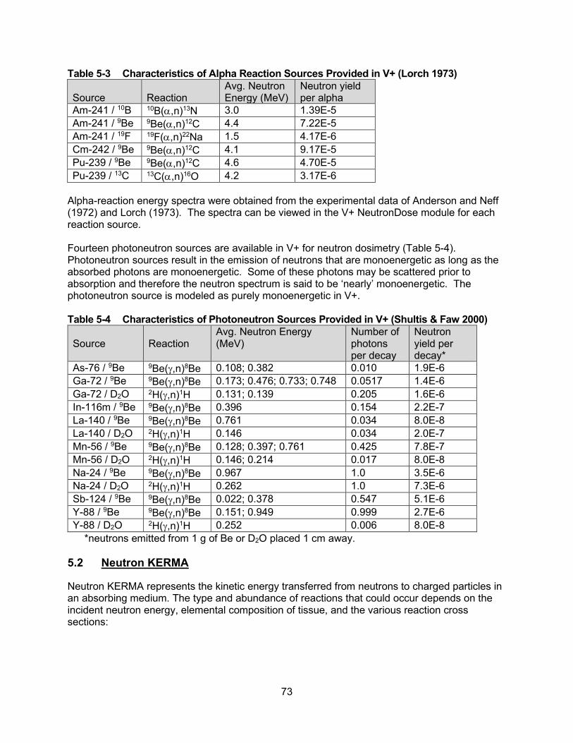
73

Table 5-3 Characteristics of Alpha Reaction Sources Provided in V+ (Lorch 1973) Source

Reaction

Avg. Neutron Energy (MeV)

Neutron yield per alpha

Am-241 / 10B 10B(α,n)13N 3.0 1.39E-5 Am-241 / 9Be 9Be(α,n)12C 4.4 7.22E-5 Am-241 / 19F 19F(α,n)22Na 1.5 4.17E-6 Cm-242 / 9Be 9Be(α,n)12C 4.1 9.17E-5 Pu-239 / 9Be 9Be(α,n)12C 4.6 4.70E-5 Pu-239 / 13C 13C(α,n)16O 4.2 3.17E-6

Alpha-reaction energy spectra were obtained from the experimental data of Anderson and Neff (1972) and Lorch (1973). The spectra can be viewed in the V+ NeutronDose module for each reaction source. Fourteen photoneutron sources are available in V+ for neutron dosimetry (Table 5-4). Photoneutron sources result in the emission of neutrons that are monoenergetic as long as the absorbed photons are monoenergetic. Some of these photons may be scattered prior to absorption and therefore the neutron spectrum is said to be ‘nearly’ monoenergetic. The photoneutron source is modeled as purely monoenergetic in V+. Table 5-4 Characteristics of Photoneutron Sources Provided in V+ (Shultis & Faw 2000) Source

Reaction

Avg. Neutron Energy (MeV)

Number of photons per decay

Neutron yield per decay*

As-76 / 9Be 9Be(γ,n)8Be 0.108; 0.382 0.010 1.9E-6 Ga-72 / 9Be 9Be(γ,n)8Be 0.173; 0.476; 0.733; 0.748 0.0517 1.4E-6 Ga-72 / D2O 2H(γ,n)1H 0.131; 0.139 0.205 1.6E-6 In-116m / 9Be 9Be(γ,n)8Be 0.396 0.154 2.2E-7 La-140 / 9Be 9Be(γ,n)8Be 0.761 0.034 8.0E-8 La-140 / D2O 2H(γ,n)1H 0.146 0.034 2.0E-7 Mn-56 / 9Be 9Be(γ,n)8Be 0.128; 0.397; 0.761 0.425 7.8E-7 Mn-56 / D2O 2H(γ,n)1H 0.146; 0.214 0.017 8.0E-8 Na-24 / 9Be 9Be(γ,n)8Be 0.967 1.0 3.5E-6 Na-24 / D2O 2H(γ,n)1H 0.262 1.0 7.3E-6 Sb-124 / 9Be 9Be(γ,n)8Be 0.022; 0.378 0.547 5.1E-6 Y-88 / 9Be 9Be(γ,n)8Be 0.151; 0.949 0.999 2.7E-6 Y-88 / D2O 2H(γ,n)1H 0.252 0.006 8.0E-8

*neutrons emitted from 1 g of Be or D2O placed 1 cm away. 5.2 Neutron KERMA

Neutron KERMA represents the kinetic energy transferred from neutrons to charged particles in an absorbing medium. The type and abundance of reactions that could occur depends on the incident neutron energy, elemental composition of tissue, and the various reaction cross sections:

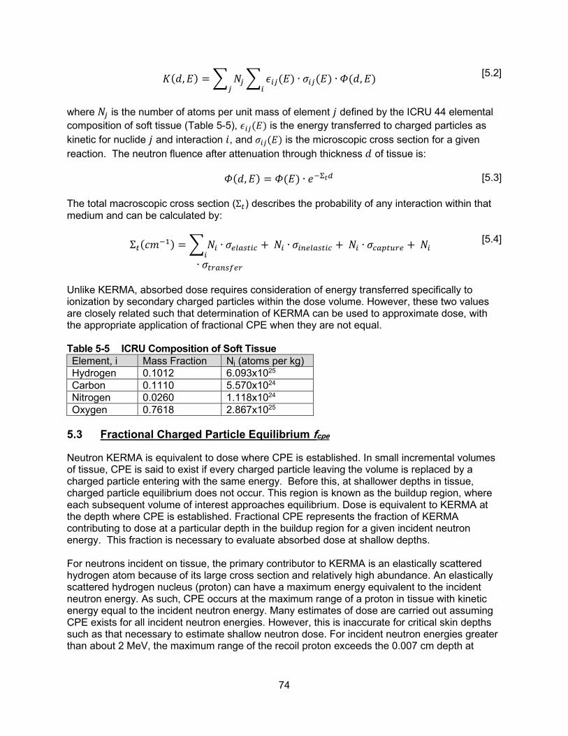
74

𝐾𝐾(𝑑𝑑,𝐸𝐸) = � 𝑁𝑁𝑗𝑗𝑗𝑗

� 𝜖𝜖𝑠𝑠𝑗𝑗(𝐸𝐸) ∙ 𝜎𝜎𝑠𝑠𝑗𝑗(𝐸𝐸) ∙ 𝛷𝛷(𝑑𝑑,𝐸𝐸)𝑠𝑠

[5.2]

where 𝑁𝑁𝑗𝑗 is the number of atoms per unit mass of element 𝑗𝑗 defined by the ICRU 44 elemental composition of soft tissue (Table 5-5), 𝜖𝜖𝑠𝑠𝑗𝑗(𝐸𝐸) is the energy transferred to charged particles as kinetic for nuclide 𝑗𝑗 and interaction 𝑑𝑑, and 𝜎𝜎𝑠𝑠𝑗𝑗(𝐸𝐸) is the microscopic cross section for a given reaction. The neutron fluence after attenuation through thickness 𝑑𝑑 of tissue is: 𝛷𝛷(𝑑𝑑,𝐸𝐸) = 𝛷𝛷(𝐸𝐸) ∙ 𝑠𝑠−Σ𝑡𝑡𝑠𝑠 [5.3]

The total macroscopic cross section (Σ𝑡𝑡) describes the probability of any interaction within that medium and can be calculated by: Σ𝑡𝑡(𝑠𝑠𝑚𝑚−1) = �𝑁𝑁𝑠𝑠 ∙ 𝜎𝜎𝑒𝑒𝑡𝑡𝑎𝑎𝑠𝑠𝑡𝑡𝑠𝑠𝑐𝑐

𝑠𝑠+ 𝑁𝑁𝑠𝑠 ∙ 𝜎𝜎𝑠𝑠𝑛𝑛𝑒𝑒𝑡𝑡𝑎𝑎𝑠𝑠𝑡𝑡𝑠𝑠𝑐𝑐 + 𝑁𝑁𝑠𝑠 ∙ 𝜎𝜎𝑐𝑐𝑎𝑎𝑡𝑡𝑡𝑡𝑡𝑡𝑟𝑟𝑒𝑒 + 𝑁𝑁𝑠𝑠

∙ 𝜎𝜎𝑡𝑡𝑟𝑟𝑎𝑎𝑛𝑛𝑠𝑠𝑡𝑡𝑒𝑒𝑟𝑟

[5.4]

Unlike KERMA, absorbed dose requires consideration of energy transferred specifically to ionization by secondary charged particles within the dose volume. However, these two values are closely related such that determination of KERMA can be used to approximate dose, with the appropriate application of fractional CPE when they are not equal. Table 5-5 ICRU Composition of Soft Tissue Element, i Mass Fraction Nj (atoms per kg) Hydrogen 0.1012 6.093x1025 Carbon 0.1110 5.570x1024 Nitrogen 0.0260 1.118x1024 Oxygen 0.7618 2.867x1025

5.3 Fractional Charged Particle Equilibrium fcpe

Neutron KERMA is equivalent to dose where CPE is established. In small incremental volumes of tissue, CPE is said to exist if every charged particle leaving the volume is replaced by a charged particle entering with the same energy. Before this, at shallower depths in tissue, charged particle equilibrium does not occur. This region is known as the buildup region, where each subsequent volume of interest approaches equilibrium. Dose is equivalent to KERMA at the depth where CPE is established. Fractional CPE represents the fraction of KERMA contributing to dose at a particular depth in the buildup region for a given incident neutron energy. This fraction is necessary to evaluate absorbed dose at shallow depths. For neutrons incident on tissue, the primary contributor to KERMA is an elastically scattered hydrogen atom because of its large cross section and relatively high abundance. An elastically scattered hydrogen nucleus (proton) can have a maximum energy equivalent to the incident neutron energy. As such, CPE occurs at the maximum range of a proton in tissue with kinetic energy equal to the incident neutron energy. Many estimates of dose are carried out assuming CPE exists for all incident neutron energies. However, this is inaccurate for critical skin depths such as that necessary to estimate shallow neutron dose. For incident neutron energies greater than about 2 MeV, the maximum range of the recoil proton exceeds the 0.007 cm depth at

75

which shallow dose is determined. Absorbed dose for energies greater than 2 MeV, therefore, is only a fraction of KERMA at the shallow depth. For relatively short range (< 350 microns) recoil protons from incident neutrons less than 5 MeV, tissue segments were simulated at thicknesses of 5 microns. The following function was developed from the MCNP results and is applicable for neutron energies between 1 and 5 MeV: 𝑓𝑓𝑐𝑐𝑡𝑡𝑒𝑒(𝐸𝐸,𝑑𝑑) = 𝐴𝐴 + 𝐵𝐵(10𝑑𝑑) + 𝐵𝐵(10𝑑𝑑) ∗ ln(10𝑑𝑑) [5.5]

where 𝑑𝑑 is the tissue depth of interest in centimeters and 𝐴𝐴, 𝐵𝐵, and 𝐵𝐵 are energy dependent coefficients each described by their respective fits: 𝐴𝐴 = 𝑚𝑚𝐸𝐸4 + 𝑏𝑏𝐸𝐸3 + 𝑠𝑠𝐸𝐸2 + 𝑑𝑑𝐸𝐸 + 𝑠𝑠 [5.6] 𝐵𝐵 = 𝑚𝑚 + 𝑏𝑏𝐸𝐸0.5 + 𝑠𝑠𝐸𝐸 + 𝑑𝑑𝐸𝐸1.5 + 𝑠𝑠𝐸𝐸2 + 𝑓𝑓𝐸𝐸2.5 + 𝑔𝑔𝐸𝐸3 + ℎ𝐸𝐸3.5 [5.7]

𝐵𝐵 = 𝑚𝑚 +𝑏𝑏𝐸𝐸1.5 +

𝑠𝑠 ∗ ln (𝐸𝐸)𝐸𝐸2

+𝑑𝑑𝐸𝐸2

[5.8]

Table 5-2 lists the coefficients 𝑚𝑚 through ℎ. Table 5-6 Coefficients for Eq. [5.6], [5.7], and [5.8] A B C a -0.0011 28750.5170 -2.977 b 0.0085 -129230.7936 233.4216 c -0.0121 24325.4594 -146.5497 d -0.0318 -249298.7577 -259.5103 e 0.1959 151141.5442 f -54262.00968 g 10695.8419 h -893.8685

For incident neutrons from 5 to 20 MeV, the maximum recoil range of protons is enough to allow for tissue segmentation of 10 microns. The resulting functional fit to the MCNP data is given as: 𝑓𝑓𝑐𝑐𝑡𝑡𝑒𝑒 = 𝐴𝐴 + 𝐵𝐵𝑑𝑑 + 𝐵𝐵𝑑𝑑2 + 𝐷𝐷𝑑𝑑3 [5.9]

again, where the tissue depth, 𝑑𝑑, is given in units of centimeters and 𝐴𝐴, 𝐵𝐵, 𝐵𝐵 and 𝐷𝐷 are energy dependent coefficients described by: 𝐴𝐴 = 𝑚𝑚𝐸𝐸4 + 𝑏𝑏𝐸𝐸3 + 𝑠𝑠𝐸𝐸2 + 𝑑𝑑𝐸𝐸 + 𝑠𝑠

[5.10]

𝐵𝐵 = 𝑚𝑚 + 𝑏𝑏𝐸𝐸1.5 + 𝑠𝑠𝐸𝐸3 + 𝑑𝑑 ∗ ln(𝐸𝐸)

[5.11]

𝐵𝐵 = 𝑚𝑚 + 𝑏𝑏𝐸𝐸2 ln(𝐸𝐸) + 𝑠𝑠 ∗ +

𝑑𝑑𝐸𝐸2

[5.12]

76

𝐷𝐷 = 𝑚𝑚 +

𝑏𝑏𝐸𝐸

+𝑠𝑠𝐸𝐸2

+𝑑𝑑𝐸𝐸3

[5.13]

The energy of incident neutron, 𝐸𝐸, is expected in units of MeV. Table 5-7 shows the respective coefficients for these equations. Table 5-7 Coefficients for Eqs. [5.10] through [5.13] A B C D a -0.000011493 138.80269 799.55938 -174.65853 b 0.00036556 1.16205 0.06663 9376.63316 c -0.0031751 -0.0040091 -275.78493 -164341.05421 d 0.012203 -69.03516 -24762.65796 1002172.16358 e 0.20591

5.4 Evaluation of fcpe Verification/Validation

CPE is reached at the maximum recoil range of a proton for a specific incident neutron energy. NIST maintains the PSTAR database which provides data for stopping power and range of protons in ICRP tissue as a function of energy (NIST 2019). The resultant data (Figure 5-1) have been compared to the set of equations developed for this report.

Figure 5-1 PSTAR versus Evaluated Data Knowing that CPE is established at the maximum range of elastically scattered hydrogen, for each equation and energy the point at which CPE occurs is compared to PSTAR values. Both empirically derived equations follow a similar trend to the continuous slowing down approximation (CSDA) in ICRU tissue. There are slight discrepancies at several points, however, the functions developed still reflect results from probabilistic simulations.

0

0.05

0.1

0.15

0.2

0.25

0.3

0.35

0.4

0.45

0 2 4 6 8 10 12 14 16 18 20

Rang

e (c

m)

Energy (MeV)

PSTAR CSDA vs Empirical Fit

CSDA Fcpe Equation 1 Fcpe Equation 2

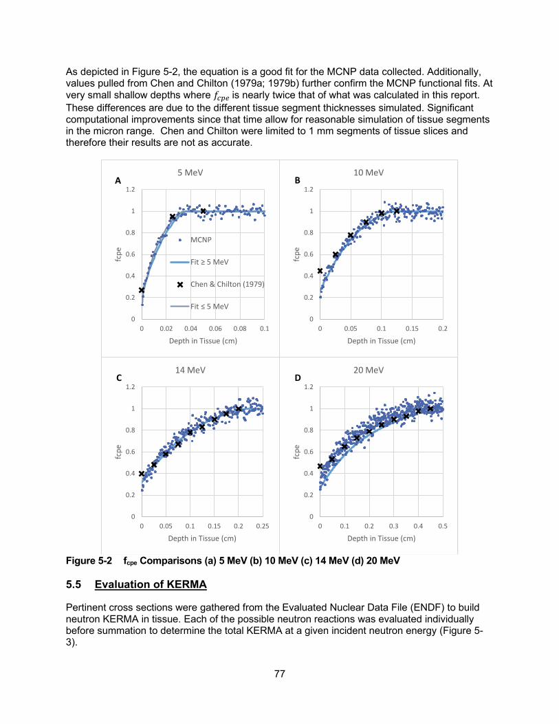
77

As depicted in Figure 5-2, the equation is a good fit for the MCNP data collected. Additionally, values pulled from Chen and Chilton (1979a; 1979b) further confirm the MCNP functional fits. At very small shallow depths where 𝑓𝑓𝑐𝑐𝑡𝑡𝑒𝑒 is nearly twice that of what was calculated in this report. These differences are due to the different tissue segment thicknesses simulated. Significant computational improvements since that time allow for reasonable simulation of tissue segments in the micron range. Chen and Chilton were limited to 1 mm segments of tissue slices and therefore their results are not as accurate.

Figure 5-2 fcpe Comparisons (a) 5 MeV (b) 10 MeV (c) 14 MeV (d) 20 MeV 5.5 Evaluation of KERMA

Pertinent cross sections were gathered from the Evaluated Nuclear Data File (ENDF) to build neutron KERMA in tissue. Each of the possible neutron reactions was evaluated individually before summation to determine the total KERMA at a given incident neutron energy (Figure 5-3).

0

0.2

0.4

0.6

0.8

1

1.2

0 0.02 0.04 0.06 0.08 0.1

fcpe

Depth in Tissue (cm)

5 MeV

MCNP

Fit ≥ 5 MeV

Chen & Chilton (1979)

Fit ≤ 5 MeV

A

0

0.2

0.4

0.6

0.8

1

1.2

0 0.05 0.1 0.15 0.2

fcpe

Depth in Tissue (cm)

10 MeVB

0

0.2

0.4

0.6

0.8

1

1.2

0 0.05 0.1 0.15 0.2 0.25

fcpe

Depth in Tissue (cm)

14 MeVC

0

0.2

0.4

0.6

0.8

1

1.2

0 0.1 0.2 0.3 0.4 0.5

fcpe

Depth in Tissue (cm)

20 MeVD

78

Figure 5-3 (a) Neutron KERMA versus Energy and Contribution per Element Compared

with ICRU 63; (b) Neutron KERMA versus Energy Detailed at the Higher Incident Neutron Energies, again Compared to ICRU 63 and to Liu and Chen (2008)

The evaluated data compare well with the ICRU values. However, there are variations in the higher MeV range primarily because of the modeling of threshold reactions in oxygen, nitrogen, and carbon. A previous study conducted by Liu and Chen (2008) evaluated the constituent KERMA extensively and reported a new set of values. Their results are compared in Figure 5-4 to the evaluated data from Anspach (2020) and ICRU recommendations.

1E-15

1E-14

1E-13

1E-12

1E-11

1E-10

1.00E-08 1.00E-06 1.00E-04 1.00E-02 1.00E+00

KERM

A (J

kg-1

cm2 )

Incident Neutron Energy (MeV)

Neutron KERMA

Hydrogen Carbon Nitrogen

Oxygen Total ICRU 63

0.00E+00

1.00E-11

2.00E-11

3.00E-11

4.00E-11

5.00E-11

6.00E-11

7.00E-11

8.00E-11

0.00 5.00 10.00 15.00 20.00

KERM

A (J

kg-1

cm2 )

Incident Neutron Energy (MeV)

Neutron KERMA

TOTAL ICRU 63 Liu & Chen (2008)

79

Figure 5-4 Threshold Reactions in each of the Four Constituents Accounted for in

KERMA as a Function of Incident Neutron Energy Using ICRU 63, “Nuclear Data for Neutron and Proton Radiotherapy and for Radiation Protection” for comparison, the recent difference for the reported KERMA values is determined over the entire energy range modeled as shown in Figure 5-5. Generally, there are three ranges with noticeable variations in their trends. This includes the energy ranges of 1x10-8 to 1x10-5 MeV, 1x10-5 to 1x10-2 MeV, and 1x10-2 to 20 MeV.

0

1E-11

2E-11

3E-11

4E-11

5E-11

0 5 10 15 20

KERM

A (J

kg-1

cm2 )

Incident Neutron Energy (MeV)

Hydrogen

Anspach

ICRU

Liu & Chen(2008)

A

0

1E-13

2E-13

3E-13

4E-13

5E-13

6E-13

7E-13

8E-13

9E-13

0 5 10 15 20

KERM

A (J

kg-1

cm2 )

Incident Neutron Energy (MeV)

NitrogenB

0

5E-13

1E-12

1.5E-12

2E-12

2.5E-12

3E-12

3.5E-12

4E-12

4.5E-12

0 5 10 15 20

KERM

A (J

kg-1

cm2 )

Incident Neutron Energy (MeV)

CarbonC

0

5E-12

1E-11

1.5E-11

2E-11

0 5 10 15 20

KERM

A (J

kg-1

cm2 )

Incident Neutron Energy (MeV)

OxygenD

80

Figure 5-5 Percent Difference Between Neutron Dose using ENDF Files versus ICRU 63 In the first energy range (Figure 5-6), the reaction that represents nearly the entire KERMA is the 14N(n,p)14C reaction with some fraction of the total KERMA due to radiative capture with hydrogen and other elemental constituents. Generally, the methods used here are in strong agreement (2-4 percent) with ICRU 63 in this energy range.

Figure 5-6 Reaction-Dependent KERMA in the Thermal Energy Range As energy increases (Figure 5-7), the probability for these reactions declines. In the energy range from 1x10-5 to 1x10-2 MeV, the probability for elastic scatter dramatically increases such

-10.00%

-8.00%

-6.00%

-4.00%

-2.00%

0.00%

2.00%

4.00%

6.00%

8.00%

10.00%

1.00E-08 1.00E-06 1.00E-04 1.00E-02 1.00E+00 1.00E+02

Devi

atio

n (%

)

Incident Neutron Energy (MeV)

% Difference ENDF vs ICRU

% Difference From ICRU

1E-16

1E-15

1E-14

1E-13

1E-12

1.00E-08 1.00E-07 1.00E-06 1.00E-05

KERM

A (J

kg-1

cm2 )

Energy (MeV)

Reaction Specific KERMA (0.01 eV - 10 eV)

N(n,p)C H(n,n)H ICRU 63 Total KERMA H(n,γ)H

81

that the dominant reaction mechanism is elastic scatter with hydrogen. Resultant data are still in good agreement with ICRU 63; however, the transition between these two reactions is a well-documented physical phenomenon such that any variation between methods will be represented systematically in the percent difference plot.

Figure 5-7 Reaction-Dependent KERMA in the Intermediate Energy Range Above 0.01 MeV (Figure 5-8), inelastic scatter and transfer reactions constitute a significant portion of total KERMA. Variation in this region is primarily due to the different cross-sectional data referenced. Published in 2000, the KERMA values of ICRU 63 (ICRU 2001) are based on the ENDF/B-V1.0 evaluated cross sectional data. In this report, cross section data from version VIII.0 (2018) is accessed. Figure 5-8 demonstrates the complexity of neutron KERMA in this energy range.

1E-15

1E-14

1E-13

1E-12

1.00E-05 1.00E-04 1.00E-03 1.00E-02

KERM

A (J

kg-1

cm2 )

Energy (MeV)

Reaction Specific KERMA (10 eV - 10 keV)

N(n,p)C H(n,n)H ICRU 63 Total KERMA

C(n,n)C N(n,n)N O(n,n)O

82

Figure 5-8 Reaction-Dependent KERMA in the Fast Energy Range 5.6 Neutron Dose from Radiative Capture

Whenever a nucleus enters an excited state, it has a high probability of emitting gamma rays to return to its ground state. In radiative capture, inelastic scatter, and transfer reactions, gamma rays are produced and will ultimately impart energy. However, unlike charged particles, they may travel significant distances before interacting with the medium or leaving it entirely. For small critical volumes, such as that where the shallow dose estimates are made, generated photons have a very small interaction probability. For larger volumes, such as the whole body, the interaction probability increases necessitating the determination of photon dose. This is especially important for thermal neutrons where the 1H(n,γ)2H capture reaction prevails. Concepts employed in internal dosimetry can be adopted to approximate photon dose. Since capture reactions within the human are a probabilistic occurrence, the production of photons is assumed to be randomly distributed throughout the entire body of the exposed. This concept is similar to a homogeneously distributed radionuclide that emits photons during radioactive decay. In this case, the number of photons produced per unit mass of a neutron-generated distributed gamma emitter is given by:

𝛾𝛾 �𝐷𝐷ℎ𝑆𝑆𝐷𝐷𝑆𝑆𝑙𝑙𝑠𝑠𝑘𝑘𝑔𝑔 � = Φ 𝑁𝑁𝑗𝑗 𝜎𝜎𝑠𝑠𝑗𝑗

where Φ is the neutron fluence, 𝑁𝑁𝑗𝑗 is the number of atoms per unit mass of a specific constituent, and 𝜎𝜎𝑠𝑠𝑗𝑗 is the cross section of that specific reaction leading to the production of photons. Photon production leads to dose by:

𝐷𝐷𝛾𝛾 = 𝛾𝛾 𝐹𝐹𝑎𝑎 𝐸𝐸𝛾𝛾 𝑘𝑘

1E-15

1E-14

1E-13

1E-12

1E-11

1E-10

1.00E-02 1.00E-01 1.00E+00 1.00E+01

KERM

A (J

kg-1

cm2 )

Energy (MeV)

Reaction Specific KERMA (10 keV - 20 MeV)

ICRU 63

Total KERMA

N(n,p)C

H(n,n)H

C(n,n)C

N(n,n)N

O(n,n)O

C Transfer

N Transfer

O Transfer

C Inelastic

N Inelastic

83

where 𝐹𝐹𝑎𝑎 is the absorbed fraction to the whole body from a photon of energy, 𝐸𝐸𝛾𝛾, and k is a unit conversion factor. Summing overall photon production reactions yields the total whole-body photon dose. ICRP 23, “Nuclear Data for Neutron and Proton Radiotherapy and for Radiation Protection” (ICRP 1975) reports a series of Monte-Carlo tests that determined the fraction of energy absorbed by a target organ from a photon of a specific energy emitted in a source organ. Figure 5-9 depicts the whole-body absorbed fraction, as a function of photon energy, from a homogeneously distributed whole-body source.

Figure 5-9 ICRP 23 Absorbed Fraction of Photon Energy Emitted from the Body and

Absorbed in the Body This process is separate from shallow neutron dosimetry where the assumption of charged particle equilibrium is not valid for fast neutrons. In this case, local energy deposition in small tissue volumes is the primary concern for neutron dose. Photons generated in these small critical volumes have a very low probability of interaction and are assumed to leave the critical target in its entirety. However, for whole body dosimetry where the tissue volume is many orders of magnitude larger than a 10-micron tissue segment, photon dose must be considered.

0.00%

10.00%

20.00%

30.00%

40.00%

50.00%

60.00%

70.00%

80.00%

90.00%

100.00%

0.01 0.1 1 10

Abso

rbed

Fra

ctio

n (%

)

Photon Energy (MeV)

ICRP 23 Absorbed Fraction

84

Figure 5-10 Absorbed Dose Due to Neutrons and Photons as a Function of Incident

Neutron Energy Below energies of about 1x10-3 MeV whole body radiation photon dose is nearly one order of magnitude larger than the neutron dose (Figure 5-10). This is primarily due to the relatively large hydrogen capture cross section. The effect of generated photons drops off beyond this energy until approximately 1 MeV where threshold inelastic and transfer reactions begin to occur. At this point the contribution to total dose from primarily inelastic photons begins to climb until it is approximately an order of magnitude less than the contribution from neutrons. From this, the method for whole body dosimetry is as follows:

𝐻𝐻(𝐸𝐸) = 𝐷𝐷𝛾𝛾(𝐸𝐸) ∙ 𝑤𝑤𝑅𝑅𝛾𝛾 + 𝐻𝐻𝑛𝑛(𝐸𝐸) where 𝐷𝐷𝛾𝛾(𝐸𝐸) is the absorbed dose from all photons produced from nuclear reactions associated with a specific neutron energy and 𝑤𝑤𝑅𝑅𝛾𝛾 is equal to unity (1), the radiation weighting factor for photons. The equivalent dose due to neutrons, 𝐻𝐻𝑛𝑛(𝐸𝐸) is described by the general neutron dosimetry model of NeutronDose, assigning fractional CPE a value of one, as CPE is assumed to be established.

1E-16

1E-15

1E-14

1E-13

1E-12

1E-11

1E-10

1.00E-08 1.00E-06 1.00E-04 1.00E-02 1.00E+00 1.00E+02

Gy (J

kg-1

cm2 )

Incident Neutron Energy (MeV)

Photon vs Neutron Dose

Photon Neutron Total

85

6 EYE DOSIMETRY MODEL

For VARSKIN+, a set of deterministic equations were developed from a vast array of probabilistic simulations to estimate radiation dose to the lens of the eye; the EyeDose module allows the user to quickly assess dose to the lens. EyeDose considers particle type (electrons and photons), particle energy, relative source distance from the eye, source emission rate, and the presence or absence of protective eyewear. The equations used in EyeDose were developed through Monte Carlo simulations of monoenergetic radioactive sources placed at varying distances from a stylized eye model, and they account for particle type, energy, source emission rate, and protective eyewear. The equations are valid for electron energies ranging from 100 keV to 11 MeV, photon energies ranging from 7 keV to 11 MeV, and distances from 0 to 20 meters. Additionally, sources emitting particles over an energy spectrum, such as beta sources, have been incorporated into this new dosimetry model. The source in EyeDose is modeled as an infinitely small, monoenergetic, isotropic point source of energy 𝐸𝐸. As seen in Figure 6-1, the source is located on the geometric axis of the eye and the distance between the surface of the eyeball and the source is labeled 𝑟𝑟. The target volume is taken to be the entire lens.

Figure 6-1 Eye Geometry Illustrating the Important Parameters used in the Deterministic

Dosimetry Model 6.1 Photon Dosimetry

The development of the photon model begins with the uncollided fluence equation, Φ0(𝑟𝑟) =

𝑆𝑆04𝜋𝜋𝑟𝑟2

,

[6.1]

86

and the fundamental equation for absorbed dose to a point in space at some distance r from an isotropic source of photons:

The lens, however, is a complex volume and not a single point. The probabilistic modeling software MCNP6 was used to determine dose to the human lens over a range of photon energies after passing through, and scattering in, air and the cornea. The resulting function for determining lens dose from photons of energy E emanating from an isotropic source at distance r, is

The parameters 𝐷𝐷, 𝑆𝑆, and 𝑚𝑚 describe the overall shape of the curve and 𝜇𝜇 is the mass attenuation coefficient in air. All four parameters are energy dependent. As this equation is a function of both distance 𝑟𝑟 and energy 𝐸𝐸, and 𝑟𝑟 is explicitly stated in Eq. [6.3], 𝐸𝐸 is implicit in the four parameters. The mass attenuation in air data were obtained from the NIST database of X-Ray Mass Attenuation Coefficients. Because this work focused on photon energies between 7 keV and 11 MeV, only a subset of the data was needed for the dosimetry model. An empirical function was derived from fitting over 720 rational functions to the data and it is valid for photon energies between 3 keV and 20 MeV. The mass attenuation coefficient for air can be described by

where 𝜌𝜌air = 1.205x10-3 g cm-3 is the density of dry air at sea level. Table 6-1 provides the coefficients of Eq. [6.4]. Table 6-1 Coefficients for the Mass Attenuation Coefficient for Photons in Air Empirical

Formula Subscript 𝑑𝑑 𝛼𝛼𝑠𝑠 𝛽𝛽𝑠𝑠 0 6.35455E-02 - 1 3.38929E-03 5.41880E-01 2 3.21001E-05 1.90162E-01 3 1.51457E-03 6.72185E-02 4 7.81438E-05 1.57391E-02 5 3.84722E-07 1.84372E-03 6 1.91620E-05 8.28629E-05

Eq. [6.3] was fitted against well over 2,500 data points. Once a fit was completed for a given energy, values for 𝐷𝐷, 𝑆𝑆, and 𝑚𝑚 were recorded and then plotted in Figure 6-2.

𝐷𝐷0(𝑟𝑟,𝐸𝐸) = 𝐸𝐸 Φ0 𝜇𝜇𝑒𝑒𝑛𝑛𝜌𝜌

𝐵𝐵 𝑠𝑠−𝜇𝜇𝑟𝑟. [6.2]

𝐷𝐷p(𝑟𝑟,𝐸𝐸) =exp(−𝜇𝜇𝑟𝑟)

𝐷𝐷𝑟𝑟2 + 𝑆𝑆𝑟𝑟 + 𝑚𝑚. [6.3]

�𝜇𝜇𝜌𝜌�air

=𝛼𝛼0 + ∑ 𝛼𝛼𝑠𝑠 ln𝑠𝑠 𝐸𝐸6

𝑠𝑠=1

1 +∑ 𝛽𝛽𝑠𝑠 ln𝑠𝑠 𝐸𝐸6𝑠𝑠=1

, [6.4]

87

Figure 6-2 Photon Dosimetry Shaping Parameters Plotted as a Function of Energy

All three parameters were fitted against more than 720 rational functions with the following results:

Table 6-2 gives the coefficients of Eqs. [6.5], [6.6], and [6.7].

𝐷𝐷 = exp �𝛼𝛼0 + ∑ 𝛼𝛼𝑠𝑠 ln𝑠𝑠 𝐸𝐸5

𝑠𝑠=1

1 +∑ 𝛽𝛽𝑠𝑠 ln𝑠𝑠 𝐸𝐸8𝑠𝑠=1

�, [6.5]

𝑆𝑆 = exp �𝛼𝛼0 + ∑ 𝛼𝛼𝑠𝑠 ln𝑠𝑠 𝐸𝐸9

𝑠𝑠=1

1 + ∑ 𝛽𝛽𝑠𝑠 ln𝑠𝑠 𝐸𝐸7𝑠𝑠=1

�,

[6.6]

and

𝑚𝑚 = exp �𝛼𝛼0 + ∑ 𝛼𝛼𝑠𝑠 ln𝑠𝑠 𝐸𝐸9

𝑠𝑠=1

1 +∑ 𝛽𝛽𝑠𝑠 ln𝑠𝑠 𝐸𝐸6𝑠𝑠=1

�. [6.7]

88

Table 6-2 Coefficients for the Shaping Parameters in the Photon Dosimetry Model 𝐷𝐷 𝑆𝑆 𝑚𝑚

𝛼𝛼0 9.44146E-01 1.01867E00 -1.18618E-01 𝛼𝛼1 -1.35506E00 -1.54109E00 -8.16699E-01 𝛼𝛼2 8.64682E-01 8.89146E-01 4.50464E-01 𝛼𝛼3 1.85547E-01 3.76454E-01 3.71586E-02 𝛼𝛼4 -1.01907E-01 -1.89178E-01 -2.01271E-01 𝛼𝛼5 -1.97434E-02 -1.46172E-02 -3.32457E-03 𝛼𝛼6 - 2.48789E-02 3.51748E-02 𝛼𝛼7 - -1.55929E-03 2.83451E-03 𝛼𝛼8 - -2.59795E-03 -2.16321E-03 𝛼𝛼9 - -3.09806E-04 -3.28384E-04 𝛽𝛽1 -5.72651E-01 -7.30645E-01 -3.74058E-01 𝛽𝛽2 2.02052E-01 -7.30645E-01 -3.74034E-02 𝛽𝛽3 2.28401E-01 3.75257E-01 3.71979E-01 𝛽𝛽4 -2.98566E-02 5.00708E-02 1.82485E-01 𝛽𝛽5 -3.57572E-02 5.00708E-02 1.82485E-01 𝛽𝛽6 -2.61996E-03 -1.17824E-02 1.33298E-03 𝛽𝛽7 1.110680E-03 -8.96010E-04 - 𝛽𝛽8 1.39853E-04 - -

Protective Glasses. The shielding used in the model is based on Spackman’s “classic” style eyewear (Spackman 2013). The posterior face of the lens is assumed to be normal to the eye’s geometric axis and located 1.05 cm in front of the cornea’s surface. Adding the lens thickness of 2 mm places its anterior face 1.25 cm from the cornea’s surface. To arrive at this distance, the head model used by Behrens et al. (2009) was inserted into the problem geometry and the lens was placed as close to the eye as possible without intersecting the head. The lenses were centered on the eye to simulate resting on the head model’s nose. The result is shown in Figure 6-3 with the eyewear placement at a fixed distance between the eye and the source of 1.25 cm.

89

Figure 6-3 Illustration of the Mathematical Parameters of the Shielded Model The concept of the buildup factor is extremely useful when estimating the dose after shielding has been introduced, 𝐷𝐷sh. The unshielded dose will be denoted by 𝐷𝐷unsh. Since the buildup factor is the ratio of total fluence to the primary fluence, total fluence can be expressed mathematically as:

Φ(𝐫𝐫) = 𝐵𝐵(𝐫𝐫)Φ0(𝐫𝐫), [6.8]

where Φ(𝐫𝐫) is the total fluence at point 𝐫𝐫, Φ0(𝐫𝐫) is the primary fluence at 𝐫𝐫, and the buildup factor is 𝐵𝐵(𝐫𝐫). Eq. [6.8] illustrates that the total fluence can be written as a function of the primary fluence. Combining this concept with the equation for dose written as 𝐷𝐷 =Φ𝐸𝐸 �𝜇𝜇𝑚𝑚𝑎𝑎

𝜌𝜌�, shows that the dose rate at a given point is related to the fluence at that point, and so

one may write:

𝐷𝐷sh(𝑟𝑟,𝐸𝐸) = 𝑓𝑓�𝐷𝐷unsh(𝑥𝑥,𝐸𝐸)�. [6.9]

Eq. [6.9] implies that knowledge of 𝐷𝐷unsh(𝑟𝑟,𝐸𝐸) is all that is needed to determine 𝐷𝐷sh(𝑟𝑟,𝐸𝐸). Indeed, when shielded and unshielded dose are plotted against each other, a nearly linear relationship is discovered. Figure 6-4 shows several examples. The mechanism in which photons interact with matter is highly dependent on the energy of the photon. Lower energy photons are more likely to undergo an absorption event than high-energy photons, and so shielding effectiveness tends to drop off with increasing photon energy. Photon buildup describes the process by which the number of scatter events increases as the number of absorption events decreases. This analysis considers this for higher energy photons, as several photons that would have otherwise missed are then redirected to the target volume. At some point, the shielding not only stops limiting the dose to the target volume but rather begins to increase the dose. In Figure 6-4, the dashed black line represents the case where shielding is no longer beneficial (that is, 𝐷𝐷sh(𝑟𝑟,𝐸𝐸) = 𝐷𝐷unsh(𝑟𝑟,𝐸𝐸)). For leaded eyewear, this occurs around 1 MeV. Photon energies greater than 1 MeV, such as the 3 MeV trend shown in Figure 6-4, tend

90

to deposit more energy into the target volume when shielding is present. This is not to say that leaded glasses should not be worn when 𝐸𝐸 > 1 MeV. If electrons are present, their contribution may be reduced by a greater factor if protection is worn, and so protective eyewear may offer a net decrease in dose. Section 6.2 discusses electron dosimetry.

Figure 6-4 Shielded Dose Plotted as a Function of Unshielded Dose Over 250,000 functions were tested against the data to find an empirical fit for Eq. [6.9]. The resulting equation that best fit the data was

𝐷𝐷sh = 𝐴𝐴𝐷𝐷unsh exp�𝑏𝑏𝐷𝐷𝑡𝑡𝑛𝑛𝑠𝑠ℎ + 𝑠𝑠�𝐷𝐷𝑡𝑡𝑛𝑛𝑠𝑠ℎ�, [6.10]

where 𝐴𝐴, 𝑏𝑏, and 𝑠𝑠 are energy dependent shaping parameters. In fact, 𝐴𝐴 can be viewed as an indicator of the level of protection provided by the leaded glasses. Protection is afforded when 𝐴𝐴 < 1. No protection is seen when 𝐴𝐴 ≈ 1 and 𝐷𝐷sh > 𝐷𝐷unsh when 𝐴𝐴 > 1. Figure 6-5, which shows the mass attenuation coefficient for lead, illustrates the K-edge at 0.088 MeV. The probability of an interaction occurring at this energy jumps dramatically, causing a break in the plot. It is because of this edge that the relationship between the shaping parameters must be split in two at 0.088 MeV. The jumps at the L-edges are much smaller and no split is necessary at these energies.

91

Figure 6-5 Mass Attenuation Coefficient for Lead The relationship between the three shaping parameters of Eq. [6.10] were determined from the analysis of 1,408 data points, giving the following:

𝐴𝐴 =

⎩⎪⎨

⎪⎧exp �𝛼𝛼0 + �𝛼𝛼𝑠𝑠 ln𝑠𝑠

𝐸𝐸1 + 𝐸𝐸

8

𝑠𝑠=1

� , 𝐸𝐸 > 0.088 MeV

exp �𝛼𝛼𝑠𝑠 + �𝛼𝛼𝑠𝑠𝐸𝐸𝑠𝑠6

𝑠𝑠=1

� , 𝐸𝐸 ≤ 0.088 MeV,

[6.11]

𝑏𝑏 =

⎩⎪⎨

⎪⎧ 𝛼𝛼0 + ∑ 𝛼𝛼𝑠𝑠𝐸𝐸𝑠𝑠5

𝑠𝑠=1

1 + ∑ 𝛽𝛽𝑠𝑠𝑠𝑠𝐸𝐸𝑠𝑠5

𝑠𝑠=1, 𝐸𝐸 > 0.088 MeV

𝛼𝛼0 + ln �1 + �𝐸𝐸 − 𝛼𝛼1𝛼𝛼2

�2� , 𝐸𝐸 ≤ 0.088 MeV,

[6.12]

and

𝑠𝑠 =

⎩⎪⎨

⎪⎧𝛼𝛼0 + ∑ 𝛼𝛼𝑠𝑠𝐸𝐸𝑠𝑠3

𝑠𝑠=1

1 +∑ 𝛽𝛽𝑠𝑠𝑠𝑠𝐸𝐸𝑠𝑠4

𝑠𝑠=1, 𝐸𝐸 > 0.088 MeV

𝛼𝛼𝑠𝑠 + �𝛼𝛼𝑠𝑠𝐸𝐸𝑠𝑠5

𝑠𝑠=1

, 𝐸𝐸 ≤ 0.088 MeV. [6.13]

Table 6-3 provides the vaues for coefficients 𝐴𝐴, 𝑏𝑏, and 𝑠𝑠. Photon energies from 7 keV to 11 MeV were tested. Energies below 50 keV yielded negligible dose and so can be taken to be 0. Eq. [6.11], [6.12], and [6.13] can be used for energies between 50 keV and 11 MeV. Distances from 1.25 cm to 20 m are valid.

92

Table 6-3 Coefficients for the Shaping Parameters of the Shielded Dose Equation 𝐸𝐸 > 0.088 MeV 𝐸𝐸 ≤ 0.088 MeV

𝐴𝐴 𝑏𝑏 𝑠𝑠 𝐴𝐴 𝑏𝑏 𝑠𝑠 𝛼𝛼0 3.13591E00 -1.29037E02 4.51223E-01 -1.94542E02 1.03174E00 -1.07048E02 𝛼𝛼1 2.15179E01 1.00768E02 -2.23710E01 1.21618E04 9.11942E-02 9.06704E03 𝛼𝛼2 6.43424E01 8.33501E02 -1.34607E00 -3.36015E05 7.08353E-04 -2.88345E05 𝛼𝛼3 1.09630E02 -2.39218E03 1.35608E02 5.09791E06 4.42100E06 𝛼𝛼4 1.15502E02 -1.90864E03 -4.41170E07 -3.30544E07 𝛼𝛼5 7.69484E01 1.51367E04 2.04591E08 9.69423E07 𝛼𝛼6 3.15687E01 -3.94653E08 𝛼𝛼7 7.28534E00 𝛼𝛼8 7.20570E-01 𝛽𝛽1 3.09273E03 -1.61930E00 𝛽𝛽2 -2.77860E03 -5.49709E01 𝛽𝛽3 -1.48815E03 3.33218E00 𝛽𝛽4 2.44611E02 7.32131E00 𝛽𝛽5 3.47614E02

6.2 Electron Dosimetry

Understanding the electron model in both shielded and unshielded circumstances first requires the analysis of the unshielded electron model in a vacuum. While the effects of air are too important to ignore, the final model is mathematically based on the initial conditions without air.

Because the bremsstrahlung plays a significant role in electron dosimetry, it must be considered. In fact, one may expect an electron point source dosimetry model to simply be the addition of the dose due to the electron source and the contribution from the bremsstrahlung source. An empirical model that fits the MCNP probabilistic data is:

The parameters 𝑚𝑚, 𝑏𝑏, 𝑠𝑠, 𝑑𝑑, 𝐷𝐷, 𝑆𝑆, and 𝑚𝑚 are all energy dependent shaping parameters. It was determined that adding 𝑠𝑠√𝑟𝑟 in the first term provided a better fit for lower energy electrons. The functions ℬ+ and ℬ− are modified hyperbolic tangent functions:

and

𝐷𝐷e(𝑟𝑟,𝐸𝐸) =ℬ+(𝐵𝐵, 𝑠𝑠)

𝑚𝑚𝑟𝑟2 + 𝑏𝑏𝑟𝑟 + 𝑠𝑠√𝑟𝑟 + 𝑑𝑑+

ℬ−(𝐵𝐵, 𝑠𝑠)𝐷𝐷𝑟𝑟2 + 𝑆𝑆𝑟𝑟 + 𝑚𝑚

. [6.14]

ℬ−(𝐵𝐵, 𝑠𝑠) ≡12

[1 − tanh 𝐵𝐵(𝑥𝑥 − 𝑠𝑠)] [6.15]

93

ℬ− and ℬ+ are sigmoid curves that vary between 0 and 1. Each ℬ is effectively a “continuous switch” that transitions between the two terms in Eq. [6.14]. The parameter 𝐵𝐵 controls how quickly ℬ changes from 0 to 1 and 𝑠𝑠 shifts the curve left and right. Figure 6-6 shows an example of both ℬ curves with 𝐵𝐵 set to 1 and 𝑠𝑠 set to 5.

Figure 6-6 The Switching Functions 𝓑𝓑+(q,s) and 𝓑𝓑-(q,s) with 𝒒𝒒 = 1 and 𝒔𝒔 = 5 Figure 6-7 shows the importance of bremsstrahlung for 0.65 MeV electrons. At distances less than 0.3 cm, bremsstrahlung contributes 100 percent of the total dose. Electrons begin directly contributing to the total dose when 𝑟𝑟 ≈ 0.3 cm.

Figure 6-7 Total Dose to the Lens from 0.65 MeV Electrons with the Bremsstrahlung

KERMA Called Out

ℬ+(𝐵𝐵, 𝑠𝑠) ≡12

[1 + tanh 𝐵𝐵(𝑥𝑥 − 𝑠𝑠)]. [6-16]

94

Figure 6-8 Total Dose to the Lens from 0.65 MeV Electrons on Log-Log Axes This phenomenon results from the shape of the eye itself. Consider Figure 6-9, which shows two cases. In the first case, the electron source is very close to the eye. The route between the source and the lens with the least amount of tissue is normally incident and shown by the black arrow. Some electrons may not have enough energy to penetrate through this tissue, leaving bremsstrahlung as the only contributor to the total dose. In the second case, the electron source has been pulled back some distance. The normal route is still too thick for lower energy electrons to penetrate. However, consider the dashed purple line emanating from the source to the top of the cornea. Electrons that are incident in this region have a chance to be deflected along the second arrow. Due to the eyeball’s curvature, this new path requires the electron to travel through less tissue before reaching the target volume. This new path opens at around 𝑟𝑟 = 0.3 cm. The electron rays radiating from the source can be considered parallel at about 10 cm, at which point both the bremsstrahlung and direct contribution obey the inverse square law.

95

Figure 6-9 Schematic Representation of how Curved Surfaces Result in Dose from

scattered Electrons A 3rd term seems to be needed in Eq. [6.14] to account for the scattered electron contribution. It turns out, however, that the first term can describe both the bremsstrahlung and scattered electron contributions. This allows the combination of the bremsstrahlung and scattered contributions into a single term, written as:

To illustrate the effectiveness of Eq. [6.17], consider the plots for 1 and 3 MeV electrons seen in Figure 6-10 and Figure 6-11. In both cases the bremsstrahlung contribution is negligible. The 1 MeV electrons have enough energy to penetrate directly to the lens at all distances. The reduced penetration depth for 𝑟𝑟 > 0.3 cm provides a pathway for the scattered dose, resulting in the odd shape seen in Figure 6-10. The higher energy 3 MeV electrons can easily penetrate to the target volume and the direct electron contribution dominates the shape seen in Figure 6-11, though scattered electrons are still a considerable portion of the total dose.

𝐷𝐷e,vac(𝑟𝑟,𝐸𝐸) =ℬ−(𝐵𝐵, 𝑠𝑠)

𝑚𝑚𝑟𝑟2 + 𝑏𝑏𝑟𝑟 + 𝑠𝑠√𝑟𝑟 + 𝑑𝑑+

ℬ+(𝐵𝐵, 𝑠𝑠)𝐷𝐷𝑟𝑟2 + 𝑆𝑆𝑟𝑟 + 𝑚𝑚

. [6.17]

96

Figure 6-10 Lens Dose from 1 MeV Electrons on both Linear-Log and Log-Log Axes

97

Figure 6-11 Lens Dose from 3 MeV Electrons on both Linear-Log and Log-Log Axes

Additional parameters to modify Eq. [6.3] are needed to account for energy degradation in air. Simplicity would suggest the following:

𝐷𝐷air = 𝑓𝑓�𝐷𝐷vac,𝜇𝜇e(𝑟𝑟,𝐸𝐸)�, [6.18]

98

where 𝜇𝜇e(𝑟𝑟,𝐸𝐸) is a function that accurately describes the impact that air has on electron dosimetry. Generally, one could write 𝐷𝐷air = 𝐷𝐷vac exp(−ℎ𝑟𝑟), where ℎ behaves similarly to 𝜇𝜇 for photons. This formulation fails for purposes of this analysis, though, for three reasons. (1) The analysis concerns distances in air up to 10 m. (2) The size and shape of the target volume play a significant role in electron dosimetry. (3) Bremsstrahlung generated in air is a key component of electron dose.

Rather, while traversing through space, the electron fluence undergoes dramatic transformations that are not adequately described by simple exponential decay. An empirical expression accounting for the effects of air was derived:

Figure 6-12 shows the absorbed dose from a point source in air and in a vacuum. There is good agreement between the two when the source is less than about 1 cm from the eye, but subtle differences begin to emerge between 1 cm and 10 cm. The two curves clearly diverge beyond 10 cm, and careful inspection of the air model indicates a bend at about 100 cm. It was discovered that ℬ− accurately describes the initial deviation between the vacuum and air data. The bend can be modeled by the third term in Eq. [6.19]. Equation [6.19] is further broken down in Figure 6-13. The data collected through MCNP are shown as blue dots. Each term in Eq. [6.19] is individually plotted. The dosimetry model, shown as a solid red line, is the summation of these three terms.

Figure 6-12 Comparison of the Dose for 0.65 MeV Electron Point Sources in Air and in

Vacuum

𝐷𝐷air =ℬ−(𝐵𝐵, 𝑠𝑠)

𝑚𝑚𝑟𝑟2 + 𝑏𝑏𝑟𝑟 + 𝑠𝑠√𝑟𝑟 + 𝑑𝑑+ℬ+(𝐵𝐵, 𝑠𝑠) ℬ−(𝑚𝑚, 𝑙𝑙)𝐷𝐷𝑟𝑟2 + 𝑆𝑆𝑟𝑟 + 𝑚𝑚

+𝑘𝑘 ℬ+(1000, 𝑧𝑧)

(1 + 𝑟𝑟)𝑗𝑗 . [6.19]

99

Figure 6-13 Component Breakdown of the Electron Dosimetry Model Each term in Eq. [6.19] is a continuous differential function for 𝑟𝑟 > 0. This implies that 𝐷𝐷air must be continuous and differential as well. Equation [6.19] is a very complicated model containing 14 parameters in total. This complexity prohibits the establishment of an equation for each parameter. Incorporating shielding for electrons requires a slight modification of Eq. [6.19] and recalculation of each of the shaping parameters. Similarly, the shielded electron dose model is:

6.3 Continuous Radiation Sources

Many commonly found radioactive sources are beta emitters. These emitted beta particles are essentially high-speed electrons born from nuclear decay. Unlike gamma rays, which are radiated at discrete and predictable energies, betas are released in a continuous energy spectrum. In addition to continuous beta spectra, continuous photon spectra may be encountered, especially in medical and industrial settings. Equation [6.19] was developed for monoenergetic sources and is not immediately applicable to continuous sources of radiation. However, Eq. [6.19] can still be used for these sources with the following procedure. Assume 𝑌𝑌(𝐸𝐸) describes the continuous energy spectrum for a given source and define:

𝐸𝐸(𝐸𝐸) ≡𝑌𝑌(𝐸𝐸)

∫ 𝑌𝑌(𝐸𝐸)𝑑𝑑𝐸𝐸 [6.21]

to represent the number of particles emitted per unit energy per disintegration. 𝐸𝐸(𝐸𝐸) is fundamentally a normalized 𝑌𝑌(𝐸𝐸) since 𝐸𝐸(𝐸𝐸) = 𝑌𝑌(𝐸𝐸) if and only if ∫ 𝑌𝑌(𝐸𝐸)𝑑𝑑𝐸𝐸 = 1. The product

𝐷𝐷sh = �ℬ−(𝐵𝐵, 𝑠𝑠)

𝑚𝑚𝑟𝑟2 + 𝑏𝑏𝑟𝑟 + 𝑠𝑠√𝑟𝑟 + 𝑑𝑑+ℬ+(𝐵𝐵, 𝑠𝑠) ℬ−(𝑚𝑚,𝑙𝑙)𝐷𝐷𝑟𝑟2 + 𝑆𝑆𝑟𝑟 + 𝑚𝑚

+𝑘𝑘 ℬ+(1000, 𝑧𝑧)

(1 + 𝑟𝑟)𝑗𝑗 � [ℬ−(𝐺𝐺, 0)]. [6.20]

100

𝐷𝐷(𝑟𝑟,𝐸𝐸) ∙ 𝐸𝐸(𝐸𝐸) [6.22]

is the lens dose per unit energy deposited by a particle of energy 𝐸𝐸 at distance 𝑟𝑟. The total lens dose is found by integrating Eq. [6.22]:

𝐷𝐷total = �𝐷𝐷(𝐸𝐸) ∙ 𝐸𝐸(𝐸𝐸)𝑑𝑑𝐸𝐸𝐸𝐸

. [6.23]

In the presence of discrete energy particles (such as Auger electrons, characteristic x-rays or gamma rays) and continuous energy spectra (such as beta radiation or x-ray machines), Eq. [6.23] can be generalized to

�̇�𝐷total = � 𝐴𝐴𝑠𝑠𝐷𝐷p(𝐸𝐸)discretephotons

+ � 𝐴𝐴𝑠𝑠 �𝐷𝐷p(𝐸𝐸) ∙ 𝐸𝐸𝑠𝑠(𝐸𝐸)𝑑𝑑𝐸𝐸𝐸𝐸continuous

photons

+ � 𝐴𝐴𝑠𝑠𝐷𝐷e(𝐸𝐸)discreteelectrons

+ � 𝐴𝐴𝑠𝑠 �𝐷𝐷e(𝐸𝐸) ∙ 𝐸𝐸𝑠𝑠(𝐸𝐸)𝑑𝑑𝐸𝐸𝐸𝐸continuous

electrons

.

[6.24]

In Eq. [6.24], each 𝐴𝐴𝑠𝑠 is the emission rate for the 𝑑𝑑th particle in the group. Because each 𝐴𝐴𝑠𝑠 is an emission rate, Eq. [6.24] represents the total lens dose rate.

6.4 Verification and Validation

Photons. To illustrate how Eq. [6.3] fits the data, consider its weighted fit to 1 MeV photons, shown in Figure 6-14 and Figure 6-15. The overall shape of the function matches the data quite well, and the mean percent error (MPE) is bounded between ±0.8 percent, where the MPE is a scale-independent and unbiased measure of error between the data and the predictive model. The inverse square law predicts the photon density with respect to distance from the point source’s spatial location. Points near the source will have a higher photon density than points farther from the source. The photon density is directly proportional to the number of interactions occurring in the volume, and so the number of interactions per history is expected to increase as the source is placed successively closer to the target volume. Thus, for the same number of MCNP histories, photons closer to the target volume will be associated with higher levels of certainty, and hence, higher weights. Figure 6-15 illustrates this where the MPE for 𝑟𝑟 < 1 cm is less than the MPE for larger 𝑟𝑟. Figure 6-16 provides a separate indication that the model adequately represents the data over the entire range of distances.

101

Figure 6-14 An Empirical Function Fitted Against the Absorbed Dose to the Lens for 1 MeV

Photons in Air

Figure 6-15 A Weighted MPE Residual Plot for the Photon Dosimetry Model Empirical Fit

102

Figure 6-16 The Comparison Plot for a 1 MeV Photon Point Source To illustrate how well Eq. [6.4] fits the data, consider Figure 6-17 and Figure 6-18. Figure 6-17 shows the empirical model overlaid on the mass attenuation data. The residual plot shown in Figure 6-18 indicates that the MPE between the function and the data is bounded by ±0.08 percent and shows no predictable pattern, indicating an excellent fit.

Figure 6-17 An Empirical Function Fitted Against the Mass Attenuation Coefficient for

Photons in Air

103

Figure 6-18 The MPE Residual Plot for the Empirical Fit of the Mass Attenuation Coefficient

in Air To demonstrate the model’s accuracy, 2,713 data points of varying energies and distances along the geometric axis were collected by simulation in MCNP and compared to the lens dose model. Figure 6-10 shows the comparison plot resulting from these estimations. This plot shows only very minor deviations between the observed and predicted values.

Figure 6-19 Comparison Plot of Photon Model and 2,713 Data Points

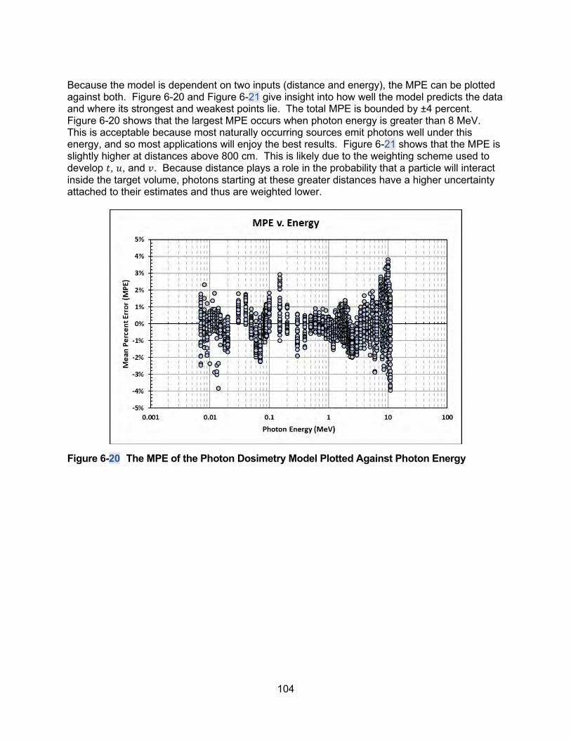
104

Because the model is dependent on two inputs (distance and energy), the MPE can be plotted against both. Figure 6-20 and Figure 6-21 give insight into how well the model predicts the data and where its strongest and weakest points lie. The total MPE is bounded by ±4 percent. Figure 6-20 shows that the largest MPE occurs when photon energy is greater than 8 MeV. This is acceptable because most naturally occurring sources emit photons well under this energy, and so most applications will enjoy the best results. Figure 6-21 shows that the MPE is slightly higher at distances above 800 cm. This is likely due to the weighting scheme used to develop 𝐷𝐷, 𝑆𝑆, and 𝑚𝑚. Because distance plays a role in the probability that a particle will interact inside the target volume, photons starting at these greater distances have a higher uncertainty attached to their estimates and thus are weighted lower.

Figure 6-20 The MPE of the Photon Dosimetry Model Plotted Against Photon Energy

105

Figure 6-21 The MPE of the Photon Dosimetry Model Plotted Against Distance A goodness of fit analysis was carried out as described in Section 6.1. The worst fits appear at 50 keV and 1.25 cm. The MPE is bounded by ±3 percent for all other energies except 60 keV and 11 MeV, which have lower bounds of 5 percent. The comparison plot and residual plots are shown in Figure 6-22, Figure 6-13, and Figure 6-14.

Figure 6-22 Plot of the MPE versus Energy for the Shielded Dose Model

106

Figure 6-23 Plot of the MPE versus Distance for the Shielded Dose Model

Figure 6-24 Comparison Plot for the Shielded Dose Model

Electrons. Figure 6-25 and Figure 6-26 show the comparison plot between 1,652 data points collected via MCNP simulations and the electron dosimetry model. It is apparent that the model fits very well when the observed dose is greater than about 1x10-6 pGy/electron. Some doses below this threshold begin to deviate from the line 𝐺𝐺 = 𝑥𝑥. These deviations are to be expected when air is considered, as air has a significant impact on electron behavior. The farther an

107

electron must travel through air to reach its target, the wider the resulting dose distribution in the target volume.

Figure 6-25 Comparison Plot for Unshielded Electrons in Air on Linear Axes

Figure 6-26 Comparison Plot for Unshielded Electrons in Air on Log-Log Axes

Parameters for Eq. [6.20] are given for energies above 80 keV and below 11 MeV. Doses at lower energies are negligible and can be taken to be 0. Figure 6-27 and Figure 6-28 provide the

108

comparison plots for the shielded electron model on linear and log-log axes. Both plots show excellent agreement. A few points near the bottom in Figure 6-28 appear to deviate significantly from the line 𝐺𝐺 = 𝑥𝑥. These data are not an issue, however, because they are extremely low values of dose and may be considered negligible in most scenarios.

Figure 6-27 Comparison Plot on Linear Axes for Electrons Shielded with Protective Leaded Eyewear

Figure 6-28 Comparison Plot on Log-Log Axes for Electrons Shielded with Protective Leaded Eyewear

Figure 6-29 illustrates the validity of Eq. [6.24]. Three beta sources (P-32, Y-90, and Sr-90) and a 120 kVp X-ray source were modeled in MCNP as continuous energy spectrum point sources.

109

In each example, a source emission rate of 4x1010 emissions per second is assumed. Data collected in MCNP are shown as points while the dosimetry model is shown as a solid line. Error bars represent the 1σ confidence interval. All four examples show excellent agreement, with the largest discrepancies occurring when a beta source was placed more than 100 cm from the eye. Even so, the difference between the observed value and the predicted value is very small.

Figure 6-29 Plot of the Lens Dose Rate for Selected Continuous Radiation Point Sources Alternatively, the SkinDose module can be made to loosely simulate the lens. Figure 6-30 provides a cross-sectional view of how SkinDose can be used to simulate the eye. A cylinder, shown in yellow, simulates the lens. It is located 0.321 cm below the tissue surface and is 0.43 cm thick. The circular surface area of one face is 1 cm². The blue region represents air, and the peach region represents tissue. This representation does not consider the curvature of the eye, the curvature of the lens, and the varying densities of the tissues of the eye.

Figure 6-30 Schematic used by SkinDose to Simulate the Lens Several comparisons were made between this setup in SkinDose, and the models developed in this project. Figure 6-31 shows the results of these comparisons. Results are fairly close in

110

most scenarios, but a few stand out, particularly with a low energy electron source. For example, the dose from 0.65 MeV electrons is severely overestimated at 0 cm and 1 cm but underestimated by a factor of about 10 at 10 cm. Additionally, negative electron contributions were recorded for Co-60 at all distances. These inconsistencies are likely artifacts of how SkinDose performs volume averaging. Low energy electrons are unable to penetrate deep enough to reach the lens and so their scores are not properly calculated. Photons showed better agreement than electrons, but discrepancies were still noted. SkinDose was unable to calculate any dose closer than 5 cm for Co-60. Also, the photon dose due to Holmium (Ho)-166 was considerably underestimated in all cases.

Figure 6-31 Comparison of Calculations Between SkinDose and this Model

111

6.5 Limitations (Off-Axis Sensitivity Analysis)

A mathematical model of a physical event is only as good as its most uncertain parameter. The model presented here essentially assumes the eyeball being irradiated is staring directly at the source for the entire exposure, an assumption that does not hold up in all circumstances. It is therefore desirable to understand how the spatial location of the source relative to the eye can affect dose to the lens. Consider a source that is located off the eye’s geometric axis (Figure 6-32). This off-axis source is located a distance 𝑟𝑟 from the eye and makes an angle 𝜃𝜃 from the geometric axis.

Figure 6-32 Parameter Definitions for an Off-Axis Source. The following is a rudimentary analysis of the model’s sensitivity to source placement. Let 𝐷𝐷(𝑟𝑟,𝜃𝜃) denote the lens dose for a source located at the point (𝑟𝑟,𝜃𝜃) as seen in Figure 6-32. 𝐷𝐷(𝑟𝑟,𝜃𝜃) was collected from MCNP simulations for 𝑟𝑟 = 0.1, 1, and 10 cm and 𝜃𝜃 ranging from 0° to 90° in 10° increments. Photon energies considered were 10 keV, 1 MeV, and 10 MeV. Electron energies were 60 keV, 1 MeV, and 3 MeV. A total of 180 simulations were run (90 for each particle type). The head phantom was not modeled. In each simulation, the ratio between the off-axis dose 𝐷𝐷(𝑟𝑟,𝜃𝜃) and the on-axis dose 𝐷𝐷(𝑟𝑟, 0°) was recorded and plotted. Figure 6-33 and Figure 6-34 show the results. The data clearly indicate that the lens dose depends on the source’s spatial location. Furthermore, this dependency is also reliant on the source’s energy. The data also indicate that the difference between the on-axis and off-axis dose might be within 20 percent provided that 𝜃𝜃 < 20°.

112

Figure 6-33 𝑫𝑫(𝒓𝒓,𝜽𝜽) for Photons with 𝒓𝒓 = 0.1, 1, and 10 cm and 𝜽𝜽 Ranging from 0° to 90° in

10° Increments

113

Figure 6-34 𝑫𝑫(𝒓𝒓,𝜽𝜽) for Electrons with 𝒓𝒓 = 0.1, 1, and 10 cm and 𝜽𝜽 Ranging from 0° to 90° in

10° Increments

115

7 REFERENCES

Anderson, M.E. and R.A. Neff. Neutron energy spectra of different size 239Pu-Be(α,n) sources. Nucl. Instrum. Methods. 99:231-235. 1972. Anspach, L.J. Development of a fundamental depth-dependent neutron dosimetry model. Master’s Thesis. Oregon State University. Corvallis, OR: 2020. Anspach, L.J. and D.M. Hamby, D.M. Performance of the VARSKIN 5 (v5.3) Electron Dosimetry Model. Radiation Protection Dosimetry. DOI:10.1093/rpd/ncx302. December 2017. Attix, F.H. Introduction to Radiological Physics and Radiation Dosimetry. John Wiley & Sons. New York, NY. 1986. Berger, M.J. “Distribution of Absorbed Dose around Point Sources of Electrons and Beta Particles in Water and Other Media.” Medical Internal Radiation Dose Committee, Pamphlet No. 7. Journal of Nuclear Medicine. Vol. 12, Supplement No. 5. pp. 5–22. 1971. Behrens, R., G. Dietze, and Z. Maria. "Dose conversion coefficients for electron exposure of the human eye lens." Physics in Medicine and Biology. 54 (13): 4069-4087. 2009. Chen, S.Y. and A.B. Chilton. Depth-Dose Relationship near the Skin Resulting from Parallel Beams of Fast Neutrons. Radiation Research. 77(1): 21-33. 1979a. Chen, S.Y. and A.B. Chilton. Calculation of Fast Neutron Depth-Dose in the ICRU Standard Tissue Phantom and the Derivation of Neutron Fluence-to-Dose-Index Conversion Factors. Radiation Research. 78(3): 335-370. 1979b. Cross, W.G., N.O. Freedman, and P.Y. Wong. “Tables of Beta-Ray Dose Distributions in Water.” AECL 10521, CA9200298. Chalk River Laboratories, Dosimetric Research Branch. Chalk River. Ontario, Canada. 1992. Dubeau, J., S.S. Hakmana Witharana, J. Sun, B.E. Heinmiller, and W.J. Chase. A Comparison of Beta Skin Doses Calculated with VARSKIN 5.3 and MCNP5. Radiation Protection Dosimetry. DOI:10.1093/rpd/ncy108; July 2018. Electric Power Research Institute (EPRI). Implementing the EPRI effective dose equivalent (EDE) methodology for discrete radioactive particles on the skin. Report No. 1002823. 2004. International Commission on Radiation Units and Measurements. “Tissue Substitutes in Radiation Dosimetry and Measurement.” ICRU Report 44. Bethesda, MD: International Commission on Radiation Units and Measurements. 1989. International Commission on Radiation Units and Measurements. “Nuclear Data for Neutron and Proton Radiotherapy and for Radiation Protection.” ICRU Report 63. Bethesda, MD: International Commission on Radiation Units and Measurements. 2001. International Commission on Radiological Protection. “Reference Man: Anatomical, Physiological, and Metabolic Characteristics.” Publication 23. Oxford, England: Pergamon

116

Press. 1975. International Commission on Radiological Protection. “Radionuclide Transformations.” Publication 38. Oxford, England: Pergamon Press. 1983. International Commission on Radiological Protection. “The Biological Basis for Dose Limitation in the Skin.” Publication 59. Oxford, England: Pergamon Press. 1991. International Commission on Radiation Protection. “Nuclear Decay Data for Dosimetric Calculations.” Publication 107. Ann. ICRP 38 (3). 2008 Johns, H.E. and J.R. Cunningham. The Physics of Radiology. 4th Edition. Springfield, IL: Charles C. Thomas. 1983. Kawrakow, I. and D.W. Rogers. The EGSnrc code system: Monte Carlo simulation of electron and photon transport. Technical Report PIRS-701. Ottawa, Canada: National Research Council of Canada. 2000. Klumpp, J., L. Bertelli, S. Dumit, M. Gadd, D. Poudel, and T.L. Waters. Response to a Skin Puncture Contamination with 238Pu at Los Alamos National Laboratory. Health Physics. 119(6): 704-714; 2020. Liu, Z. and J. Chen. New Calculations of Neutron Kerma Coefficients and Dose Equivalent. Journal of Radiological Protection, 28, 185-193. 2008. Ljungberg, M., S.E. Strand, and M.A. King. Monte Carlo Calculations in Nuclear Medicine, Second Edition. CRC Press. Chapter 10:175–195; 2012. Lorch, E.A. Neutron spectra of 241Am/B, 241Am/Be, 241Am/Fe, 242Cm, 239Pu/13C and 252Cf isotopic neutron source. J. Appl. Radiat. Isot. 24:585-591. 1973. Los Alamos National Laboratory, X-5 Monte Carlo Team. “MCNP—A General Monte Carlo N-Particle Transport Code, Version 5. LA-CP-03-0245. Los Alamos, NM: LANL. 2003. Mangini, C.D. and D.M. Hamby. “Scaling Parameters for Hot-Particle Beta Dosimetry”. Radiation Protection Dosimetry. 172(4): 356-366; 2016. Mangini, C.D. “Beta-particle backscatter factors and energy-absorption scaling factors for use with dose-point kernels.” Doctoral Dissertation. Oregon State University. December 2012. McDaniel, N.S. and D.M. Hamby. The Efficacy of VARSKIN 5.3 for Eye Dosimetry. VARSKIN Technical Session. Annual Domestic RAMP User’s Meeting. Bethesda, MD; October 2017. National Council on Radiological Protection & Measurement (NCRP). Development of a biokinetic model for radionuclide-contaminated wounds and procedures for their assessment, dosimetry and therapy. Report No. 156. Bethesda, MD; 2007. Piechowski, J. and Y. Chaptinel. Evaluation of local dose for a contaminated wound. Radioprotection. 39(3):355-366; 2004 (in French).

117

Radiation Dosimetry Calculations for ICRP and MIRD.” CCC–701. Oak Ridge, TN: RSICC. 1995. Rogers, D.W.O. Fifty years of Monte Carlo simulations for medical physics. Physics in Medicine and Biology. 51: R287-R301; 2006. Sherbini, S., J. DeCicco, A.T. Gray, and R. Struckmeyer. “Verification of the Varskin Beta Skin Dose Calculation Computer Code,” Health Physics. 94: 527–538; 2008. Shultis, J.K. and Faw, R.E. Radiation Shielding. American Nuclear Society. ISBN 0-89448-4567. La Grange Park, IL. 2000. Spackman, D.A. "Design and Analysis of Radiation Shielding Eyewear." Master’s Thesis. Oregon State University. Corvallis, OR: 2013. Spencer, L. V. Theory of electron Penetration. Physical Review. 98: 1597-1615; 1955. Spencer, L. V. Energy Dissipation by Fast Electrons. National Bureau of Standards Monograph 1; 1959. Toohey, R.E., L. Bertelli, S.L. Sugarman, A.L. Wiley, and D.M. Christensen. Dose coefficients for intakes of radionuclides via contaminated wounds. Oak Ridge Institute for Science and Education. DOE Contract No. DE-AC05-06OR23100. Oak Ridge, TN; Ver. 2, August 2014. U.S. Nuclear Regulatory Commission. Traub, R.J., W.D. Reece, R.I. Scherpelz, and L.A. Sigalla. “Dose Calculation for Contamination of the Skin Using the Computer Code VARSKIN.” NUREG/CR–4418. Washington, DC: NRC. 1987. U.S. Nuclear Regulatory Commission. Reece, W.D., S.D. Miller, and J.S. Durham. “SADDE (Scaled Absorbed Dose Distribution Evaluator), A Code to Generate Input for VARSKIN.” NUREG/CR–5276. Washington, DC: NRC. 1989. U.S. Nuclear Regulatory Commission. Durham, J.S. “VARSKIN Mod 2 and SADDE Mod 2: Computer Codes for Assessing Skin Dose from Skin Contamination.” NUREG/CR-5873, PNL-7913. Washington, DC: NRC. 1992. U.S. Nuclear Regulatory Commission. Durham, J.S. “VARSKIN 3: A Computer Code for Assessing Skin Dose from Skin Contamination.” NUREG/CR-6918. Washington, DC: U.S. Nuclear Regulatory Commission. 2006. U.S. Nuclear Regulatory Commission. Hamby, D.M., Lodwick, C.J., Palmer, T.S., Reese, S.R., Higley, K.A. “VARSKIN 4: A Computer Code for Skin Contamination Dosimetry.” NUREG/CR-6918, Rev 1. Washington, DC: U.S. Nuclear Regulatory Commission. 2011. U.S. Nuclear Regulatory Commission. Hamby, D.M., Mangini, C.D., Caffrey, J.A., Tang, M. “VARSKIN 5: A Computer Code for Skin Contamination Dosimetry.” NUREG/CR-6918, Rev 2. Washington, DC: U.S. Nuclear Regulatory Commission. 2014. U.S. Nuclear Regulatory Commission. Hamby, D.M., Mangini, C.D. “VARSKIN 6: A Computer Code for Skin Contamination Dosimetry.” NUREG/CR-6918, Rev 3. Washington, DC: U.S. Nuclear Regulatory Commission. 2018.

118

U.S. Nuclear Regulatory Commission. News Release No. 02-039. April 2, 2002. https://www.nrc.gov/docs/ML0209/ML020990362.pdf Last accessed January 2021. Walsh, R.L. Spin-dependent calculations of fission neutron spectra and fission spectrum integrals for six fissioning systems. Nuc. Sci. Eng. 102:119-133. 1989.

A-1

APPENDIX A EXAMPLES AND SOLUTIONS USING VARSKIN+

Examples Using the SkinDose Module This appendix describes four different practical applications of SkinDose using an example/solution format. Each example describes a situation followed by a solution that involves the use of SkinDose to estimate shallow dose at 7 mg/cm2 and dose at a depth of 1,000 mg/cm2. The purpose of these examples is to lead a new user of SkinDose through several calculations that highlight many of its features. Because SkinDose is a flexible tool, there are always several ways to calculate the dose for a given example. The solutions presented here reflect the recommendations that are provided throughout the user’s manual. With some experience, most SkinDose users will not need to perform all the steps described in the solution in an actual situation. It is suggested that the user complete all four examples in the order in which they are presented to become familiar with SkinDose. It is important to note that, even though SkinDose is used to calculate dose at depths other than 7 mg/cm2, these values do not ensure compliance with the requirements of Title 10 of the Code of Federal Regulations (10 CFR) Part 20, “Standards for protection against radiation”. The examples here simply change the tissue depth from 7 mg/cm2 to some different value without changing other pertinent parameters of the dose-averaging calculation. Note that when, in the following scenarios, the depth is changed from 7 mg/cm2 to 1,000 mg/cm2, for example, the purpose is not necessarily to calculate deep dose equivalent, but simply to demonstrate the utility of the code for estimating energy absorption at various depths in tissue. Example 1: Radiopharmaceutical Technologist in Nuclear Medicine At a research hospital, a doctor prescribes a 5-milliliter (mL) administration from a stock solution containing 370 kiloBequerels per milliliter (kBq/mL) of rhenium (Re)-186 for a clinical research study at 1 p.m. that day. Around 12:30 p.m., a lab technologist loads the dose under the hood. Subsequently, a fellow employee bumps into her, and the needle slips out of its container. The entire 5 mL of the solution is spilled on the arm of her cloth lab coat in a circular shape with an area of approximately 50 square centimeters (cm2). She is unaware of the accident and continues with her work until the end of the day. Around 5 p.m., a routine survey discovers the contamination. Solution 1: Radiopharmaceutical Technologist in Nuclear Medicine The point source geometry is suggested as a starting point to estimate the magnitude of the dose and to collect some other useful information. Run SkinDose and select the “Nuclide List” button. If 186Re does not appear in the radionuclide library (in the “Available in Database” window), add Re-186 by selecting the database radio button for International Commission on Radiation Protection (ICRP) Publication 107, “Nuclear Decay Data for Dosimetric Calculations”, issued 2008, confirming the effective Z of 7.42, and double-click on “Re-186”. When “Re-186 (7.42, 107)” appears in the “Selected for Analysis” box, return to the SkinDose window. Confirm the Dose Depth of 7 mg/cm2. Enter the Exposure Time as 4.5 followed by the Tab key and change the time unit to hours using the dropdown menu. Confirm that the dose-averaging area is 10 cm2 and that there is zero airgap. Also, confirm that the Volume Averaging and Backscatter disable radio buttons are NOT selected and that the Dose Equivalent Units are in “mSv”.

A-2

Because the point source geometry is being used, it is necessary to calculate the source strength by multiplying the concentration of the stock solution (370 kBq/mL) by the size of the administration (5 mL) to get a total source strength of 1.85 MBq. For the Re-186 entry in the Radionuclide table at the bottom of the window, select the source strength units of MBq, then enter an activity value of 1.85. Click the red “Calculate” button. After the calculation is performed, the red Calculate button changes to green and indicates “Updated” to inform the user that the results (appearing in the lower third of the SkinDose window) are in fact applicable to the inputs shown.

Figure A-1 Screenshot of SkinDose Module Main Window The results table shows dose equivalent for electrons, photons, and alpha as well as the total equivalent dose for all nuclides and for all radiation types. Examination of the SkinDose results table shows that the total effective dose is 1,300 mSv (1,300 mSv from electrons and 2.1 mSv from photons), a total dose that exceeds regulatory limits. To calculate the dose at a 1 cm depth, for example, go back to the top of the SkinDose window and change the value of “Dose Depth” to 1,000 milligrams per square centimeter (mg/cm2), and click “Calculate.” The SkinDose results table now displays an electron dose equivalent of 0 (zero) and a photon dose equivalent of 0.074 mSv. The total shallow dose calculated using the point geometry was above regulatory limits. However, the situation described in this example will obviously be more accurately modeled using the disk or cylinder geometries. A more realistic, yet conservative approach would be to use the disk geometry and calculate the dose as if all of the contamination were directly on the skin. Return your attention to the top of the SkinDose window and choose the “Disk” radio button in the Source Geometry Type frame. Enter a source Diameter of 8 cm (resulting in a

A-3

source area of 50 cm2), enter a Dose Depth value of 7 mg/cm2, and confirm the Exposure Time of 4.5 hours and an Averaging Area of 10 cm2. Select the red “Calculate” button. The Calculate button turns to green and the results table shows an electron dose of 250 mSv and a photon dose of 0.45 mSv. Using the cylinder model to simulate contamination that is uniformly distributed throughout the thickness of the lab coat introduces even more realism. In this case, the lab coat is assumed to soak up the contamination instead of acting as a protective cover material. In Table 2-2 of the main report, the data for a cloth lab coat indicates a thickness of 0.04 centimeters (cm) and a density of 0.9 g/cm3. Select “Cylinder” in the Source Geometry Type frame. Confirm the source Diameter is 8 cm, enter a Thickness of 0.04 cm and a Density of 0.9 g/cm3 (confirm the use of the appropriate units). Confirm the Dose Depth is 7 mg/cm3, the Exposure Time is 4.5 hours, and the Averaging Area is 10 cm2. Do not use the Covers function in this example. Click the red “Calculate” button; the SkinDose results will display 160 mSv and 0.42 mSv as the electron and photon dose equivalent, respectively. It is interesting to see what the electron dose would be if the lab coat were impervious to the liquid contamination, and the contamination resided as an infinitely thin layer of contamination on the plastic coat. In this case, the plastic lab coat acts as a cover material instead of defining the size and density of the source. To perform this calculation, return to the top of the SkinDose window and select Disk as the Source Geometry Type. Confirm that the source Diameter is 8 cm, the Dose Depth is 7 mg/cm2, the Exposure Time of 4.5 hours, and the dose-averaging Area is 10 cm2. Select the “Covers” button to enter a cover Density of 0.36 g/cm3 and a cover Thickness of 0.02 cm. Select the “Apply” button to accept the cover parameters and return to the SkinDose window. You will notice in the Model Diagram frame that a single cover has been added to the picture. Select “Calculate” and the SkinDose results table will display doses of 180 mSv for electrons and 0.41 mSv for photons. It can be concluded from the above calculations, that a thicker, absorbent lab coat will give more protection against electron dose than a thin, impervious material; photon dose is essentially unchanged. Example 2: Radiation Worker in Reactor Containment A worker damages his outer glove while working inside containment during an outage at a nuclear reactor. His outer glove is removed, leaving only a surgeon’s glove. The worker proceeds to the step-off pad, which takes about 15 minutes. During the exit survey, contamination is detected on the surgeon’s glove, and the glove is removed and taken to the laboratory for analysis. The laboratory report concludes that the contamination is a stellite hot particle with the following characteristics: • radioactive contaminant: Co-60 • source strength: 92.5 MBq • particle thickness and density: 50 µm; 8.3 g/cm3 • particle size: 80 microns x 70 microns • stellite assumed atomic number (cobalt-chromium alloy): 25.5 • glove thickness: 0.03 cm • glove density: 0.6 g/cm3 Solution 2: Radiation Worker in Reactor Containment The first step is to use the point source geometry to estimate the magnitude of the dose and to

A-4

collect some other useful information. Start SkinDose or select “Reset Window” from its file dropdown menu. Select the “Nuclide List” button. If Co-60 does not appear in the ”Available in Database” frame, enter an Effective Z of 25.5, selecting the ICRP 107 radio button and double-click “Co-60” in the radionuclide listing. Once loaded, go the SkinDose main window. For a Point source, confirm a Dose Depth of 7 mg/cm2, enter an Exposure Time of 15 minutes, and confirm an Averaging Area of 10 cm2. Enter 92.5 MBq for Co-60. Select “Covers” and enter a Density of 0.6 g/cm3 and a Thickness of 0.03 cm; press “Apply”. After you click “Calculate” the SkinDose results table will display an electron dose equivalent of 330 mSv, a photon dose of 100 mSv, and a total dose of 430 mSv, a value approaching the regulatory limit. Thus, a more realistic calculation is desirable. In addition, because there is a photon component to the dose, a dose calculation at 1 cm may be desired. Using the cylinder model will result in a more realistic calculation because the effects of self-shielding of the electron particles will be considered. As described previously, the slab and cylinder models can be used for a particle that is known to be rectangular. Return to the top of the SkinDose window and choose the cylinder as the Source Geometry Type. The diameter of a disk source, with the same area as the rectangular source, is found by:

𝑑𝑑 = 2�𝑋𝑋 ∙ 𝑌𝑌 𝜋𝜋� = 2�80 𝜇𝜇𝑚𝑚 ∙ 70 𝜇𝜇𝑚𝑚𝜋𝜋� = 84 𝜇𝜇𝑚𝑚

Enter 84 µm for the source Diameter, 50 µm for the source Thickness, and 8.3 g/cm3 for the Source Density. Confirm a 7 mg/cm2 Dose Depth, a 15-minute Exposure Time, and an Averaging Area of 10 cm2. Select “Covers” and confirm 0.6 g/cm3 as the Density and 0.03 cm as the Thickness. Click “Calculate”. The SkinDose results table displays an electron dose of 130 mSv, a photon dose of 100 mSv, and a total dose of 240 mSv (the total dose appears to be greater than the sum, but this is because of rounding). Including the effects of self-shielding greatly reduced the electron dose and resulted in a dose that is now below regulatory limits. To investigate the dosimetric influence of tissue depth, calculate dose at 1 cm by returning to the top of the window, and changing the Dose Depth to 1,000 mg/cm2. Click “Calculate”. The SkinDose results table displays a dose at 1 cm of 32 mSv, all from photons. Example 3: Contaminated Metal in a University Laboratory Hood During a radiation survey of a fume hood, a new radiation safety officer (RSO) at a university discovers a contaminated aluminum plate inside the hood. Further investigation found that the plate was used to hold beakers of solution containing carbon (C)-14 for use in radiobiology experiments. The RSO decides that the plate should be disposed of as low-level radioactive waste and that the activity of C-14 on the plate must be determined. The plate is 15.24 centimeters (cm) by 15.24 cm and is uniformly contaminated over the entire surface. The RSO uses a calibrated circular detector with an area of 50 cm2 and a window thickness of 3 mg/cm2 to measure a dose rate of 1.90 mGy/hr on contact and 0.60 mGy/hr at a distance of 2.54 cm. The RSO uses these dose-rate measurements and SkinDose results to estimate the activity of C-14 on the plate. SkinDose must be configured to mimic the measurements. Solution 3: Contaminated Metal in a University Laboratory Hood The solution to this example demonstrates a method in which SkinDose might be used for applications other than skin contamination events; users are cautioned not to rely too heavily on such calculations. For this solution, first select “Reset Window” and choose the “Disk”

A-5

geometry. Select the “Nuclide List” button and add C-14 with an effective Z of 7.42 from the ICRP 107 database. Set the Dose Depth to 3 mg/cm2 to correspond to the thickness of the probe window, the Averaging Area to 50 cm2 to correspond to the area of the probe, and the source Diameter to 17.2 cm to correspond to the area of the contaminated plate (232 cm2). Dose rate per hour is of interest, so set the exposure Time to 1 hour. An initial source strength of 1 MBq/cm2 will be assumed (232 MBq) for the calculation, and the results then scaled to the measurements taken by the RSO; enter an Activity of 232 and set the Units to MBq. Click “Calculate”; the SkinDose results table displays an electron dose of 1,200 mSv in one hour, with no photon or alpha dose. The activity concentration on the plate then can be found using,

[𝐴𝐴𝑎𝑎𝑐𝑐𝑡𝑡][𝐴𝐴𝑐𝑐𝑎𝑎𝑡𝑡]

=�̇�𝐷𝑏𝑏𝑒𝑒𝑎𝑎𝑠𝑠

�̇�𝐷𝑐𝑐𝑎𝑎𝑡𝑡

Therefore, the activity concentration on the plate is given by:

�1𝑀𝑀𝐵𝐵𝐵𝐵 𝑠𝑠𝑚𝑚2� ��1.90𝑚𝑚𝐺𝐺𝐺𝐺 ℎ𝑟𝑟� �

1,200 𝑚𝑚𝐺𝐺𝐺𝐺 ℎ𝑟𝑟�= 0.0016 𝑀𝑀𝐵𝐵𝐵𝐵 𝑠𝑠𝑚𝑚2�

Multiplying the activity concentration by the area of the plate (232 cm2) results in a total activity of 0.37 MBq. The measurement at a distance of 2.54 cm can be used to verify this result. Return to the top center of the SkinDose window, enter an Air Gap of 2.54 cm (note the Model Diagram frame), and change the activity to 0.37 MBq. Click “Calculate” and the SkinDose results table displays an electron dose of 0.62 mSv in one hour, compared to the measurement of 0.60 mGy/hr with the calibrated detector. Example 4: Use of Decay Databases and Automatic Progeny Selection This example is not specific to a particular contamination scenario but is provided here to demonstrate the internal calculations of SkinDose as it automatically includes decay progeny in the calculation of skin dose, and to give the user an appreciation of the possible differences between the two ICRP decay databases. The simulation itself is quite simply modeled as an infinite plane source of Ce-144 on the skin surface. The shallow skin dose is calculated at a depth of 7 mg/cm2, normalized to an activity of 1 Bq for a 1 second exposure, resulting in a dose prediction per decay of Ce-144. The calculation is executed using data from ICRP 38 in the first case, and then using ICRP 107 data in the second case. The photon and electron data are provided explicitly so that the user can better understand the origin of differences in the dose predictions. Cerium-144 decays by β- emission (see Figure A-2), with a half-life of about 285 days, through several energetic routes to praseodymium-144. One of the Ce-144 decay routes stops at the metastable state Pr-144m (~1 percent yield), with a half-life of about 7 minutes. Praseodymium-144 then decays again by β- decay, with a half-life of about 17 minutes, to neodymium-144. They are not all shown in the figure, but a large number of gamma-ray photons, conversion electrons, characteristic X rays, and Auger electrons are also emitted during these decay processes. The emission data, as extracted by SkinDose (and displayed by selecting the “Nuclide Info” button), are provided in Tables A-1 and A-2 (divided by (a) photons and (b) electrons) according to both ICRP 38 and ICRP 107, respectively. It is evident from the data that there will be differences in the dose calculations using the two datasets.

A-6

Figure A-2. The Decay Scheme of Ce-144 to Stable Nd-144

Table A-1a ICRP 38 Photon Emission Data for the Decay of Ce-144 to Stable Nd-144

Branching Photon Photon Photon Photon Nuclide Ratio Yield (%) Energy (MeV) Nuclide Yield (%) Energy (MeV) Ce-144 1.6416 0.0801199 Ce-144(D) 1.6416 0.0801199 10.8 0.13353 10.8 0.13353 5.40195 0.0360263 5.40195 0.0360263 2.95756 0.0355502 2.95756 0.0355502 1.06958 0.0407484 1.06958 0.0407484 Pr-144 0.9822 1.48 0.69649 1.45366 0.69649 Pr-144m 0.0178 15.7456 0.0360263 0.280272 0.0360263 8.62071 0.0355502 0.153449 0.0355502 3.11763 0.0407484 0.05549381 0.0407484 1.25177 0.0417924 0.02228151 0.0417924 1.60605 0.0406532 0.02858769 0.0406532 4.53392 0.00503329 0.08070377 0.00503329 1.63137 0.00548929 0.02903838 0.00548929 Pr-144 0.999 1.48 0.69649 0.02631766 0.69649 Ce-144(D) represents the combined “nuclide” in SkinDose having selected the option to include progeny.

A-7

Table A-1b ICRP 38 Electron Emission Data for the Decay of Ce-144 to Stable Nd-144

Half-life Electron Electron Avg Electron Nuclide (hours) Yield (%) Energy (MeV) X90 (cm) Ce-144 6,823 157.344 0.09230879 0.02774469 Pr-144 0.288 100.06 1.2079 0.695699 Pr-144m 0.12 337.682 0.617 0.004115152 Ce-144(D) 6,823 263.4 0.659 0.683 Ce-144(D) represents the combined “nuclide” in SkinDose when the option to include progeny is selected.

Table A-2a ICRP 107 Photon Emission Data for the Decay of Ce-144 to Stable Nd-144

Branching Photon Photon Photon Photon Nuclide Ratio Yield (%) Energy (MeV) Nuclide Yield (%) Energy (MeV) Ce-144 1.36407 0.08012 Ce-144(D) 1.36407 0.08012 11.09 0.133515 11.09 0.133515 4.40559 0.0360557 4.40559 0.0360557 2.41237 0.0355671 2.41237 0.0355671 Pr-144 0.99023 1.342 0.69651 1.32889 0.69651 Ce-144(D) represents the combined “nuclide” in SkinDose when the option to include progeny is selected.

Table A-2b ICRP 107 Electron Emission Data for the Decay of Ce-144 to Stable Nd-144

Half-life Electron Electron Avg Electron Nuclide (hours) Yield (%) Energy (MeV) X90 (cm) Ce-144 6837.84 234.621 0.09170876 0.0285164 Pr-144 0.288 100.107 1.20882 0.696917 Pr-144m 0.12 1023.1 0.296957 0.004116936 Ce-144(D) 6837.84 333.7 0.655 0.683 Ce-144(D) represents the combined “nuclide” in when the option to include progeny is selected. Solution 4: Use of Decay Databases and Automatic Progeny Selection This example begins with selection of the scenario, along with the manual selection of parent and progeny nuclides using the ICRP 38 decay database. It continues with the selection of automatic decay progeny inclusion and a comparison of shallow skin dose predictions. For this solution, first select “Reset Window” in SkinDose and choose the Disk geometry. Select a source Diameter of 11.3 cm (for an area of 100 cm2), confirm a Dose Depth of 7 mg/cm2, choose an Exposure Time of 1 second, and confirm an Averaging Area of 10 cm2. Creating a

A-8

source area much greater than the averaging area, the source essentially appears as an “infinite plane”. An examination of the decay scheme for Ce-144 shows that its decay progeny includes Pr-144 and Pr-144m. Therefore, those nuclides must be in the nuclide list as well. Click the “Nuclide List” button and add Ce-144, Pr-144, and Pr-144m from the ICRP 38 library (Z = 7.42). Additionally, to add Ce-144 with its decay progeny, select the “ICRP 38D” bubble and double-click “Ce-144”. On returning to the main SkinDose window, the user will note that the default activity value is 1 Bq; the input remains at the default value. Recheck the input window to see that all parameters contain the appropriate values, including the four nuclides listed in the Input Source and Activity frame, and then click the red “Calculate” button to generate the SkinDose results. With these results (reproduced in Table A-3), a manual calculation of the total dose (SUM in Table A-3) can be compared with the automatic calculation using the progeny option (Ce-144(D) in Table A-3). The SUM is calculated using:

𝐷𝐷 = 𝐷𝐷𝐶𝐶𝑒𝑒 + (𝐵𝐵𝑅𝑅𝐷𝐷𝑟𝑟𝐷𝐷𝐷𝐷𝑟𝑟) + (𝐵𝐵𝑅𝑅𝑏𝑏𝐷𝐷𝑏𝑏) + (𝐵𝐵𝑅𝑅𝑏𝑏𝐵𝐵𝑅𝑅Pr∗𝐷𝐷𝐷𝐷𝑟𝑟)

𝐷𝐷 = 2.4𝑥𝑥10−9 + (0.9822 ∙ 4.5𝑥𝑥10−9) + (0.0178 ∙ 5.7𝑥𝑥10−13) + (0.0178 ∙ 0.999 ∙ 4.5𝑥𝑥10−9)

𝐷𝐷 = 6.9𝑥𝑥10−9 𝑚𝑚𝐺𝐺𝐺𝐺/𝑙𝑙𝐷𝐷

Table A-3 Dose Results from SkinDose with Progeny using the ICRP 38 Decay Database

Branching Electron Dose Photon Dose Nuclide Ratio (mSv/nt) (mSv/nt) Ce-144 2.4x10-9 5.9x10-12 Pr-144 0.9822 4.5x10-9 1.5x10-12 Pr-144m 0.0178 5.7x10-13 1.9x10-11 Pr-144* 0.999 4.5x10-9 1.5x10-12 SUM 6.9x10-9 7.7x10-12 Ce-144(D) 6.9x10-9 7.7x10-12 Ce-144(D) is the combined “nuclide” in SkinDose when the option to include progeny is selected. *This entry represents Pr-144 as the decay product of Pr-144m. Note: “nt” is the abbreviation for “nuclear transition”. The difference in the dose calculations using the automatic progeny consideration is shown to be within a rounding tolerance of 1 percent. To execute SkinDose with the ICRP 107 decay database, simply “Add” the proper nuclides in the same fashion as above, except this time select the “ICRP 107” and “ICRP 107D” bubbles, where appropriate. ICRP 107 does not provide branching for Pr-144m, therefore, the calculation does not include the metastable state of Pr-144. Table A-4 gives the dose results for the ICRP 107 comparison. In the comparisons of the manual and automatic progeny selection, electron and photon dose estimates give results within rounding.

A-9

Table A-4 Dose Results from SkinDose with Progeny using the ICRP 107 Decay Database

Branching Electron Dose Photon Dose Nuclide Ratio (mGy/nt) (mGy/nt) Ce-144 2.4x10-9 4.8x10-12 Pr-144 0.99023 4.5x10-9 1.4x10-12 SUM 6.9x10-9 6.2x10-12 Ce-144(D) 6.9x10-9 6.2x10-12 Ce-144(D) represents the combined “nuclide” in SkinDose when the option to include progeny is selected. Examples Using the WoundDose Module This appendix describes three different practical applications of WoundDose using an example/solution format. Each example describes a situation followed by a solution that involves the use of WoundDose to estimate skin dose at 7 mg/cm2 and dose at a depth of 1,000 mg/cm2. The purpose of these examples is to lead a new user of WoundDose through several calculations that highlight many of its features. Because WoundDose is a flexible tool, there are always several ways to calculate the dose for a given example. The solutions presented here reflect the recommendations provided throughout the user manual. With some experience, most WoundDose users will not need to perform all of the steps described in the solution in an actual situation. It is suggested that the user complete all three examples in the order in which they are presented to become familiar with WoundDose. The examples given below all use the ICRP 38 (no decay progeny) database. Example 1: Estimation of Dose from a Tc-99m Needlestick A nuclear medicine technologist accidentally sustained a needlestick in his right hand during MAG3 radiopharmaceutical production. It is estimated that a volume of about 5 µL of Tc-99m was left in the skin at a depth of about 2 mm. The concentration of radioactivity in the needle was 0.44 GBq/mL. Solution 1: Estimation of Dose from a Tc-99m Needlestick With the provided concentration and volume, it is determined that approximately 2.2 MBq of Tc-99m is assumed to have been injected at a depth of 2 mm. The WoundDose module is called on to estimate shallow, local, and systemic dose as a result of the needlestick. The WoundDose inputs include a shallow dose depth of 7 mg/cm2, an injury depth of 2 mm, no abrasion, and an averaging area of 1 cm2 to model the size of a finger. To determine the influence of wound geometry, the dose is calculated assuming a point source and then a line source. Select 2.2 MBq of Tc-99m (ICRP 107) and the Weak retention class. The only difference in the wound inputs when accessing the line source is that an abrasion depth is not needed. As noted in the WoundDose diagram, the line source is assumed to pass from the surface, through the averaging disk, and ending at the injury depth.

A-10

The two models are executed, and the following dose (mSv) results are obtained: Shallow Dose Local Dose Systemic Dose Electron Photon Electron Photon CEDE Point Source 0 11 860 16 0.033 Line Source 0 0.072 690 13 0.033

Figure A-3 Screenshot of the WoundDose Main Window Example 2: Puncture Wound Involving Pu-238 at Los Alamos On a weekend day in 2018, while performing overtime work in a glovebox, an employee experienced a skin puncture contamination with Pu-238 (Klumpp et al. 2020). The employee was attempting to remove a knot in a 1/16th inch braided steel cable. The employee felt the glove breach and reported feeling a “poke” on the side of the left ring finger. After various investigative techniques, urinalysis, excision, and other measurements. It was determined that the Avid retention model (NCRP 156) was appropriate for the wound site and that the employee had an initial uptake of 392 Bq of Pu-238. Excisions removed approximately 302 Bq, and analysis showed that chelation therapy removed an additional 20 Bq from the body. The Los Alamos National Laboratory (LANL) Radiation Protection Division reported pretreatment and posttreatment estimates of committed effective dose of 163.8 mSv and 29.6 mSv, respectively. Solution 2: Puncture Wound Involving Pu-238 at Los Alamos The WoundDose module can be used to estimate shallow dose equivalent (SDE), local dose equivalent, and committed effective dose equivalent (CEDE) for this wound contamination incident. As in the first example, the user calculates dose assuming both point and line source geometries (Figure A-3). After a window reset (or the selection of “New File”), the user confirms a Dose Depth of 7 mg/cm2 and enters an assumed Injury Depth of 1 mm (the depth is unknown), an Abrasion Thickness of zero, and an Averaging Area of 1 cm2 to estimate dose to

A-11

the finger. The user selects the Avid retention class and enter the Pu-238 radionuclide from the ICRP 107 database and an assumed effective Z of 7.42 (default). The user keeps the default activity unit of “Bq” and enters an activity value of 70 (392 initial activity less 322 removed by excision and chelation). On selecting the Calculate button, the user obtains the following results for the two assumptions of point source and line source. Shallow Dose Local Dose Systemic Dose Electron Photon Alpha Electron Photon Alpha CEDE CODE* Point Source 0 0.88 0 760 0.62 85,000 29 970

Line Source 0 0.011 0 680 0.56 77,000 29 970

*Committed Organ Dose Equivalent Note that LANL staff determined a post-treatment CEDE of 29.6 mSv, compared to the WoundDose value of 29 mSv. Without chemical chelation or medical excision, the employee would have been committed to an activity of 392 Bq. The user now executes WoundDose for the initial uptake to determine how well the treatments reduced the employee’s radiation dose. Executing the same calculation as above but with an activity of 392 Bq, w the following results are obtained: Shallow Dose Local Dose Systemic Dose Electron Photon Alpha Electron Photon Alpha CEDE CODE* Point Source 0 4.9 0 4,200 3.5 480,000 160 5,400

Line Source 0 0.061 0 3,800 3.1 430,000 160 5,400

*Committed Organ Dose Equivalent As above, w the pretreatment LANL CEDE estimate of 163.8 mSv and the WoundDose estimate of 160 mSv are noted. The very high values of local dose due to alpha emissions (nearly 500 Sv) is of particular note. These values are high due to high-energy absorption in a fairly small volume (1 cm3). The likelihood of cancer induction at the wound site (due to alpha) is actually quite small even though radiation dose is high; the concentrated energy absorption will result in a high probability of cell killing as opposed to cell mutation. Examples Using the NeutronDose Module

This example set provides three applications of NeutronDose using an example and solution format. Each example describes a situation followed by a solution that involves the use of NeutronDose to estimate dose equivalent at various depths in tissue from exposure to neutrons. The purpose of these examples is to lead a new user of NeutronDose through several calculations that highlight its features. With some experience, most NeutronDose users will not need to perform all the steps described in the solution in an actual situation. It is suggested that the user complete all three examples in the order in which they are presented to become familiar with NeutronDose. Example 1: Exposure to 252Cf During a Laboratory Assignment A health physics student is conducting a laboratory experiment using Bonner spheres to predict

A-12

the neutron energy spectrum from a Cf-252 source. The experiment is conducted in a large rectangular laboratory space of approximately 25 x 40 feet. The source is maintained in a 55-gallon drum filled with paraffin. The student sets up the shielded source and a Lithium-Fluoride (LiF) detector (to be covered with Bonner spheres) in such a way as to minimize scatter. The resulting distance between source and detector is about 5 meters. After quickly raising the source, the student moves to the detector position and remains there for the duration of the experiment. The source was certified 500 days ago to contain 1 mg of Cf-252 (2.65 yr half-life). The student requires 1 hour and 20 minutes to complete the laboratory assignment. What dose equivalent does the student expect to receive as a result of the lab work? Solution 1: Exposure to Cf-252 During a Laboratory Assignment Californium-252 undergoes alpha decay during 96.9 percent of its transitions and spontaneous fission 3.1 percent of the time. These fission neutrons have an energy range from essentially 0 to 13 MeV, with a mean value of 2.3 MeV and a most probable value of 1 MeV. This isotope of californium produces high neutron energy emissions and can be used for applications in industries such as nuclear energy, medicine, and petrochemical exploration. Intrinsic specific activity is calculated by:

𝐼𝐼𝑆𝑆𝐴𝐴 =𝑁𝑁𝐴𝐴 𝜆𝜆𝑀𝑀

=6.022𝑥𝑥1023 �𝑚𝑚𝐷𝐷𝑆𝑆𝑚𝑚𝑠𝑠𝑚𝑚𝑆𝑆𝑙𝑙 � ∙ 8.310𝑥𝑥10−9 [𝑠𝑠−1]

252 � 𝑔𝑔𝑚𝑚𝑆𝑆𝑙𝑙� ∙ 1012 � 𝐵𝐵𝐵𝐵𝑇𝑇𝐵𝐵𝐵𝐵�= 19.86 �

𝑇𝑇𝐵𝐵𝐵𝐵𝑔𝑔 �

Therefore, this californium isotope has an intrinsic specific activity of 19.86 TBq/g. In this example, assume that the Cf-252 is removed from the paraffin shielding and is thereafter a bare source. Open V+ and select NeutronDose from the startup window. Select Spontaneous Fission from the Source Type dropdown list. Note that ICRP 107 decay data are employed and choose Cf-252 from the Source dropdown list. The other four inputs are as follows: the depth in tissue at which neutron dose will be estimated; the distance between source and receptor; the source activity on the day of exposure; and the total time of exposure. You choose to determine neutron dose at the shallow dose depth of 7 mg/cm2 and, separately, at a depth of 1 cm in tissue. The Source Distance is set to 5 meters and Exposure Time is 80 minutes. The activity of the Cf-252 source is determined by first converting 500 days to years (1.37 years) and calculating its radiological decay constant (ln(2)/2.645 y = 0.2621 y-1), and then using:

𝐴𝐴 = 1.985𝑥𝑥107 �𝑀𝑀𝐵𝐵𝐵𝐵𝑔𝑔 � ∙ 0.001 [𝑔𝑔] ∙ 𝑠𝑠−0.2621∙1.37 = 13,860 [𝑀𝑀𝐵𝐵𝐵𝐵]

Enter the NeutronDose data (Figure A-4) and select the Calculate button. The student’s SDE is estimated to be 1.0 mSv. Likewise, the tissue dose equivalent at a depth of 1 cm is estimated as 0.91 mSv.

A-13

Figure A-4 Screenshot of NeutronDose Main Window Example 2: Neutron Dose Rate from a Plutonium-Beryllium Reaction Source A plutonium-beryllium (PuBe) source is used in a portable density gauge. Dose-rate as a function of distance (1, 2, and 3 meters) is to be determined for this 1.85 GBq Pu-239-Be reaction source. In this type of neutron generator, the plutonium component provides a source of alpha particles (~5.1 MeV) that can initiate a nuclear reaction with beryllium, resulting in the emission of near-monoenergetic neutrons. The nuclear reaction of importance is

𝐵𝐵𝑠𝑠49 ( 𝛼𝛼24 , 𝑙𝑙01 ) 𝐵𝐵612 .

The energetics of the reaction are

𝑄𝑄 = [(9.012182 [𝑚𝑚𝑚𝑚𝑆𝑆] + 4.001506) − (1.008664 + 12.000000)] ∙ 931.5 �𝑀𝑀𝑠𝑠𝑀𝑀𝑚𝑚𝑚𝑚𝑆𝑆�

= 4.68 𝑀𝑀𝑠𝑠𝑀𝑀. Combining the interaction rest energy with the kinetic energy of the incoming alpha particle (after self-absorption in the PuBe mixture), neutrons emitted are between thermal and about 11 MeV with an average energy between 4 and 5 MeV. Solution 2: Dose Rate from a Plutonium-Beryllium Reaction Source To estimate the dose at 1, 2, and 3 meters from the PuBe source, the “Reaction (alpha, n)” source type is selected along with the “Pu239-Be9” source. An activity of 1,850 MBq is entered for an exposure period of 1 hour (to determine dose rate). NeutronDose predicts the dose equivalents of 0.87, 0.22, and 0.096 µSv/h for the three distances, respectively.

A-14

Alternatively, an investigation of the emission rate of a typical PuBe source indicates that approximately 50,000 neutrons per second (n/s) are emitted per GBq of plutonium. Given that the half-life of Pu-239 is thousands of years, estimate the emission rate as 1.85 GBq x 50,000 n/s/GBq = 92,500 n/s. Assuming the source is small enough to call it a point source at a distance of 1 meter, the fluence rates at 1, 2, and 3 meters are

𝜙𝜙 =92,500 �𝑙𝑙𝑠𝑠� ∙ 3600 �𝑠𝑠ℎ�

4𝜋𝜋(100 [𝑠𝑠𝑚𝑚])2 = 2,650 �𝑙𝑙

𝑠𝑠𝑚𝑚2 ℎ�,

conservatively assumed to be 2,700, 660, and 300 [n cm-2 h-1], respectively. In this case, neutron dose must be estimated for a monoenergetic source. For a 4.5 MeV neutron, a tissue depth of 70 microns, and a fluence rate (flux) as specified above, the dose equivalent rates at the three distances are estimated to be 0.86, 0.21, and 0.095 µSv/h, respectively; essentially the same dose rates calculated above. The table below provides dose rates (µSv/hr) for this source with various assumptions about average neutron energy. Distance Flux 1.0 MeV 4.0 MeV 4.5 MeV 5.0 MeV 11 MeV 1 m 2,700 1.4 0.97 0.86 0.74 0.48 2 m 660 0.34 0.24 0.21 0.18 0.12 3 m 300 0.16 0.11 0.095 0.082 0.053

Example 3: Neutron Dose Rate from an Antimony-Beryllium Reaction Source This example is different than the previous in that Sb-124 is mixed with beryllium to provide a photoneutron source, i.e., a photon is absorbed by the beryllium to cause a neutron emission. In this example the dose rate factor is determined for a typical Sb-124-Be reaction source. This source provides two nearly monoenergetic neutrons of about 22 keV and 380 keV. In this case, assume the activity of the source is unknown and will be included in the dose-rate factor. The nuclear reaction of importance is:

𝐵𝐵𝑠𝑠49 (𝛾𝛾, 𝑙𝑙01 ) 𝐵𝐵𝑠𝑠4

8 The energetics of this reaction are as follows:

𝑄𝑄 = [(9.012182 [𝑚𝑚𝑚𝑚𝑆𝑆])− (1.008664 + 8.005305)] ∙ 931.5 �𝑀𝑀𝑠𝑠𝑀𝑀𝑚𝑚𝑚𝑚𝑆𝑆�

= −1.67 𝑀𝑀𝑠𝑠𝑀𝑀 meaning that the reaction is endothermic and additional energy is needed for production of the neutron. Antimony-124 (with a half-life of 60.2 days) emits two photons of 1.691 and 2.091 MeV with photon emission yields of 49 and 5.7 percent, respectively. When Sb-124 is mixed with stable beryllium the possibility exists that an emitted photon will be captured by a beryllium atom and release a neutron with energy equal to the excess. This results in an emission yield of about 5.1x10-6 neutrons emitted per disintegration of Sb-124 (Shultis and Faw 2000). Solution 3: Dose Rate from an Antimony-Beryllium Reaction Source The NeutronDose module is employed to determine a dose rate factor for a typical SbBe source. The “Reaction (gamma, n)” source type is selected along with the “Sb124-Be9” source. An activity of 1 MBq is entered for an exposure period of 1 hour at an exposure distance of 1

A-15

meter (to determine dose rate factor). NeutronDose predicts the dose rate factor at a 70-micron depth in tissue to be 5.0 [pSv m2 h-1 MBq-1]. Alternatively, using the neutron emission yield above (5.1x10-6 n/dis) and assuming the source is a point with negligible self-absorption, the fluence factor is

𝜙𝜙 =5.1 � 𝑙𝑙

𝑠𝑠 𝑀𝑀𝐵𝐵𝐵𝐵� ∙ 3600 �𝑠𝑠ℎ�

4𝜋𝜋(100 [𝑠𝑠𝑚𝑚])2 = 0.14 �𝑙𝑙𝑠𝑠𝑚𝑚2� 𝐷𝐷𝑠𝑠𝑟𝑟 ℎ𝑆𝑆𝑆𝑆𝑟𝑟 𝐷𝐷𝑠𝑠𝑟𝑟 𝑀𝑀𝐵𝐵𝐵𝐵

Using the monoenergetic feature of NeutronDose for each neutron emitted (22 and 380 keV), combined with the original photon emission yields of 0.490 and 0.057 (for a total of 0.547 photons per disintegration), a tissue depth of 70 microns, and a fluence of 0.14 [n cm-2], the energy-specific dose rate factors of 1.1 and 36 [pSv m2 h-1 MBq-1], respectively, are determined. Weighing each of those contributions by their photon emission yield as a fraction of total photon emissions results in a dose rate factor for SbBe comparable to the value calculated above:

𝐷𝐷𝑅𝑅𝐹𝐹 = 1.1 �0.4900.547

�+ 36 �0.0570.547

� = 𝟒𝟒.𝟕𝟕 [𝒑𝒑𝒑𝒑𝒑𝒑 𝒎𝒎𝟐𝟐 𝒉𝒉−𝟏𝟏 𝑴𝑴𝑴𝑴𝒒𝒒−𝟏𝟏] Examples Using the EyeDose Module This example set provides three applications of EyeDose. Each example describes a situation followed by a solution that involves the use of EyeDose to estimate dose equivalent to the lens of the human eye from exposure to photons and/or electrons. The purpose of these examples is to lead a new user of EyeDose through several calculations that highlight its features. With some experience, most EyeDose users will not need to perform all the steps described in the solution in an actual situation. It is suggested that the user complete all three examples in the order in which they are presented to become familiar with EyeDose. Example 1: Exposure to Sr/Y-90 in the Laboratory A 370 MBq source of Sr/Y-90 is in equilibrium and there is interest in knowing the dose rate to the human lens as a function of distance from the source. The ICRP 107 database is selected (Figure A-5).

A-16

Figure A-5 Screenshot of the EyeDose Module Main Screen. Solution 1: Exposure to Sr/Y-90 in the Laboratory The table below shows the Sr/Y-90 electron dose rate as a function of distance, both with and without 2 mm leaded safety glasses. Dose rates below are given in units of mSv/h. Note that in the dose rate calculations, the safety glasses provide a dose reduction of about 2,000-fold for Y-90, but only about 5-fold for Sr-90. Also note that for the unshielded case, the electron dose rate from Y-90 is five to six orders of magnitude greater than that for Sr-90. However, for the shielded case the two dose rates vary by two to three orders of magnitude. As a note of comparison, using SkinDose with an averaging area of 1 cm2, a volume-averaged depth of 300 – 700 mg/cm2 and an airgap of 10 cm results in a dose rate of 140 mSv/h for a 370 MBq source of Sr/Y-90. The dose rate obtained from EyeDose is believed to be a better estimate of lens dose (than the SkinDose) result because of the complexities modeled in the underlying probabilistic eye dosimetry method. Unshielded 0.1 m 0.2 m 0.4 m 0.6 m 0.8 m 1 m Y-90 1.1x102 2.6x101 2.5x100 1.7x10-1 3.4x10-2 8.3x10-3 Sr-90 1.9x10-3 9.7x10-5 1.8x10-6 1.3x10-7 2.6x10-8 9.4x10-9

A-17

Shielded 0.1 m 0.2 m 0.4 m 0.6 m 0.8 m 1 m Y-90 5.0x10-2 8.7x10-3 7.4x10-4 1.0x10-4 1.8x10-5 3.8x10-6 Sr-90 3.4x10-4 1.8x10-5 2.3x10-7 9.5x10-9 2.1x10-9 1.1x10-9

Example 2: Estimation of Dose Rate to the Lens from a Co-60 Source An individual is exposed to a 37 MBq source of Co-60 at a distance of 2.5 meters. The health physicist (HP) provides an estimate of whole-body dose and is now asked for a prediction of dose rate to the human lens. She uses the EyeDose module in V+ for this estimate. Solution 2: Estimation of Dose Rate to the Lens from a 60Co Source Selecting the EyeDose option, the HP is presented with the initial user interface. For the first calculation, the HP selects the Nuclide Source radio button. Using the ICRP 107 database, she selects Co-60 from the Nuclide dropdown menu, enters a Distance of 2.5 meters, an Activity of 37 MBq, and an Exposure Time of 1 hour. She also selects the Lens Dose Equivalent unit to display as µSv. She selects the Calculate button and the result of 1.9 µSv is displayed for unshielded photons. By examining the dose from shielded photons, the HP notes that wearing 2 mm leaded safety glasses would provide no protection for this source. She also notes that at this distance the dose from electrons is eight orders of magnitude less than the photon dose, and that the safety glasses do provide about a third reduction in dose from electrons. Out of curiosity, the HP now selects the Monoenergetic Source radio button to check the nuclide calculation. She enters a photon energy of 1.25 MeV (average of the two Co-60 photons) and confirms the distance of 2.5 m. After the Calculate button is pressed, a lens dose equivalent per source particle of 7.2x10-12 µSv is displayed for photons. She must now convert the dose per photon into the expected lens dose rate for a 37 MBq source (and considering that two photons are emitted per disintegration). The calculation is straightforward and appears as:

�̇�𝐷 = 7.2𝑥𝑥10−12 �𝜇𝜇𝑆𝑆𝑚𝑚𝛾𝛾 � ∙ 37𝑥𝑥106 �

𝑑𝑑𝑑𝑑𝑠𝑠𝑠𝑠 �

∙ 2 �𝛾𝛾𝑑𝑑𝑑𝑑𝑠𝑠�

∙ 3600 �𝑠𝑠ℎ�

= 1.9 �𝜇𝜇𝑆𝑆𝑚𝑚ℎ �

She further checks her answer by making a hand calculation. The hand calculation is carried out as follows:

�̇�𝐷 = 1.25 [𝑀𝑀𝑠𝑠𝑀𝑀] ∙ 2 �𝛾𝛾𝑑𝑑𝑑𝑑𝑠𝑠

� ∙37𝑥𝑥106 �𝑑𝑑𝑑𝑑𝑠𝑠 𝑠𝑠� �4𝜋𝜋(250 [𝑠𝑠𝑚𝑚])2 ∙ 0.0297 �

𝑠𝑠𝑚𝑚2

𝑔𝑔� ∙ 1.6𝑥𝑥10−10 �

𝐽𝐽 𝑔𝑔𝑀𝑀𝑠𝑠𝑀𝑀 𝑘𝑘𝑔𝑔

� ∙ 3.6𝑥𝑥109 �𝑠𝑠 𝜇𝜇𝑆𝑆𝑚𝑚ℎ 𝑠𝑠𝑚𝑚

�

= 2.0 �𝜇𝜇𝑆𝑆𝑚𝑚ℎ�

The HP notes the similarity in the three answers, observes that the hand calculation exceeds the EyeDose estimate as expected (see below), and is therefore confident in reporting a dose rate to the lens of 1.9 µSv/h. The hand calculation is conservative and fundamental. The assumptions underlying this calculation are that the source is small enough to be considered a point; the exposed person is staring at the source; there is no attenuation, buildup, or scatter of photons in the air between the source and the eye; there is no shielding by the cornea; and the lens is a point precisely 2.5 m from the source.

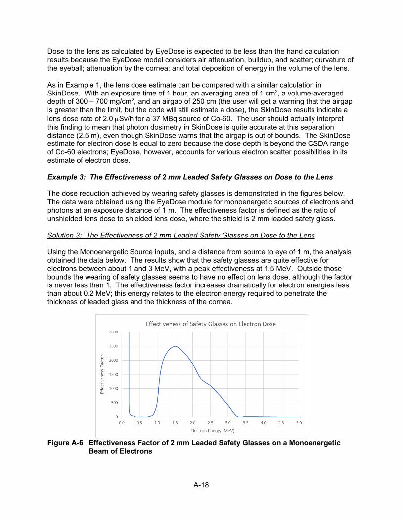
A-18

Dose to the lens as calculated by EyeDose is expected to be less than the hand calculation results because the EyeDose model considers air attenuation, buildup, and scatter; curvature of the eyeball; attenuation by the cornea; and total deposition of energy in the volume of the lens. As in Example 1, the lens dose estimate can be compared with a similar calculation in SkinDose. With an exposure time of 1 hour, an averaging area of 1 cm2, a volume-averaged depth of 300 – 700 mg/cm2, and an airgap of 250 cm (the user will get a warning that the airgap is greater than the limit, but the code will still estimate a dose), the SkinDose results indicate a lens dose rate of 2.0 µSv/h for a 37 MBq source of Co-60. The user should actually interpret this finding to mean that photon dosimetry in SkinDose is quite accurate at this separation distance (2.5 m), even though SkinDose warns that the airgap is out of bounds. The SkinDose estimate for electron dose is equal to zero because the dose depth is beyond the CSDA range of Co-60 electrons; EyeDose, however, accounts for various electron scatter possibilities in its estimate of electron dose. Example 3: The Effectiveness of 2 mm Leaded Safety Glasses on Dose to the Lens The dose reduction achieved by wearing safety glasses is demonstrated in the figures below. The data were obtained using the EyeDose module for monoenergetic sources of electrons and photons at an exposure distance of 1 m. The effectiveness factor is defined as the ratio of unshielded lens dose to shielded lens dose, where the shield is 2 mm leaded safety glass. Solution 3: The Effectiveness of 2 mm Leaded Safety Glasses on Dose to the Lens Using the Monoenergetic Source inputs, and a distance from source to eye of 1 m, the analysis obtained the data below. The results show that the safety glasses are quite effective for electrons between about 1 and 3 MeV, with a peak effectiveness at 1.5 MeV. Outside those bounds the wearing of safety glasses seems to have no effect on lens dose, although the factor is never less than 1. The effectiveness factor increases dramatically for electron energies less than about 0.2 MeV; this energy relates to the electron energy required to penetrate the thickness of leaded glass and the thickness of the cornea.

Figure A-6 Effectiveness Factor of 2 mm Leaded Safety Glasses on a Monoenergetic

Beam of Electrons

A-19

The effectiveness factor as a function of energy for photons shielded by 2 mm leaded safety glass is entirely different than that for electrons. The figure below indicates that the effectiveness in dose reduction for photons less than about 1 MeV is much reduced over that for electrons. It also shows that for energies greater than about 1.3 MeV, wearing safety glasses can actually increase the photon dose to the lens and the glasses are therefore potentially more harmful than helpful. Lens dose is increased by at least a factor of two for photons greater than 4.5 MeV.

Figure A-7 Effectiveness Factor of 2 mm Leaded Safety Glasses on a Monoenergetic

Beam of Photons

31310018C0026

NUREG/CR-6918, Rev 4

Hamby, Mangini, Luitjens, Boozer, Tucker, Rose, Flora

Renaissance Code Development, LLC 310 NW 5th St., Suite 107 Corvallis, Oregon 97330

Office of Nuclear Regulatory Research U.S. Nuclear Regulatory Commission Washington, D.C. 20555-0001

VARSKIN+ is a U.S. Nuclear Regulatory Commission (NRC) computer code to calculate occupational dose to the skin resulting from exposure to radiation emitted from hot particles or other contamination on or near the skin. VARSKIN+ can be used to perform wound dose assessments if the metabolic modeling and dosimetry methods are consistent with NRC regulations. VARSKIN+ gives the user the option to have the code automatically include all decay products in dosimetry calculations or to allow the user to manually add progeny. Both ICRP 38, “Radionuclide Transformations – Energy and Intensity of Emissions” (1983), and ICRP 107, “Nuclear Decay Data for Dosimetry Calculations” (2008), nuclide libraries are available at the user’s option and contain data on gamma rays, X rays, beta particles, internal conversion electrons, and Auger electrons. The photon model accounts for photon attenuation, charged particle buildup, and electron scatter at all depths in skin. The model allows for volumetric sources and clothing or airgaps between source and skin. The electron dosimetry model has a robust accounting for electron energy loss and particle scatter. With the release of VARSKIN+ three new physics modules are introduced: (1) wound dosimetry; (2) neutron dosimetry; and (3) eye dosimetry. Skin and wound dosimetry implement a new alpha dosimetry model for shallow skin assessments.

dosimetry; dose; skin; alpha; beta; gamma; neutron; eye; contamination; shallow

July 2021

Technical

VARSKIN+ 1.0

A Computer Code for Skin Contamination and Dosimetry Assessments

NU

REG

/CR

-6918, Rev 4

VAR

SKIN

+ 1.0 July2021