variational methods in ct reconstruction - part ipcha/hdtomo/sc/week3day1_noise.pdf · variational...
TRANSCRIPT
Variational Methods in CT ReconstructionPart I
Yiqiu Dong
DTU ComputeTechnical University of Denmark
16 Jan. 2017
Yiqiu Dong (DTU Compute) Variational Methods in CT Reconstruction 16 Jan. 2017 1 / 30

1 BackgroundCT ReconstructionInverse ProblemsVariational Methods
2 Reconstruction Based on Gaussian NoiseGaussian NoiseVariational Methods
3 Reconstruction Based on Poisson NoisePoisson NoiseVariational Methods
Yiqiu Dong (DTU Compute) Variational Methods in CT Reconstruction 16 Jan. 2017 2 / 30
Outline
1 BackgroundCT ReconstructionInverse ProblemsVariational Methods
2 Reconstruction Based on Gaussian NoiseGaussian NoiseVariational Methods
3 Reconstruction Based on Poisson NoisePoisson NoiseVariational Methods
Yiqiu Dong (DTU Compute) Variational Methods in CT Reconstruction 16 Jan. 2017 3 / 30

CT Reconstruction
Object
u
May 2014 6/33 P. C. Hanaen: Regularization in Tomography
The Radon Transform
The principle in parallel- beam tomography: send parallel rays through the object at different angles, measure the damping.
f(x) = 2D object / image, x =
·x1x2
¸
f(Á; s) = sinogram / Radon transform
Line integral along line de¯ned by Á and s:
f(Á; s) =
Z 1
¡1f
µs
·cosÁsinÁ
¸+ ¿
·¡ sinÁcosÁ
¸¶d¿
=⇒ measurements
b = N (Au)
Yiqiu Dong (DTU Compute) Variational Methods in CT Reconstruction 16 Jan. 2017 4 / 30

CT Reconstruction
Object
u
May 2014 6/33 P. C. Hanaen: Regularization in Tomography
The Radon Transform
The principle in parallel- beam tomography: send parallel rays through the object at different angles, measure the damping.
f(x) = 2D object / image, x =
·x1x2
¸
f(Á; s) = sinogram / Radon transform
Line integral along line de¯ned by Á and s:
f(Á; s) =
Z 1
¡1f
µs
·cosÁsinÁ
¸+ ¿
·¡ sinÁcosÁ
¸¶d¿
⇐=measurements
b = N (Au)
Our Problem: Reconstruct u from b with given A
It is a highly ill-posed inverse problem
Yiqiu Dong (DTU Compute) Variational Methods in CT Reconstruction 16 Jan. 2017 4 / 30

Inverse Problems
i
10
Reversing a forward problem
Yiqiu Dong (DTU Compute) Variational Methods in CT Reconstruction 16 Jan. 2017 5 / 30

What are inverse problems?
Inverse problem is the question of finding the best representation of therequired states from the given measurements, together with anyappropriate prior information that may be available about the states andthe measuring device.
Yiqiu Dong (DTU Compute) Variational Methods in CT Reconstruction 16 Jan. 2017 6 / 30

Questions need be thought about
Why are inverse problems difficult?I Forward models are not explicitly invertibleI Errors in the measurement (and also in the forward model) can lead to
errors in the solution
Yiqiu Dong (DTU Compute) Variational Methods in CT Reconstruction 16 Jan. 2017 7 / 30

Questions need be thought about
Why are inverse problems difficult?I Forward models are not explicitly invertible
F Existence: Does any state fit the measurement?F Uniqueness: Is there a unique state vector fits the measurement?
I Errors in the measurement (and also in the forward model) can lead toerrors in the solution
F Stability: Can small changes in the measurement produce large changesin the solution?
Yiqiu Dong (DTU Compute) Variational Methods in CT Reconstruction 16 Jan. 2017 7 / 30

Hadamard Condition
A problem is called well-posed if
1 there exists a solution to the problem (existence),
2 there is at most one solution to the problem (uniqueness),
3 the solution depends continuously on the measurement (stability).
Otherwise the problem is called ill-posed.
Yiqiu Dong (DTU Compute) Variational Methods in CT Reconstruction 16 Jan. 2017 8 / 30

Example
Object
u
May 2014 6/33 P. C. Hanaen: Regularization in Tomography
The Radon Transform
The principle in parallel- beam tomography: send parallel rays through the object at different angles, measure the damping.
f(x) = 2D object / image, x =
·x1x2
¸
f(Á; s) = sinogram / Radon transform
Line integral along line de¯ned by Á and s:
f(Á; s) =
Z 1
¡1f
µs
·cosÁsinÁ
¸+ ¿
·¡ sinÁcosÁ
¸¶d¿
=⇒ measurements
b = N (Au)
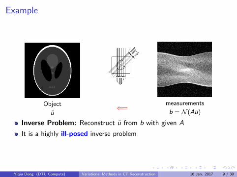
Forward Problem: Send X-rays through the object at differentangles, and measure the damping
Yiqiu Dong (DTU Compute) Variational Methods in CT Reconstruction 16 Jan. 2017 9 / 30
Example
Object
u
May 2014 6/33 P. C. Hanaen: Regularization in Tomography
The Radon Transform
The principle in parallel- beam tomography: send parallel rays through the object at different angles, measure the damping.
f(x) = 2D object / image, x =
·x1x2
¸
f(Á; s) = sinogram / Radon transform
Line integral along line de¯ned by Á and s:
f(Á; s) =
Z 1
¡1f
µs
·cosÁsinÁ
¸+ ¿
·¡ sinÁcosÁ
¸¶d¿
⇐=measurements
b = N (Au)
Inverse Problem: Reconstruct u from b with given A
It is a highly ill-posed inverse problem
Yiqiu Dong (DTU Compute) Variational Methods in CT Reconstruction 16 Jan. 2017 9 / 30
More Questions Need Be Thought About
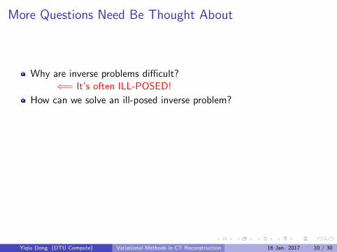
Why are inverse problems difficult?⇐= It’s often ILL-POSED!
How can we solve an ill-posed inverse problem?
I Does the measurements actually contain the information we want?I Which of an infinite manifold of solutions do we want?I The measurement may not be enough by itself to completely determine
the unknown. What other prior information of the “unknown” do wehave?
⇐= We can use REGULARIZATION techniques! (Tomorrow)
Yiqiu Dong (DTU Compute) Variational Methods in CT Reconstruction 16 Jan. 2017 10 / 30

More Questions Need Be Thought About
Why are inverse problems difficult?⇐= It’s often ILL-POSED!
How can we solve an ill-posed inverse problem?I Does the measurements actually contain the information we want?I Which of an infinite manifold of solutions do we want?I The measurement may not be enough by itself to completely determine
the unknown. What other prior information of the “unknown” do wehave?
⇐= We can use REGULARIZATION techniques! (Tomorrow)
Yiqiu Dong (DTU Compute) Variational Methods in CT Reconstruction 16 Jan. 2017 10 / 30

Variational Method
The variational method to imaging science constitutes thecomputation of a reconstructed image u based on the measurements bas a minimizer of a functional, which is called as a variational model.
Variational methods play an important role in inverse problems.
The modelling of the variational method can be best motivated fromBayesian statistics.
Yiqiu Dong (DTU Compute) Variational Methods in CT Reconstruction 16 Jan. 2017 11 / 30

Variational Method
Two key challenges:1 Good variational model: minu E (u).
I The goal is to construct an E (·) that describes the “quality” of thereconstruction.
F Bad reconstruction = Large value of E(·)F Good reconstruction = small value of E(·)
I Existence, uniqueness, etc..
2 Efficient optimization algorithm.
I The goal is to find an easily implemented algorithm to solve thevariational model with low computation and high accuracy.
I Convexity, relaxation, convergence, parallazation, etc..
Yiqiu Dong (DTU Compute) Variational Methods in CT Reconstruction 16 Jan. 2017 12 / 30

Variational Method
Two key challenges:1 Good variational model: minu E (u).
I The goal is to construct an E (·) that describes the “quality” of thereconstruction.
F Bad reconstruction = Large value of E(·)F Good reconstruction = small value of E(·)
I Existence, uniqueness, etc..
2 Efficient optimization algorithm.I The goal is to find an easily implemented algorithm to solve the
variational model with low computation and high accuracy.I Convexity, relaxation, convergence, parallazation, etc..
Yiqiu Dong (DTU Compute) Variational Methods in CT Reconstruction 16 Jan. 2017 12 / 30

Variational Model
minu∈U
F(u, b) + γR(u)
F(·, b) is the data-fitting (or data-fidelity) term, which keep theestimation of u close to the data b under the forward physical system.It is usually based on the noise model.
R(·) is the regularization term, which commonly depends on the priorinformation of u.
γ > 0 is the regularization parameter, which controls the trade-offbetween a good fit of b and the requirement from the regularization.
Yiqiu Dong (DTU Compute) Variational Methods in CT Reconstruction 16 Jan. 2017 13 / 30

Outline
1 BackgroundCT ReconstructionInverse ProblemsVariational Methods
2 Reconstruction Based on Gaussian NoiseGaussian NoiseVariational Methods
3 Reconstruction Based on Poisson NoisePoisson NoiseVariational Methods
Yiqiu Dong (DTU Compute) Variational Methods in CT Reconstruction 16 Jan. 2017 14 / 30
Gaussian Noise
b = Au + η.
u ∈ Rn×n is the true image.
b ∈ Rr×p is the measurements, where r denotes the number ofdetector pixels and p is the number of projections.
A : Rn×n → Rr×p denotes the Radon transform as an operator.
η ∈ Rrp is additive white Gaussian noise. Each ηi can be seen as aGaussian random variable with mean 0 and variance σ2, and all ηi areindependent. η is also independent on u. The probability distributionfunction (PDF) is given by
p(ηi = a) =1√2πσ
e−a2
2σ2 .
Yiqiu Dong (DTU Compute) Variational Methods in CT Reconstruction 16 Jan. 2017 15 / 30
Gaussian Noise
b = Au + η.
u ∈ Rn2 is the object.
b ∈ Rrp is the measurements, where r denotes the number of detectorpixels and p is the number of projections.
A ∈ Rrp×n2 denotes the Radon transform in matrix format.
η ∈ Rrp is additive white Gaussian noise. Each ηi can be seen as aGaussian random variable with mean 0 and variance σ2, and all ηi areindependent. η is also independent on u. The probability distributionfunction (PDF) is given by
p(ηi = a) =1√2πσ
e−a2
2σ2 .
Yiqiu Dong (DTU Compute) Variational Methods in CT Reconstruction 16 Jan. 2017 15 / 30

Naive Solution
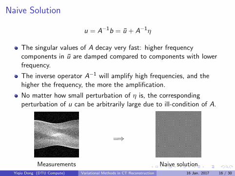
u = A−1b = u + A−1η
The singular values of A decay very fast: higher frequencycomponents in u are damped compared to components with lowerfrequency.
The inverse operator A−1 will amplify high frequencies, and thehigher the frequency, the more the amplification.
No matter how small perturbation of η is, the correspondingperturbation of u can be arbitrarily large due to ill-condition of A.
Measurements
=⇒
The results of our algorithm
The “naıve” reconstruction of the pumpkin image, obtained by computingX = Ac
�1BAr�T via Gaussian elimination on both Ac and Ar. The image
X is completely dominated by the influence of the noise.
21
Naive solution
Yiqiu Dong (DTU Compute) Variational Methods in CT Reconstruction 16 Jan. 2017 16 / 30
Naive Solution
u = A−1b = u + A−1η
The singular values of A decay very fast: higher frequencycomponents in u are damped compared to components with lowerfrequency.
The inverse operator A−1 will amplify high frequencies, and thehigher the frequency, the more the amplification.
No matter how small perturbation of η is, the correspondingperturbation of u can be arbitrarily large due to ill-condition of A.
Measurements
=⇒
The results of our algorithm
The “naıve” reconstruction of the pumpkin image, obtained by computingX = Ac
�1BAr�T via Gaussian elimination on both Ac and Ar. The image
X is completely dominated by the influence of the noise.
21
Naive solutionYiqiu Dong (DTU Compute) Variational Methods in CT Reconstruction 16 Jan. 2017 16 / 30

Variational Model
Consider a set of random variables U. Each element Ui of U is corruptedby an independent Gaussian random variable Ni with Gaussian distributionN0,σ2 . The observed image is a set of random variables B with intensityBi = (AU)i + Ni at each i ∈ {1, · · · , rp}. The problem is to reconstruct Ufrom B, that is, we wish to determine the object u which is the most likelygiven the measurement b, i.e.,
maxu
P(U = u|B = b).
Yiqiu Dong (DTU Compute) Variational Methods in CT Reconstruction 16 Jan. 2017 17 / 30
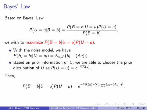
Bayes’ Law
Based on Bayes’ Law
P(U = u|B = b) =P(B = b|U = u)P(U = u)
P(B = b),
we wish to maximize P(B = b|U = u)P(U = u).
With the noise model, we haveP(Bi = bi |Ui = ui ) = N0,σ2(bi − (Au)i ).
Based on prior information of U, we are able to choose the priordistribution of U as P(U = u) = e−γR(u).
Then,
P(B = b|U = u)P(U = u) = e−γR(u)−∑
i1
2σ2 (bi−(Au)i )2 .
Yiqiu Dong (DTU Compute) Variational Methods in CT Reconstruction 16 Jan. 2017 18 / 30

Variational Model
maxu
P(U = u|B = b)⇐⇒ maxu
P(B = b|U = u)P(U = u)
⇐⇒ minu− ln(P(B = b|U = u)P(U = u))
⇐⇒ minu
1
2
∑
i
(bi − (Au)i )2 + γσ2R(u)
⇐⇒ minu
1
2‖b − Au‖22 + γR(u)
Yiqiu Dong (DTU Compute) Variational Methods in CT Reconstruction 16 Jan. 2017 19 / 30

Variational Model
Today, we only consider the Tikhonov regularization, i.e., R(u) = 12‖u‖22.
Then the variational model for X-ray reconstruction under the Gaussiannoise is
minu
1
2‖b − Au‖22 +
γ
2‖u‖22
The minimizer u should satisfy the first-order condition:
0 = A>(Au − b) + γu
Yiqiu Dong (DTU Compute) Variational Methods in CT Reconstruction 16 Jan. 2017 20 / 30

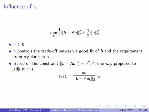
Influence of γ
minu
1
2‖b − Au‖22 +
γ
2‖u‖22
γ > 0
γ controls the trade-off between a good fit of b and the requirementfrom regularization
Based on the constraint ‖b − Au‖22 = σ2n2, one way proposed toadjust γ is
γk+1 =nσ
‖b − Auk‖2γk
Yiqiu Dong (DTU Compute) Variational Methods in CT Reconstruction 16 Jan. 2017 21 / 30

Example
Object Measurements
0
0.2
0.4
0.6
Result with γ = 1000
-0.5
0
0.5
1
Result with γ = 100
Yiqiu Dong (DTU Compute) Variational Methods in CT Reconstruction 16 Jan. 2017 22 / 30

Outline
1 BackgroundCT ReconstructionInverse ProblemsVariational Methods
2 Reconstruction Based on Gaussian NoiseGaussian NoiseVariational Methods
3 Reconstruction Based on Poisson NoisePoisson NoiseVariational Methods
Yiqiu Dong (DTU Compute) Variational Methods in CT Reconstruction 16 Jan. 2017 23 / 30

Poisson Noise
Poisson noise commonly exists in measurements through a photonscounting operation, such as from digital camera, confocal microscopy,PET and SPECT tomography.
Poisson noise is signal dependent.
In X-ray tomography, the value of the measurement bi denotes thecounting number of photons, so it follows Poisson noise model.Usually we assume b is bounded, positive, integer valued (but this willultimately be unnecessary), and bi at different points are independent.
Yiqiu Dong (DTU Compute) Variational Methods in CT Reconstruction 16 Jan. 2017 24 / 30
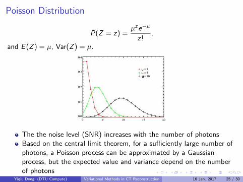
Poisson Distribution
P(Z = z) =µze−µ
z!,
and E (Z ) = µ, Var(Z ) = µ.
The the noise level (SNR) increases with the number of photonsBased on the central limit theorem, for a sufficiently large number ofphotons, a Poisson process can be approximated by a Gaussianprocess, but the expected value and variance depend on the numberof photons
Yiqiu Dong (DTU Compute) Variational Methods in CT Reconstruction 16 Jan. 2017 25 / 30

Example
84 CHAPTER 5. DENOISING WITH THRESHOLDING
�max = 5 �max = 50 �max = 50 �max = 100
Figure 5.28: Noisy image with Poisson noise model, for various �max = maxn f0[n].
to f might give poor results since the noise level fluctuates from point to point, and thus a singlethreshold T might not be able to capture these variations. A simple way to improve the thresholdingresults is to first apply a variance stabilization non-linearity � : R ! R to the image, so that �(f)is as close as possible to an additive Gaussian white noise model
�(f) ⇡ �(f0) + w (5.8)
where w[n] ⇠ N (0,�) is a Gaussian white noise of fixed variance �2.Perfect stabilization is impossible, so that (5.8) only approximately holds for a limited intensity
range of f0[n]. Two popular variation stabilization functions for Poisson noise are the Anscombemapping
�(x) = 2p
x + 3/8
and the mapping of Freeman and Tukey
�(x) =p
x + 1 +p
x.
Figure 5.29 shows the e�ect of these variance stabilizations on the variance of �(f).
1 2 3 4 5 6 7 8 9 10
0.75
0.8
0.85
0.9
0.95
1
1.05
Figure 5.29: Comparison of variariance stabilization: display of Var(�(f [n])) as a function of f0[n].
A variance stabilized denoiser is defined as
�stab,q(f) = ��1(X
m
SqT (h�(f), mi) m)
where ��1 is the inverse mapping of �.Figure 5.30 shows that for moderate intensity range, variance stabilization improves over non-
stabilized denoising.
5.5 Multiplicative NoiseMultiplicative image formation. A multiplicative noise model assumes that
f [n] = f0[n]w[n]
umax = 5 umax = 25 umax = 50 umax = 100
Yiqiu Dong (DTU Compute) Variational Methods in CT Reconstruction 16 Jan. 2017 26 / 30

Poisson Noise in X-ray
According to the Lambert-Beer law, the number of transmitted photons(per second per unit area) is
B = B0e−
∫l µ(x) ds
where B0 denotes the incident photon flux, which is known.
But both the X-ray generation process and the absorption/attenuationprocess are stochastic processes. The reality of B would follow Poissondistribution, i.e.,
Yiqiu Dong (DTU Compute) Variational Methods in CT Reconstruction 16 Jan. 2017 27 / 30

Poisson Noise in X-ray
According to the Lambert-Beer law, the number of transmitted photons(per second per unit area) is
Bi = B0e−(Au)i ∀i
where B0 denotes the incident photon flux, which is known.
But both the X-ray generation process and the absorption/attenuationprocess are stochastic processes. The reality of B would follow Poissondistribution, i.e.,
Bi ∼ Poisson(B0e−(Au)i ) ∀i
Yiqiu Dong (DTU Compute) Variational Methods in CT Reconstruction 16 Jan. 2017 27 / 30

Poisson Noise in X-ray
According to the Lambert-Beer law, the number of transmitted photons(per second per unit area) is
Bi = B0e−(Au)i ∀i
where B0 denotes the incident photon flux, which is known.
But both the X-ray generation process and the absorption/attenuationprocess are stochastic processes. The reality of B would follow Poissondistribution, i.e.,
P(Bi = bi |U = u) =(B0e
−(Au)i )bi
bi !e−(B0e
−(Au)i ) ∀i
Yiqiu Dong (DTU Compute) Variational Methods in CT Reconstruction 16 Jan. 2017 27 / 30
Variational Model
For Poisson noise removal, we wish to determine the object u that is mostlikely given the measurements b, i.e., maxu P(U = u|B = b).
Based on Bayes’ Law
P(U = u|B = b) =P(B = b|U = u)P(U = u)
P(B = b),
we wish to maximize P(B = b|U = u)P(U = u).
With the Poisson noise model, for each i we have
P(Bi = bi |U = u) =(B0e
−(Au)i )bi
bi !e−(B0e
−(Au)i )
Based on prior information of U, we are able to choose the priordistribution of U as P(U = u) = e−γR(u), e.g. P(U = u) = e−γ‖u‖
22
Yiqiu Dong (DTU Compute) Variational Methods in CT Reconstruction 16 Jan. 2017 28 / 30

Variational Model
For Poisson noise removal, we wish to determine the object u that is mostlikely given the measurements b, i.e., maxu P(U = u|B = b).Based on Bayes’ Law
P(U = u|B = b) =P(B = b|U = u)P(U = u)
P(B = b),
we wish to maximize P(B = b|U = u)P(U = u).
With the Poisson noise model, for each i we have
P(Bi = bi |U = u) =(B0e
−(Au)i )bi
bi !e−(B0e
−(Au)i )
Based on prior information of U, we are able to choose the priordistribution of U as P(U = u) = e−γR(u), e.g. P(U = u) = e−γ‖u‖
22
Yiqiu Dong (DTU Compute) Variational Methods in CT Reconstruction 16 Jan. 2017 28 / 30

Variational Model
Instead of maximizing P(B = b|U = u)P(U = u), we minimize− log(P(B = b|U = u)P(U = u)), and we obtain the variational model forX-ray reconstruction under Poisson noise
minu
∑
i
(bi (Au)i + B0e
−(Au)i)
+ γR(u)
The minimizer u should satisfy the first-order condition:
0 = A>(b − B0e
−Au)
+ γu
Yiqiu Dong (DTU Compute) Variational Methods in CT Reconstruction 16 Jan. 2017 29 / 30

Variational Model
Instead of maximizing P(B = b|U = u)P(U = u), we minimize− log(P(B = b|U = u)P(U = u)), and we obtain the variational model forX-ray reconstruction under Poisson noise
minu
∑
i
(bi (Au)i + B0e
−(Au)i)
+γ
2‖u‖22
The minimizer u should satisfy the first-order condition:
0 = A>(b − B0e
−Au)
+ γu
Yiqiu Dong (DTU Compute) Variational Methods in CT Reconstruction 16 Jan. 2017 29 / 30

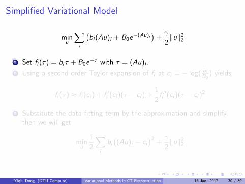
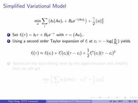
Simplified Variational Model
minu
∑
i
(bi (Au)i + B0e
−(Au)i)
+γ
2‖u‖22
1 Set fi (τ) = biτ + B0e−τ with τ = (Au)i .
2 Using a second order Taylor expansion of fi at ci = − log( biB0
) yields
fi (τ) ≈ fi (ci ) + f ′i (ci )(τ − ci ) +1
2f ′′i (ci )(τ − ci )
2
3 Substitute the data-fitting term by the approximation and simplify,then we will get
minu
1
2
∑
i
bi((Au)i − ci
)2+γ
2‖u‖22
Yiqiu Dong (DTU Compute) Variational Methods in CT Reconstruction 16 Jan. 2017 30 / 30