variational learning for switching state-space …mlg.eng.cam.ac.uk/pub/pdf/ghahin00a.pdfswitching...

LETTER Communicated by Volker Tresp

Variational Learning for Switching State-Space Models

Zoubin GhahramaniGeoffrey E. HintonGatsby Computational Neuroscience Unit, University College London, London WC1N3AR, U.K.

We introduce a new statistical model for time series that iteratively seg-ments data into regimes with approximately linear dynamics and learnsthe parameters of each of these linear regimes. This model combines andgeneralizes two of the most widely used stochastic time-series models—hidden Markov models and linear dynamical systems—and is closelyrelated to models that are widely used in the control and econometricsliteratures. It can also be derived by extending the mixture of expertsneural network (Jacobs, Jordan, Nowlan, & Hinton, 1991) to its fully dy-namical version, in which both expert and gating networks are recurrent.Inferring the posterior probabilities of the hidden states of this modelis computationally intractable, and therefore the exact expectation maxi-mization (EM) algorithm cannot be applied. However, we present a varia-tional approximation that maximizes a lower bound on the log-likelihoodand makes use of both the forward and backward recursions for hiddenMarkov models and the Kalman filter recursions for linear dynamical sys-tems. We tested the algorithm on artificial data sets and a natural data setof respiration force from a patient with sleep apnea. The results suggestthat variational approximations are a viable method for inference andlearning in switching state-space models.

1 Introduction

Most commonly used probabilistic models of time series are descendantsof either hidden Markov models (HMM) or stochastic linear dynamicalsystems, also known as state-space models (SSM). HMMs represent in-formation about the past of a sequence through a single discrete randomvariable—the hidden state. The prior probability distribution of this state isderived from the previous hidden state using a stochastic transition matrix.Knowing the state at any time makes the past, present, and future observa-tions statistically independent. This is the Markov independence propertythat gives the model its name.

SSMs represent information about the past through a real-valued hiddenstate vector. Again, conditioned on this state vector, the past, present, andfuture observations are statistically independent. The dependency between

Neural Computation 12, 831–864 (2000) c© 2000 Massachusetts Institute of Technology

832 Zoubin Ghahramani and Geoffrey E. Hinton

the present state vector and the previous state vector is specified throughthe dynamic equations of the system and the noise model. When theseequations are linear and the noise model is gaussian, the SSM is also knownas a linear dynamical system or Kalman filter model.

Unfortunately, most real-world processes cannot be characterized by ei-ther purely discrete or purely linear-gaussian dynamics. For example, anindustrial plant may have multiple discrete modes of behavior, each withapproximately linear dynamics. Similarly, the pixel intensities in an imageof a translating object vary according to approximately linear dynamicsfor subpixel translations, but as the image moves over a larger range, thedynamics change significantly and nonlinearly.

This article addresses models of dynamical phenomena that are charac-terized by a combination of discrete and continuous dynamics. We intro-duce a probabilistic model called the switching SSM inspired by the divide-and-conquer principle underlying the mixture-of-experts neural network(Jacobs, Jordan, Nowlan, & Hinton, 1991). Switching SSMs are a naturalgeneralization of HMMs and SSMs in which the dynamics can transition ina discrete manner from one linear operating regime to another. There is alarge literature on models of this kind in econometrics, signal processing,and other fields (Harrison & Stevens, 1976; Chang & Athans, 1978; Hamil-ton, 1989; Shumway & Stoffer, 1991; Bar-Shalom & Li, 1993). Here we extendthese models to allow for multiple real-valued state vectors, draw connec-tions between these fields and the relevant literature on neural computationand probabilistic graphical models, and derive a learning algorithm for allthe parameters of the model based on a structured variational approxima-tion that rigorously maximizes a lower bound on the log-likelihood.

In the following section we review the background material on SSMs,HMMs, and hybrids of the two. In section 3, we describe the generativemodel—the probability distribution defined over the observation se-quences—for switching SSMs. In section 4, we describe a learning algorithmfor switching state-space models that is based on a structured variationalapproximation to the expectation-maximization algorithm. In section 5 wepresent simulation results in both an artificial domain, to assess the qualityof the approximate inference method, and a natural domain. We concludewith section 6.

2 Background

2.1 State-Space Models. An SSM defines a probability density over timeseries of real-valued observation vectors {Yt} by assuming that the obser-vations were generated from a sequence of hidden state vectors {Xt}. (Ap-pendix A describes the variables and notation used throughout this article.)In particular, the SSM specifies that given the hidden state vector at onetime step, the observation vector at that time step is statistically indepen-dent from all other observation vectors, and that the hidden state vectors

Switching State-Space Models 833

XX1

Y Y1

X

Y

2

2

X3

Y3

...T

T

Figure 1: A directed acyclic graph (DAG) specifying conditional independencerelations for a state-space model. Each node is conditionally independent fromits nondescendants given its parents. The output Yt is conditionally independentfrom all other variables given the state Xt; and Xt is conditionally independentfrom X1, . . . ,Xt−2 given Xt−1. In this and the following figures, shaded nodesrepresent observed variables, and unshaded nodes represent hidden variables.

obey the Markov independence property. The joint probability for the se-quences of states Xt and observations Yt can therefore be factored as:

P({Xt,Yt}) = P(X1)P(Y1|X1)

T∏t=2

P(Xt|Xt−1)P(Yt|Xt). (2.1)

The conditional independencies specified by equation 2.1 can be expressedgraphically in the form of Figure 1. The simplest and most commonly usedmodels of this kind assume that the transition and output functions arelinear and time invariant and the distributions of the state and observationvariables are multivariate gaussian. We use the term state-space model torefer to this simple form of the model. For such models, the state transitionfunction is

Xt = AXt−1 + wt, (2.2)

where A is the state transition matrix and wt is zero-mean gaussian noise inthe dynamics, with covariance matrix Q. P(X1) is assumed to be gaussian.Equation 2.2 ensures that if P(Xt−1) is gaussian, so is P(Xt). The outputfunction is

Yt = CXt + vt, (2.3)

where C is the output matrix and vt is zero-mean gaussian output noisewith covariance matrix R; P(Yt|Xt) is therefore also gaussian:

P(Yt|Xt) = (2π)−D/2|R|−1/2 exp{−1

2(Yt − CXt)

′ R−1 (Yt − CXt)

}, (2.4)

where D is the dimensionality of the Y vectors.


Often the observation vector can be divided into input (or predictor)variables and output (or response) variables. To model the input-outputbehavior of such a system—the conditional probability of output sequencesgiven input sequences—the linear gaussian SSM can be modified to have astate-transition function,

Xt = AXt−1 + BUt + wt, (2.5)

where Ut is the input observation vector and B is the (fixed) input matrix.1

The problem of inference or state estimation for an SSM with known pa-rameters consists of estimating the posterior probabilities of the hiddenvariables given a sequence of observed variables. Since the local likelihoodfunctions for the observations are gaussian and the priors for the hiddenstates are gaussian, the resulting posterior is also gaussian. Three specialcases of the inference problem are often considered: filtering, smoothing,and prediction (Anderson & Moore, 1979; Goodwin & Sin, 1984). The goalof filtering is to compute the probability of the current hidden state Xt giventhe sequence of inputs and outputs up to time t—P(Xt|{Y}t1, {U}t1).2 The re-cursive algorithm used to perform this computation is known as the Kalmanfilter (Kalman & Bucy, 1961). The goal of smoothing is to compute the prob-ability of Xt given the sequence of inputs and outputs up to time T, whereT > t. The Kalman filter is used in the forward direction to compute theprobability of Xt given {Y}t1 and {U}t1. A similar set of backward recursionsfrom T to t completes the computation by accounting for the observationsafter time t (Rauch, 1963). We will refer to the combined forward and back-ward recursions for smoothing as the Kalman smoothing recursions (alsoknown as the RTS, or Rauch-Tung-Streibel smoother). Finally, the goal ofprediction is to compute the probability of future states and observationsgiven observations up to time t. Given P(Xt|{Y}t1, {U}t1) computed as before,the model is simulated in the forward direction using equations 2.2 (or 2.5if there are inputs) and 2.3 to compute the probability density of the stateor output at future time t+ τ .

The problem of learning the parameters of an SSM is known in engineer-ing as the system identification problem; in its most general form it assumesaccess only to sequences of input and output observations. We focus on max-imum likelihood learning in which a single (locally optimal) value of the pa-rameters is estimated, rather than Bayesian approaches that treat the param-eters as random variables and compute or approximate the posterior distri-bution of the parameters given the data. One can also distinguish betweenon-line and off-line approaches to learning. On-line recursive algorithms,favored in real-time adaptive control applications, can be obtained by com-puting the gradient or the second derivatives of the log-likelihood (Ljung

1 One can also define the state such that Xt+1 = AXt + BUt + wt.2 The notation {Y}t1 is shorthand for the sequence Y1, . . . ,Yt.


& Soderstrom, 1983). Similar gradient-based methods can be obtained foroff-line methods. An alternative method for off-line learning makes use ofthe expectation maximization (EM) algorithm (Dempster, Laird, & Rubin,1977). This procedure iterates between an E-step that fixes the current pa-rameters and computes posterior probabilities over the hidden states giventhe observations, and an M-step that maximizes the expected log-likelihoodof the parameters using the posterior distribution computed in the E-step.For linear gaussian state-space models, the E-step is exactly the Kalmansmoothing problem as defined above, and the M-step simplifies to a lin-ear regression problem (Shumway & Stoffer, 1982; Digalakis, Rohlicek, &Ostendorf, 1993). Details on the EM algorithm for SSMs can be found inGhahramani and Hinton (1996a), as well as in the original Shumway andStoffer (1982) article.

2.2 Hidden Markov Models. Hidden Markov models also define prob-ability distributions over sequences of observations {Yt}. The distributionover sequences is obtained by specifying a distribution over observationsat each time step t given a discrete hidden state St, and the probability oftransitioning from one hidden state to another. Using the Markov property,the joint probability for the sequences of states St and observations Yt, canbe factored in exactly the same manner as equation 2.1, with St taking theplace of Xt:

P({St,Yt}) = P(S1)P(Y1|S1)

T∏t=2

P(St|St−1)P(Yt|St). (2.6)

Similarly, the conditional independencies in an HMM can be expressedgraphically in the same form as Figure 1. The state is represented by a singlemultinomial variable that can take one of K discrete values, St ∈ {1, . . . ,K}.The state transition probabilities, P(St|St−1), are specified by a K × K tran-sition matrix. If the observables are discrete symbols taking on one of Lvalues, the observation probabilities P(Yt|St) can be fully specified as aK× L observation matrix. For a continuous observation vector, P(Yt|St) canbe modeled in many different forms, such as a gaussian, mixture of gaus-sians, or neural network. HMMs have been applied extensively to prob-lems in speech recognition (Juang & Rabiner, 1991), computational biology(Baldi, Chauvin, Hunkapiller, & McClure, 1994), and fault detection (Smyth,1994).

Given an HMM with known parameters and a sequence of observations,two algorithms are commonly used to solve two different forms of the in-ference problem (Rabiner & Juang, 1986). The first computes the posteriorprobabilities of the hidden states using a recursive algorithm known as theforward-backward algorithm. The computations in the forward pass are ex-actly analogous to the Kalman filter for SSMs, and the computations in thebackward pass are analogous to the backward pass of the Kalman smoothing


equations. As noted by Bridle (pers. comm., 1985) and Smyth, Heckerman,and Jordan (1997), the forward-backward algorithm is a special case of exactinference algorithms for more general graphical probabilistic models (Lau-ritzen & Spiegelhalter, 1988; Pearl, 1988). The same observation holds truefor the Kalman smoothing recursions. The other inference problem com-monly posed for HMMs is to compute the single most likely sequence ofhidden states. The solution to this problem is given by the Viterbi algorithm,which also consists of a forward and backward pass through the model.

To learn maximum likelihood parameters for an HMM given sequencesof observations, one can use the well-known Baum-Welch algorithm (Baum,Petrie, Soules, & Weiss, 1970). This algorithm is a special case of EM thatuses the forward-backward algorithm to infer the posterior probabilities ofthe hidden states in the E-step. The M-step uses expected counts of tran-sitions and observations to reestimate the transition and output matrices(or linear regression equations in the case where the observations are gaus-sian distributed). Like SSMs, HMMs can be augmented to allow for inputvariables, such that they model the conditional distribution of sequences ofoutput observations given sequences of inputs (Cacciatore & Nowlan, 1994;Bengio & Frasconi, 1995; Meila & Jordan, 1996).

2.3 Hybrids. A burgeoning literature on models that combine the dis-crete transition structure of HMMs with the linear dynamics of SSMs hasdeveloped in fields ranging from econometrics to control engineering (Har-rison & Stevens, 1976; Chang & Athans, 1978; Hamilton, 1989; Shumway& Stoffer, 1991; Bar-Shalom & Li, 1993; Deng, 1993; Kadirkamanathan &Kadirkamanathan, 1996; Chaer, Bishop, & Ghosh, 1997). These models areknown alternately as hybrid models, SSMs with switching, and jump-linearsystems. We briefly review some of this literature, including some relatedneural network models.3

Shortly after Kalman and Bucy solved the problem of state estimationfor linear gaussian SSMs, attention turned to the analogous problem forswitching models (Ackerson & Fu, 1970). Chang and Athans (1978) derivethe equations for computing the conditional mean and variance of the statewhen the parameters of a linear SSM switch according to arbitrary andMarkovian dynamics. The prior and transition probabilities of the switchingprocess are assumed to be known. They note that for M models (sets ofparameters) and an observation length T, the exact conditional distributionof the state is a gaussian mixture with MT components. The conditionalmean and variance, which require far less computation, are therefore onlysummary statistics.

3 A review of how SSMs and HMMs are related to simpler statistical models such asprincipal components analysis, factor analysis, mixture of gaussians, vector quantization,and independent components analysis (ICA) can be found in Roweis and Ghahramani(1999).


Y Y Y ...1 2 3

a

c

b

d

S S

X X

Y Y Y

...

...

...

1

1 2 3

3X2

2S 31

S

X

Y Y Y

...

...

...1 2 3

32X1X

1 S2 S3

S S

X

...

...X2 3

3S21

X1

...1 2 3U U U

S S

X

Y Y Y

...

...

...1 2 3

X2 3

3S21

X1

Figure 2: Directed acyclic graphs specifying conditional independence relationsfor various switching state-space models. (a) Shumway and Stoffer (1991): theoutput matrix (C in equation 2.3) switches independently between a fixed num-ber of choices at each time step. Its setting is represented by the discrete hiddenvariable St; (b) Bar-Shalom and Li (1993): both the output equation and thedynamic equation can switch, and the switches are Markov; (c) Kim (1994);(d) Fraser and Dimitriadis (1993): outputs and states are observed. Here wehave shown a simple case where the output depends directly on the currentstate, previous state, and previous output.

Shumway and Stoffer (1991) consider the problem of learning the param-eters of SSMs with a single real-valued hidden state vector and switchingoutput matrices. The probability of choosing a particular output matrix isa prespecified time-varying function, independent of previous choices (seeFigure 2a). A pseudo-EM algorithm is derived in which the E-step, which


in its exact form would require computing a gaussian mixture with MT

components, is approximated by a single gaussian at each time step.Bar-Shalom and Li (1993; sec. 11.6) review models in which both the state

dynamics and the output matrices switch, and where the switching followsMarkovian dynamics (see Figure 2b). They present several methods for ap-proximately solving the state-estimation problem in switching models (theydo not discuss parameter estimation for such models). These methods, re-ferred to as generalized pseudo-Bayesian (GPB) and interacting multiplemodels (IMM), are all based on the idea of collapsing into one gaussianthe mixture of M gaussians that results from considering all the settings ofthe switch state at a given time step. This avoids the exponential growthof mixture components at the cost of providing an approximate solution.More sophisticated but computationally expensive methods that collapseM2 gaussians into M gaussians are also derived. Kim (1994) derives a simi-lar approximation for a closely related model, which also includes observedinput variables (see Figure 2c). Furthermore, Kim discusses parameter es-timation for this model, although without making reference to the EM al-gorithm. Other authors have used Markov chain Monte Carlo methods forstate and parameter estimation in switching models (Carter & Kohn, 1994;Athaide, 1995) and in other related dynamic probabilistic networks (Dean& Kanazawa, 1989; Kanazawa, Koller, & Russell, 1995).

Hamilton (1989, 1994, sec. 22.4) describes a class of switching modelsin which the real-valued observation at time t, Yt, depends on both theobservations at times t−1 to t−r and the discrete states at time t to t−r. Moreprecisely, Yt is gaussian with mean that is a linear function of Yt−1, . . . ,Yt−rand of binary indicator variables for the discrete states, St, . . . ,St−r. Thesystem can therefore be seen as an (r + 1)th order HMM driving an rthorder autoregressive process, and is tractable for small r and number ofdiscrete states in S.

Hamilton’s models are closely related to hidden filter HMM (HFHMM;Fraser & Dimitriadis, 1993). HFHMMs have both discrete and real-valuedstates. However, the real-valued states are assumed to be either observed or aknown, deterministic function of the past observations (i.e., an embedding).The outputs depend on the states and previous outputs, and the form ofthis dependence can switch randomly (see Figure 2d). Because at any timestep the only hidden variable is the switch state, St, exact inference in thismodel can be carried out tractably. The resulting algorithm is a variant ofthe forward-backward procedure for HMMs. Kehagias and Petridis (1997)and Pawelzik, Kohlmorgen, and Muller (1996) present other variants of thismodel.

Elliott, Aggoun, and Moore (1995; sec. 12.5) present an inference algo-rithm for hybrid (Markov switching) systems for which there is a separateobservable from which the switch state can be estimated. The true switchstates, St, are represented as unit vectors in <M, and the estimated switchstate is a vector in the unit square with elements corresponding to the es-


timated probability of being in each switch state. The real-valued state, Xt,is approximated as a gaussian given the estimated switch state by forminga linear combination of the transition and observation matrices for the dif-ferent SSMs weighted by the estimated switch state. Eliott et al. also derivecontrol equations for such hybrid systems and discuss applications of thechange-of-measures whitening procedure to a large family of models.

With regard to the literature on neural computation, the model presentedin this article is a generalization of both the mixture-of-experts neural net-work (Jacobs et al., 1991; Jordan & Jacobs, 1994) and the related mixtureof factor analyzers (Hinton, Dayan, & Revow, 1997; Ghahramani & Hin-ton, 1996b). Previous dynamical generalizations of the mixture-of-expertsarchitecture consider the case in which the gating network has Marko-vian dynamics (Cacciatore & Nowlan, 1994; Kadirkamanathan & Kadirka-manathan, 1996; Meila & Jordan, 1996). One limitation of this generalizationis that the entire past sequence is summarized in the value of a single dis-crete variable (the gating activation), which for a system with M expertscan convey on average at most log M bits of information about the past.In the models we consider here, both the experts and the gating networkhave Markovian dynamics. The past is therefore summarized by a statecomposed of the cross-product of the discrete variable and the combinedreal-valued state-space of all the experts. This provides a much wider infor-mation channel from the past. One advantage of this representation is thatthe real-valued state can contain componential structure. Thus, attributessuch as the position, orientation, and scale of an object in an image, whichare most naturally encoded as independent real-valued variables, can beaccommodated in the state without the exponential growth required of adiscretized HMM-like representation.

It is important to place the work in this article in the context of the liter-ature we have just reviewed. The hybrid models, state-space models withswitching, and jump-linear systems we have described all assume a singlereal-valued state vector. The model considered in this article generalizesthis to multiple real-valued state vectors.4 Unlike the models described inHamilton (1994), Fraser and Dimitradis (1993), and the current dynamicalextensions of mixtures of experts, in the model we present, the real-valuedstate vectors are hidden. The inference algorithm we derive, which is basedon making a structured variational approximation, is entirely novel in thecontext of switching SSMs. Specifically, our method is unlike all the approx-imate methods we have reviewed in that it is not based on fitting a singlegaussian to a mixture of gaussians by computing the mean and covarianceof the mixture.5 We derive a learning algorithm for all of the parameters

4 Note that the state vectors could be concatenated into one large state vector with fac-torized (block-diagonal) transition matrices (cf. factorial hidden Markov model; Ghahra-mani & Jordan, 1997). However, this obscures the decoupled structure of the model.

5 Both classes of methods can be seen as minimizing Kullback-Liebler (KL) diver-


of the model, including the Markov switching parameters. This algorithmmaximizes a lower bound on the log-likelihood of the data rather than aheuristically motivated approximation to the likelihood. The algorithm hasa simple and intuitive flavor: It decouples into forward-backward recursionson a HMM, and Kalman smoothing recursions on each SSM. The states ofthe HMM determine the soft assignment of each observation to an SSM; theprediction errors of the SSMs determine the observation probabilities forthe HMM.

3 The Generative Model

In switching SSMs, the sequence of observations {Yt} is modeled by speci-fying a probabilistic relation between the observations and a hidden state-space comprising M real-valued state vectors, X(m)

t , and one discrete statevector St. The discrete state, St, is modeled as a multinomial variable thatcan take on M values: St ∈ {1, . . . ,M}; for reasons that will become obviouswe refer to it as the switch variable. The joint probability of observations andhidden states can be factored as

P({

St,X(1)t , . . . ,X(M)

t ,Yt

})= P(S1)

T∏t=2

P(St|St−1) ·M∏

m=1

P(

X(m)1

) T∏t=2

P(

X(m)t |X(m)

t−1

)·

T∏t=1

P(

Yt|X(1)t , . . . ,X(M)

t ,St

), (3.1)

which corresponds graphically to the conditional independencies repre-sented by Figure 3. Conditioned on a setting of the switch state, St = m, theobservable is multivariate gaussian with output equation given by state-space model m. Notice that m is used as both an index for the real-valuedstate variables and a value for the switch state. The probability of the obser-vation vector Yt is therefore

P(

Yt|X(1)t , . . . ,X(M)

t ,St = m)

= |2π R|− 12 exp

{−1

2

(Yt − C(m)X(m)

t

)′R−1

(Yt − C(m)X(m)

t

)}, (3.2)

where R is the observation noise covariance matrix and C(m) is the outputmatrix for SSM m (cf. equation 2.4 for a single linear-gaussian SSM). Each

gences. However, the KL divergence is asymmetrical, and whereas the variational meth-ods minimize it in one direction, the methods that merge gaussians minimize it in theother direction. We return to this point in section 4.2.


X(1)3X(1)

1 X(1)2

...

...

2 31S S S

Y Y Y ...1 2 3

... ... ...

...X1 X3X2(M) (M) (M)

X(M)t

a b

Xt(2)

tY

X(1)t

tS

Figure 3: (a) Graphical model representation for switching state-space models.St is the discrete switch variable, and X(m)

t are the real-valued state vectors.(b) Switching state-space model depicted as a generalization of the mixtureof experts. The dashed arrows correspond to the connections in a mixture ofexperts. In a switching state-space model, the states of the experts and the gatingnetwork also depend on their previous states (solid arrows).

real-valued state vector evolves according to the linear gaussian dynamicsof an SSM with differing initial state, transition matrix, and state noise (seeequation 2.2). For simplicity we assume that all state vectors have identicaldimensionality; the generalization of the algorithms we present to modelswith different-sized state-spaces is immediate. The switch state itself evolvesaccording to the discrete Markov transition structure specified by the initialstate probabilities P(S1) and the M×M state transition matrix P(St|St−1).

An exact analogy can be made to the mixture-of-experts architecture formodular learning in neural networks (see Figure 3b; Jacobs et al., 1991).Each SSM is a linear expert with gaussian output noise model and linear-gaussian dynamics. The switch state “gates” the outputs of the M SSMs,and therefore plays the role of a gating network with Markovian dynamics.

There are many possible extensions of the model; we shall consider threeobvious and straightforward ones:

(Ex1) Differing output covariances, R(m), for each SSM;

(Ex2) Differing output means,µ(m)Y , for each SSM, such that each modelis allowed to capture observations in a different operating range

(Ex3) Conditioning on a sequence of observed input vectors, {Ut}


4 Learning

An efficient learning algorithm for the parameters of a switching SSM canbe derived by generalizing the EM algorithm (Baum et al., 1970; Dempster etal., 1977). EM alternates between optimizing a distribution over the hiddenstates (the E-step) and optimizing the parameters given the distributionover hidden states (the M-step). Any distribution over the hidden states,Q({St,Xt}), where Xt = [X(1)

t , . . .X(M)t ] is the combined state of the SSMs,

can be used to define a lower bound,B, on the log probability of the observeddata:

log P({Yt}|θ) = log∑{St}

∫P({St,Xt,Yt}|θ) d{Xt} (4.1)

= log∑{St}

∫Q({St,Xt})

[P({St,Xt,Yt}|θ)

Q({St,Xt})]

d{Xt} (4.2)

≥∑{St}

∫Q({St,Xt}) log

[P({St,Xt,Yt}|θ)

Q({St,Xt})]

d{Xt}

= B(Q, θ), (4.3)

where θ denotes the parameters of the model and we have made use ofJensen’s inequality (Cover & Thomas, 1991) to establish equation 4.3. Bothsteps of EM increase the lower bound on the log probability of the observeddata. The E-step holds the parameters fixed and sets Q to be the posteriordistribution over the hidden states given the parameters,

Q({St,Xt}) = P({St,Xt}|{Yt}, θ). (4.4)

This maximizes Bwith respect to the distribution, turning the lower boundinto an equality, which can be easily seen by substitution. The M-step holdsthe distribution fixed and computes the parameters that maximize B forthat distribution. Since B = log P({Yt}|θ) at the start of the M-step andsince the E-step does not affect log P, the two steps combined can neverdecrease log P. Given the change in the parameters produced by the M-step, the distribution produced by the previous E-step is typically no longeroptimal, so the whole procedure must be iterated.

Unfortunately, the exact E-step for switching SSMs is intractable. Like therelated hybrid models described in section 2.3, the posterior probability ofthe real-valued states is a gaussian mixture with MT terms. This can be seenby using the semantics of directed graphs, in particular the d-separation cri-terion (Pearl, 1988), which implies that the hidden state variables in Figure 3,while marginally independent, become conditionally dependent given theobservation sequence. This induced dependency effectively couples all ofthe real-valued hidden state variables to the discrete switch variable, as a


consequence of which the exact posteriors become Gaussian mixtures withan exponential number of terms.6

In order to derive an efficient learning algorithm for this system, werelax the EM algorithm by approximating the posterior probability of thehidden states. The basic idea is that since expectations with respect to P areintractable, rather than setting Q({St,Xt}) = P({St,Xt}|{Yt}) in the E-step,a tractable distribution Q is used to approximate P. This results in an EMlearning algorithm that maximizes a lower bound on the log-likelihood.The difference between the bound B and the log-likelihood is given by theKullback-Liebler (KL) divergence between Q and P:

KL(Q‖P) =∑{St}

∫Q({St,Xt}) log

[Q({St,Xt})

P({St,Xt}|{Yt})]

d{Xt}. (4.5)

Since the complexity of exact inference in the approximation given by Q isdetermined by its conditional independence relations, not by its parameters,we can choose Q to have a tractable structure—a graphical representationthat eliminates some of the dependencies in P. Given this structure, theparameters of Q are varied to obtain the tightest possible bound by mini-mizing equation 4.5. Therefore, the algorithm alternates between optimizingthe parameters of the distribution Q to minimize equation 4.5 (the E-step)and optimizing the parameters of P given the distribution over the hiddenstates (the M-step). As in exact EM, both steps increase the lower bound Bon the log-likelihood; however, equality is not reached in the E-step.

We will refer to the general strategy of using a parameterized approx-imating distribution as a variational approximation and refer to the free pa-rameters of the distribution as variational parameters. A completely factorizedapproximation is often used in statistical physics, where it provides the basisfor simple yet powerful mean-field approximations to statistical mechani-cal systems (Parisi, 1988). Theoretical arguments motivating approximateE-steps are presented in Neal and Hinton (1998; originally in a technicalreport in 1993). Saul and Jordan (1996) showed that approximate E-stepscould be used to maximize a lower bound on the log-likelihood, and pro-posed the powerful technique of structured variational approximations tointractable probabilistic networks. The key insight of their work, which thisarticle makes use of, is that by judicious use of an approximation Q, exactinference algorithms can be used on the tractable substructures in an in-tractable network. A general tutorial on variational approximations can befound in Jordan, Ghahramani, Jaakkola, and Saul (1998).

6 The intractability of the E-step or smoothing problem in the simpler single-stateswitching model has been noted by Ackerson and Fu (1970), Chang and Athans (1978),Bar-Shalom and Li (1993), and others.


X(1)3X(1)

1 X(1)2

2 31S S S

... ... ...

X1 X3X2(M) (M) (M)

...

...

...

Figure 4: Graphical model representation for the structured variational approx-imation to the posterior distribution of the hidden states of a switching state-space model.

The parameters of the switching SSM are θ = {A(m),C(m),Q(m), µ(m)X1,

Q(m)1 ,R,π,8}, where A(m) is the state dynamics matrix for model m, C(m) isits output matrix, Q(m) is its state noise covariance, µ(m)X1

is the mean of the

initial state, Q(m)1 is the covariance of the initial state, R is the (tied) outputnoise covariance,π = P(S1) is the prior for the discrete Markov process, and8 = P(St|St−1) is the discrete transition matrix. Extensions (Ex1) through(Ex3) can be readily implemented by substituting R(m) for R, adding meansµ(m)Y and input matrices B(m).

Although there are many possible approximations to the posterior distri-bution of the hidden variables that one could use for learning and inferencein switching SSMs, we focus on the following:

Q({St,Xt}) = 1ZQ

[ψ(S1)

T∏t=2

ψ(St−1,St)

]M∏

m=1

ψ(

X(m)1

)·

T∏t=2

ψ(

X(m)t−1,X(m)

t

), (4.6)

where the ψ are unnormalized probabilities, which we will call potentialfunctions and define soon, and ZQ is a normalization constant ensuringthat Q integrates to one. Although Q has been written in terms of potentialfunctions rather than conditional probabilities, it corresponds to the simplegraphical model shown in Figure 4. The terms involving the switch variablesSt define a discrete Markov chain, and the terms involving the state vectorsX(m)

t define M uncoupled SSMs. As in mean-field approximations, we haveapproximated the stochastically coupled system by removing some of the


couplings of the original system. Specifically, we have removed the stochas-tic coupling between the chains that results from the fact that the observationat time t depends on all the hidden variables at time t. However, we retainthe coupling between the hidden variables at successive time steps sincethese couplings can be handled exactly using the forward-backward andKalman smoothing recursions. This approximation is therefore structured,in the sense that not all variables are uncoupled.

The discrete switching process is defined by

ψ(S1 = m) = P(S1 = m) q(m)1 (4.7)

ψ(St−1,St = m) = P(St = m|St−1) q(m)t , (4.8)

where the q(m)t are variational parameters of the Q distribution. These pa-rameters scale the probabilities of each of the states of the switch variable ateach time step, so that q(m)t plays exactly the same role that the observationprobability P(Yt|St = m) would play in a regular HMM. We will soon seethat minimizing KL(Q‖P) results in an equation for q(m)t that supports thisintuition.

The uncoupled SSMs in the approximation Q are also defined by poten-tial functions that are related to probabilities in the original system. Thesepotentials are the prior and transition probabilities for X(m) multiplied by afactor that changes these potentials to try to account for the data:

ψ(

X(m)1

)= P

(X(m)

1

) [P(

Y1|X(m)1 ,S1 = m

)]h(m)1 (4.9)

ψ(

X(m)t−1,X(m)

t

)= P

(X(m)

t |X(m)t−1

) [P(

Yt|X(m)t ,St = m

)]h(m)t, (4.10)

where the h(m)t are variational parameters of Q. The vector ht plays a rolevery similar to the switch variable St. Each component h(m)t can range be-tween 0 and 1. When h(m)t = 0, the posterior probability of X(m)

t under Qdoes not depend on the observation at time Yt. When h(m)t = 1, the posteriorprobability of X(m)

t under Q includes a term that assumes that SSM m gener-ated Yt. We call h(m)t the responsibility assigned to SSM m for the observationvector Yt. The difference between h(m)t and S(m)t is that h(m)t is a deterministicparameter, while S(m)t is a stochastic random variable.

To maximize the lower bound on the log-likelihood, KL(Q‖P) is mini-mized with respect to the variational parameters h(m)t and q(m)t separately foreach sequence of observations. Using the definition of P for the switchingstate-space model (equations 3.1 and 3.2) and the approximating distribu-tion Q, the minimum of KL satisfies the following fixed-point equations forthe variational parameters (see appendix B):

h(m)t = Q(St = m) (4.11)


q(m)t = exp{−1

2

⟨(Yt − C(m)X(m)

t

)′R−1

(Yt − C(m)X(m)

t

)⟩}, (4.12)

where 〈·〉 denotes expectation over the Q distribution. Intuitively, the re-sponsibility, h(m)t is equal to the probability under Q that SSM m generatedobservation vector Yt, and q(m)t is an unnormalized gaussian function of theexpected squared error if SSM m generated Yt.

To compute h(m)t it is necessary to sum Q over all the Sτ variables notincluding St. This can be done efficiently using the forward-backward algo-rithm on the switch state variables, with q(m)t playing exactly the same roleas an observation probability associated with each setting of the switch vari-able. Since q(m)t is related to the prediction error of model m on data Yt, thishas the intuitive interpretation that the switch state associated with modelswith smaller expected prediction error on a particular observation will be fa-vored at that time step. However, the forward-backward algorithm ensuresthat the final responsibilities for the models are obtained after consideringthe entire sequence of observations.

To compute q(m)t , it is necessary to calculate the expectations of X(m)t and

X(m)t X(m)

t′

under Q. We see this by expanding equation 4.12:

q(m)t = exp{−1

2Y′tR

−1Yt + Y′tR−1C(m) 〈X(m)

t 〉

−12

tr[C(m)

′R−1C(m)

⟨X(m)

t X(m)t′⟩]}

, (4.13)

where tr is the matrix trace operator, and we have used tr(AB) = tr(BA).The expectations of X(m)

t and X(m)t X(m)

t′

can be computed efficiently usingthe Kalman smoothing algorithm on each SSM, where for model m at timet, the data are weighted by the responsibilities h(m)t .7 Since the h parametersdepend on the q parameters, and vice versa, the whole process has to beiterated, where each iteration involves calls to the forward-backward andKalman smoothing algorithms. Once the iterations have converged, the E-step outputs the expected values of the hidden variables under the final Q.

The M-step computes the model parameters that optimize the expec-tation of the log-likelihood (see equation B.7), which is a function of theexpectations of the hidden variables. For switching SSMs, all the parameterreestimates can be computed analytically. For example, taking derivativesof the expectation of equation B.7 with respect to C(m) and setting to zero,

7 Weighting the data by h(m)t is equivalent to running the Kalman smoother on theunweighted data using a time-varying observation noise covariance matrix R(m)t = R/h(m)t .


Figure 5: Learning algorithm for switching state-space models.

we get

C(m) =(

T∑t=1

⟨S(m)t

⟩Yt

⟨X(m)

t′⟩)( T∑

t=1

⟨S(m)t

⟩ ⟨X(m)

t X(m)′t

⟩)−1

, (4.14)

which is a weighted version of the reestimation equations for SSMs. Simi-larly, the reestimation equations for the switch process are analogous to theBaum-Welch update rules for HMMs. The learning algorithm for switchingstate-space models using the above structured variational approximation issummarized in Figure 5.

4.1 Deterministic Annealing. The KL divergence minimized in the E-step of the variational EM algorithm can have multiple minima in general.One way to visualize these minima is to consider the space of all possible seg-mentations of an observation sequence of length T, where by segmentationwe mean a discrete partition of the sequence between the SSMs. If there areM SSMs, then there are MT possible segmentations of the sequence. Givenone such segmentation, inferring the optimal distribution for the real-valuedstates of the SSMs is a convex optimization problem, since these real-valuedstates are conditionally gaussian. So the difficulty in the KL minimizationlies in trying to find the best (soft) partition of the data.


As in other combinatorial optimization problems, the possibility of get-ting trapped in local minima can be reduced by gradually annealing thecost function. We can employ a deterministic variant of the annealing ideaby making the following simple modifications to the variational fixed-pointequations 4.11 and 4.12:

h(m)t = 1T Q(St = m) (4.15)

q(m)t = exp{− 1

2T

⟨(Yt − C(m)X(m)

t

)′R−1

(Yt − C(m)X(m)

t

)⟩}. (4.16)

Here T is a temperature parameter, which is initialized to a large value andgradually reduced to 1. The above equations maximize a modified form ofthe bound B in equation 4.3, where the entropy of Q has been multiplied byT (Ueda & Nakano, 1995).

4.2 Merging Gaussians. Almost all the approximate inference methodsthat are described in the literature for switching SSMs are based on the ideaof merging, at each time step, a mixture of M gaussians into one gaussian.The merged gaussian is obtained by setting its mean and covariance equalto the mean and covariance of the mixture. Here we briefly describe, asan alternative to the variational approximation methods we have derived,how this more traditional gaussian merging procedure can be applied tothe model we have defined.

In the switching state-space models described in section 3, there are Mdifferent SSMs, with possibly different state-space dimensionalities, so itwould be inappropriate to merge their states into one gaussian. However, itis still possibly to apply a gaussian merging technique by considering eachSSM separately. In each SSM, m, the hidden state density produces at eachtime step a mixture of two gaussians: one for the case St = m and one for St 6=m. We merge these two gaussians, weighted the current estimates of P(St =m|Y1, . . .Yt) and 1−P(St = m|Y1, . . .Yt), respectively. This merged gaussianis used to obtain the gaussian prior for X(m)

t+1 for the next time step. We imple-mented a forward-pass version of this approximate inference scheme, whichis analogous to the IMM procedure described in Bar-Shalom and Li (1993).

This procedure finds at each time step the “best” gaussian fit to the cur-rent mixture of gaussians for each SSM. If we denote the approximatinggaussian by Q and the mixture being approximated by P, “best” is definedhere as minimizing KL(P‖Q). Furthermore, gaussian merging techniquesare greedy in that the “best” gaussian is computed at every time step andused immediately for the next time step. For a gaussian Q, KL(P‖Q) has nolocal minima, and it is very easy to find the optimal Q by computing thefirst two moments of P. Inaccuracies in this greedy procedure arise becausethe estimates of P(St|Y1, . . . ,Yt) are based on this single merged gaussian,not on the real mixture.


In contrast, variational methods seek to minimize KL(Q‖P), which canhave many local minima. Moreover, these methods are not greedy in thesame sense: they iterate forward and backward in time until obtaining alocally optimal Q.

5 Simulations

5.1 Experiment 1: Variational Segmentation and Deterministic An-nealing. The goal of this experiment was to assess the quality of solutionsfound by the variational inference algorithm and the effect of using deter-ministic annealing on these solutions. We generated 200 sequences of length200 from a simple model that switched between two SSMs. These SSMs andthe switching process were defined by:

X(1)t = 0.99 X(1)

t−1 + w(1)t w(1)

t ∼ N (0, 1) (5.1)

X(2)t = 0.9 X(2)

t−1 + w(2)t w(2)

t ∼ N (0, 10) (5.2)

Yt = X(m)t + vt vt ∼ N (0, 0.1), (5.3)

where the switch state m was chosen using priors π(1) = π(2) = 1/2 andtransition probabilities811 = 822 = 0.95;812 = 821 = 0.05. Five sequencesfrom this data set are shown in in Figure 6, along with the true state of theswitch variable.

We compared three different inference algorithms: variational inference,variational inference with deterministic annealing (section 4.1), and infer-ence by gaussian merging (section 4.2). For each sequence, we initializedthe variational inference algorithms with equal responsibilities for the twoSSMs and ran them for 12 iterations. The nonannealed inference algorithmran at a fixed temperature of T = 1, while the annealed algorithm wasinitialized to a temperature of T = 100, which decayed down to 1 overthe 12 iterations, using the decay function Ti+1 = 1

2Ti + 12 . To eliminate the

effect of model inaccuracies we gave all three inference algorithms the trueparameters of the generative model.

The segmentations found by the nonannealed variational inference algo-rithm showed little similarity to the true segmentations of the data (see Fig-ure 7). Furthermore, the nonannealed algorithm generally underestimatedthe number of switches, often converging on solutions with no switchesat all. Both the annealed variational algorithm and the gaussian mergingmethod found segmentations that were more similar to the true segmenta-tions of the data. Comparing percentage correct segmentations, we see thatannealing substantially improves the variational inference method and thatthe gaussian merging and annealed variational methods perform compa-rably (see Figure 8). The average performance of the annealed variationalmethod is only about 1.3% better than gaussian merging.


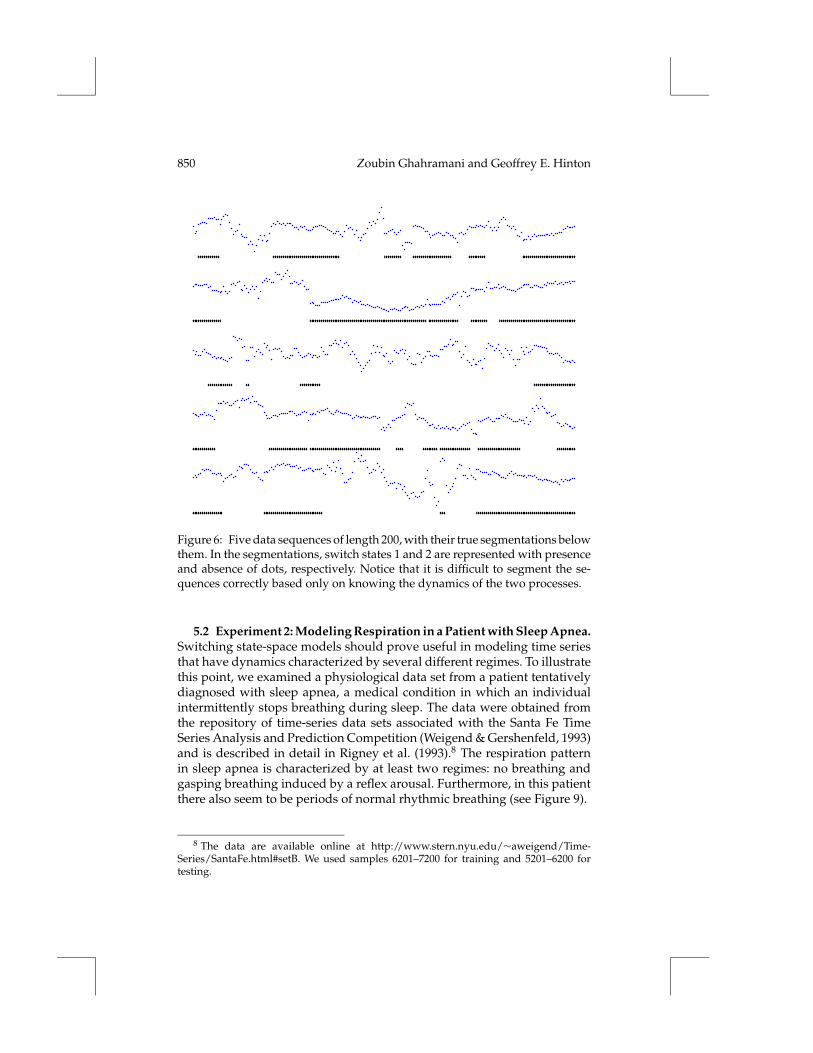
Figure 6: Five data sequences of length 200, with their true segmentations belowthem. In the segmentations, switch states 1 and 2 are represented with presenceand absence of dots, respectively. Notice that it is difficult to segment the se-quences correctly based only on knowing the dynamics of the two processes.

5.2 Experiment 2: Modeling Respiration in a Patient with Sleep Apnea.Switching state-space models should prove useful in modeling time seriesthat have dynamics characterized by several different regimes. To illustratethis point, we examined a physiological data set from a patient tentativelydiagnosed with sleep apnea, a medical condition in which an individualintermittently stops breathing during sleep. The data were obtained fromthe repository of time-series data sets associated with the Santa Fe TimeSeries Analysis and Prediction Competition (Weigend & Gershenfeld, 1993)and is described in detail in Rigney et al. (1993).8 The respiration patternin sleep apnea is characterized by at least two regimes: no breathing andgasping breathing induced by a reflex arousal. Furthermore, in this patientthere also seem to be periods of normal rhythmic breathing (see Figure 9).

8 The data are available online at http://www.stern.nyu.edu/∼aweigend/Time-Series/SantaFe.html#setB. We used samples 6201–7200 for training and 5201–6200 fortesting.


NAMT

NAMT

NAMT

NAMT

NAMT

NAMT

NAMT

NAMT

NAMT

NAMT

NAMT

NAMT

NAMT

NAMT

NAMT

NAMT

NAMT

NAMT

NAMT

NAMT

Figure 7: For 10 different sequences of length 200, segmentations are shownwith presence and absence of dots corresponding to the two SSMs generatingthese data. The rows are the segmentations found using the variational methodwith no annealing (N), the variational method with deterministic annealing(A), the gaussian merging method (M), and the true segmentation (T). All threeinference algorithms give real-valued h(m)t ; hard segmentations were obtainedby thresholding the final h(m)t values at 0.5. The first five sequences are the onesshown in Figure 6.


0 10 20 30 40 50 60 70 80 90 1000

20

40

60a

0 10 20 30 40 50 60 70 80 90 1000

10

20

30b

0 10 20 30 40 50 60 70 80 90 1000

10

20

30c

0 10 20 30 40 50 60 70 80 90 1000

10

20

30d

Percent Correct Segmentation

Figure 8: Histograms of percentage correct segmentations: (a) control, usingrandom segmentation; (b) variational inference without annealing; (c) varia-tional inference with annealing; (d) gaussian merging. Percentage correct seg-mentation was computed by counting the number of time steps for which thetrue and estimated segmentations agree.

We trained switching SSMs varying the random seed, the number ofcomponents in the mixture (M = 2 to 5), and the dimensionality of thestate-space in each component (K = 1 to 10) on a data set consisting of1000 consecutive measurements of the chest volume. As controls, we alsotrained simple SSMs (i.e., M = 1), varying the dimension of the state-spacefrom K = 1 to 10, and simple HMMs (i.e., K = 0), varying the number ofdiscrete hidden states from M = 2 to M = 50. Simulations were run untilconvergence or for 200 iterations, whichever came first; convergence wasassessed by measuring the change in likelihood (or bound on the likelihood)over consecutive steps of EM.

The likelihood of the simple SSMs and the HMMs was calculated on atest set consisting of 1000 consecutive measurements of the chest volume.For the switching SSMs, the likelihood is intractable, so we calculated thelower bound on the likelihood, B. The simple SSMs modeled the data verypoorly for K = 1, and the performance was flat for values of K = 2 to 10 (see


0 50 100 150 200 250 300 350 400 450 5005

0

5

10

15

20

time (s)

resp

iratio

na

0 50 100 150 200 250 300 350 400 450 5005

0

5

10

15

20

time (s)

resp

iratio

n

b

Figure 9: Chest volume (respiration force) of a patient with sleep apnea duringtwo noncontinuous time segments of the same night (measurements sampledat 2 Hz). (a) Training data. Apnea is characterized by extended periods of smallvariability in chest volume, followed by bursts (gasping). Here we see such be-havior around t = 250, followed by normal rhythmic breathing. (b) Test data. Inthis segment we find several instances of apnea and an approximately rhythmicregion. (The thick lines at the bottom of each plot are explained in the main text.)

Figure 10a). The large majority of runs of the switching state-space modelresulted in models with higher likelihood than those of the simple SMMs(see Figures 10b–10e). One consistent exception should be noted: for valuesof M = 2 and K = 6 to 10, the switching SSM performed almost identicallyto the simple SSM. Exploratory experiments suggest that in these cases,a single component takes responsibility for all the data, so the model hasM = 1 effectively. This may be a local minimum problem or a result ofpoor initialization heuristics. Looking at the learning curves for simple andswitching SSMs, it is easy to see that there are plateaus at the solutions foundby the simple one-component SSMs that the switching SSM can get caughtin (see Figure 11).

The likelihoods for HMMs with around M = 15 were comparable tothose of the best switching SSMs (see Figure 10f). Purely in terms of cod-


1 2 3 4 6 8 10

1.1

1

0.9

0.8SSM

K

a

1 2 3 4 6 8 10

1.1

1

0.9

0.8SwSSM (M=2)

K

b

1 2 3 4 6 8 10

1.1

1

0.9

0.8SwSSM (M=3)

K

c

1 2 3 4 6 8 10

1.1

1

0.9

0.8SwSSM (M=4)

K

d

1 2 3 4 6 8 10

1.1

1

0.9

0.8SwSSM (M=5)

K

e

0 10 20 30 40 50

1.1

1

0.9

0.8HMM

M

f

Figure 10: Log likelihood (nats per observation) on the test data from a total ofalmost 400 runs of simple state-space models (a), switching state-space modelswith differing numbers of components (b–e), and hidden Markov models (f).

ing efficiency, switching SSMs have little advantage over HMMs on thisdata.

However, it is useful to contrast the solutions learned by HMMs withthe solutions learned by the switching SSMs. The thick dots at the bot-tom of the Figures 9a and 9b show the responsibility assigned to one oftwo components in a fairly typical switching SSM with M = 2 compo-nents of state size K = 2. This component has clearly specialized to mod-eling the data during periods of apnea, while the other component modelsthe gasps and periods of rhythmic breathing. These two switching com-ponents provide a much more intuitive model of the data than the 10to 20 discrete components needed in an HMM with comparable codingefficiency.9

9 By using further assumptions to constrain the model, such as continuity of the real-valued hidden state at switch times, it should be possible to obtain even better performanceon these data.


0 50 100 150 200 2501.8

1.7

1.6

1.5

1.4

1.3

1.2

1.1

1

0.9

0.8

iterations of EM

log

P

Figure 11: Learning curves for a state space model (K = 4) and a switchingstate-space model (M = 2,K = 2).

6 Discussion

The main conclusion we can draw from the first series of experiments is thateven when given the correct model parameters, the problem of segmentinga switching time series into its components is difficult. There are combina-torially many alternatives to be considered, and the energy surface suffersfrom many local minima, so local optimization approaches like the varia-tional method we used are limited by the quality of the initial conditions.Deterministic annealing can be thought of as a sophisticated initializationprocedure for the hidden states: the final solution at each temperature pro-vides the initial conditions at the next. We found that annealing substantiallyimproved the quality of the segmentations found.

The first experiment also indicates that the much simpler gaussian merg-ing method performs comparably to annealed variational inference. Thegaussian merging methods have the advantage that at each time step, thecost function minimized has no local minima. This may account for howwell they perform relative to the nonannealed variational method. On theother hand, the variational methods have the advantage that they iterativelyimprove their approximation to the posterior, and they define a lower bound


on the likelihood. Our results suggest that it may be very fruitful to use thegaussian merging method to initialize the variational inference procedure.Furthermore, it is possible to derive variational approximations for otherswitching models described in the literature, and a combination of gaus-sian merging and variational approximation may provide a fast and robustmethod for learning and inference in those models.

The second series of experiments suggests that on a real data set believedto have switching dynamics, the switching SSM can indeed uncover mul-tiple regimes. When it captures these regimes, it generalizes to the test setmuch better than the simple linear dynamical model. Similar coding effi-ciency can be obtained by using HMMs, which due to the discrete nature ofthe state-space, can model nonlinear dynamics. However, in doing so, theHMMs had to use 10 to 20 discrete states, which makes their solutions lessinterpretable.

Variational approximations provide a powerful tool for inference andlearning in complex probabilistic models. We have seen that when appliedto the switching SSM, they can incorporate within a single framework well-known exact inference methods like Kalman smoothing and the forward-backward algorithm. Variational methods can be applied to many of theother classes of intractable switching models described in section 2.3. How-ever, training more complex models also makes apparent the importance ofgood methods for model selection and initialization.

To summarize, switching SSMs are a dynamical generalization of mix-ture-of-experts neural networks, are closely related to well-known mod-els in econometrics and control, and combine the representations underly-ing HMMs and linear dynamical systems. For domains in which we havesome a priori belief that there are multiple, approximately linear dynami-cal regimes, switching SSMs provide a natural modeling tool. Variationalapproximations provide a method to overcome the most difficult problemin learning switching SSMs: that the inference step is intractable. Determin-istic annealing further improves on the solutions found by the variationalmethod.

Appendix A: Notation

Symbol Size Description

Variables

Yt D× 1 observation vector at time t{Yt} D× T sequence of observation vectors [Y1,Y2, . . .YT]X(m)

t K × 1 state vector of state-space model (SSM) m at time tXt KM× 1 entire real-valued hidden state at time t: Xt =

[X(1)t , . . . ,X(M)

t ]


St M× 1 switch state variable (represented either as dis-crete variable St ∈ {1, . . .M}, or as an M×1 vectorSt = [S(1)t , . . .S(M)

t ]′ where S(m)t ∈ {0, 1})

Model parameters

A(m) K × K state dynamics matrix for SSM mC(m) D× K output matrix for SSM mQ(m) K × K state noise covariance matrix for SSM mµ(m)X1

K × 1 initial state mean for SSM mQ(m)1 K × K initial state noise covariance matrix for SSM mR D×D output noise covariance matrixπ M× 1 initial state probabilities for switch state8 M×M state transition matrix for switch state

Variational parameters

h(m)t 1× 1 responsibility of SSM m for Yt

q(m)t 1× 1 related to expected squared error if SSM m gen-erated Yt

Miscellaneous

X′ matrix transpose of X|X| matrix determinant of X〈X〉 expected value of X under the Q distribution

Dimensions

D size of observation vectorT length of a sequence of observation vectorsM number of state-space modelsK size of state vector in each state-space model

Appendix B: Derivation of the Variational Fixed-Point Equations

In this appendix we derive the variational fixed-point equations used in thelearning algorithm for switching SSMs. First, we write out the probabilitydensity P defined by a switching SSM. For convenience, we express thisprobability density in the log domain, through its associated energy func-tion or hamiltonian, H. The probability density is related to the hamiltonianthrough the usual Boltzmann distribution (at a temperature of 1),

P(·) = 1Z

exp{−H(·)},


where Z is a normalization constant required such that P(·) integrates tounity. Expressing the probabilities in the log domain does not affect the re-sulting algorithm. We then similarly express the approximating distributionQ through its hamiltonian HQ. Finally, we obtain the variational fixed-pointequations by setting to zero the derivatives of the KL divergence betweenQ and P with respect to the variational parameters of Q.

The joint probability of observations and hidden states in a switchingSSM is (see equation 3.1)

P({St,Xt,Yt}) =[

P(S1)

T∏t=2

P(St|St−1)

]M∏

m=1

[P(

X(m)1

) T∏t=2

P(

X(m)t |X(m)

t−1

)]

·T∏

t=1

P(Yt|Xt,St). (B.1)

We proceed to dissect this expression into its constituent parts. The initialprobability of the switch variable at time t = 1 is given by

P(S1) =M∏

m=1

(π(m)

)S(m)1, (B.2)

where S1 is represented by an M×1 vector [S(1)1 . . .S(M)

1 ] where S(m)1 = 1 if theswitch state is in state m, and 0 otherwise. The probability of transitioningfrom a switch state at time t− 1 to a switch state at time t is given by

P(St|St−1) =M∏

m=1

M∏n=1

(8(m,n)

)S(m)t S(n)t−1. (B.3)

The initial distribution for the hidden state variable in SSM m is gaussianwith mean µ(m)X1

and covariance matrixQ(m)1 :

P(

X(m)1

)=∣∣∣2πQ(m)1

∣∣∣− 12

exp{−1

2

(X(m)

1 − µ(m)X1

)′ (Q(m)1

)−1 (X(m)

1 − µ(m)X1

)}. (B.4)

The probability distribution of the state in SSM m at time t given the stateat time t− 1 is gaussian with mean A(m)X(m)

t−1 and covariance matrixQ(m):

P(

X(m)t |X(m)

t−1

)=∣∣∣2πQ(m)∣∣∣− 1

2 exp{−1

2

(X(m)

t − A(m)X(m)t−1

)′(Q(m))−1

·(

X(m)t − A(m)X(m)

t−1

)}. (B.5)


Finally, using equation 3.2, we can write:

P(Yt|Xt,St) =M∏

m=1

[|2πR|− 1

2

exp{−1

2

(Yt − C(m)X(m)

t

)′R−1

(Yt − C(m)X(m)

t

)}]S(m)t

(B.6)

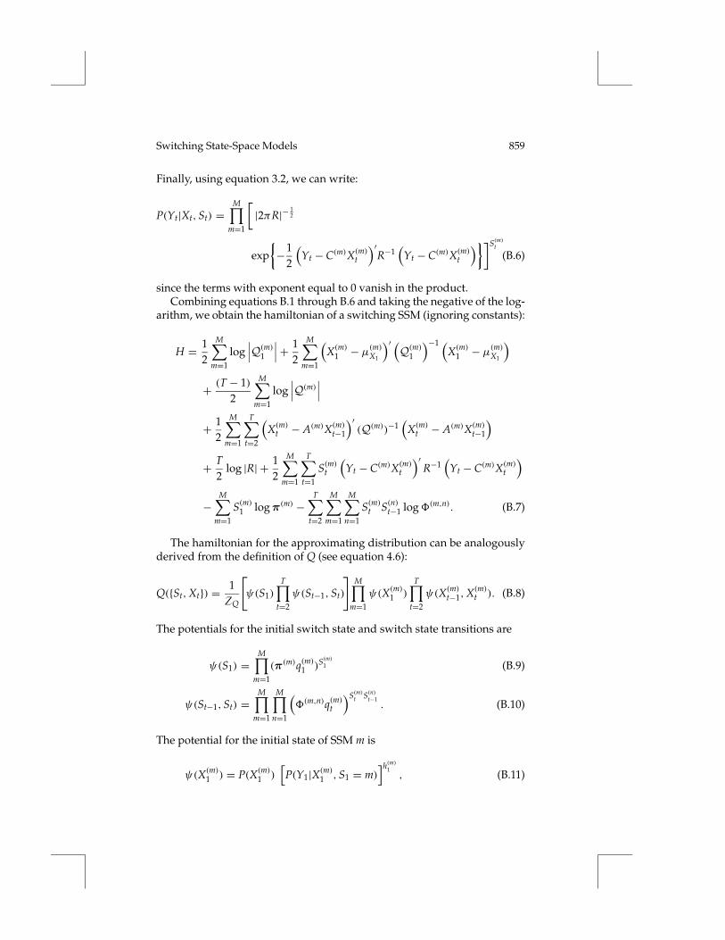
since the terms with exponent equal to 0 vanish in the product.Combining equations B.1 through B.6 and taking the negative of the log-

arithm, we obtain the hamiltonian of a switching SSM (ignoring constants):

H = 12

M∑m=1

log∣∣∣Q(m)1

∣∣∣+ 12

M∑m=1

(X(m)

1 − µ(m)X1

)′ (Q(m)1

)−1 (X(m)

1 − µ(m)X1

)+ (T − 1)

2

M∑m=1

log∣∣∣Q(m)∣∣∣

+ 12

M∑m=1

T∑t=2

(X(m)

t − A(m)X(m)t−1

)′(Q(m))−1

(X(m)

t − A(m)X(m)t−1

)+ T

2log |R| + 1

2

M∑m=1

T∑t=1

S(m)t

(Yt − C(m)X(m)

t

)′R−1

(Yt − C(m)X(m)

t

)−

M∑m=1

S(m)1 logπ(m) −T∑

t=2

M∑m=1

M∑n=1

S(m)t S(n)t−1 log8(m,n). (B.7)

The hamiltonian for the approximating distribution can be analogouslyderived from the definition of Q (see equation 4.6):

Q({St,Xt}) = 1ZQ

[ψ(S1)

T∏t=2

ψ(St−1,St)

]M∏

m=1

ψ(X(m)1 )

T∏t=2

ψ(X(m)t−1,X(m)

t ). (B.8)

The potentials for the initial switch state and switch state transitions are

ψ(S1) =M∏

m=1

(π(m)q(m)1 )S(m)1 (B.9)

ψ(St−1,St) =M∏

m=1

M∏n=1

(8(m,n)q(m)t

)S(m)t S(n)t−1. (B.10)

The potential for the initial state of SSM m is

ψ(X(m)1 ) = P(X(m)

1 )[P(Y1|X(m)

1 ,S1 = m)]h(m)1

, (B.11)


and the potential for the state at time t given the state at time t− 1 is

ψ(X(m)t−1,X(m)

t ) = P(X(m)t |X(m)

t−1)[P(Yt|X(m)

t ,St = m)]h(m)t

. (B.12)

The hamiltonian for Q is obtained by combining these terms and takingthe negative logarithm:

HQ = 12

M∑m=1

log |Q(m)1 | +12

M∑m=1

(X(m)

1 − µ(m)X1

)′(Q(m)1 )−1

(X(m)

1 − µ(m)X1

)+ (T − 1)

2

M∑m=1

log |Q(m)|

+ 12

M∑m=1

T∑t=2

(X(m)

t − A(m)X(m)t−1

)′(Q(m))−1

(X(m)

t − A(m)X(m)t−1

)+ T

2

M∑m=1

log |R|+ 12

M∑m=1

T∑t=1

h(m)t

(Yt−C(m)X(m)

t

)′R−1

(Yt−C(m)X(m)

t

)−

M∑m=1

S(m)1 logπ(m) −T∑

t=2

M∑m=1

M∑n=1

S(m)t S(n)t−1 log8(m,n)

−T∑

t=1

M∑m=1

S(m)t log q(m)t . (B.13)

Comparing HQ with H, we see that the interaction between the S(m)t andthe X(m)

t variables has been eliminated, while introducing two sets of varia-tional parameters: the responsibilities h(m)t and the bias terms on the discreteMarkov chain, q(m)t . In order to obtain the approximation Q that maximizesthe lower bound on the log-likelihood, we minimize the KL divergenceKL(Q‖P) as a function of these variational parameters:

KL(Q‖P) =∑{St}

∫Q({St,Xt}) log

Q({St,Xt})P({St,Xt}|{Yt})d{Xt} (B.14)

= 〈H −HQ〉 − log ZQ + log Z, (B.15)

where 〈·〉 denotes expectation over the approximating distribution Q andZQ is the normalization constant for Q. Both Q and P define distributions inthe exponential family. As a consequence, the zeros of the derivatives of KLwith respect to the variational parameters can be obtained simply by equat-ing derivatives of 〈H〉 and 〈HQ〉 with respect to corresponding sufficientstatistics (Ghahramani, 1997):

∂〈HQ −H〉∂〈S(m)t 〉

= 0 (B.16)


∂〈HQ −H〉∂〈X(m)

t 〉= 0 (B.17)

∂〈HQ −H〉∂〈P(m)t 〉

= 0 (B.18)

where P(m)t = 〈X(m)t X(m)

t′〉 − 〈X(m)

t 〉〈X(m)t 〉′ is the covariance of X(m)

t under Q.Many terms cancel when we subtract the two hamiltonians,

HQ −H =M∑

m=1

T∑t=1

12

(h(m)t − S(m)t

) (Yt − C(m)X(m)

t

)′R−1

·(

Yt − C(m)X(m)t

)− S(m)t log q(m)t . (B.19)

Taking derivatives, we obtain

∂〈HQ −H〉∂〈S(m)t 〉

= − log q(m)t −12

⟨(Yt − C(m)X(m)

t

)′R−1

(Yt − C(m)X(m)

t

)⟩(B.20)

∂〈HQ −H〉∂〈X(m)

t 〉= −

(h(m)t − 〈S(m)t 〉

) ((Yt − C(m)〈X(m)

t 〉)′R−1C(m))

(B.21)

∂〈HQ −H〉∂P(m)t

= 12

(h(m)t − 〈S(m)t 〉

) (C(m)

′R−1C(m)

)(B.22)

From equation B.20, we get the fixed-point equation, 4.12, for q(m)t . Bothequations B.21 and B.22 are satisfied when h(m)t = 〈S(m)t 〉. Using the fact that〈S(m)t 〉 = Q(St = m) we get equation 4.11.

References

Ackerson, G. A., & Fu, K. S. (1970). On state estimation in switching environ-ments. IEEE Transactions on Automatic Control, AC-15(1):10–17.

Anderson, B. D. O., & Moore, J. B. (1979). Optimal filtering. Englewood Cliffs, NJ:Prentice-Hall.

Athaide, C. R. (1995). Likelihood evaluation and state estimation for nonlinear statespace models. Unpublished doctoral dissertation, University of Pennsylvania.

Baldi, P., Chauvin, Y., Hunkapiller, T., & McClure, M. (1994). Hidden Markovmodels of biological primary sequence information. Proc. Nat. Acad. Sci.(USA), 91(3), 1059–1063.

Bar-Shalom, Y., & Li, X.-R. (1993). Estimation and tracking. Boston: Artech House.Baum, L., Petrie, T., Soules, G., & Weiss, N. (1970). A maximization technique oc-

curring in the statistical analysis of probabilistic functions of Markov chains.Annals of Mathematical Statistics, 41, 164–171.


Bengio, Y., & Frasconi, P. (1995). An input-output HMM architecture. InG. Tesauro, D. S. Touretzky, & T. K. Leen (Eds.), Advances in neural informationprocessing systems, 7 (pp. 427–434). Cambridge, MA: MIT Press.

Cacciatore, T. W., & Nowlan, S. J. (1994). Mixtures of controllers for jump linearand non-linear plants. In J. D. Cowan, G. Tesauro, & J. Alspector (Eds.),Advances in neural information processing systems, 6 (pp. 719–726). San Mateo:Morgan Kaufmann Publishers.

Carter, C. K., & Kohn, R. (1994). On Gibbs sampling for state space models.Biometrika, 81, 541–553.

Chaer, W. S., Bishop, R. H., & Ghosh, J. (1997). A mixture-of-experts frameworkfor adaptive Kalman filtering. IEEE Trans. on Systems, Man and Cybernetics.

Chang, C. B., & Athans, M. (1978). State estimation for discrete systems withswitching parameters. IEEE Transactions on Aerospace and Electronic Systems,AES-14(3), 418–424.

Cover, T., & Thomas, J. (1991). Elements of information theory. New York: Wiley.Dean, T., & Kanazawa, K. (1989). A model for reasoning about persistence and

causation. Computational Intelligence, 5(3), 142–150.Dempster, A., Laird, N., & Rubin, D. (1977). Maximum likelihood from in-

complete data via the EM algorithm. J. Royal Statistical Society Series B,39, 1–38.

Deng, L. (1993). A stochastic model of speech incorporating hierarchical non-stationarity. IEEE Trans. on Speech and Audio Processing, 1(4), 471–474.

Digalakis, V., Rohlicek, J. R., & Ostendorf, M. (1993). ML estimation of a stochas-tic linear system with the EM algorithm and its application to speech recog-nition. IEEE Transactions on Speech and Audio Processing, 1(4), 431–442.

Elliott, R. J., Aggoun, L., & Moore, J. B. (1995). Hidden Markov models: Estimationand control. New York: Springer-Verlag.

Fraser, A. M., & Dimitriadis, A. (1993). Forecasting probability densities by usinghidden Markov models with mixed states. In A. S. Wiegand & N. A. Gershen-feld (Eds.), Time series prediction: Forecasting the future and understanding thepast (pp. 265–282). Reading, MA: Addison-Wesley.

Ghahramani, Z. (1997). On structured variational approximations (Tech. Rep.No. CRG-TR-97-1). Toronto: Department of Computer Science, Universityof Toronto. Available online at: http://www.gatsby.ucl.ac.uk/∼zoubin/papers/struct.ps.gz.

Ghahramani, Z., & Hinton, G. E. (1996a). Parameter estimation for linear dynam-ical systems (Tech. Rep. No. CRG-TR-96-2). Toronto: Department of Com-puter Science, University of Toronto. Available online at: http://www.gatsby.ucl.ac.uk/∼zoubin/papers/tr-96-2.ps.gz.

Ghahramani, Z., & Hinton, G. E. (1996b). The EM algorithm for mixtures of fac-tor analyzers (Tech. Rep. No. CRG-TR-96-1). Toronto: Department of Com-puter Science, University of Toronto. Available online at: http://www.gatsby.ucl.ac.uk/∼zoubin/papers/tr-96-1.ps.gz.

Ghahramani, Z., & Jordan, M. I. (1997). Factorial hidden Markov models. Ma-chine Learning, 29, 245–273.

Goodwin, G., & Sin, K. (1984). Adaptive filtering prediction and control. EnglewoodCliffs, NJ: Prentice-Hall.


Hamilton, J. D. (1989). A new approach to the economic analysis of nonstationarytime series and the business cycle. Econometrica, 57, 357–384.

Hamilton, J. D. (1994). Time series analysis. Princeton, NJ: Princeton UniversityPress.

Harrison, P. J., & Stevens, C. F. (1976). Bayesian forecasting (with discussion). J.Royal Statistical Society B, 38, 205–247.

Hinton, G. E., Dayan, P., & Revow, M. (1997). Modeling the manifolds of imagesof handwritten digits. IEEE Transactions on Neural Networks, 8, 65–74.

Jacobs, R. A., Jordan, M. I., Nowlan, S. J., & Hinton, G. E. (1991). Adaptivemixture of local experts. Neural Computation, 3, 79–87.

Jordan, M. I., Ghahramani, Z., Jaakkola, T. S., & Saul, L. K. (1998). An intro-duction to variational methods in graphical models. In M. I. Jordan (Ed.),Learning in graphical models. Norwell, MA: Kluwer.

Jordan, M. I., & Jacobs, R. (1994). Hierarchical mixtures of experts and the EMalgorithm. Neural Computation, 6, 181–214.

Juang, B. H., & Rabiner, L. R. (1991). Hidden Markov models for speech recog-nition. Technometrics, 33, 251–272.

Kadirkamanathan, V., & Kadirkamanathan, M. (1996). Recursive estimation ofdynamic modular RBF networks. In D. Touretzky, M. Mozer, and M. Has-selmo (Eds.), Advances in neural information processing systems, 8 (pp. 239–245).Cambridge, MA: MIT Press.

Kalman, R. E., & Bucy, R. S. (1961). New results in linear filtering and prediction.Journal of Basic Engineering (ASME), 83D, 95–108.

Kanazawa, K., Koller, D., & Russell, S. J. (1995). Stochastic simulation algorithmsfor dynamic probabilistic networks. In P. Besnard & S. Hanks (Eds.), Uncer-tainty in artificial intelligence. Proceedings of the Eleventh Conference (pp. 346–351). San Mateo, CA: Morgan Kaufmann.

Kehagias, A., & Petrides, V. (1997). Time series segmentation using predictivemodular neural networks. Neural Computation, 9(8), 1691–1710.

Kim, C.-J. (1994). Dynamic linear models with Markov-switching. J. Economet-rics, 60, 1–22.

Lauritzen, S. L., & Spiegelhalter, D. J. (1988). Local computations with probabil-ities on graphical structures and their application to expert systems. J. RoyalStatistical Society B, 157–224.

Ljung, L., & Soderstrom, T. (1983). Theory and practice of recursive identification.Cambridge, MA: MIT Press.

Meila, M., & Jordan, M. I. (1996). Learning fine motion by Markov mixtures ofexperts. In D. S. Touretzky, M. C. Mozer, & M. E. Hasselmo (Eds.), Advancesin neural information processing systems, 8. Cambridge, MA: MIT Press.

Neal, R. M., & Hinton, G. E. (1998). A new view of the EM algorithm that justifiesincremental, sparse, and other variants. In M. I. Jordan (Ed.), Learning ingraphical models. Norwell, MA: Kluwer.

Parisi, G. (1988). Statistical field theory. Redwood City, CA: Addison-Wesley.Pawelzik, K., Kohlmorgen, J., & Muller, K.-R. (1996). Annealed competition of

experts for a segmentation and classification of switching dynamics. NeuralComputation, 8(2), 340–356.


Pearl, J. (1988). Probabilistic reasoning in intelligent systems: Networks of plausibleinference. San Mateo, CA: Morgan Kaufmann.

Rabiner, L. R., & Juang, B. H. (1986). An introduction to hidden Markov models.IEEE Acoustics, Speech & Signal Processing Magazine, 3, 4–16.

Rauch, H. E. (1963). Solutions to the linear smoothing problem. IEEE Transactionson Automatic Control, 8, 371–372.

Rigney, D., Goldberger, A., Ocasio, W., Ichimaru, Y., Moody, G., & Mark, R.(1993). Multi-channel physiological data: Description and analysis. In A.Weigend & N. Gershenfeld (Eds.), Time series prediction: Forecasting the futureand understanding the past (pp. 105–129). Reading, MA: Addison-Wesley.

Roweis, S., & Ghahramani, Z. (1999). A unifying review of linear gaussian mod-els. Neural Computation, 11(2), 305–345.

Saul, L. and Jordan, M. I. (1996). Exploiting tractable substructures in intractablenetworks. In D. Touretzky, M. Mozer, & M. Hasselmo (Eds.), Advances inneural information processing systems, 8. Cambridge, MA: MIT Press.

Shumway, R. H., & Stoffer, D. S. (1982). An approach to time series smoothingand forecasting using the EM algorithm. J. Time Series Analysis, 3(4), 253–264.

Shumway, R. H., & Stoffer, D. S. (1991). Dynamic linear models with switching.J. Amer. Stat. Assoc., 86, 763–769.

Smyth, P. (1994). Hidden Markov models for fault detection in dynamic systems.Pattern Recognition, 27(1), 149–164.

Smyth, P., Heckerman, D., & Jordan, M. I. (1997). Probabilistic independencenetworks for hidden Markov probability models. Neural Computation, 9, 227–269.

Ueda, N., & Nakano, R. (1995). Deterministic annealing variant of the EM algo-rithm. In G. Tesauro, D. Touretzky, & J. Alspector (Eds.), Advances in neuralinformation processing systems, 7 (pp. 545–552). San Mateo, CA: Morgan Kauf-mann.

Weigend, A., & Gershenfeld, N. (1993). Time series prediction: Forecasting the futureand understanding the past. Reading, MA: Addison-Wesley.

Received March 2, 1998; accepted March 16, 1999.

variational learning for switching state-space …mlg.eng.cam.ac.uk/pub/pdf/ghahin00a.pdfswitching...

Documents