Conservation Genetics1: 115–133, 2000.© 2000Kluwer Academic Publishers. Printed in the Netherlands.

115

Variability and differentiation of microsatellites in the genus Dasyurusandconservation implications for the large Australian carnivorous marsupials

Karen B. Firestone1,2,∗, Bronwyn A. Houlden1,2, William B. Sherwin2 & Eli Geffen3

1Conservation Research Center, Taronga Zoo, P.O. Box 20, Mosman NSW 2088, Australia;2School of BiologicalScience, University of New South Wales, NSW 2052, Australia;3Institute for Nature Conservation Research, TelAviv University, Ramat Aviv 69978, Israel (∗Corresponding author: E-mail: K.Firestone@unsw.edu.au)

Received 16 November 1999; accepted 8 March 2000

Key words:carnivorous marsupials, conservation units,Dasyurus, ESUs, genetic differentiation, genetic variability,microsatellites, MUs

Abstract

All four species of Australian quolls (Dasyurusspecies) have declined since European settlement in terms of bothrange and population numbers. Six highly polymorphic simple sequence repeats (CAn microsatellites) were usedto estimate the genetic variability and population differentiation within and among twenty populations (includingmuseum specimens from six populations), as a preliminary means of assessing population conservation status andrelative levels of variability within members of the genus. Overall mean expected heterozygosity (HE) and correctedallelic diversity (A′) were highest among western quolls. Northern quolls, eastern quolls, and tiger quolls werenot significantly different from each other in either measure. There were also significant differences in diversityamong populations within species. Genetic differentiation was estimated by a number of methods and showedthat the microsatellites used here were useful for defining differences both among species and populations. Allelefrequency data were summarised by two-dimensional MDS, which was able to partition populations into distinctspecies clusters. Similarly, the assignment test was able to assign most individuals to both the correct species andpopulation levels. Results of MDS and the assignment test may prove useful in forensic applications. Geneticdistance and subdivision between pairs of populations were assessed by two means based on different mutationmodels for microsatellites: infinite alleles model (Nei’s D, FST) and stepwise mutation model (Goldstein’sδµ2,RST). Pairwise measures of population subdivision indicate that most populations should be conserved as separatemanagement units. We discuss results of these analyses in terms of applications to conservation for each of the fourAustralian species of quoll and provide a genetic basis for future population monitoring in these species.

Introduction

Genetic variability or diversity has long been recog-nized as a key component of population and conser-vation genetics. The loss of genetic variation (eitherallelic diversity or heterozygosity), due to drift,inbreeding, or other factors can reduce both individualfitness and the ability of populations to adapt to alteredenvironmental conditions (Lacy 1997). Inbreedingmay cause decreased levels of heterozygosity in indi-viduals. Inbreeding depression, as a result of closeconsanguineous matings, may decrease individualfitness via a number of routes (Gall 1987; Ralls et

al. 1988; Frankham 1995; Newman and Pilson 1997).The long term viability of populations also may bethreatened by the loss of genetic variation due to drift.Loss of variability may affect small populations bydecreasing the ability to adapt to changing environ-ments and by increasing the probability of extinctiondue to stochastic effects (Lacy 1997). Alternatively,relatively high levels of genetic diversity may increasequalities associated with fitness (Allendorf and Leary1986).

Differentiation between both species and popula-tions is another area of concern to conservationists, asthis gives an indication of the evolutionary divergence

116

between taxa. For conservation purposes, it is vital toensure that the species in question are indeed differentenough that we can easily distinguish between themgenetically. There are many examples now in the liter-ature where taxa that are morphologically different aregenetically similar and vice versa (e.g. Firestone et al.1999). Also, lack of genetic differentiation betweenmorphologically distinct species may indicate that theprocess of hybridization is occurring (e.g. Roy et al.1994).

At the population level much debate has beenfocussed on determining what units to conserve,particularly given limited resources (Vane-Wright etal. 1991; Crozier 1992; Rojas 1992; Vogler andDeSalle 1994; Waples 1998). Moritz (1994) andMoritz et al. (1995) suggested that populations that aregenetically divergent at both nuclear and mitochon-drial loci should be conserved as separate units, i.e.evolutionarily significant units (ESUs) or managementunits (MUs). Several recent studies have applied theseconcepts to conservation of endangered taxa (e.g. Popeet al. 1996; Zhu et al. 1998; Firestone et al. 1999).

Analysis of microsatellites has become animportant tool in population studies and is usefulfor estimating both variability and differentiation(e.g. Taylor et al. 1994; FitzSimmons et al. 1995;García-Moreno et al. 1996; Houlden et al. 1996;Brunner et al. 1998). Microsatellites are single-locus,biparentally inherited, and highly variable markersoccurring throughout the genome (Tautz 1989).They contain short-length (usually di-, tri-, or tetra-nucleotide) repeat units which vary in the number ofrepeats between individuals (Tautz and Renz 1984;Tautz 1989). In addition, microsatellites have provento be highly informative where other markers haveyielded little information when applied to the samespecies (e.g. Paetkau and Strobeck 1994; Estoup et al.1998; Goodman 1998).

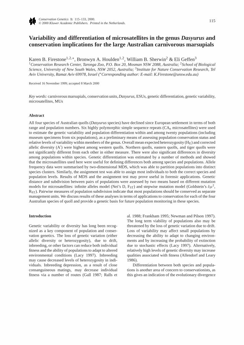
The six species of quolls (Dasyurusspp.) areamong the largest of the remaining carnivorousmarsupials in Australia and Papua New Guinea. Thefour species of quolls found in Australia range in sizefrom seven kilograms (some male tiger quolls) to lessthan 400 g (female northern quolls) (Strahan 1998).Like their placental counterparts, these large marsupialcarnivores have faced declines in numbers and distri-bution throughout their ranges (Figure 1). The reasonsfor these declines are poorly understood, and are likelyto be due to a number of interacting factors. Factorssuch as habitat loss, the introduction of feral predatorsand poisonous prey resources, altered fire regimes,

disease susceptibility, and continued persecution byhumans may all have played different roles in thedecline of each species (Maxwell et al. 1996).

Each quoll species is considered to be threatenedto some degree and each species has had a differenthistory of decline. The western quoll (Dasyurusgeoffroii) exhibited a population decline on a contin-ental scale and survives only in one area of south-western Western Australia (WA). Due to recentsuccessful management efforts, this species has beendowngraded from ‘endangered’ to ‘vulnerable’ bythe World Conservation Union (IUCN) (Serena et al.1991; Orell and Morris 1994; Maxwell et al. 1996).Eastern quoll (D. viverrinus) numbers were decimatedaround the turn of this century; they are currentlypresumed extinct on the mainland. This speciespersists in Tasmania, however, where populationnumbers are stable. Eastern quolls are currently desig-nated as ‘lower risk-near threatened’ (IUCN listing;Maxwell et al. 1996). The decline of northern quolls(D. hallucatus) is a relatively recent phenomenon.Once widely distributed throughout the northern thirdof the continent, this species is now restricted tosix main population centres (Braithwaite and Griffiths1994) and is also currently designated as ‘lowerrisk-near threatened’ by the IUCN. The southernmainland subspecies of tiger quolls (D. maculatusmaculatus) declined early this century, however unlikeeastern quolls, tiger quolls persisted on the main-land where populations are scattered and numbersare low (Mansergh 1984). Tiger quolls also occurin Tasmania, where populations are thought to benaturally limited by competition from both Tasmaniandevils (Sarcophilus harrisii) and eastern quolls (Jones1995). Southern mainland tiger quolls are presentlyrestricted to less than 50% of their range and are listedas ‘vulnerable’ by the IUCN. The northern mainlandsubspecies of tiger quoll (D. m. gracilis) is centredin a few small localities in north Queensland andis currently considered ‘endangered’ by the IUCN(Maxwell et al. 1996). Despite these widespread andprecipitous declines, little attention has been given togenetic implications for conservation management ofthese taxa.

The applications of genetic management to quollconservation are multifaceted. Captive managementand breeding of western quolls is part of this speciesrecovery plan and has been successful for a numberof years (Orell and Morris 1994), yet determinationof the level of diversity of the captive population hasnot been attempted. This is important in light of the

117

Figure 1. Current (black) and past (grey + black) distribution of the Australian quolls including sample sites. (A)Dasyurus maculatus, (B) D.viverrinus, (C) D. hallucatus, (D) D. geoffroii. A, B, and D redrawn from Strahan (1998); C redrawn from Braithwaite and Griffiths (1994).See Table 1 for key to population names.

reintroduction program taking place as part of thisspecies recovery plan. In addition, there are plans toreintroduce eastern quolls into areas of their formerrange on the mainland; it is important to evalu-ate the genetic variation and differentiation betweendifferent stocks before reintroducing animals to areaswhere remnant populations might persist. Withoutsound knowledge of the genetic diversity withinand between the remaining Tasmanian populationsof eastern quolls, it is difficult to determine whichpopulations are valuable sources for reintroductions.Analysis of the mitochondrial DNA control region andmicrosatellites has proven to be very useful in eluci-dating conservation units among tiger quolls (Fire-stone et al. 1999) and may be so for northern quolls.

We undertook this study to determine the relativelevels of variability and differentiation present bothamong species and among populations within species,to provide baseline information regarding variabilitywithin populations of each species for future popula-tion monitoring, and to assist wildlife agencies andmanagers in making sound conservation decisionsregarding these species. In particular, we test thefollowing null hypotheses: (1) genetic diversity is thesame among all populations within each species, (2)each species of quoll has the same genetic diversity,(3) there is no genetic differentiation between popula-tions within each species, and (4) there is nogenetic differentiation between species of quolls. Weexamined six highly polymorphic (CA)n microsatellite

118

markers and a total of 347 individuals, representing 20populations and four species, as a means of assessingthe genetic variability and differentiation in quollsand as a basis for future population monitoring andconservation breeding programs.

Methods

Study populations, DNA samples, and populationscreening

Tissue samples were collected from all Australianspecies of quolls representing 20 different populations(Figure 1, Table 1). Six of these sample populations(PE, AR, NE, ST, GL, and WY) were from driedskins held in museum collections; two populations(BF, GI) were from captive stock bred in captivity fora number of years; and four groups (TE, TT, NE, andBT) were from samples collected opportunisticallyand represent sites encompassing broader geographicareas. Samples were either fresh tissues (skin, blood,liver, or muscle) from live-trapped or road-killed indi-viduals, or dried preserved skins from museum speci-mens. DNA from fresh tissues was extracted accordingto standard protocols by phenol-chloroform extractionfollowed by ethanol precipitation (Sambrook et al.1989). DNA from museum specimens was extractedby a modified guanidine thiocyanate method (Boom etal. 1990; Hoss and Pääbo 1993). The microsatellitemarkers were derived from either a tiger quoll or amixed tiger/eastern quoll genetic library. The isolationof these markers and amplification procedures used inthis study have been described elsewhere (Firestone1999).

Aliquots of the PCR products were mixed with anequal volume of formamide loading dye, heated to80◦C, and loaded on a 6% polyacrylamide sequencinggel containing 50% w/v urea. Gels were fixed (10%glacial acetic acid/10% methanol) and dried, thenexposed to autoradiographic film (X-OMAT, Kodakor Hyperfilm-HP, Amersham). Alleles were scoredby comparison with a size marker (M13 sequence,USB) electrophoresed alongside the samples on eachsequencing gel. Eighteen populations were typed at allsix loci; ST was typed at four loci while AR was typedat five loci.

Statistical analyses

Deviations from Hardy-Weinberg equilibrium (HWE)were tested in each population by one of two methods

as implemented in GENEPOP (Raymond and Rousset1995): either complete enumeration for loci with upto four alleles (Louis and Dempster 1987) or by aMarkov chain method for loci with five or more alleles(Guo and Thompson 1992). Genetic variability ofspecies and populations was measured as the numberof alleles per locus (A) and unbiased expected hetero-zygosity (HE) for each locus using BIOSYS (Swoffordand Selander 1981). Differences in mean HE betweenspecies and populations were tested by analysis ofvariance (ANOVA; Sokal and Rohlf 1981) and posthoc hypotheses were examined using Scheffe’s test.Empirical studies have shown that population sizeand level of genetic variability are positively corre-lated (Frankham 1996). Similarly, measures of geneticdiversity are likely to be affected by small sample size(e.g. Roy et al. 1994); A more so than HE (Nei et al.1975; Bouzat et al. 1998). Sample sizes in this studyranged from three to 58 individuals per population,therefore, we could not discount the effects of limitedsampling regimes in assessing allelic diversity. Tocompare the number of alleles in species that differedin sample size, we calculated the expected number ofalleles in an infinite population by Monte-Carlo simu-lations (Roy et al. 1994). We selected individuals atrandom without replacement and calculated the cumu-lative number of alleles until all individuals had beensampled. This procedure was repeated 1000 times foreach species and the mean and standard deviation ofthe number of alleles was calculated as a function ofsample size. A quasi-Newton best fit curve was thenapplied to the means using the equation y =αx/(x +β) where y = number of alleles, and x = number ofindividuals. In this equationα and β are constants,whereα represents the number of alleles in an infinitepopulation. In addition, we employed residual analysisas a measure of corrected allelic diversity (A′) usingANOVA and Scheffe’s post hoc tests, to examine inter-specific and interpopulation differences in number ofalleles. The data were log-transformed prior to theanalysis to accommodate nonlinearity and deviationfrom the normal distribution. To control for the effectof sample size, we have used residuals generated bylinear regression of sample size versus number ofalleles.

Genetic differentiation was assessed by a numberof methods. First, the number of unique or privatealleles found between populations or species may beseen as a measure of genetic differentiation; howeversimilarly to the number of alleles, the number ofunique alleles is also affected by the extent of the

119

Table 1. Species and populations sampled

Map reference

Species Location Pop East South Status N A

Tiger quoll 1. Mount Windsor, Qld MW 145◦02′ 16◦15′ Wild 12 2.5 (0.2)

Dasyurus maculatus 2. Glenn Innis, NSW GI 152◦04′ 29◦44′ Captive 5 2.7 (0.4)

3. Copeland, NSW CO 151◦48′ 31◦59′ Wild 9 4.3 (0.5)

4. Chichester State Forest, NSW CH 151◦31′ 32◦08′ Wild 12 4.7 (0.6)

5. Barrington Guest House, NSW BG 151◦42′ 32◦09′ Wild 16 4.7 (0.5)

6. Barrington Tops area, NSW BT Wide area Wild 11 4.2 (0.9)

7. Badja State Forest, NSW BS 149◦33′ 36◦07′ Wild 6 2.5 (0.3)

8. Suggan Buggan, Vic SB 148◦22′ 36◦57′ Wild 3 2.5 (0.2)

9. Wynyard, Tas WY 145◦44′ 41◦00′ Museum 32 4.3 (1.1)

10. Central Tasmania TT Wide area Wild 11 3.8 (0.6)

Eastern quoll 11. New South Wales NE Wide area Museum 25 7.0 (1.4)

Dasyurus viverrinus 12. Studley Park, Vic ST 145◦01′ 37◦48′ Museum 13 2.8 (0.5)∗13. Gladstone, Tas GL 148◦01′ 40◦58′ Museum 58 4.8 (0.8)

14. Vale of Belvoir, Tas VB 145◦53′ 41◦32′ Wild 21 3.5 (0.8)

15. Central Tasmania TE Wide area Wild 14 3.7 (0.6)

Northern quoll 16. Kakadu National Park, NT KA 132◦12′ 12◦44′ Wild 26 9.0 (1.7)

Dasyurus hallucatus 17. Archer River, Qld AR 142◦09′ 13◦35′ Museum 9 3.6 (0.7)§

18. Atherton Tableland, Qld AT 145◦35′ 17◦03′ Wild 6 4.0 (1.0)

Western quoll 19. Perth area, WA PE 116◦10′ 32◦12′ Museum 23 8.8 (0.8)

Dasyurus geoffroii 20. Batalling State Forest, WA BF 116◦13′ 33◦14′ Captive 35 9.2 (0.7)

N = number of individuals sampled per population; A = mean uncorrected allelic diversity, standard errors in parentheses.∗Fourloci analysed.§Five loci analysed. All other populations typed at all six loci.

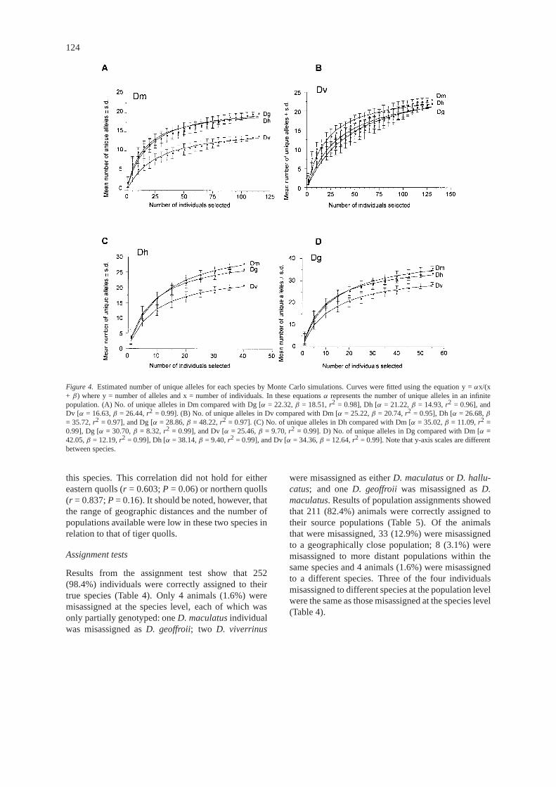
sampling regime. When closely related species arecompared, the number of unique alleles found withineach species is a measure of genetic distinction.However, this is strongly influenced by the samplesize and geographic scope of the sampling withineach taxon. We calculated the expected number ofunique alleles for each species in comparison withanother species, given different sample sizes, usingMonte-Carlo simulations as above.

Second, we summarized allele frequencies forpopulations into two dimensions using multidimen-sional scaling (MDS), which makes few assump-tions of the structure of the data. MDS analysis wasperformed using a convergence factor of 0.005 and50 iterations as implemented in STATISTICA (Stat-soft, Inc.). Finally, genetic distances and popula-tion subdivision among all pairwise comparisons ofpopulations were estimated using methods based onboth the step-wise mutations model (SMM) and theinfinite alleles model (IAM), since neither mutationmodel is strictly correct for microsatellites (Primmeret al. 1998). Thus we employed Goldstein’sδµ2

distance (SMM) (Goldstein et al. 1995) and Nei’sunbiased genetic distance (Nei’s D; IAM) (Nei 1972).Subdivision among populations was estimated by bothRST (SMM) (Slatkin 1995; Goodman 1997) and FST(IAM) (Wright 1951), since RST includes allele sizeinformation while FST is based only on genetic drift. AMantel procedure was used to test for correlation bothbetweenδµ2 and D and between RST and FST. Nei’sD was further used to construct a neighbor-joiningtree as implemented in the NEIGHBOR program inPHYLIP (Felsenstein 1995). Bootstrap analysis wasdone by first generating 1000 distance matrices usingMICROSAT (Minch et al. 1998); 1000 bootstrappedneighbor-joining trees were then constructed usingthe NEIGHBOR program and summarized by theCONSENSE program in PHYLIP (Felsenstein 1995).Significance of all pairwise FST values was assessedby 10,000 iterations as implemented in FSTAT (v.2.8) not assuming HWE (Goudet 1999). Furthermore,Mantel tests were performed to assess the relationshipof genetic differentiation between populations (FST) tothat of geographic distance.

120

Lastly, an assignment test (available fromwww.biology.ualberta.ca/jbrzusto/Doh.html) wasperformed to determine how characteristic anindividual’s genotype was of both the species andpopulation from which it was sampled (Paetkau et al.1995; Paetkau et al. 1998). The expected frequencyof each individuals’ genotype was calculated at boththe species and population levels and assigned tothe species or population for which the expectedfrequency was greatest. All frequencies were adjustedto avoid zeros using the method of Titterington et al.(1981).

Results

Genetic variability of microsatellites in quolls

The six microsatellite loci used in this study werehighly polymorphic in all species examined, with14–23 total different alleles per locus (Appendix A).Uncorrected mean A per population ranged from 2.5(MW, BS, and SB, tiger quolls) to 9.2 (BF, westernquolls) and mean HE ranged from 0.469 (BS, tigerquolls) to 0.883 (PE, western quolls). The samplesanalysed in both GI and WY populations were mono-morphic at a single locus each (locus 1.3 and 3.3.1,respectively); the samples analysed from the ATpopulation were monomorphic at two loci, 1.3 and4.4.10. Allele frequency distributions were highlyskewed at each locus, generally with two or threecommon alleles and many rare alleles.

Deviations from Hardy Weinberg equilibrium

Some loci deviated from HWE proportions in elevenof the twenty populations. All six loci in the BFpopulation deviated from HWE. Deviations were alsofound in three loci from NE (1.3, 3.1.2, 4.4.2), andGL (3.1.2, 3.3.1, 3.3.2) populations; two loci fromeach of TE (3.3.2, 4.4.2), KA (3.1.2, 3.3.2) and PE(1.3, 3.3.1) populations; and one locus from each ofthe MW (1.3), BS (3.1.2), WY (4.4.2), ST (3.3.1),and VB (3.3.2) populations. No locus was prevalentin deviations from HWE.

We also examined overall HW proportions,combined over all loci, for each population. Of alltiger quoll populations, only one (WY) was signifi-cantly deviant from overall HWE at all six loci (χ2 =24.2, P = 0.007); this was due to a general hetero-zygote deficiency. Among eastern quoll populationsNE, ST, GL and VB were all significantly different

from genotype proportions expected under HWE, overall loci. Significant deviation of GL (χ2 infinity, Phighly significant) was due to heterozygote excessesat two loci (3.3.1, 3.3.2) and heterozygote deficitsat one locus (3.1.2). All other significant differencesin eastern quolls were due to heterozygote deficits(NE, χ2 infinity, P highly significant; ST,χ2 = 19.9,P = 0.0029; VB,χ2 = 28.2, P = 0.0052). Amongnorthern quolls, KA was the only population signifi-cantly different from overall HWE proportions (χ2 =35.3, P = 0.0004); this deviation was due to hetero-zygote deficits. In addition, neither western quollpopulation was in HWE proportions. Overall differ-ences from HWE in the BF and PE populations (BF,χ2 = 78.2, P < 0.0001; PE,χ2 infinity, P highlysignificant) were due to heterozygote deficiencies.

Genetic diversity among species

Monte Carlo simulations of the estimated cumulativealleles for each species are shown in Figure 2. Thecumulative number of alleles begins to asymptotebetween 10–20 samples for most species except forD.viverrinus, which begins to asymptote after approxi-mately 25 individuals are sampled. These simulationsindicate that our sampling regime was adequate inpicking up a substantial proportion of alleles presentfor most populations, although in populations whereonly a few individuals were sampled the number ofalleles is underestimated.

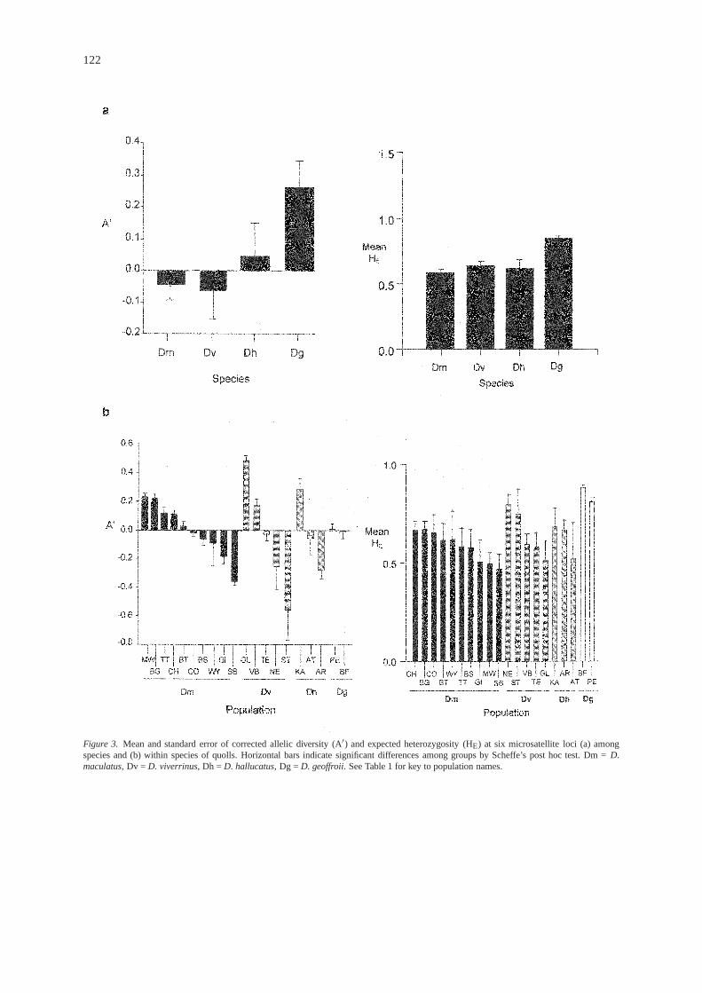
Uncorrected allelic diversity (A) is shown in Table1. In general, western quolls had higher numbers ofalleles than any other species, while tiger quolls hadlower allelic diversity than other species. Measuresof genetic diversity after correction for sample sizedifferences are shown in Figure 3. Significant differ-ences were found among species in both correctedallelic diversity (A′; ANOVA F = 10.59;P≤ 0.0001 )and mean HE (ANOVA F = 5.70,P = 0.001) (Figure3a). Post hoc tests revealed that HE was signifi-cantly higher in populations of western quolls than inany other species; western quolls also had a signifi-cantly higher allelic diversity than either tiger quollsor eastern quolls, but were not significantly differentto northern quolls. Eastern, tiger, and northern quollswere not significantly different from each other ineither A′ or mean HE.

Genetic diversity among populations within species

When each species was examined separately, signifi-cant differences in A′ were found among popula-

121

Figure 2. Estimated cumulative number of alleles per sample size for each species by Monte Carlo simulation. Curves were fitted using theequation y =α x/(x + β) where y = number of alleles and x = number of individuals. In these equationsα represents the number of alleles in aninfinite population. (A)D. maculatus, α = 57.0,β = 10.87,r2 = 0.979; (B)D. viverrinus, α = 69.70,β = 20.88,r2 = 0.965; (C)D. hallucatus,α = 76.11,β = 9.54,r2 = 0.999; (D)D. geoffroii, α = 80.23,β = 10.61,r2 = 0.993. Note that y-axis scales are different between species.

tions of all species except western quolls (Figure 3b).Among tiger quoll populations, GI and SB had signifi-cantly lower A′ than MW, BG, TT, CH, and BT(ANOVA F = 9.83, P < 0.0001). Among easternquoll populations, GL had significantly higher allelicdiversity than TE, NE, and ST; furthermore, ST hadsignificantly lower allelic diversity than GL, VB, andTE (ANOVA F = 14.18,P< 0.0001). Among northernquoll populations, KA had a significantly highernumber of alleles than either AR or AT (ANOVAF =11.01,P< 0.001). There were no differences in allelicdiversity between the two western quoll populations(unpairedt-test,t = 0.31;P = 0.76).

Significant differences in levels of HE also werefound among eastern quoll populations (ANOVAF

= 2.88, P = 0.045) and western quoll populations(ANOVA F = 8.77, P = 0.014), however post hoctests of eastern quolls indicated that there were nosignificant pairwise differences. Among western quollpopulations, PE had significantly higher HE than BF(Figure 3b).

Genetic differentiation among species: unique alleles

Each species possessed only a subset of the totalalleles found in the genus (Appendix A). While therewas great overlap among species in the alleles present(e.g. alleles 101–107 were found in all four species atlocus 3.3.1), there was also substantial partitioning ateach locus (e.g. at locus 3.3.1, alleles 91, 93, 97, and

122

Figure 3. Mean and standard error of corrected allelic diversity (A′) and expected heterozygosity (HE) at six microsatellite loci (a) amongspecies and (b) within species of quolls. Horizontal bars indicate significant differences among groups by Scheffe’s post hoc test. Dm =D.maculatus, Dv = D. viverrinus, Dh = D. hallucatus, Dg = D. geoffroii. See Table 1 for key to population names.

123

Table 2. The number and percentage (in parenthesis) of uniquealleles between four species of quolls

Dm Dv Dh Dg

Dm (54) – 14 (25.9) 20 (37.0) 20 (37.0)

Dv (63) 23 (36.5) – 22 (34.9) 22 (34.9)

Dh (62) 28 (45.2) 21 (33.9) – 26 (41.9)

Dg (70) 36 (51.4) 29 (41.4) 34 (48.6) –

Total number of alleles in each species is in parenthesis besidethe species name at the left column of the table. All 20 popula-tions were included.

117 were unique to northern quolls, whereas alleles127–145 were found only in western quolls). Theeffect of our sampling regime on the number of uniquealleles observed among species was examined andthe proportion of unique alleles estimated by MonteCarlo simulations is shown in Figure 4 and Table 2. IngeneralD. geoffroiihad the highest number of uniquealleles in relation to all other species, whereasD.maculatushad the lowest number of unique allelesin relation to all other species. After approximately30–40 individuals of most species had been sampledthe graphs begin to asymptote (e.g. Figure 4a, c, d)indicating that the proportion of unique alleles foundin relation to other species has peaked.D. viverrinus,however, may require additional samples to reach thisasymptote (Figure 4b).

Genetic differentiation among species: allelefrequencies

Genetic differentiation was also examined using allelefrequency data. The differences in allele frequen-cies among species and populations of quolls weresummarized using MDS (Figure 5) which showed thatpopulations within species generally clustered closelyin two-dimensional space. Furthermore, these data fitin two dimensions with low stress (0.10) and with ahigh proportion of the variance accounted for (r2 =0.94), indicating a good fit of the data in multidimen-sional space.

Genetic differentiation among populations withinspecies: population subdivision

Pairwise genetic differentiation measures amongpopulations were also estimated by both FST and RST.A Mantel test showed that FST and RST values werehighly correlated (r = 0.72;P≤ 0.001); therefore onlyFST values are shown in Table 3. All pairwise compar-isons of FST values were tested for significance. Most

pairwise comparisons showed significant populationsubdivision both between populations and betweenspecies (Table 3). An exception was found amongpopulations of tiger quolls, particularly among the fourpopulations from the Barrington area. None of thesepairs of populations showed significant subdivision.Additionally, the SB population was not differentiatedfrom most other populations, but this is probably dueto the very low sample size for this population.

Genetic differentiation among populations withinspecies: genetic distance measures

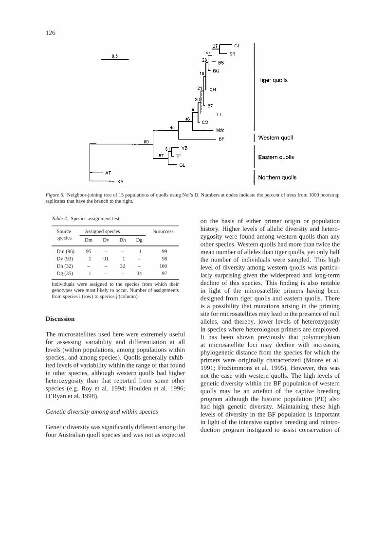
A Mantel test of Nei’s D and Goldstein’sδµ2 indi-cated that these distance measures were significantlycorrelated (r = 0.64;P≤ 0.001). We therefore presentpairwise values of Nei’s D only (Table 3). Exami-nation of both genetic distances among tiger quollpopulations revealed that MW was consistently themost distant from all other tiger quoll populations.Lowest genetic distances were found among the fourgeographically close populations of tiger quolls (CO,CH, BG, BT) by Nei’s D; the results forδµ2 were notconsistent with Nei’s D, however (data not shown).Among eastern quolls, both Nei’s D andδµ2 valuesindicated that the Tasmanian populations (GL, VB,TE) were closer to each other than to the mainlandpopulations (NE and ST; data not shown). Nei’s D alsoshowed that the two northern quoll populations (KAand AT) were more closely related to each other thaneither was to any other population.

Nei’s D was used to build a neighbour joining treeamong 15 populations of quolls (Figure 6). These datashow that all species form their own clades, althoughbootstrap support is very low in many cases. Similarto trees based on mtDNA sequences, northern quollpopulations are the most distant from other popula-tions based on microsatellites and thus form an earlysplit. The topology of this tree, however, is notconsistent with those based on mitochondrial DNAloci (Krajewski et al. 1997; Firestone, in press).

Geographic distance vs. FST

The relationship of genetic subdivision (FST) togeographic distance was examined by a Mantel testwithin each of the three species in which more thantwo populations were available. There was a signifi-cant correlation between geographic distance and FSTfor tiger quoll populations (r = 0.615;P = 0.01), indi-cating that distance explains a substantial amount ofthe genetic variance observed between populations of

124

Figure 4. Estimated number of unique alleles for each species by Monte Carlo simulations. Curves were fitted using the equation y =αx/(x+ β) where y = number of alleles and x = number of individuals. In these equationsα represents the number of unique alleles in an infinitepopulation. (A) No. of unique alleles in Dm compared with Dg [α = 22.32,β = 18.51,r2 = 0.98], Dh [α = 21.22,β = 14.93,r2 = 0.96], andDv [α = 16.63,β = 26.44,r2 = 0.99]. (B) No. of unique alleles in Dv compared with Dm [α = 25.22,β = 20.74,r2 = 0.95], Dh [α = 26.68,β= 35.72,r2 = 0.97], and Dg [α = 28.86,β = 48.22,r2 = 0.97]. (C) No. of unique alleles in Dh compared with Dm [α = 35.02,β = 11.09,r2 =0.99], Dg [α = 30.70,β = 8.32,r2 = 0.99], and Dv [α = 25.46,β = 9.70,r2 = 0.99]. D) No. of unique alleles in Dg compared with Dm [α =42.05,β = 12.19,r2 = 0.99], Dh [α = 38.14,β = 9.40,r2 = 0.99], and Dv [α = 34.36,β = 12.64,r2 = 0.99]. Note that y-axis scales are differentbetween species.

this species. This correlation did not hold for eithereastern quolls (r = 0.603;P = 0.06) or northern quolls(r = 0.837;P = 0.16). It should be noted, however, thatthe range of geographic distances and the number ofpopulations available were low in these two species inrelation to that of tiger quolls.

Assignment tests

Results from the assignment test show that 252(98.4%) individuals were correctly assigned to theirtrue species (Table 4). Only 4 animals (1.6%) weremisassigned at the species level, each of which wasonly partially genotyped: oneD. maculatusindividualwas misassigned asD. geoffroii; two D. viverrinus

were misassigned as eitherD. maculatusor D. hallu-catus; and oneD. geoffroii was misassigned asD.maculatus. Results of population assignments showedthat 211 (82.4%) animals were correctly assigned totheir source populations (Table 5). Of the animalsthat were misassigned, 33 (12.9%) were misassignedto a geographically close population; 8 (3.1%) weremisassigned to more distant populations within thesame species and 4 animals (1.6%) were misassignedto a different species. Three of the four individualsmisassigned to different species at the population levelwere the same as those misassigned at the species level(Table 4).

125

Figure 5. MDS based upon Euclidean distances among 15 populations of quolls. ( ) D. maculatus, (+) D. viverrinus, (�) D. hallucatus, (N)D. geoffroii. Stress = 0.10, Rsq = 0.94.

Table 3. Pairwise comparison of Nei’s D (below the diagonal) and FST (above the diagonal)

Species/population

DM DV DH DGMW GI CO CH BG BT BS SB TT GL VB TE KA AT BF

Tiger quoll

MW – 0.445∗ 0.156∗ 0.221∗ 0.221∗ 0.275∗ 0.399∗ 0.429∗ 0.304∗ 0.451∗ 0.385∗ 0.389∗ 0.378∗ 0.486∗ 0.242∗GI 1.59 – 0.242 0.183∗ 0.169∗ 0.218∗ 0.310 0.207 0.327∗ 0.377∗ 0.342∗ 0.351∗ 0.361∗ 0.472 0.256∗CO 0.27 0.64 – 0.011 0.047 0.000 0.167∗ 0.184∗ 0.125∗ 0.393∗ 0.327∗ 0.322∗ 0.313∗ 0.385∗ 0.161∗CH 0.48 0.42 0.03 – 0.029 0.019 0.117∗ 0.136 0.156∗ 0.376∗ 0.319∗ 0.312∗ 0.309∗ 0.374∗ 0.174∗BG 0.51 0.39 0.11 0.07 – 0.058 0.143∗ 0.086 0.156∗ 0.356∗ 0.307∗ 0.299∗ 0.299∗ 0.370∗ 0.185∗BT 0.64 0.46 0.01 0.03 0.12 – 0.124∗ 0.110 0.128∗ 0.393∗ 0.332∗ 0.331∗ 0.323∗ 0.394∗ 0.196∗BS 1.01 0.60 0.32 0.20 0.27 0.20 – 0.117 0.257∗ 0.441∗ 0.390∗ 0.396∗ 0.370∗ 0.462 0.272∗SB 1.76 0.36 0.50 0.33 0.20 0.23 0.16 – 0.222 0.411∗ 0.347∗ 0.356 0.329∗ 0.432 0.250∗TT 0.69 0.97 0.25 0.36 0.38 0.26 0.53 0.54 – 0.416∗ 0.350∗ 0.349∗ 0.340∗ 0.425∗ 0.221∗

Eastern quoll

GL 1.80 0.97 1.66 1.51 1.31 1.52 1.54 1.46 1.71 – 0.222∗ 0.109∗ 0.384∗ 0.440∗ 0.329∗VB 1.50 1.19 1.63 1.57 1.44 1.55 1.64 1.59 1.56 0.41 – 0.078∗ 0.323∗ 0.385∗ 0.273∗TE 1.40 1.17 1.46 1.39 1.29 1.43 1.53 1.56 1.43 0.14 0.15 – 0.329∗ 0.399∗ 0.269∗

Northern quollKA 2.83 3.08 3.00 2.99 2.47 2.88 2.69 2.83 2.91 2.12 2.03 2.12 – 0.223∗ 0.225∗AT 3.53 2.92 2.54 2.48 2.65 2.28 1.98 2.38 2.93 1.76 1.82 1.90 0.67∗ – 0.266∗

Western quollBF 1.04 1.65 0.81 0.97 1.11 1.05 1.65 2.73 1.20 2.21 2.51 2.28 2.08 1.93 –

Shaded areas denote major groups. Asterisks indicate significant differentiation between pairs of populations after Bonferroni correctionfor multiple comparisons.

126

Figure 6. Neighbor-joining tree of 15 populations of quolls using Nei’s D. Numbers at nodes indicate the percent of trees from 1000 bootstrapreplicates that have the branch to the right.

Table 4. Species assignment test

Source Assigned species % successspecies Dm Dv Dh Dg

Dm (96) 95 – – 1 99

Dv (93) 1 91 1 – 98

Dh (32) – – 32 – 100

Dg (35) 1 – – 34 97

Individuals were assigned to the species from which theirgenotypes were most likely to occur. Number of assignmentsfrom species i (row) to species j (column).

Discussion

The microsatellites used here were extremely usefulfor assessing variability and differentiation at alllevels (within populations, among populations withinspecies, and among species). Quolls generally exhib-ited levels of variability within the range of that foundin other species, although western quolls had higherheterozygosity than that reported from some otherspecies (e.g. Roy et al. 1994; Houlden et al. 1996;O’Ryan et al. 1998).

Genetic diversity among and within species

Genetic diversity was significantly different among thefour Australian quoll species and was not as expected

on the basis of either primer origin or populationhistory. Higher levels of allelic diversity and hetero-zygosity were found among western quolls than anyother species. Western quolls had more than twice themean number of alleles than tiger quolls, yet only halfthe number of individuals were sampled. This highlevel of diversity among western quolls was particu-larly surprising given the widespread and long-termdecline of this species. This finding is also notablein light of the microsatellite primers having beendesigned from tiger quolls and eastern quolls. Thereis a possibility that mutations arising in the primingsite for microsatellites may lead to the presence of nullalleles, and thereby, lower levels of heterozygosityin species where heterologous primers are employed.It has been shown previously that polymorphismat microsatellite loci may decline with increasingphylogenetic distance from the species for which theprimers were originally characterized (Moore et al.1991; FitzSimmons et al. 1995). However, this wasnot the case with western quolls. The high levels ofgenetic diversity within the BF population of westernquolls may be an artefact of the captive breedingprogram although the historic population (PE) alsohad high genetic diversity. Maintaining these highlevels of diversity in the BF population is importantin light of the intensive captive breeding and reintro-duction program instigated to assist conservation of

127

Table 5. Population assignment test for 15 populations of quolls

Assigned population

Source Dm Dv Dh Dgpop MW GI CO CH BG BT BS SB TT GL VB TE KA AT BF % success

MW (12) 12 – – – – – – – – – – – – – – 100

GI (5) – 4 – 1 – – – – – – – – – – – 80

CO (9) – – 1 4 1 3 – – – – – – – – – 11

CH (17) – – 1 13 2 1 – – – – – – – – – 76

BG (22) – – 2 3 15 1 – 1 – – – – – – – 68

BT (11) – – 4 1 – 3 – – 2 – – – – – 1 27

BS (6) – – 1 – – – 5 – – – – – – – – 83

SB (3) – – – – – 1 – 2 – – – – – – – 75

TT (11) – – 1 – – – – – 10 – – – – – – 91

GL (58) – – – – – – 1 – – 53 – 4 – – – 91

VB (21) – – – – – – – – – – 20 1 – – – 95

TE (14) – – – – – – – – – 3 2 9 – – – 64

KA (26) – – – – – – – – – – – – 26 – – 100

AT (6) – – – – – – – – – – – – 1 5 – 83

BF (35) – – 1 – 1 – – – – – – – – – 33 94

Individuals were assigned to the populations from which their genotypes were most likely to occur. Number of assignments frompopulation i (row) to population j (column) are indicated. Shaded areas denote populations within species that are in close geographicproximity.

this species. In addition, high levels of microsatel-lite variability may be useful for tracking paternityand reproductive success within that colony. Northernquolls, tiger quolls and eastern quolls were not signifi-cantly different from one another in either measure ofdiversity, indicating that the same genetic processesmay be operating within these three species (i.e. drift,mutation, migration).

Differences in variability within species were alsoapparent and were as expected (i.e. low variation wasfound in small or isolated populations). The GI andSB populations of tiger quolls had lower correctedallelic diversity than that of either the MW, BG,TT, CH, or BT populations. Both the GI and SBpopulations are small: GI has been a captive bredcolony for approximately 18 years with little geneticexchange (Bruce Kubbere, pers. comm.) and the SBpopulation is from an area in Victoria where therehave been very few sightings or records over thelast decade. In contrast, the MW, BG, CH, and BTpopulations are wild populations with relatively highnumbers of individuals. Similarly, there were differ-ences in allelic diversity among populations of easternquolls and among populations of northern quolls.The mainland populations of eastern quolls (NE, ST)had significantly lower allelic diversity than popula-tions in Tasmania (GL, VB, TE). This result might

be surprising given that theory predicts low geneticdiversity among island populations when compared tomainland populations (Frankham 1997). Two possibleexplanations exist: lower levels of diversity may bean artefact of the difficulties in amplifying DNA frommuseum tissues, or the mainland populations mayhave been on the brink of extinction when thesesamples were collected. Within northern quolls, theKA population had higher allelic diversity than eitherAT or AR. Again, the KA population is in a relativelystable state, with large population numbers extendedover a wide area. It is thought that the AT populationis now isolated and in decline and the AR populationis extinct.

Genetic differentiation among and within species

Each species possessed some unique alleles (Table 2),which were useful in defining species clusters. Phylo-genetic analysis, based on distance values amongpopulations, (Nei’s D, Table 3; Figure 6) was able topartition species into distinct clades, although boot-strap support was limited. In phylogenetic reconstruc-tions based on genetic distances between mtDNAsequences, eastern and western quolls are sisterspecies (Krajewski et al. 1997; Firestone, in press);in the reconstruction based on distances between

128

microsatellite alleles, tiger and western quolls aresister species (Figure 6). Phylogenetic reconstructionsbased on microsatellites are less sensitive to sharedancestral polymorphisms than those based on mtDNAdue to the extremely high mutation rate of microsatel-lites and homoplasy of alleles (similarity in phenotype,but not identity by descent) (Estoup et al. 1995).Similarly, MDS analysis was able to partition popula-tions into species clusters based on the presence ofunique alleles and differences in allele frequencies(Figure 5). The positioning of populations into distinctspecies clusters or clades indicates that the microsatel-lites used here are potentially useful for identifyingdifferent species of quolls in forensic tests. The assign-ment test (Table 4) and analysis of the mitochondrialDNA control region (Firestone in press) also mayserve this function and may be even more useful whenindividuals are considered.

Most population pairs within species were signifi-cantly differentiated from one another based on allelefrequencies (pairwise FST values; Table 3). This indi-cates that most populations should be consideredas separate management units (MUs) according torecommendations by Moritz (1994). One notableexception is found among tiger quoll populations. Thefour populations from the Barrington Tops region (CO,CH, BG, BT) are all located within a radius of 50km, and were not significantly subdivided based onmicrosatellite loci; similarly, there were difficulties inassigning individuals correctly among these popula-tions (Table 5). However, studies of allele frequenciesof the mtDNA control region have shown that someof these populations are actually differentiated (Fire-stone et al. 1999). Another exception may be foundamong many of the pairwise comparisons of SB; thelack of genetic differentiation between SB and theseother populations may be due to the very small samplesize of this population; the same may hold true for theGI and AT populations (Table 3).

Conservation implications

Western quollsWestern quolls possessed greater allelic diversity andlevels of heterozygosity than the other species. Inaddition, western quolls also possessed the greatestnumber of unique alleles in relation to other species.The recovery plan for western quolls was begunin 1991 with the breeding colony consisting of 20captive founders (3 males, 5 females, and 12 youngfrom two litters) and additional wild caught young

used to augment the captive population (Serena etal. 1991). Supplemental wild-caught males havebeen periodically introduced to the captive colonyfor breeding purposes, and surplus young have beenroutinely released to one of several different unoccu-pied translocation sites (Serena et al. 1991; Orell andMorris 1994). Maintaining high levels of genetic vari-ability within the captive colony of western quollsis important to the long term viability of the trans-located wild populations. Current estimates of vari-ability in the extant population (BF) compared to aextinct population (PE) show no differences in themean number of alleles but higher levels of hetero-zygosity in the extant population. The high levels ofdiversity and heterozygosity in the BF population maybe a manifestation of non-random breeding, due toactive management of the captive population whereasthe high levels of heterozygosity in the PE popula-tion may be a manifestation of changing genotypicstructure over an extended sampling period.

Breeding programs may greatly influence thelevels of diversity within a captive population and theresults presented here could indicate that the captivebreeding program has been successful in maintaininghigh levels of diversity. Due to the success of therecovery program, including wide spread fox baiting,this species has been downgraded from ‘endangered’to ‘vulnerable’ by the IUCN. Continued geneticmonitoring of the captive and translocated populationsis recommended as a means of assessing inbreeding orfounder effects in recolonized areas.

Tiger quolls

Tiger quolls had low numbers of alleles in comparisonwith other species, however when this was correctedfor sample size, there was no significant differencebetween tiger, eastern, or northern quolls in levelsof HE or in A′, indicating that the same evolutionaryforces (drift, mutation, migration) may be operatingon these species.

Genetic subdivision shows that many populationsof tiger quolls are separate MUs for conservationpurposes (FST values; Table 3) although microsatellitedata did not show subdivision amongst the populationsfrom the Barrington Tops region (CH, CO, BG, BT).However, other studies have shown that the Barringtonregion populations are actually subdivided based onfrequency differences in mtDNA, which is likely dueto sex biased dispersal in these populations (Firestoneet al. 1999).

129

In addition, the MW population (ascribed toD.maculatus gracilis) has been shown to be part of themainland ESU, but the TT population forms a separateESU to that on the mainland (Firestone et al. 1999).The TT population should be managed as a separatetaxon to all other populations, whereas translocationsbetween different MUs belonging to the same ESUmay be advisable in cases where population numbershave dropped to low levels. However, analysis of FSTversus geographic distance was significant for thisspecies, indicating that distance itself explains muchof the genetic variance observed between populationsof tiger quolls. This implies that these animals arequite stationary, and dispersal distances are rathershort relative to the large distances between samplelocalities. For this reason alone, it is important not tomix populations by reintroducing individuals from onesite to another unless they are in close proximity.

Eastern quolls

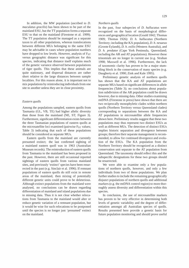
Among the populations sampled, eastern quolls fromTasmania (GL, VB, TE) had higher allelic diversitythan those from the mainland (NE, ST; Figure 3).Furthermore, significant differentiation exists betweenthe three Tasmanian populations of eastern quolls atthe microsatellite loci examined (pairwise FST values;Table 3) indicating that each of these populationsshould be considered as separate MUs.

Eastern quolls from the mainland are currentlypresumed extinct; the last confirmed sighting ofa mainland eastern quoll was in 1963 (AustralianMuseum records). The reintroduction of eastern quollsfrom Tasmania to the mainland has been proposed inthe past. However, there are still occasional reportedsightings of eastern quolls from various mainlandsites, and previously ‘extinct’ species have been resur-rected in the past (e.g. Sinclair et al. 1996). If remnantpopulations of eastern quolls do still exist in remoteareas of the mainland, then mixing of potentiallydifferent genetic units could prove to be deleterious.Although extinct populations from the mainland wereanalysed, no conclusions can be drawn regardingdifferentiation of mainland and island populations dueto missing data. Thus it is not clear whether reloca-tions from Tasmania to the mainland would alter orreduce genetic variation of a remnant population, butit would be wise for such relocations to be postponeduntil the species is no longer just ‘presumed’ extincton the mainland.

Northern quolls

In the past, four subspecies ofD. hallucatuswererecognized on the basis of morphological differ-ences and geographical location (Gould 1842; Thomas1909; Thomas 1926):D. h. hallucatus(NorthernTerritory; including the KA population),D. h. nesaeus(Groote Eylandt),D. h. exilis(Western Australia), andD. h. predator (Cape York Peninsula, Queensland;including the AR and AT populations). However thesetrinomials are no longer in current use (e.g. Strahan1998; Maxwell et al. 1996). Furthermore, the lackof taxonomic clarity has proven to be a major stum-bling block in the conservation of many species (e.g.Daugherty et al. 1990; Zink and Kale 1995).

Preliminary genetic analysis of northern quollshas shown that the KA and AT populations areseparate MUs based on significant differences in allelefrequencies (Table 3); no conclusions about popula-tion subdivision of the AR population could be drawnhowever, due to missing data. Other studies examiningmtDNA (Firestone in press) have shown that there aretwo reciprocally monophyletic clades within northernquolls (Northern Territory versus Queensland clades)corresponding to separations between the KA andAT populations in microsatellite allele frequenciesshown here. Preliminary results suggest that these twopopulations may thus represent two distinct ESUs aswell as different MUs. The detection of distinct ESUsimplies historic separation and divergence betweengroups; therefore their separate management is recom-mended, to allow for continued divergence and evolu-tion of the ESUs. The KA population from theNorthern Territory should be recognized as a distinctconservation unit separate to the AT population fromQueensland. The taxonomy should reflect this and thesubspecific designations for these two groups shouldbe resurrected.

We were able to examine only a few popula-tions of northern quolls, however, and only a fewindividuals from two of those populations. We planfurther studies to include the remaining geographicallydisjunct populations of northern quolls and additionalmarkers (e.g. the mtDNA control region) to more thor-oughly assess diversity and differentiation within thisspecies.

In conclusion, the use of microsatellite markershas proven to be very effective in determining bothlevels of genetic variability and the degree of differ-entiation amongst all Australian species of quolls.Results presented here provide a genetic basis forfuture population monitoring and should prove useful

130

to conservation managers and agencies in decisionmaking processes related to the conservation of thesespecies.

Acknowledgements

The authors thank the many people and institutionswho kindly helped collect samples used in this study:C. Belcher, S. Burnett, J. Byron, N. Cooper, F. Craven,R. Darr, R. Dickens, J. Dixon, B. Dowling, L. Frigo,C. Gallagher, L. Gibson, J. Giles, J. Griffiths, G.Hall, M. Jones, A. Kelly, B. Lewis, D. Longbottom,L. Leung, K. Morris, D. Moyle, M. Murray, M.Oakwood, M. Pennay, L. Pope, S. Priestly, J. Rain-bird, B. Read, J. Seebeck, J. Titmarsh, L. Vogelnest,B. Walker, The Australian Museum, The WesternAustralian Museum, The Museum of Victoria, theQueen Victoria Museum, Featherdale Wildlife Park,Trowunna Wildlife Park, Perth Zoo, and Taronga Zoo.We also thank State Forests of New South Wales, theNSW National Parks and Wildlife Service, the owners,managers and staff of Barrington Guest House andW. Greville who provided assistance in many ways.Thanks also go to C. Dickman, J. Giles, M. Roy, A.Kremer, and two anonymous reviewers for providingcomments that improved this paper. KF receivedfunding for this work from an Australian PostgraduateResearch Award, the Estate of W.V. Scott, BarringtonGuest House, and the Zoological Parks Board of NewSouth Wales.

References

Allendorf FW, Leary RF (1986) Heterozygosity and fitness innatural populations of animals. In:Conservation Biology: TheScience of Scarcity and Diversity(ed. Soulé ME), pp. 57–76.Sinauer Associates, Sunderland, MA.

Boom R, Sol CJA, Salimans MMM, Jansen CL, Wertheim-vanDillen PME, Van der Noordaa J (1990) Rapid and simple methodfor purification of nucleic acids.Journal of Clinical Microbio-logy, 28, 495–503.

Bouzat JL, Cheng HH, Lewin HA, Westemeier RL, Brawn JD, PaigeKN (1998) Genetic evaluation of a demographic bottleneck in thegreater prairie chicken.Cons. Biol., 12, 836–843.

Braithwaite RW, Griffiths AD (1994) Demographic variation andrange contraction in the northern quoll,Dasyurus hallucatus(Marsupialia: Dasyuridae).Wildl. Res., 21, 203–217.

Brunner PC, Douglas MR, Bernatchez L (1998) Microsatelliteand mitochondrial DNA assessment of population structure andstocking effects in Arctic charrSalvelinus alpinus(Teleostei:Salmonidae) from central Alpine lakes.Mol. Ecol., 7, 209–223.

Crozier RH (1992) Genetic diversity and the agony of choice.Biol.Cons., 61, 11–15.

Daugherty CH, Cree A, Hay JM, Thompson MB (1990) Neglectedtaxonomy and continuing extinctions of tuatara (Sphenodon).Nature, 347, 177–179.

Estoup A, Tailliez C, Cornuet J-M, Solignac M (1995) Size homo-plasy and mutational processes of interrupted microsatellites intwo bee species,Apis melliferaandBombas terrestris(Apidae).Mol. Biol. Evol., 12, 1074–1084.

Estoup A, Rousset F, Michalakis Y, Cornuet J-M, Adriamanga M,Guyomard R (1998) Comparative analysis of microsatellite andallozyme markers: a case study investigating microgeographicdifferentiation in brown trout (Salmo trutta). Mol. Ecol., 7, 339–353.

Felsenstein J (1993) PHYLIP (Phylogeny Inference Package)Version 3.5c. Distributed by the author. Department of Genetics,University of Washington, Seattle.

Firestone K (1999) Isolation and characterization of microsatellitesfrom carnivorous marsupials (Dasyuridae: Marsupialia).Mol.Ecol., 8, 1084–1086.

Firestone K, Elphinstone M, Sherwin B, Houlden B (1999) Phylo-geographical population structure of tiger quollsDasyurus macu-latus (Dasyuridae: Marsupialia), an endangered carnivorousmarsupial.Mol. Ecol., 8, 1613–1626.

Firestone KB (in press) Phylogenetic relationships among quollsrevisited: the mtDNA control region as a useful tool.J. Mammal.Evol.

FitzSimmons NN, Moritz C, Moore SS (1995) Conservation anddynamics of microsatellite loci over 300 million years of marineturtle evolution.Mol. Biol. Evol., 12, 432–440.

Frankham R (1995) Inbreeding and extinction: a threshold effect.Cons. Biol., 9, 792–799.

Frankham R (1996) Relationship of genetic variation to populationsize in wildlife.Cons. Biol., 10, 1500–1508.

Frankham R (1997) Do island populations have less genetic vari-ation than mainland populations?Heredity, 78, 311–327.

Gall GAE (1987) Inbreeding. In:Population Genetics and FisheryManagement(eds. Ryman N, Utter F), pp. 47–87. University ofWashington Press, Seattle.

García-Moreno J, Matocq MD, Roy MS, Geffen E, Wayne RK(1996) Relationships and genetic purity of the endangeredMexican wolf based on analysis of microsatellite loci.Cons.Biol., 10, 376–389.

Goldstein DB, Linares AR, Cavalli-Sforza LL, Feldman MW (1995)An evaluation of genetic distances for use with microsatelliteloci. Genetics, 139, 463–471.

Goodman SJ (1997) Rst Calc: a collection of computer programs forcalculating estimates of genetic differentiation from microsatel-lite data and determining their significance.Mol. Ecol., 6,881–885.

Goodman SJ (1998) Patterns of extensive genetic differentiationand variation among European harbour seals (Phoca vitulinavitulina) revealed using microsatellite DNA polymorphisms.Mol. Biol. Evol., 15, 104–118.

Goudet J (1999)FSTAT, a Program to Estimate and Test GeneDiversities and Fixation Indices(version 2.8).

Gould J (1842) Characters of a new species ofPerameles, and a newspecies ofDasyurus. Proc. Zool. Soc. Lond., 1842, 41–42.

Guo SW, Thompson EA (1992) Performing the exact test of Hardy-Weinberg proportion for multiple alleles.Biometrics, 48, 361–372.

Hoss M, Pääbo S (1993) DNA extraction from pleistocene bones bya silica-based purification method.Nuc. Acids Res., 21, 3913–3914.

Houlden BA, England PR, Taylor AC, Greville WD, SherwinWB (1996) Low genetic variability of the koala Phascolarctos

131

cinereus in south-eastern Australia following a severe populationbottleneck.Mol. Ecol., 5, 269–281.

Jones ME (1995)Guild Structure of the Large Marsupial Carni-vores in Tasmania. PhD Thesis, University of Tasmania, Hobart,Australia.

Krajewski C, Young J, Buckley L, Woolley PA, Westerman M(1997) Reconstructing the evolutionary radiation of Dasyurinemarsupials with cytochromeb, 12S rRNA, and protamine P1gene trees.J. Mamm. Evol., 4, 217–236.

Kumar S, Tamura K, Nei M (1993)MEGA: Molecular EvolutionaryGenetics Analysis. The Pennsylvania State University.

Lacy RC (1997) Importance of genetic variation to the viability ofmammalian populations.J. Mamm., 78, 320–335.

Louis EJ, Dempster ER (1987) An exact test for Hardy-Weinbergand multiple alleles.Biometrics, 43, 805–811.

Mansergh I (1984) The status, distribution and abundance ofDasyurus maculatus(tiger quoll) in Australia, with particularreference to Victoria.Aust. Zool., 21, 109–122.

Maxwell S, Burbidge AA, Morris K (eds.) (1996)The 1996Action Plan for Australian Marsupials and Monotremes. WildlifeAustralia, Canberra.

Minch E, Ruiz-Linares A, Goldstein D, Feldman M., Cavalli-Sforza LL (1998) Microsat (version 1.5e): a computerprogram for calculating various statistics on microsatel-lite allele data. Stanford University, Stanford, CA. www:http://lotka.stanford.edu/microsat.html

Moritz C (1994) Defining ‘Evolutionarily Significant Units’ forconservation.Trends Ecol. Evol., 9, 373–375.

Moritz C, Lavery S, Slade R (1995) Using allele frequency andphylogeny to define units for conservation and management.American Fisheries Society Symposium, 17, 249–262.

Moore S, Sargeant L, King T, Mattick J, Georges M, Hetzel D(1991) The conservation of dinucleotide microsatellites amongmammalian genomes allows the use of heterologous PCR primerpairs in closely related species.Genomics, 10, 654–660.

Nei M (1972) Genetic distance between populations.Am. Nat., 106,283–292.

Nei M, Maruyama T, Chakraborty R (1975) The bottleneck effectand genetic variability in populations.Evolution, 29, 1–10.

Newman D, Pilson D (1997) Increased probability of extinctiondue to decreased genetic effective population size: experimentalpopulations ofClarkia pulchella. Evolution, 51, 354–362.

Orell P, Morris K (1994)Chuditch Recovery Plan 1992–2001.Department of Conservation and Land Management, Como, WA.

O’Ryan C, Harley EH, Bruford MW, Beaumont M, Wayne RK,Cherry MI (1998) Microsatellite analysis of genetic diversity infragmented South African buffalo populations.Animal Conser-vation, 1, 85–94.

Paetkau D, Calvert W, Stirling I, Strobeck C (1995) Microsatelliteanalysis of population structure in Canadian polar bears.Mol.Ecol., 4, 347–354.

Paetkau D, Shields GF, Strobeck C (1998) Gene flow betweeninsular, coastal and interior populations of brown bears inAlaska.Mol. Ecol., 7, 1283–1292.

Paetkau D, Strobeck C (1994) Microsatellite analysis of geneticvariation in black bear populations.Mol. Ecol., 3, 489–495.

Pope LC, Sharp A, Moritz C (1996) Population structure of theyellow-footed rock-wallabyPetrogale xanthopus(Gray, 1854)inferred from mtDNA sequences and microsatellite loci.Mol.Ecol., 5, 629–640.

Primmer CR, Saino N, Møller AP, Ellegren H (1998) Unravel-ling the processes of microsatellite evolution through analysisof germ line mutations in barn swallowsHirundo rustica. Mol.Biol. Evol., 15, 1047–1054.

Ralls K, Ballou JD, Templeton A (1988) Estimates of lethal equi-valents and the cost of inbreeding in mammals.Cons. Biol., 2,185–193.

Raymond M, Rousset F (1995) GENEPOP (Version 1.2): populationgenetics software for exact tests and ecumenicism.J. Hered., 86,248–249.

Rojas M (1992) The species problem and conservation: what are weprotecting?Cons. Biol., 6, 170–178.

Roy MS, Geffen E, Smith D, Ostrander EA, Wayne RK (1994)Patterns of differentiation and hybridization in North Americanwolflike canids, revealed by analysis of microsatellite loci.Mol.Biol. Evol., 11, 553–570.

Sambrook E, Fritsch F, Maniatis T (1989)Molecular Cloning: ALaboratory Manual, 2nd edn. Cold Spring Harbour LaboratoryPress, New York.

Serena M, Soderquist TR, Morris K (1991)Western AustralianWildlife Management Program No. 7: The Chuditch (Dasyurusgeoffroii). Department of Conservation and Land Management,Wanneroo, WA.

Sinclair EA, Danks A, Wayne AF (1996) Rediscovery of Gilbert’spotoroo, Potorous tridactylus, in Western Australia.Aust.Mammal., 19, 69–72.

Slatkin M (1995) A measure of population subdivision based onmicrosatellite allele frequencies.Genetics, 139, 457–462.

Sokal RR, Rohlf FJ (1981)Biometry. W.H. Freeman and Company,New York.

Strahan R (ed.) (1998)The Mammals of Australia. New HollandPublishers, Sydney.

Swofford DL, Selander RB (1981) BIOSYS-1: a FORTRANprogram for the comprehensive analysis of electrophoretic datain population genetics and systematics.J. Hered., 72, 281–283.

Tautz D (1989) Hypervariability of simple sequences as a generalsource for polymorphic DNA markers.Nucl. Acids Res., 17,6463–6471.

Tautz D, Renz M (1984) Simple sequences are ubiquitous repetitivecomponents of eukaryotic genomes.Nucl. Acids Res., 12, 4127–4138.

Taylor AC, Sherwin WB, Wayne RK (1994) Genetic variation ofmicrosatellite loci in a bottlenecked species: the northern hairy-nosed wombatLasiorhinus krefftii. Mol. Ecol., 3, 277–290.

Thomas O (1909) Some mammals from N.E. Kimberley, NorthernAustralia.Ann. Mag. Nat. Hist., 8, 149–152.

Thomas O (1926) The local races ofDasyurus hallucatus. Ann.Mag. Nat. Hist., 9, 543–544.

Titterington et al. (1981) Comparison of discrimination techniquesapplied to a complex data set of head injured patients.J. R.Statist. Soc.A., 144, 145–175.

Vane-Wright RI, Humphries CJ, Williams PH (1991) What toprotect? Systematics and the agony of choice.Biol. Cons., 55,235–254.

Vogler AP, DeSalle R (1994) Diagnosing units of conservationmanagement.Cons. Biol., 8, 354–363.

Waples RS (1998) Evolutionarily significant units, distinct popula-tion segments, and the Endangered Species Act: reply toPennock and Dimmick.Cons. Biol., 12, 718–721.

Wright S (1951) The genetical structure of populations.Ann.Eugen., 1, 323–354.

Zhu D, Degnan S, Moritz C (1998) Evolutionary distinctiveness andstatus of the endangered Lake Eacham rainbowfish (Melanot-aenia eachamensis). Cons. Biol., 12, 80–93.

Zink RM, Kale HW (1995) Conservation genetics of the extinctdusky seaside sparrowAmmodramus maritimus nigrescens. Biol.Cons., 74, 69–71.

132

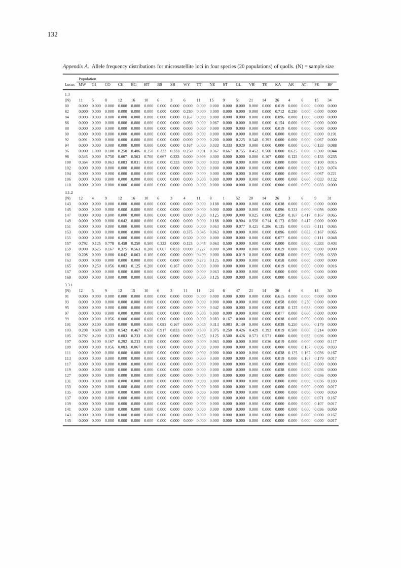
Appendix A.Allele frequency distributions for microsatellite loci in four species (20 populations) of quolls. (N) = sample size

PopulationLocus MW GI CO CH BG BT BS SB WY TT NE ST GL VB TE KA AR AT PE BF

1.3

(N) 11 5 8 12 16 10 6 3 6 11 15 9 51 21 14 26 4 6 15 34

80 0.000 0.000 0.000 0.000 0.000 0.000 0.000 0.000 0.000 0.000 0.000 0.000 0.000 0.000 0.000 0.019 0.000 0.000 0.000 0.00082 0.000 0.000 0.000 0.000 0.000 0.000 0.000 0.000 0.250 0.000 0.000 0.000 0.000 0.000 0.000 0.712 0.250 0.000 0.000 0.000

84 0.000 0.000 0.000 0.000 0.000 0.000 0.000 0.000 0.167 0.000 0.000 0.000 0.000 0.000 0.000 0.096 0.000 1.000 0.000 0.000

86 0.000 0.000 0.000 0.000 0.000 0.000 0.000 0.000 0.083 0.000 0.067 0.000 0.000 0.000 0.000 0.154 0.000 0.000 0.000 0.000

88 0.000 0.000 0.000 0.000 0.000 0.000 0.000 0.000 0.000 0.000 0.000 0.000 0.000 0.000 0.000 0.019 0.000 0.000 0.000 0.00090 0.000 0.000 0.000 0.000 0.000 0.000 0.000 0.000 0.083 0.000 0.000 0.000 0.000 0.000 0.000 0.000 0.000 0.000 0.000 0.191

92 0.091 0.000 0.000 0.000 0.000 0.000 0.000 0.000 0.000 0.000 0.200 0.000 0.225 0.548 0.393 0.000 0.000 0.000 0.067 0.000

94 0.000 0.000 0.000 0.000 0.000 0.000 0.000 0.000 0.167 0.000 0.033 0.333 0.020 0.000 0.000 0.000 0.000 0.000 0.133 0.088

96 0.000 1.000 0.188 0.250 0.406 0.250 0.333 0.333 0.250 0.091 0.367 0.667 0.755 0.452 0.500 0.000 0.625 0.000 0.300 0.04498 0.545 0.000 0.750 0.667 0.563 0.700 0.667 0.333 0.000 0.909 0.300 0.000 0.000 0.000 0.107 0.000 0.125 0.000 0.133 0.235

100 0.364 0.000 0.063 0.083 0.031 0.050 0.000 0.333 0.000 0.000 0.033 0.000 0.000 0.000 0.000 0.000 0.000 0.000 0.100 0.015

102 0.000 0.000 0.000 0.000 0.000 0.000 0.000 0.000 0.000 0.000 0.000 0.000 0.000 0.000 0.000 0.000 0.000 0.000 0.133 0.074104 0.000 0.000 0.000 0.000 0.000 0.000 0.000 0.000 0.000 0.000 0.000 0.000 0.000 0.000 0.000 0.000 0.000 0.000 0.067 0.221

106 0.000 0.000 0.000 0.000 0.000 0.000 0.000 0.000 0.000 0.000 0.000 0.000 0.000 0.000 0.000 0.000 0.000 0.000 0.033 0.132

110 0.000 0.000 0.000 0.000 0.000 0.000 0.000 0.000 0.000 0.000 0.000 0.000 0.000 0.000 0.000 0.000 0.000 0.000 0.033 0.000

3.1.2(N) 12 4 9 12 16 10 6 3 4 11 8 1 52 20 14 26 3 6 9 31

143 0.000 0.000 0.000 0.000 0.000 0.000 0.000 0.000 0.000 0.000 0.188 0.000 0.000 0.000 0.000 0.038 0.000 0.000 0.000 0.000

145 0.000 0.000 0.000 0.000 0.000 0.000 0.000 0.000 0.000 0.000 0.000 0.000 0.000 0.000 0.000 0.096 0.333 0.000 0.056 0.000

147 0.000 0.000 0.000 0.000 0.000 0.000 0.000 0.000 0.000 0.000 0.125 0.000 0.000 0.025 0.000 0.250 0.167 0.417 0.167 0.065149 0.000 0.000 0.000 0.042 0.000 0.000 0.000 0.000 0.000 0.000 0.188 0.000 0.904 0.550 0.714 0.173 0.500 0.417 0.000 0.000

151 0.000 0.000 0.000 0.000 0.000 0.000 0.000 0.000 0.000 0.000 0.063 0.000 0.077 0.425 0.286 0.135 0.000 0.083 0.111 0.065

153 0.000 0.000 0.000 0.000 0.000 0.000 0.000 0.000 0.375 0.045 0.063 0.000 0.000 0.000 0.000 0.096 0.000 0.083 0.167 0.065

155 0.000 0.000 0.000 0.000 0.000 0.000 0.000 0.000 0.500 0.000 0.000 0.000 0.000 0.000 0.000 0.077 0.000 0.000 0.111 0.048157 0.792 0.125 0.778 0.458 0.250 0.500 0.333 0.000 0.125 0.045 0.063 0.500 0.000 0.000 0.000 0.000 0.000 0.000 0.333 0.403

159 0.000 0.625 0.167 0.375 0.563 0.200 0.667 0.833 0.000 0.227 0.000 0.500 0.000 0.000 0.000 0.019 0.000 0.000 0.000 0.000

161 0.208 0.000 0.000 0.042 0.063 0.100 0.000 0.000 0.000 0.409 0.000 0.000 0.019 0.000 0.000 0.038 0.000 0.000 0.056 0.339163 0.000 0.000 0.000 0.000 0.000 0.000 0.000 0.000 0.000 0.273 0.125 0.000 0.000 0.000 0.000 0.058 0.000 0.000 0.000 0.000

165 0.000 0.250 0.056 0.083 0.125 0.200 0.000 0.167 0.000 0.000 0.000 0.000 0.000 0.000 0.000 0.019 0.000 0.000 0.000 0.016

167 0.000 0.000 0.000 0.000 0.000 0.000 0.000 0.000 0.000 0.000 0.063 0.000 0.000 0.000 0.000 0.000 0.000 0.000 0.000 0.000

169 0.000 0.000 0.000 0.000 0.000 0.000 0.000 0.000 0.000 0.000 0.125 0.000 0.000 0.000 0.000 0.000 0.000 0.000 0.000 0.000

3.3.1

(N) 12 5 9 12 15 10 6 3 11 11 24 6 47 21 14 26 4 6 14 30

91 0.000 0.000 0.000 0.000 0.000 0.000 0.000 0.000 0.000 0.000 0.000 0.000 0.000 0.000 0.000 0.615 0.000 0.000 0.000 0.000

93 0.000 0.000 0.000 0.000 0.000 0.000 0.000 0.000 0.000 0.000 0.000 0.000 0.000 0.000 0.000 0.058 0.000 0.250 0.000 0.00095 0.000 0.000 0.000 0.000 0.000 0.000 0.000 0.000 0.000 0.000 0.042 0.000 0.000 0.000 0.000 0.038 0.125 0.083 0.000 0.000

97 0.000 0.000 0.000 0.000 0.000 0.000 0.000 0.000 0.000 0.000 0.000 0.000 0.000 0.000 0.000 0.077 0.000 0.000 0.000 0.000

99 0.000 0.000 0.056 0.000 0.000 0.000 0.000 0.000 1.000 0.000 0.083 0.167 0.000 0.000 0.000 0.038 0.000 0.000 0.000 0.000101 0.000 0.100 0.000 0.000 0.000 0.000 0.083 0.167 0.000 0.045 0.313 0.083 0.149 0.000 0.000 0.038 0.250 0.000 0.179 0.000

103 0.208 0.600 0.389 0.542 0.467 0.650 0.917 0.833 0.000 0.500 0.375 0.250 0.426 0.429 0.393 0.019 0.500 0.000 0.214 0.000

105 0.792 0.200 0.333 0.083 0.233 0.200 0.000 0.000 0.000 0.455 0.125 0.500 0.426 0.571 0.571 0.000 0.000 0.083 0.036 0.000

107 0.000 0.100 0.167 0.292 0.233 0.150 0.000 0.000 0.000 0.000 0.063 0.000 0.000 0.000 0.036 0.019 0.000 0.000 0.000 0.117109 0.000 0.000 0.056 0.083 0.067 0.000 0.000 0.000 0.000 0.000 0.000 0.000 0.000 0.000 0.000 0.000 0.000 0.167 0.036 0.033

111 0.000 0.000 0.000 0.000 0.000 0.000 0.000 0.000 0.000 0.000 0.000 0.000 0.000 0.000 0.000 0.038 0.125 0.167 0.036 0.167

113 0.000 0.000 0.000 0.000 0.000 0.000 0.000 0.000 0.000 0.000 0.000 0.000 0.000 0.000 0.000 0.019 0.000 0.167 0.179 0.017

117 0.000 0.000 0.000 0.000 0.000 0.000 0.000 0.000 0.000 0.000 0.000 0.000 0.000 0.000 0.000 0.000 0.000 0.083 0.000 0.000119 0.000 0.000 0.000 0.000 0.000 0.000 0.000 0.000 0.000 0.000 0.000 0.000 0.000 0.000 0.000 0.038 0.000 0.000 0.036 0.000

127 0.000 0.000 0.000 0.000 0.000 0.000 0.000 0.000 0.000 0.000 0.000 0.000 0.000 0.000 0.000 0.000 0.000 0.000 0.036 0.000

131 0.000 0.000 0.000 0.000 0.000 0.000 0.000 0.000 0.000 0.000 0.000 0.000 0.000 0.000 0.000 0.000 0.000 0.000 0.036 0.183

133 0.000 0.000 0.000 0.000 0.000 0.000 0.000 0.000 0.000 0.000 0.000 0.000 0.000 0.000 0.000 0.000 0.000 0.000 0.000 0.017135 0.000 0.000 0.000 0.000 0.000 0.000 0.000 0.000 0.000 0.000 0.000 0.000 0.000 0.000 0.000 0.000 0.000 0.000 0.000 0.050

137 0.000 0.000 0.000 0.000 0.000 0.000 0.000 0.000 0.000 0.000 0.000 0.000 0.000 0.000 0.000 0.000 0.000 0.000 0.071 0.167

139 0.000 0.000 0.000 0.000 0.000 0.000 0.000 0.000 0.000 0.000 0.000 0.000 0.000 0.000 0.000 0.000 0.000 0.000 0.107 0.017

141 0.000 0.000 0.000 0.000 0.000 0.000 0.000 0.000 0.000 0.000 0.000 0.000 0.000 0.000 0.000 0.000 0.000 0.000 0.036 0.050143 0.000 0.000 0.000 0.000 0.000 0.000 0.000 0.000 0.000 0.000 0.000 0.000 0.000 0.000 0.000 0.000 0.000 0.000 0.000 0.167

145 0.000 0.000 0.000 0.000 0.000 0.000 0.000 0.000 0.000 0.000 0.000 0.000 0.000 0.000 0.000 0.000 0.000 0.000 0.000 0.017

133

Appendix A.Continued

Population

Locus MW GI CO CH BG BT BS SB WY TT NE ST GL VB TE KA AR AT PE BF

3.3.2(N) 11 4 8 12 16 5 5 3 6 10 23 3 51 21 14 24 2 6 9 35

108 0.000 0.000 0.000 0.000 0.000 0.000 0.000 0.000 0.000 0.050 0.000 0.000 0.000 0.000 0.000 0.000 0.000 0.000 0.000 0.000

110 0.000 0.000 0.000 0.000 0.000 0.000 0.000 0.000 0.000 0.000 0.022 0.000 0.000 0.000 0.000 0.000 0.000 0.000 0.056 0.271114 0.545 0.000 0.125 0.000 0.156 0.000 0.200 0.000 0.000 0.050 0.065 0.000 0.000 0.000 0.000 0.000 0.000 0.000 0.000 0.000

116 0.000 0.500 0.500 0.542 0.438 0.800 0.600 0.500 0.000 0.200 0.087 0.000 0.000 0.000 0.000 0.042 0.000 0.167 0.000 0.000

118 0.000 0.500 0.063 0.000 0.000 0.000 0.100 0.333 0.000 0.250 0.261 0.333 0.000 0.000 0.000 0.063 0.000 0.000 0.000 0.014

120 0.455 0.000 0.313 0.292 0.313 0.200 0.100 0.000 0.000 0.400 0.565 0.000 0.000 0.000 0.000 0.000 0.000 0.000 0.111 0.043124 0.000 0.000 0.000 0.000 0.031 0.000 0.000 0.167 0.000 0.000 0.000 0.000 0.000 0.000 0.000 0.063 0.000 0.000 0.000 0.000

126 0.000 0.000 0.000 0.000 0.000 0.000 0.000 0.000 0.167 0.000 0.000 0.000 0.000 0.143 0.000 0.125 0.000 0.083 0.000 0.014

128 0.000 0.000 0.000 0.042 0.063 0.000 0.000 0.000 0.000 0.050 0.000 0.000 0.000 0.024 0.000 0.292 0.000 0.000 0.000 0.000

130 0.000 0.000 0.000 0.000 0.000 0.000 0.000 0.000 0.083 0.000 0.000 0.000 0.225 0.024 0.000 0.000 0.750 0.083 0.056 0.014132 0.000 0.000 0.000 0.000 0.000 0.000 0.000 0.000 0.667 0.000 0.000 0.333 0.000 0.000 0.000 0.042 0.000 0.500 0.000 0.271

134 0.000 0.000 0.000 0.125 0.000 0.000 0.000 0.000 0.083 0.000 0.000 0.000 0.235 0.167 0.214 0.021 0.250 0.000 0.167 0.086

136 0.000 0.000 0.000 0.000 0.000 0.000 0.000 0.000 0.000 0.000 0.000 0.000 0.049 0.000 0.000 0.083 0.000 0.000 0.167 0.000

138 0.000 0.000 0.000 0.000 0.000 0.000 0.000 0.000 0.000 0.000 0.000 0.000 0.147 0.310 0.321 0.104 0.000 0.083 0.167 0.200140 0.000 0.000 0.000 0.000 0.000 0.000 0.000 0.000 0.000 0.000 0.000 0.000 0.137 0.262 0.321 0.021 0.000 0.000 0.000 0.000

142 0.000 0.000 0.000 0.000 0.000 0.000 0.000 0.000 0.000 0.000 0.000 0.000 0.196 0.071 0.071 0.063 0.000 0.083 0.111 0.000

144 0.000 0.000 0.000 0.000 0.000 0.000 0.000 0.000 0.000 0.000 0.000 0.000 0.010 0.000 0.071 0.021 0.000 0.000 0.056 0.071

146 0.000 0.000 0.000 0.000 0.000 0.000 0.000 0.000 0.000 0.000 0.000 0.333 0.000 0.000 0.000 0.021 0.000 0.000 0.056 0.000148 0.000 0.000 0.000 0.000 0.000 0.000 0.000 0.000 0.000 0.000 0.000 0.000 0.000 0.000 0.000 0.042 0.000 0.000 0.056 0.014

4.4.2

(N) 12 5 9 12 16 11 6 3 26 11 18 0 55 21 13 26 9 6 9 3470 0.000 0.000 0.000 0.000 0.000 0.000 0.000 0.000 0.000 0.000 0.083 – 0.000 0.000 0.000 0.154 0.000 0.000 0.000 0.000

74 0.000 0.000 0.000 0.000 0.000 0.000 0.000 0.000 0.019 0.000 0.000 – 0.000 0.000 0.000 0.000 0.000 0.000 0.000 0.000

76 0.000 0.000 0.000 0.000 0.000 0.045 0.000 0.333 0.058 0.000 0.028 – 0.000 0.000 0.000 0.000 0.000 0.000 0.000 0.000

78 0.000 0.000 0.000 0.000 0.000 0.045 0.000 0.000 0.019 0.000 0.056 – 0.000 0.000 0.000 0.000 0.000 0.000 0.056 0.14780 0.458 0.200 0.222 0.208 0.219 0.045 0.000 0.000 0.019 0.000 0.056 – 0.000 0.000 0.000 0.000 0.167 0.000 0.000 0.029

82 0.000 0.700 0.222 0.375 0.156 0.182 0.000 0.000 0.250 0.091 0.083 – 0.000 0.000 0.000 0.000 0.167 0.083 0.167 0.250

84 0.000 0.000 0.167 0.083 0.094 0.136 0.250 0.000 0.385 0.545 0.222 – 0.000 0.000 0.000 0.038 0.500 0.000 0.278 0.147

86 0.000 0.000 0.167 0.250 0.125 0.318 0.167 0.500 0.115 0.364 0.000 – 0.000 0.000 0.000 0.019 0.000 0.167 0.056 0.00088 0.000 0.000 0.056 0.000 0.063 0.091 0.583 0.167 0.000 0.000 0.083 – 0.000 0.000 0.000 0.154 0.000 0.500 0.111 0.029

90 0.292 0.100 0.167 0.083 0.344 0.136 0.000 0.000 0.000 0.000 0.056 – 0.109 0.000 0.000 0.231 0.056 0.000 0.167 0.338

92 0.250 0.000 0.000 0.000 0.000 0.000 0.000 0.000 0.000 0.000 0.056 – 0.018 0.071 0.038 0.250 0.000 0.083 0.111 0.000

94 0.000 0.000 0.000 0.000 0.000 0.000 0.000 0.000 0.000 0.000 0.028 – 0.209 0.333 0.000 0.038 0.056 0.167 0.000 0.00096 0.000 0.000 0.000 0.000 0.000 0.000 0.000 0.000 0.135 0.000 0.111 – 0.609 0.167 0.769 0.038 0.056 0.000 0.000 0.000

98 0.000 0.000 0.000 0.000 0.000 0.000 0.000 0.000 0.000 0.000 0.083 – 0.018 0.429 0.192 0.019 0.000 0.000 0.056 0.000

100 0.000 0.000 0.000 0.000 0.000 0.000 0.000 0.000 0.000 0.000 0.056 – 0.000 0.000 0.000 0.058 0.000 0.000 0.000 0.000

102 0.000 0.000 0.000 0.000 0.000 0.000 0.000 0.000 0.000 0.000 0.000 – 0.036 0.000 0.000 0.000 0.000 0.000 0.000 0.015110 0.000 0.000 0.000 0.000 0.000 0.000 0.000 0.000 0.000 0.000 0.000 – 0.000 0.000 0.000 0.000 0.000 0.000 0.000 0.044

4.4.10

(N) 12 4 9 12 15 10 6 3 2 11 2 0 54 21 14 25 0 6 9 33179 0.000 0.000 0.000 0.000 0.000 0.000 0.000 0.000 0.000 0.000 0.000 – 0.000 0.000 0.000 0.720 – 1.000 0.000 0.000

181 0.000 0.000 0.000 0.000 0.000 0.000 0.000 0.000 0.000 0.000 0.000 – 0.000 0.000 0.000 0.260 – 0.000 0.000 0.000

183 0.000 0.000 0.000 0.000 0.000 0.000 0.000 0.000 0.000 0.000 0.000 – 0.000 0.000 0.000 0.020 – 0.000 0.000 0.000

187 0.000 0.000 0.111 0.167 0.033 0.150 0.750 0.333 0.500 0.000 0.000 – 0.000 0.000 0.000 0.000 – 0.000 0.056 0.000189 0.000 0.000 0.000 0.000 0.100 0.000 0.000 0.000 0.000 0.000 0.000 – 0.009 0.000 0.036 0.000 – 0.000 0.000 0.000

191 0.000 0.000 0.000 0.042 0.000 0.000 0.000 0.000 0.000 0.000 0.250 – 0.009 0.524 0.143 0.000 – 0.000 0.000 0.000

193 0.667 0.000 0.167 0.417 0.333 0.050 0.250 0.000 0.250 0.000 0.000 – 0.009 0.000 0.071 0.000 – 0.000 0.000 0.000

195 0.042 0.000 0.278 0.083 0.033 0.150 0.000 0.000 0.000 0.500 0.500 – 0.000 0.000 0.000 0.000 – 0.000 0.000 0.000197 0.000 0.125 0.278 0.083 0.467 0.300 0.000 0.667 0.250 0.227 0.000 – 0.000 0.000 0.000 0.000 – 0.000 0.000 0.000

199 0.292 0.375 0.167 0.167 0.033 0.350 0.000 0.000 0.000 0.227 0.250 – 0.000 0.000 0.000 0.000 – 0.000 0.000 0.015

201 0.000 0.500 0.000 0.042 0.000 0.000 0.000 0.000 0.000 0.000 0.000 – 0.000 0.000 0.000 0.000 – 0.000 0.167 0.030203 0.000 0.000 0.000 0.000 0.000 0.000 0.000 0.000 0.000 0.045 0.000 – 0.000 0.000 0.000 0.000 – 0.000 0.000 0.091

205 0.000 0.000 0.000 0.000 0.000 0.000 0.000 0.000 0.000 0.000 0.000 – 0.000 0.000 0.000 0.000 – 0.000 0.278 0.288

207 0.000 0.000 0.000 0.000 0.000 0.000 0.000 0.000 0.000 0.000 0.000 – 0.000 0.000 0.000 0.000 – 0.000 0.167 0.152

209 0.000 0.000 0.000 0.000 0.000 0.000 0.000 0.000 0.000 0.000 0.000 – 0.009 0.000 0.000 0.000 – 0.000 0.111 0.212211 0.000 0.000 0.000 0.000 0.000 0.000 0.000 0.000 0.000 0.000 0.000 – 0.269 0.000 0.000 0.000 – 0.000 0.111 0.152

213 0.000 0.000 0.000 0.000 0.000 0.000 0.000 0.000 0.000 0.000 0.000 – 0.667 0.024 0.286 0.000 – 0.000 0.111 0.030

215 0.000 0.000 0.000 0.000 0.000 0.000 0.000 0.000 0.000 0.000 0.000 – 0.028 0.452 0.393 0.000 – 0.000 0.000 0.015

217 0.000 0.000 0.000 0.000 0.000 0.000 0.000 0.000 0.000 0.000 0.000 – 0.000 0.000 0.071 0.000 – 0.000 0.000 0.015