JOURNAL OF RESEARCH of the National Bureau of Standards —A. Physics and ChemistryVol. 81 A, No. 1, January-February 1977

Vapor Pressure Formulation for Ice

Arnold Wexler

Institute for Basic Standards, National Bureau of Standards, Washignton, D.C. 20234

(September 23, 1976)

A new formulation is presented for the vapor pressure of ice from the triple point to —100 °C based onthermodynamic calculations. Use is made of the definitive experimental value of the vapor pressure of water at itstriple point recently obtained by Guildner, Johnson, and Jones. A table is given of the vapor pressure as a functionof temperature at 0.1-degree intervals over the range 0 to —100 °C, together with the values of the temperaturederivative at 1-degree intervals. The formulation is compared with published experimental measurements andvapor pressure equations. It is estimated that this formulation predicts the vapor pressure of ice with an overalluncertainty that varies from 0.016 percent at the triple point to 0.50 percent at —100 °C.

Key words: Clausius-Clapeyron equation; saturation vapor pressure over ice; thermal properties of ice; vaporpressure; vapor pressure at the triple point; vapor pressure of ice; water vapor.

1. Introduction

In meteorology, air conditioning, and hygrometry, particu-larly in the maintenance and use of standards and generatorsin calibrations and in precision measurements, accurate val-ues of the vapor pressure of the pure water-substance areessential. Because of this Wexler and Greenspan [I]1 re-cently published a new vapor pressure formulation for thepure liquid phase, based on thermodynamic calculations,which is in excellent agreement from 25 to 100 °C with theprecise measurements of Stimson [2]. Wexler [3] subse-quently revised this formulation to make it consistent with thedefinitive experimental value of the vapor pressure of water atits triple point obtained by Guildner, Johnson, and Jones.The purpose of this present paper is to apply a similar methodof calculation to the pure ice phase and derive a new formula-tion for temperatures down to —100 °C. This new formulationfor ice is constrained to yield the identical value of vaporpressure at the triple point as that given by the revisedformulation for the liquid phase.

A critical examination of the experimental vapor-pressuredata of ice discloses the disconcerting fact that the dispersionamong those values far exceeds modern accuracy require-ments. This dispersion arises, in part, from the inherentdifficulties experienced by investigators in making precisionmeasurements of these low pressures and from the ambigui-ties in the temperature scale used in the early 1900's whenseveral major series of determinations were made. Thermody-namic calculations, based on accurate thermal data, providean alternate route to the determination of vapor pressure. It istherefore not surprising that such calculations have beenmade repeatedly for ice with varying degrees of success. It isinteresting to note that these calculations have been preferredover the existent experimental vapor pressures, primarilybecause the calculations appear to yield less uncertainty thanthe measurements.

1 Figures in brackets indicate the literature references at the end of this paper.

2. Derivation

The Clausius-Clapeyron equation, when applied to thesolid-vapor phase transition for the pure water-substance,may be written

dp _ I

dT " T(v - v")(1)

where p is the pressure of the saturated vapor, v is thespecific volume of the saturated vapor, v" is the specificvolume of the saturated ice, T is the absolute thermodynamictemperature, / is the latent heat of sublimation, and dp/dT isthe derivative of the vapor pressure with respect to tempera-ture. The latent heat of sublimation is given by

1 = h- h" (2)

where h is the specific enthalpy of saturated water vapor attemperature T and h" is the specific enthalpy of saturated iceat the same temperature T.

The equation of state for saturated water vapor may beexpressed by

pv = ZRT (3)

where Z is the compressibility factor and R is the specific gasconstant. When eq (3) is substituted into eq (1) the result is

dp

P

I

ZRT2 1 + -)v )

dT (4)

where higher order terms of v"/v are neglected because v"/v« 1. On integrating, eq (4) becomes

T2

where px and/>2 are the saturation vapor pressures at temper-atures 7\ and T2, respectively. Suitable functions will besought forZ, v9 v" and / in order to complete the integration ofeq (5).

Functions for the compressibility factor Z and the specificvolume of saturated water vapor v will be based on a virialequation of state expressed as a power series in p. A functionfor the specific volume of saturated ice v" will be developedfrom experimental data for the coefficient of linear expansionand the density at 0 °C. A function for the latent heat ofsublimation / will be derived from the specific enthalpies h"and h of saturated ice and saturated water vapor, respec-tively. Use will be made of measurements of the specific heatof ice to obtain h" whereas statistical mechanical calculationsof the ideal-gas (zero-pressure) specific heat of water willserve as input data for establishing an expression for h.

2.1 Temperature

Guildner and Edsinger [5] have recently made measure-ments on the realization of the thermodynamic temperaturescale from 273.16 to 730 K by means of gas thermometry.Unfortunately there are no similar high precision measure-ments below 273.16 K. Therefore, it will be assumed that theInternational Practical Temperature Scale of 1968 (IPTS-68)[6] is a sufficiently close approximation to the absolutethermodynamic temperature so that the thermal quantitiesgiven in terms of IFTS-68 can be used in eq (5). From thetriple point to —100 °C the temperature t in degrees Celsiushas the same numerical values on the International Tempera-ture Scale of 1927 (ITS-27) [7], the International Tempera-ture Scale of 1948 (ITS-48) [8] and the International PracticalTemperature Scale of 1948 (IPTS-48) [9]. However, the icepoint on IPTS-48 is defined as equal to 273.15 kelvinswhereas on ITS-27 and ITS-48 it is defined as equal to273.16 kelvins. The difference T6S — T4S, where T6S and T48are the kelvin temperatures on IPTS-68 and IPTS-48, respec-tively, in the range of interest reaches a maximum of 0.0336kelvin at 200 K [10, 11]. Using the corrections given byRiddle, Furukawa, and Plumb [11], temperatures on ITS-27,ITS-48 and IPTS-48 have been converted to IPTS-68 whereneeded in the calculations.

2.2. Specific Volume of Saturated Vapor

Equation (3) is used to calculate the specific volume ofsaturated water vapor v. The compressibility factor Z isexpressed as a power series in p

z = + cy + (6)

where B' is the second pressure-series virial coefficient andC is the third pressure-series virial coefficient. The contri-bution oiC'p2 toZ is only a few parts per million at the triplepoint and less at lower temperatures and so has negligibleeffect. The empirical relationship for the second virial coeffi-cient is based on experimental data obtained at elevatedtemperatures. This equation will be extrapolated below 0 °Cwith the full recognition that this may lead to large uncertain-ties in the virial coefficients. Although Z?' rapidly increasesin magnitude with decreasing temperature, the saturationvapor pressure decreases even more rapidly so that Z rapidly

approaches its limiting value of unity as the temperaturedrops. Saturated water vapor, therefore, tends to behave moreand more like an ideal gas as the temperature decreases,thereby reducing the effect of errors in B'.

Table 1 shows a comparison of Z from the triple point to— 100 °C, for water vapor saturated with respect to ice,calculated using the empirical second virial coefficient equa-tions of Goff and Gratch [12, 13, 14], Keyes [15, 16], andJuza as given by Bain [17]. The maximum difference inZ, aswell as v, is 118 ppm and occurs at 0.01 °C. This can be usedas an indication of uncertainty although the actual error isindeterminate. The differences decrease as the temperaturedecreases. At —70 °C and below, the differences are equalto, or less than, one ppm since, at such temperatures, thesecond virial coefficient makes a negligible contribution toZ.

TABLE 1. Compressibility factor for saturated water vaporover ice

Temperature

°c

0.010

-10-20-30-40-50-60-70-80-90

-100

Keyes1969 b

Z0.999624.999624.999907.999958.999982.999993.999998.9999991.0000001.0000001.0000001.000000

Compressibility Factor0

Keves1947 c

Z0.999501.999501.999726.999856.999928.999966.999984.999994.999997.9999991.0000001.000000

Baind

Z0.999529.999529.999747.999871.999938.999972.999986.999996.999999

1.0000001.0000001.000000

Goffand

Gratch e

Z0.999506.999506.999730.999859.999930.999967.999985.999994.999998.9999991.0000001.000000

a Calculated by eq (6) using B ' given by the indicated investigator.6 Ref [16].c Ref [15].d Ref [17].e Ref [12-14].

The 1969 second virial coefficient of Keyes [16] will beused in order to be consistent with the earlier use of this samecoefficient [3]. His virial coefficient equation, converted to SIunits compatible with eq (6), is

_ [0.44687 /565.965X

x 10 34900 + r- x 1O~5. (7)

where B' is in units of reciprocal pressure (Pa)"1.2

2.3. Specific Volume of Saturated Ice

Only hexagonal Ice-I will be of concern. It will be assumedthat the crystals are randomly aligned with respect to theoptic axis. All known measurements of the density of ice havebeen made in the presence of an inert gas, usually at apressure of one atmosphere and at a temperature of 0 °C.

: 1 Pa = 1 N/m2 = 10"5 bar = 10"2 mb = 7.50062 X 10"3 mm Hg.

Dorsey [18] has compiled an extensive list of such determina-tions. Ginnings and Corruccini [19] using a Bunsen icecalorimeter, obtained a value at 0 °C and one atmosphere3 of0.91671 g/ml. This value is definitive and supersedes allearlier measurements. Using this value and the coefficient oflinear expansion of ice, the specific volume was calculated attemperatures below 0 °C as follows.

The isopiestic coefficient of linear expansion of ice otp isdefined by the equation

) (8)

where A.j is the initial length of a specimen at the ice pointtemperature, A is the length of the same specimen at temper-ature T and dk/dT is the rate of thermal expansion. Byintegrating eq (8), cubing the resultant equation, neglecting

(9)

higher order terms in I otpdT', it follows that

p T — V P i T + 3 f etp dA

where f "p,r is the specific volume of ice at pressure P andtemperature T, v"P}T. is the specific volume of ice at pressureP and at the ice point temperature T\.

There are several series of measurements of the coefficientof linear expansion of hexagonal Ice-I at atmospheric pres-sure. The data of Jakob and Erk [20], Powell [21], Butkovich[22], Dantl [23], and LaPlaca and Post [24] were fitted to alinear equation by the method of least squares. The result is

temperature, v" is the specific volume, f3 is the volumeexpansivity, and c"p is the specific heat at constant pressure.Values of the isothermal compressibility of ice were calcu-lated by using Leadbetter's values [27] for the adiabaticcompressibility of Ice-I, eq (11) to obtain the specific volumeat pressure Pa and temperature 7\ eq (10) to obtain ft ( =3apa), and eq (19) (which is derived later) to obtain thespecific heat at constant pressure Pa. The results for thetemperature range of interest are given by the linear equation

k = (8.875 + 0.016571) X 10~u (13)

where k is expressed in units of (Pa) *. The specific volumeof ice at pressure P and temperature T is therefore v"p T —t/'po,7[l " k(P ~ Pa)] SO that

V"P.T = vnPatT[\ - (8.875 + 0.0165r)(P - 101325)

X 10"11] (14)

where P is expressed in Pa. If the saturated vapor pressure pis inserted forP, then eq (14) yields the pure phase specificvolume v" at saturation. Over the temperature range 173.15to 273.16 K the numerical value of the bracket is equal to1.000013 with a maximum variability of one ppm. Using thisvalue yields

V"P,T = v" = 1.070003 - 0.249936 X 10"4 T

+ 0.371611 X 10"6r2 . (15)

X 106 = -7.6370 + 0.227097 T (10)2.4 Enthalpy of Ice

which, when substituted into eq (9) together with the Gin-nings and Corruccini value4 for the density of ice at 0 °C and It can be shown [26] that the specific enthalpy h" of theone atmosphere becomes s°lid phase of a pure substance, say ice, is given by the

relationship

v"Pa,T = 1.069989 - 0.249933 X 10"4 T

+ 0.371606 X 10" 6 r 2 (11)

where v"pa>T, expressed in cm3/g, is the specific volume atatmospheric pressure, i.e., 101325 Pa, and temperature T. Itis the specific volume at saturation rather than at atmosphericpressure that is needed. The specific volume at a givenpressure can be corrected to that at another pressure from aknowledge of the isothermal compressibility A:, which is givenby the equation

k = Lit

c p(12)

where ks is the adiabatic compressibility, T is the absolute

3 1 atmosphere = 101325 pascals.4 The density was converted from g/ml to g/cm3 by using the factor 1 ml = 1.000028 cm3 [25].

dh" = c"P dT + v"T dP -dT

dP (16)

where c"P is the specific heat of ice at constant pressure P.When integrated this equation becomes

Because eq (17) represents a system undergoing a reversi-ble process between two equilibrium states, the initial andfinal enthalpies are independent of the path. Therefore, apath is chosen which starts on the saturation curve at (7^, p^),moves isothermally to (7^, Pa), then proceeds isobarically to(7\ Pa), and finally goes isothermally to (7\ p). The integra-tion along this path is given by

If pi is the saturation vapor pressure at the ice-point tempera-ture Tf, p is the saturation vapor pressure at temperature 7\and Pa is any other pressure, say standard atmosphericpressure, then h" — h!\ is the difference in specific enthalpyof saturated ice, under its own equilibrium vapor pressure,between temperatures T and 7Y

Although measurements of the isopiestic specific heat ofice have been made by several investigators [28-35], onlythose of Giauque and Stout [34] will be used because it isbelieved that these are the best available over the range oftemperatures of interest here. These measurements weremade at standard atmospheric pressure and cover the temper-ature range 16.43 to 267.77 K. They are in good agreementwith the precise measurements of Dickinson and Osborne[30]. Unfortunately, the latter measurements do not extendbelow 233.15 K.

Fitting the Giauque and Stout data from 169.42 to 267.77K to a quadratic equation by the method of least squares withthe temperature converted to IPTS-68 and the heat units tojoules, yields

c"P = Ao + AJ + A2T2 (19)

where c"pa is the specific heat in J/gK at a pressure of oneatmosphere. The coefficients are given in table 2. Integratingeq (19), one obtains

r dT = A0{T - Tt)

(20)

By letting

=JPPi W/J

and performing the indicated differentiations and integra-tions, eq (21) is reduced to the form

A/i" = Bo + BJ2 + B2p (22)

+ — (T3 - T?) + A/i". (23)

A numerical value remains to be assigned to the referenceenthalpy h"i. At any specified temperature T, the latent heatof fusion of ice /" is given by

/" = h' - K' (24)

where h' and h" are the specific enthalpies of liquid waterand ice, respectively. By adopting the convention h'i = 0 atthe ice-point temperature it follows that l"i = —h"i. Thechoice of this convention will not effect the final resultsbecause the arbitrary assignment will cancel out in thecomputations. Use is now made of the experimentally deter-mined value for the latent heat of fusion of ice at 0 °C andstandard atmospheric pressure recommended by Osborne[36]5, namely, 333.535 J/g. By means of the thermodynamicrelationship

dh dv(25)

the latent heat was adjusted from standard atmospheric pres-sure (101325 Pa) to the saturation vapor pressure of ice at 0°C, i.e., 611 Pa, yielding V\ = -h"t = 333.430 J/g. Equa-tion (23) therefore becomes

h" = -l"t + A0(T - Tt) + ^ (T2 - T?)

+ — (T3 - Tt3) + A/i" (26)

2.5. Enthalphy of Water Vapor

From eqs (3) and (6) it follows that

RTv = — (l+B'p + C'p2

P(27)

and

RT

P

dB'£ + • • • ) m

which on substitution into eq (25) yield

dC

dp

razr + d_c_+ _ iLdT dT J

wherep is the saturation vapor pressure in Pa at temperature Integration with respect top leads tor , Pa = 101325 Pa and/?* = 611 Pa. The coefficients are f f

given in table 2. Substitution of eqs (20) and (22) into (18) , __ , _ 0^2 ^ L _ 1/ 7 2 _ - p 2 _yields P'T P°'T dT 2 dT

(29)

(30)

h" = H\ + A0(T -Td + — (T2 - Tt2) 5 The value given by Osborne was converted from international joules to absolute joules by the

factor 1.000165 J = 1 i.j.

8

where JIP)T is the enthalpy of water vapor at saturation pres-sure p and temperature T and hPo>T is the ideal-gas (zero-pressure) specific enthalpy at the same temperature T. Thethird and higher-order terms will be ignored because theircontributions to hp>T are negligible. Thus, by setting

the result can be written

(31)

(32)

Friedman and Haar [37] have calculated the ideal-gas(zero-pressure) specific heat cpjR for water vapor from sta-tistical mechanical considerations over a wide range of tem-peratures. Their calculated values from 170 to 280 K werefitted to a polynomial equation by the method of least squareswhich, after multiplying by R, has the form

= A) + + D2T2 + D3T

S (33)

in units of J/gK. The coefficients are given in table 2.Integrating with respect to temperature from the ice pointtemperature T\ to T, one gets

P0,T ~ hpo,Tt ~ CPQ

JTi

dT (34)

which becomes

= D0(T - -r(T2~m

—(T3- 7V) + — (T4 - 7V)o 4

(35)

I' = h - h'. (36)

It will be recalled that the convention that h\ = 0 at the icepoint has already been adopted. Hence at this temperaturehi = I'i, with the result that eq (32) becomes

where

(37)

(38)

Replacing hi by Vi in eq (37), one obtains

hPQsTi = I'i + A/i*. (39)

Substituting eq (39) into eq (35) gives rise to an expressionfor the ideal-gas specific enthalpy of water vapor, that is,

V.r = l't+Aht + D0(T -Ti) + - (T2 - 7?)

+ V(T3 ~ 7?) + j-{T* - m. (40)

Now by inserting eq (40) into (32) the real-gas specificenthalpy of saturated water vapor ensu^ , namely,

h = hPiT = I'i + Hhi - Ah + D0(T - Ti)

To calculate V i, use is made of an approach due to Osborne[38] which starts with the definition of an experimentallymeasured calorimetric quantity y

V = y - 8. (42)where /*pD,r a nd bpo,Tt are the ideal-gas (zero-pressure) spe-cific enthalpies of water vapor at temperatures T and Tt in y h a s b e e n q u i t e a c c u r a t e l y measured [38-41]. 8 is given byunits of J/g. [38]

The ideal gas specific enthalphy hPo>Tt is a constant towhich a numerical value must be assigned. In order to do souse is made of the latent heat of vaporization V at the ice 8point. By definition ^v v

TABLE 2. Coefficients to equations

ABDFGHKL

0

0.274292-0.344 X lO-2

.1834928 x

.34238440 x-0.57284294 X-0.1369402 X-0.58653696 X-0.57170491 x

101

104

104

103

104

104

1

0.582109 X lO-2

.3765 X 10~7

.2542981 X 10-3

-0.52277204 X 101

.2224103300 X 102

.9158658955 X 101

2

0.325031 X.107 x 10

-0.15852458.98557190

-0.60309325. 19779974.13749042

-0.74950412

10-5

XXXXXX

-5

10-5

10~2

10~2

101

10"1

lO-2

3

0.3550699 X-0.11305118-0.17462428-0.32285532-0.340317750.36067657

X

xX

xX

10 8

lO-4

10-5

lO-4

lO-4

101

4

0.64112408.26326563.26967687

XXX

10-9

10-7

10-7

5

0.33815137 X 101

-0.26896486 X 101

.6918651

where v and v' are the specific volumes of saturated vapor andwater, respectively, and dp/dT is the temperature derivativeof the vapor pressure of liquid water. The quantity y isrepresented with high precision from 273.15 to 423.15 K inunits of J/g by the following polynomial equation [3]

y = Fo + FJ + F2T2 + F3T

3. (44)

The coefficients are given in table 2. At T = 273.15 K, yi =2500.8384 J/g. The quantity 8U at T = 273.15 K, using v' =1.00016 cm3/g [42] and dp/dT = 44.4 Pa/K [3], is 0.0121J/g. Therefore V \ = 2500.8263 J/g. By appropriate substitu-tions into eq (38) one obtains Ahi — 0.2365 J/g.

2.6. Latent Heat of Sublimation

Substitution of eqs (26) and (41) into (2) gives rise to thefollowing equation for the latent heat of sublimation:

- (Do -

-\(DX- AX)T? ~\(D2- A2)T? ~ \

- A0)T + \(DX- A,)

+ -DBT4 - A h - Ah".4

- A2)T*

(45)

2.7 Vapor Pressure

Combining eqs (5) and (45), selecting the temperature 7\and vapor pressure pt at the triple point as the lower limits ofintegration, taking any temperature T and correspondingvapor pressure p as the upper limits, and performing somesimple mathematical manipulations, one obtains

d(\np)

-1 - rr1) + G5 in (Pj=o

~-(D2

G,=

2R

D2 - A2

6R

12R

and G5 =R

(47)

(48)

(49)

(50)

(51)

The coefficients are given in table 2.The first two terms on the right-hand side of eq (46)

provide the major contribution to the vapor pressure; theintegrals are small corrections which account, in part, for thedeviation of water vapor from ideal gas behavior. These havebeen left in integral form because each is a function of/? aswell as T.

The absolute temperature assigned to the triple point onIPTS-68 is 273.16 K. The corresponding vapor pressure is611.657 Pa, the definitive value measured by Guildner,Johnson, and Jones [4]. The specific gas constant for water, R= 0.461520 J/g K, was derived from the CODATA recom-mended value of 8.31441 J/mol K for the universal gasconstant [43], and 18.015227 g for the molar mass of natu-rally occurring water vapor on the unified carbon-12 scale.6

Because eq (46) is implicit in p it had to be solved byiteration. Each of the integrals on the right-hand side wasevaluated at intervals of 0.25 kelvins by means of the trape-zoidal rule [47]. Iteration at each interval was terminatedwhen successive values ofp differed by less than 0.1 ppm.The magnitudes of the terms in eq (46) are shown in skeletonform in table 3. The magnitudes of the integral terms areequivalent to the relative contributions they make to thevapor pressure. The sum of the integrals increases from zeroat the triple point to -0.000389 at -100 °C. Neglecting theintegrals, therefore, would introduce an error of up to 389ppm in the vapor pressure. The sums of the integrals, atintervals of 2 kelvins, were fitted by the method of leastsquares to the equation

integrals = + H5 In (~ (52)

with a residual standard deviation [48] of 0.7 X 10 6. Thecoefficients are given in table 2. Substituting eq (52) into(46), integrating the left-hand side, and combining terms,

vhere Go = — — (yj — 8t + M.t

- (Do - A0)Tt - - ent, respectively. Combining these abundalides, recommended by the Commission on

h l l i h f ll

10

2

!

one finally obtains

In ( - ) = 2 UT*-1 ~ TV1) + ^5 In (J-) (53)\Pt' j=o \Tt/

which reduces to

In p = + ^ 5 In Tj = 0

where ^o = ^o

K5lnTt- In p

A-2 — O2

X4 = G4

K5 = G5

H4

(54)

(55)

(56)

(57)

(58)

(59)

(60)

The coefficients are given in table 2.The feasibility of reducing the number of terms in eqs (53)

and (54) was investigated. Values of vapor pressure weregenerated from eq (53) at one-kelvin intervals from the icepoint to 172.15 K and fitted by the method of least squares toequations of the form

In - 1 = Z, Ljip-1 - Pf1) + Ln+1 In — (61)w i=o vr^/

for 0 < n < 4 with and without the ] term. For n = 2,

71

with the In ( —) term included, the standard deviation of the

fit was 14 pprri and the maximum deviation was 26 ppm.Thus, for n = 2, eq (61) becomes

d (62)\Ptf 3=0

or, alternately,

where

lnp = 2JLjp-1+L3lnT (63)J=0

Li = - ^ ~ L2Tt - L3 In T, + lnp ( (64)

The coefficients are given in table 2.

11

3. Error Analysis

It is of interest to assign reasonable bounds of uncertaintyto the independent variables and constants and then calculatethe effect of these uncertainties on p. Start with eq (5) andrecall that

Z = 1 + B'p

ZRT

(65)

(66)

v" = v"Pa,Ti [ l + 3 f aPa dT~\ \l ~ k(p - P j ] (67)

=1 Cp dT + yi - 8t + Ahi - AhJTi

fT

c"P dT - AH' + t\ (68)

JTi

vhere

and

(69)

Substituting the above equations into eq (5) converts thelatter into a functional relationship of independent variablesand constants. The vapor pressure is calculated by iterationand numerical integration, as previously described. The cal-culation then is repeated with each variable and constantseparately augmented by its appropriate estimated error.

The absolute temperature T enters into eq (5) as theindependent variable so that it is subject neither to experi-mental nor scale error. However, experimental and scaleerrors in the temperature affect the uncertainties in theindependent variables; therefore, these temperature errorsare contained in the estimated errors of the independentvariables. Since Tt is assigned values on IPTS-68, it will beassumed that its estimated uncertainty is zero.

The estimated error in the specific gas constant for watervapor R arises from the assigned (three standard deviations)uncertainty [43] in the molar gas constant of 78 X 10~5 J/molK and from a calculated (three standard deviations) uncer-tainty in the molecular weight of naturally occurring water of9 X 10~5 g/mol based on the assigned uncertainties [46] inthe relative atomic masses of the pertinent nuclides. Theresultant estimated error (three standard deviations) in R is45 X 1(T6 J/g K (94 ppm).

There are no experimental data below 273.15 K on which

to base an estimate of the uncertainty in the virial coefficientB' nor in the derivative dB'/dT. Therefore, four sets ofextrapolated virial coefficients were calculated, using theempirical equations of Goff and Gratch [12-14], Keyes [15,16], and Juza as given by Bain [17], and then differenceswere obtained from the latest Keyes values [16]. The esti-mated uncertainty was set at thrice the maximum difference.This uncertainty in B' contributed to a corresponding uncer-tainty in dB'I dT.

Pa is standard atmospheric pressure. Because this is anassigned value it will be assumed that its uncertainty is zero.

Guildner, Johnson, and Jones [4] have assigned an esti-mated uncertainty (three standard deviations plus systematicerrors) of 0.010 Pa (16 ppm) to their measured value of thevapor pressure at the triple point pt. Their estimated uncer-tainty will be used here.

According to Ginnings and Corruccini [19], the combinedrandom and systematic uncertainty in their determination ofthe density of ice at 0 °C and 1 atmosphere is 0.00005 g/ml.This value was converted to 0.00006 cm3/g and the latterused as the estimated uncertainty in the specific volume ofice v"pa}T.. The estimated uncertainty in the coefficient OLpawill be taken as three times the standard deviation of the fit[48] as given by eq (10), that is, 0.50 X 10~5 cm/cm K.Leadbetter [27] has ascribed an uncertainty of 5 percent tohis values of the adiabatic compressibility of ice, namely 0.6cm3/cm3 Pa. The same uncertainty is therefore used for theisothermal compressibility k, since the latter is derived fromLeadbetter's values.

Friedman and Haar [37] have computed cpjR to sixsignificant figures. However, they did not give an estimate ofthe uncertainty in their calculated values. An error of 100ppm therefore was assigned to cpjR. Combining this erroralong with 99 ppm for the estimated uncertainty in R and 9ppm which represents three times the residual standarddeviation of the fit of eq (33) resulted in an estimated error of140 ppm in CPQ, i.e., 0.26 X 10"3 J/g K.

In the absence of any other criteria for estimating theuncertainty in c'pa, a value of 0.0103 J/g K was selectedwhich equals three times the standard deviation of the fit ofeq (19), 0.0099 J/g K, plus an estimated error of 0.0004 J/gK due to ambiguities in the temperature scale employed byGiauque and Stout.

The estimated error in yt was taken as 0.45 J/g which isthree times the standard deviation of the fit of eq (44). Theuncertainty in 8$ was conservatively estimated at less thanone percent, that is, less than 0.0001 J/g. Osborne [36] hasestimated that the random and systematic error in t[ was 0.2J/g and his value, therefore, was used here.

The quantity Ah" varies from zero at 0 °C to about —0.002J/g at -100 °C. Since it is small compared to / (~ 2830 J/g),its functional dependence on other parameters will be ig-nored. The uncertainty in Ah" was estimated at less than0.0001 J/g.

A summary of the individual estimated errors contributingto the total error in the predicted vapor pressure is given intable 4. The corresponding uncertainty inp due to each of theenumerated errors is shown in table 5. The square root of thesum of the squares of the individual errors was used as thebest estimate of the overall maximum error inp [49]. As thetemperature decreases from the triple point to —100 °C, theestimated relative error in p increases from 16 ppm to 0.5percent.

12

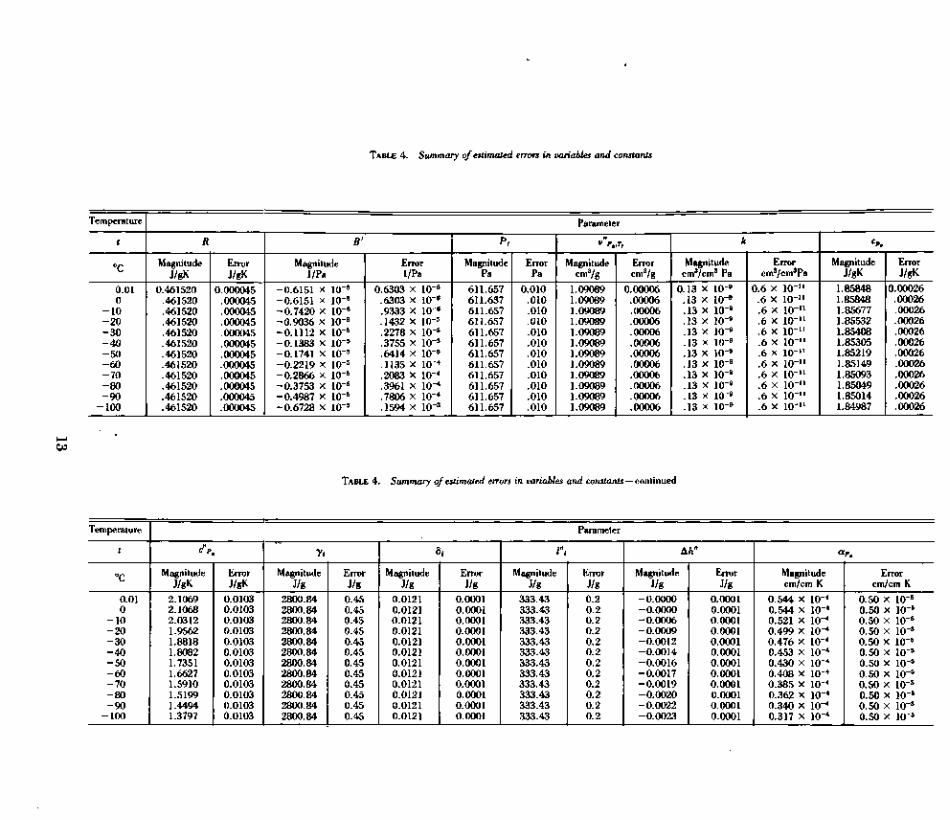
TABLE 4. Summary of estimated errors in variables and constants

Temperature

t

°C

0.010

- 1 0- 2 0- 3 0- 4 0- 5 0- 6 0- 7 0- 8 0- 9 0

-100

Parameter

R

MagnitudeJ/gK

0.461520.461520.461520.461520.461520.461520.461520.461520.461520.461520.461520.461520

ErrorJ/gK

0.000045.000045.000045.000045.000045.000045.000045.000045.000045.000045.000045.000045

B'

MagnitudeI/Pa

-0.6151 x 1O~6

-0.6151 x 10~6

-0.7420 X 10~6

-0.9036 x 10~6

-0.1112 X 10~5

-0.1383 X 10~5

-0.1741 X 10~5

-0.2219 X 10~5

-0.2866 X 10~5

-0.3753 X 10~5

-0.4987 X 10~5

-0.6728 X 10~5

ErrorI/Pa

0.6303 X 10"6

.6303 X 10~6

.9333 X 10"6

.1432 X 10-5

.2278 X 10~5

.3755 X 10~5

.6414 X KT5

.1135 X 10~4

.2083 X 10~4

.3961 X 10~4

.7806 X 10~4

.1594 X 10~3

Pt

MagnitudePa

611.657611.657611.657611.657611.657611.657611.657611.657611.657611.657611.657611.657

ErrorPa

0.010.010.010.010.010.010.010.010.010.010.010.010

V"Pa.Ti

Magnitudecm3/g

1.090891.090891.090891.090891.090891.090891.090891.090891.090891.090891.090891.09089

Errorcm3/g

0.00006.00006.00006.00006.00006.00006.00006.00006.00006.00006.00006.00006

k

Magnitudecm3/cm3 Pa

0.13 X 10~9

.13 X 10~9

.13 X 10"9

.13 X 10-9

.13 X 10"9

.13 X 10-9

.13 X 10~9

.13 X HT9

.13 X KT9

.13 x 10-9

.13 X 10~9

.13 x 10~9

Errorcm3/cm3Pa

0.6 X 10"1

.6 X 10"1

.6 X HT1

.6 X 10-1

.6 X 10"1

.6 X 10"1

.6 X 10-1

.6 X lO"1

.6 X 10"1

.6 X 10"1

.6 X 10"1

.6 X 10"1

MagnitudeJ/gK

1.858481.858481.856771.855321.854081.853051.852191.851491.850931.850491.850141.84987

ErrorJ/gK

0.00026.00026.00026.00026.00026.00026.00026.00026.00026.00026.00026.00026

TABLE 4. Summary of estimated errors in variables and constants — continued

Temperature

t

°C

0.010

- 1 0- 2 0- 3 0- 4 0- 5 0- 6 0- 7 0- 8 0- 9 0

-100

C"P0

MagnitudeJ/gK

2.10692.10682.03121.95621.88181.80821.73511.66271.59101.51991.44941.3797

ErrorJ/gK

0.01030.01030.01030.01030.01030.01030.01030.01030.01030.01030.01030.0103

7i

MagnitudeJ/g

2800.842800.842800.842800.842800.842800.842800.842800.842800.842800.842800.842800.84

ErrorJ/g

0.450.450.450.450.450.450.450.450.450.450.450.45

MagnitudeJ/g

0.01210.01210.01210.01210.01210.01210.01210.01210.01210.01210.01210.0121

ErrorJ/g

0.00010.00010.00010.00010.00010.00010.00010.00010.00010.00010.00010.0001

Parameter

l"i

MagnitudeJ/g

333.43333.43333.43333.43333.43333.43333.43333.43333.43333.43333.43333.43

ErrorJ/g0.20.20.20.20.20.20.20.20.20.20.20.2

A/i"

MagnitudeJ/g

-0.0000-0.0000-0.0006-0.0009-0.0012-0.0014-0.0016-0.0017-0.0019-0.0020-0.0022-0.0023

ErrorJ/g

0.00010.00010.00010.00010.00010.00010.00010.00010.00010.00010.00010.0001

"Pa

Magnitudecm/cm K

0.544 X 10"4

0.544 X 10-0.521 X 10-'0.499 x 10"'0.476 x 10""0.453 X 10"'0.430 x i (T0.408 X 10-'0.385 x 10~4

0.362 x 10-'0.340 x 10-'0.317 x 10-'

i

i

Errorcm/cm K

0.50 X 10~5

0.50 X 10-5

0.50 X 10~5

0.50 X 10-5

0.50 X 10~5

0.50 X 10~5

0.50 X 10~5

0.50 x 10-5

0.50 X 10~5

0.50 x 10~5

0.50 X 10-5

0.50 x 10"5

TABLE 5. Summary of equivalent errors in vapor pressure due to estimated errors in variables and constants

Temperature

t

°C

0.010

- 1 0- 2 0- 3 0- 4 0- 5 0- 6 0- 7 0- 8 0- 9 0

-100

Parameter

R B' Pt k CPo l"i Ah"

Estimated error in vapor pressure due to estimated error in indicated parameter, ppm

00

83173270376491618756909

10781278

00

532950

12891580184521012363264129433279

161616161616161616161616

< 1< 1< 1< 1< 1< 1< 1< 1< 1< 1< 1

< 1

< 1< 1< 1< 1< 1< 1< 1< 1< 1< 1< 1

< 1

000137

121827385272

00

1566

157295488746

1081150820432708

00

135282440612799

10041229147717522055

< 1< 1< 1< 1< 1< 1< 1< 1< 1< 1< 1

< 1

00

60125195272355436546656778912

< 1< 1< 1< 1< 1< 1< 1< 1< 1< 1< 1

< 1

"Pa

< 1< 1< 1< 1< 1< 1< 1< 1< 1< 1< 1

< 1

EstimatedOverallError0

ppm

1616

559101614111781215625613022356240644978

Square root of the sum of the squares of the estimated errors contributed by each parameter.

4. Comparisons

The first experimental values of the vapor pressure of icewere reported by Regnault [50] in 1847. Subsequently, mea-surements were made by Fischer [51], Juhlin [52], andMarvin [53]. In 1909, Scheel and Heuse [54] at the Physikal-isch-Technische Reichsanstalt (PTR) published the results oftheir work which superseded all earlier determinations forrange, precision and accuracy. Using a Rayleigh inclinedmanometer and a platinum resistance thermometer they mea-sured the vapor pressure from 0 to — 67 °C. In a second paper[55] they suggested that temperatures interpolated from theCallendar formula would be more in accord with the thermo-dynamic scale than the temperatures given in their firstpaper. In 1919, the PTR issued revised values of the Scheeland Heuse measurements [56]. Although not explicitlystated, these new values appear to have been based on theuse of the Callendar formula for interpolating temperaturemeasurements with platinum resistance thermometers.

Weber [57] in 1915, employing both a hot-wire manometerand a Knudsen radiometer, made measurements from —22 to— 98 °C. A limited number of determinations were made byNernst [58] in 1909 and by Drucker, Jimeno, and Kangro[59] in 1915. Douslin and McCullough [60] in 1963, using aninclined dead-weight piston gage, made measurements to— 30 °C. Jancso, Pupezin, and Van Hook [61] in 1970 used adifferential capacitance manometer to effect a series of deter-minations to —78 °C. They used the vapor pressure of ice at0 °C as the reference pressure for their manometer, assigningto it the value 4.581 mm Hg (610.7 Pa).

A comparison of eq (54) with these measurements, exclud-ing the early work of Regnault, Fischer, Juhlin, and Marvin,is shown in figure 1. The temperatures given by the investiga-tors were converted to IPTS-68 for this comparison. Many ofthe errors associated with these measurements are not givenexplicitly so it is difficult to determine both their sources andmagnitudes. Therefore, no attempt has been made to assignuncertainties nor to make corrections except for the tempera-ture scale and, where noted, for reference pressure. Becausethe Jancso, Pupezin and Van Hook pressure measurementswere made with respect to the vapor pressure at the ice pointthey were adjusted to conform to the vapor pressure at 0 °C

predicted by eq (54), namely, 611.154 Pa rather than 610.7Pa (4.581 mm Hg) which Jancso, Pupezin, and Van Hookused.

The sets of data of some of the investigators tend to deviatefrom eq (54) in consistent ways. The Scheel and Heusemeasurements (black dots) are generally lower in magnitude(except for two points) than the vapor pressures calculatedfrom eq (54); the differences increase until at —67 °C theyare of the order of 70 percent. Weber's measurements(pluses) are much closer, but they also are lower in magni-tude (except for two points); at about —98 °C, where supris-ingly Weber obtained several measurements, the deviationsare as large as 25 percent. Among all the investigators, thebest agreement is achieved with Weber. However, Webermade no measurements above —22 °C.

Of the three measurements of Nernst (black squares) two(at —30 and —50 °C) show positive differences and the third(at —40 °C) a negative difference, none exceeding 2 percent.The Drucker, Jimeno, and Kangro measurements (black tri-angles) tend to be high, with one value (at —34 °C) differingby as much as +12.3 percent. The differences for theDouslin and McCullough measurements (asterisks), whichcover the range of temperature from —2 to —31.4 °C, arealmost equally positive and negative in number and reach amagnitude of about one percent at —31.4 °C. The Jancso,Pupezin, and Van Hook differences (circles) scatter more orless randomly in the temperature region above —15 °C; from— 35 °C and below, the differences are all positive, reachinga magnitude of 20 percent at about —78 °C.

The differences far exceed the estimated uncertainty of thevalues predicted by eq (54). It may be inferred from thedifference patterns displayed by these several sets of datathat there are significant systematic errors present in each ofthese data. The obvious conclusion is that a definitive set ofmeasurements remains to be made.

Numerous empirical equations have been proposed to rep-resent the vapor pressure of ice. Scheel and Heuse [54] andThiesen [62] derived formulas which fit the original Scheeland Heuse data [54]. The equations of Tetens [63] andErdelyszky as given by Sonntag [64], are of the Magnus type[65] with different sets of coefficients. The Jancso, Pupezin,and Van Hook [61] empirical equation is based on a leastsquare fit to their own measurements.

14

S

S

DU

40

20

0

-20

-40

-60

an

1

-

-

-

-

1

1 1 1

-

o

•

t

1 1 * 1

o

4

2

0

- 2

-4

-6

Q

-

*

•

•

i

t1

-

*

-

-

i

U.D

0.4

0.2

0.0

- 0 .2

-0 .4

-0 .6

n ft

-

- #

— oo

_ o

o°i

o

-

- •

1

-

-

4>.o8--• **~

o —•

•

-

1

-100 - 9 0 - 8 0 -70 - 6 0 - 5 0 - 5 0 - 4 0 - 3 0

TEMPERATURE, DEGREES CELSIUS

-20 - 2 0 -10

Relat

FIGURE 1. Comparision with vapor pressure measurements.X 100 between measurement and eq (54) in percent: • Scheel and Heuse; + Weber;

Jive vapor pressure difference

L eq (54) JI Nernst; A Drucker, Jimeno and Kangro; * Douslin and McCullough; O Jancso, Pupezin and Van Hook.

There also have been repeated attempts to derive thermo-dynamically based expressions for the vapor pressure of ice.The equations of Nernst [58], Washburn [66], Whipple [67],and Goff and Gratch [68, 69] were obtained by integrating theClausius-Clapeyron equation and inserting selected values ofthermal data. Vapor pressures based on the Nernst equationwere included in an early edition of the Smithsonian Meteoro-logical Tables [70]. Vapor pressures based on the Washburnequation are given in several standard references [71, 72]often used by chemists. The Goff formulation is used in themeteorological and air conditioning disciplines [73-75]. Theequation ascribed to Kelley [76] is based on an expression hederived for the free energy difference which, when integratedwith respect to temperature, yields the logarithm of the vaporpressure. This equation is given in a widely used set ofGerman tables [77] and by Dushman [78]. The equations ofMiller [79] and Jancso, Pupezin, and Van Hook [61] werederived from an expression for the vaporization process givenin terms of vapor fugacity and condensed phase activity [80].The Miller equation was not presented in explicit form al-though calculated vapor pressures were given in an abbrevi-ated table.

A comparison between the empirical equations and eq (54)is shown in figure 2 and a similar comparison between thethermodynamic equations and eq (54) is shown in figure 3.Because the Thiesen and the Whipple equations give func-tional relationships for the ratio p/po, where p is the vaporpressure at any given temperature and p0 is the vapor pres-sure at 0 °C, the value predicted by eq (54) was inserted forp0to compute p rather than the value used by these investiga-tors. No attempt was made to adjust or correct any of theempirical equations from the temperature scale used by theinvestigator in his formulation to IPTS-68.

3 -

2 -

0 -

fi -1 -

-2 -

-3 -

-5 -

-6

1 \ 1

1 1

- /

1

1

SCHEEL AND

ERDELYSZK

1 1

HEUSE

JANCSO ET AL

•

THIESEN /

/ /

1 //I

1

f/1

1 1 1

>

yTETENS

1 1

1

—

-

-

-100 -90 -80 -70 -60 -50 -40 -30

TEMPERATURE. DEGREES CELSIUS

- 2 0 -10

FIGURE 2. Comparison with empirical equations.Relative vapor pressure difference ~r X 100 between empirical equation c

L eq (54) jthe literature and eq (54) in percent.

15

-

KELLEY

JANCSO ET AL

-

GOFF AND GRATCH

WHIPPLE / //

/

i i i i i

i i i i i

i i

-

-

- 3 -

-5

-100 - 9 0 - 8 0 - 7 0 - 6 0 - 5 0 - 4 0 - 3 0 - 2 0 -10

TEMPERATURE. DEGREES CELSIUS

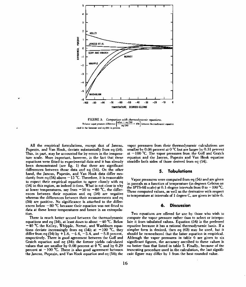
FIGURE 3. Comparison with thermodynamic equations.Relative vapor pressure difference

"other - eq (54)

cited in the literature and eq (54) in percent.eq(54)

X 100 between thermodynamic equation

All the empirical formulations, except that of Jancso,Pupezin, and Van Hook, deviate substantially from eq (54).This, in part, may be accounted for by errors in the tempera-ture scale. More important, however, is the fact that theseequations were fitted to experimental data and it has alreadybeen demonstrated (see fig. 1) that there are significantdifferences between those data and eq (54). On the otherhand, the Jancso, Pupezin, and Van Hook data differ ran-domly from eq (54) above —15 °C. Therefore, it is reasonableto expect their empirical equation to agree closely with eq(54) in this region, as indeed it does. What is not clear is whyat lower temperatures, say from —50 to —80 °C, the differ-ences between their equation and eq (54) are negativewhereas the differences between their measurements and eq(54) are positive. No significance is attached to the differ-ences below —80 °C because their equation was not fitted todata at these lower temperatures and hence is an extrapola-tion.

There is much better accord between the thermodynamicequations and eq (54), at least down to about —40 °C. Below— 40 °C the Kelley, Whipple, Nernst, and Washburn equa-tions deviate increasingly from eq (54); at —100 °C, theydiffer from eq (54) by +1.6, —4.4, —5.4, and —5.8 percent,respectively. There is good agreement between the Goff andGratch equation and eq (54); the former yields calculatedvalues that are smaller by 0.08 percent at 0 °C and by 0.29percent at —100 °C. There is also good agreement betweenthe Jancso, Pupezin, and Van Hook equation and eq (54); the

vapor pressures from their thermodynamic calculations aresmaller by 0.06 percent at 0 °C but are larger by 0.31 percentat —100 °C. The vapor pressures from the Goff and Gratchequation and the Jancso, Pupezin and Van Hook equationstraddle both sides of those derived from eq (54).

5. Tabulations

Vapor pressures were computed from eq (54) and are givenin pascals as a function of temperature (in degrees Celsius onthe IPTS-68 scale) at 0.1-degree intervals from 0 to -100 °C.These computed values, as well as the derivative with respectto temperature at intervals of 1 degree C, are given in table 6.

6. Discussion

Two equations are offered for use by those who wish tocompute the vapor pressure rather than to select or interpo-late it from tabulated values. Equation (54) is the preferredequation because it has a rational thermodynamic basis. If asimpler form is desired, then eq (63) may be used, but itshould be remembered that the latter equation is empirical.Although the vapor pressures in table 6 are given to sixsignificant figures, the accuracy ascribed to these values isno better than that listed in table 5. Finally, because of thetruncating procedure used in the calculation, the last signifi-cant figure may differ by 1 from the best rounded value.

16

) .—i co © h- c

© O

\OOh^Tt^ r - 1 , — i ON CO

Ni—' 0 0 CM © TJ«

lOOMOHNHHHHHH

00

drJC0O(N^N j H 10 O CO O t>

5 00 i—t lO © LO r—i h-

5'iO LO rt "* CO CO CM

iO^H>O0>* )H00NcomiOt^COiO'

) (N 00-N X ^^ H t t ^ O

HNi0(NONr0N0NHC0^l0\rHC lOO

|3

!

I

VO

dHiCC0NC0i

i CM CM L O i—i © <—i r t C5 ON l O -—t 0 0 i O CM ON v

a; 5 l O LO O N CM m C ) <—• 0 0 CO> T f CM LO

COLOVOCSJC > V1L0L0 I -Hi O 0 0 H

CO r"^ Li—iTf(N(| ~ ~ | C 0 ' - 0 L0O^

( N H H H H H t

) o \o a ^ o t5 l O CM ON r - i O C5 CO CO ( N <N <N (,

©fo t-co0 0 CO ON CO

J 3 © S CM t^ C 5SSS5HvOCOC

MOMn(NOMOMHO\^O^W(NHOT t C O C O C O C O C M C M C M C M r H i — l i — I r H i — l i — I r — I r H

H^ONPCOON©^

. . ss^H rf 00 CM h- CO ON

^H ON 00 t^ vO* vd LO Tt rf CO CO* CM

r - CO CO LO <^^ in i H

'* <—• LO C

2 CM VO C 50HCOO^^CO3OSCOrOINWCOLCiONHNiOtOvOONCO^iOCOlNlNfN^OONINvOHvOHNCOON^INi^Nin^^HOt)ir5HN«0>€C0O00lOC0-HO\NV0^'C0(NHO0>00NO^0L0lO^('*«C0CCM(N(NrHrHrHrHrHHrHj L O L O T f < ^ ' C O C O C O C O C M C M C M C M ' — I —Ir -1 r—Ir-1 i—I !-H —H

M.-—i ©ONCOr^OLOiOTfrococo

JfOr-i| I I | I I I

I I Ir-1 CM.CO ' t iOONCOONOHfqcO^inONOOONOHMCOTtiO'OhCOONC'- 'CM(N(NC<llN(NC<l^(N(NrOirOfO«W«COcr:cO«T}<rf'rJ lTtTj<^Tt^ l '3'rtini/:in

I I I I I I I I I I I I I I I I I I I I I I I I I I I I I I I I

17

CMf—ir-iOLOLOOCOiOrf<OCOrtCMOLO

H H i N H ^ O i O O l N M O ^ ^ C O H l Ni O O O 0 O 0 O W O N f j O M

^^

03 O H rH CM O CO

83!)NfOC0cOrHG\HfON^>CMrHCMLO00rH00ON00<

O O i 23! .3 LO O iN r—I ON r

5 ON CO "^ CM r-H O C5 CM CM ON CO CM O C~ ') cO co *O ^^ ^* cO t _

CM CM '

OO MCO^NHiOOO(Nt^OLOTf*rtCOCOCMCM

.(NHHOlOHOHNNTtHlO"

• CO CO O CM < 3S:

3 CM CO CO ^^ ^ * ON CO ^D *O ON CM ^^ CO tmm^ ^^ CM Ni | ~ H O N r — I L O C M C O O O C O C O C O O N O N C O L O O '

OOLOr^ONCMOOCMcOCMOCOOOOOONOOCMLOOrfCO

coO1—^L O r H O

CM^'

1 CM 1^ ON CM CO CO C5 LO CO "^ O CO O LO5 lO ON IS- t^ Is*- O CMN ON O CO t~^" CM CO LO

CM CM —I r-H r-H r-l r-H

vO

NOOOcOOOOrH) O N O O L O L O L O I - H^ ^* ^* O t CM r™ LO CM ^ * r" C

t O H C 0 t O

O ^ O M O i O Or^ cO ON CO CO CM CO CM

' ^ ' O 0 ^ H ^ l O H H

cd PH0 ^

5 O t- r-H r-H LO L)NrthH\Oi5 LO r-H rf. CO Tj" t 5 ^H O N "<* rt O N <

5 h- O N Tf CO CO C

3 t^ r-H CM C

ca 0-OH S

? CO LO O N r-H O N C 5 SO O LO ^N CM LO CO V5 CO t^ CO i

LO CM C^* O N CO CO D ON N

CM O N CM L O L O O N C < r-H r-H CO LO LO CO

OCMr-COCMC -,COCMr-HCO^OOO^LOvN^mt^ONiMfO'tc

CMCMCMr-Hi-Hr-HrHr-Hv,

LO 00 O 1^ r-H5 005 LO

Nr-H|^OOOLOr-HrtTtOOCOrHCOCOr-HOCOCMCO^COCMl^CMONOCOr-HONr^OLOTf<COCOCMCMrHOONOCMLOONTtONLOr—lCOOCOr-HOCOt^OLOTf*COCOCMCMr-Hr—Ir-Hr-H

>r^OOONLOCMrtrHONMONOOJO^OMiOMNiONHLO'N"COO^LOONLO^LOr^OLOO

^ Si- . w. . , . O W Cl O N H i O H N r f

CO CM CM r-H r-^

CO ^ * L O ^O t ** 00 ^ N C^' ^^ C

- I I 1 I I I I I I I I I I I I I I I I I I I I I I I I I I I I I I I I I I I I I I I I I I

18

7. References

[1] Wexler, A., and Greenspan, L., Vapor pressure equation for water inthe range 0 to 100 °C, J. Res. Nat. Bur. Stamd. (U.S.), 75A (Physand Chem.), No.3, 213-230 (May-June 1971).

[2] Stimson, H. F., Some precise measurements of the vapor pressure ofwater in the range from 25 to 100 °C, Nat. Bur. Stand. (U.S.), 73A(Phys. and Chem.), No. 5, 493-496 (Sept.-Oct. 1969).

[3] Wexler, A., Vapor pressure equation for water in the range 0 to 100 °C.A revision, J. Res. Nat. Bur. Stand. (U.S.), 80A (Phys. andChem.), No. 5, (Sept.-Oct. 1976).

[4] Guildner, L., Johnson, D. P., and Jones, F. E., Vapor pressure ofwater at its triple point, Nat. Bur. Stand. (U.S.), 80A, (Phys. andChem.), No. 3, 505-521 (May-June 1976).

[5] Guildner, L. and Edsinger, R. E., Deviation of international practicaltemperatures from thermodynamic temperatures in the temperaturerange from 273.16K to 730 K, J. Res. Nat. Bur. Stand. (U.S.), 80A(Phys. and Chem.), No. 5, 703- (Sept.-Oct. 1976).

[6] The international practical temperature scale of 1968, Metrologia 5, 35(1969).

[7] Burgess, G. K., The international temperature scale, J. Res. Nat. Bur.Stand. (U.S.), 1, 635-640 (1928) RP22.

[8] Stimson, H. F., International temperature scale of 1948, J. Res. Nat.Bur. Stand. (U.S.), 4 2 , 209-217 (1949) RP1962.

[9] Stimson, H. F., International practical temperature scale of 1948. Textrevision of 1960. J. Res. Nat. Bur. Stand. (U.S.), 65A (Phys. andChem.), No. 3, 139-145 (1961).

[10] Douglas, T. B., Conversion of existing calorimetrically determinedthermodynamic properties to the basis of the international practicaltemperature scale of 1968, J. Res. Nat. Bur. Stand. (U.S.), 73A(Phys. and Chem.), No. 5, 451-470 (Sept.-Oct. 1969).

[11] Riddle, J. L., Furukawa, G. T., and Plumb, H. H., Platinum resist-ance thermometry, NBS Monograph 126, Supt. of Documents, Gov-ernment Printing Office, Washington, D. C. 20402, (April 1973).

[12] Goff, J. A., and Gratch, S., Thermodynamic properties of moist air,Heating, Piping and Air Conditioning, ASHVE Journal Section 17,334 (1945).

[13] Goff, J. A., and Gratch, S., Low-pressure properties of water from-160 to 212 F, Trans. ASHVE 52 , 95 (1946).

[14] Goff, J. A., Standardization of thermodynamic properties of moist air,Heating, Piping and Air Conditioning, ASHVE Journal Section 21 ,118(1949).

[15] Keyes, F. G., The thermodynamic properties of water substance 0° to150°C, J. Chem. Phys. 15, 602 (1947).

[16] Keenan, J. H., Keyes, F. G., Hill, P. G., and Moore, J. G., SteamTables (John Wiley & Sons, Inc., New York, 1969).

[17] Bain, R. W., Steam Tables, 1964 (Her Majesty's Stationery Office,Edinburgh, 1964).

[18] Dorsey, N. E., Properties of Ordinary Water-substance (Reinhold Pub.Corp., New York, 1940).

[19] Ginnings, D. C , and Corruccini, R. J., An improved ice calorimeter —the determination of its calibration factor and the density of ice at 0°C, J. Res. Nat. Bur. Stand. (U.S.), 38, 583-591 (1947) RP1796.

[20], Jakob, M., and Erk, S., Warmedehnung des Eises zwischen 0 und-253°, Wiss. Abh. Physik.-Techn. Reichsanst. 12, 301 (1928-29).

[21] Powell, R. W., Preliminary measurements of the thermal conductivityand expansion of ice, Proc. Roy. Soc. A247, 464 (1958).

[22] Butkovich, T. R., Thermal expansion of ice, J. App. Phys. 30 , 350(1959).

[23] Dantl, Gerhard, Warmeausdehnung von H2O- und D2O-Einkristallen,Z. fur Phys. 166, 115 (1962).

[24] LaPlaca, S. and Post, B., Thermal expansion of ice, Acta Cryst. 13,503 (1960).

[25] Judson, L. V., Units of weight and measure. Definitions and tables ofequivalents, NBS Misc. Pub. M214, (1955), U. S. Gov't PrintingOffice, Washington, D. C.

[26] Zemansky, M. W., Heat and Thermodynamic (McGraw-Hill, NewYork, 1951).

[27] Leadbetter, A. J., The thermodynamic and vibrational properties ofH2O ice and D2O ice, Proc. Roy. Soc. A287, 403 (1965).

[28] Nernst, W., Koref, F., and Lindemann, F. A., Untersuchungen iiberdie specifische Warme bei tiefen Temperaturen, Sitz. Akad. Wiss.Berlin 3 , 247 (1910).

[29] Pollitzer, F., Bestimmung spezifischer Warmen bei tiefen Temperatu-ren und ihre Verwertung zur Berechnung elektromotorischer Krafte,Zeit. far Elektrochemie 17, 5 (1911); 19, 513 (1913).

[30] Dickinson, H. C , and Osborne, N. S., Specific heat and heat of fusionof ice, Bull. Bur. Stds. 12, 49 (1915).

[31] Maass, 0., and Waldbauer, L. J., The specific heats and latent heats offusion of ice and of several organic compounds, J.' Amer. Chem.Soc. 47 , 1 (1925).

[32] Barnes, W. H., and Maass, 0., Specific heats and latent heat of fusionof ice, Can. J. Res. 3 , 205 (1930).

[33] Barnes, W. H., and Maass, 0. , A new adiabatic calorimeter, Can. J.Res. 3 , 70 (1930).

[34] Giauque, W. F., and Stout, J. W., The entropy and the third law ofthermodynamics. The heat capacity of ice from 15 to 273 °K, J.Amer. Chem. Soc. 58, 1144(1936).

[35] Sugisaki, M., Suga, H., and Seki, S., Calorimetric study of the glassystate. IV. Heat capacities of glassy water and cubic ice, Bull. Chem.Soc. Japan 4 1 , 2591 (1968).

[36] Osborne, N. S., Heat of fusion of ice. A revision, J. Res. Nat. Bur.Stand. (U.S.), 23, 643-646 (1939) RP1260.

[37] Friedman, A. S., and Haar, L., High-speed machine computation ofideal gas thermodynamic functions. I. Isotopic water molecules, J.Chem. Phys. 22 , 2051 (1954).

[38] Osborne, N. S., Calorimetry of a fluid, J. Res. Nat. Bur. Stand. (U.S.),4 , 609-629 (1930) RP168.

[39] Fiock, E. F., and Ginnings, D. C , Heat of vaporization of water at 50°,70° and 90°C, J. Res. Nat. Bur. Stand. (U.S.), 8, 321-324 (1932)RP416.

[40] Osborne, N. S., Stimson, H. F., and Ginnings, D. C , Calorimetricdetermination of the thermodynamic properties of saturated water inboth the liquid and gaseous states from 100° to 374 °C, J. Res. Nat.Bur. Stand. (U.S.), 18, 389-431 (1937) RP983.

[41] Osborne, N. S., Stimson, H. F., and Ginnings, D. C , Measurementsof heat capacity and heat of vaporization of water in the range 0° to100°C, J. Res. Nat. Bur. Stand. (U.S.), 2 3 , 197-260 (1939)RP1228.

[42] Kell, G. S., Precise representation of volume properties of water at oneatmosphere, J. Chem. Eng. Data 12, 66 (1967).

[43] Cohen, E. R. and Taylor, B. N., Fundamental physical constants, J.Phys. Chem. Ref. Data 2 , 663 (1973).

[44] Eisenberg, D. and Kauzman, W., The Structure of Water, Oxford(University, Press, New York and Oxford, 1969).

[45] Shatenshtein, A. I., Yakovleva, E. A., Zvyagintseva, E. N., Varshav-skii, Ya. M., Israilevich, E. J., and Dykhno, N. M., IsotopicAnalysis of Water, United States Atomic Energy Commission trans-lation AEC-tr-4136 (1960).

[46] International Union of Pure and Applied Chemistry Commission onAtomic Weights, Atomic Weights of the Elements, Pure and Ap-plied Chem. 37, 591-603 (1974).

[47] Abramowitz, M. and Stegun, I. A., Handbook of Mathematical Func-tions, NBS Appl. Math. Ser. 55, 885 (June 1964), U. S. Gov'tPrinting Office, Washington, D. C. 20402.

[48] Natrella, M. G., Experimental Statistics, NBS Handbook 91 (1963), U.5. Gov't Printing Office, Washington, D. C. 20402.

[49] Ku, H. H., Notes on the use of propagation of error formulas, J. Res.Nat. Bur. Stand. (U.S.), 70C (Eng. and Instr.) No. 4, 263-273(Oct.-Dec. 1966).

[50] Regnault, V., Huitieme Memoire. Des forces elastiques de la vapeurd'eau aux differentes temperatures, Memoires de l'Academie desSciences de l'Institut de France, Paris 2 1 , 465 (1947).

[51] Fischer, W., Uber die Tension der iiber flussiger und der iiber festerSubstanz gesattigter Dampfe, Ann. Physik Chem. 28 , 400 (1886).

[52] Juhlin, J., Bestamming of Vattenangangs Maximi-Spangstighet ofver ismellan 0° och —50° Cels samt ofver vattern mellan +20 och — 13°C,Bihang till K. Svenska Vet. - Kad. Handlingar. Stockholm 17, Afd.I. Nr. 1 (1891).

[53] Marvin, C. F., Annual Report of the Chief Signal Officer, AppendixNo. 10, 351-383 (1891).

[54] Scheel, K., and Heuse, W., Bestimmung der Sattigungsdruckes vonWasserdampf unter 0°, Ann. Physik. 29 , 729(1909).

[55] Scheel, K. and Heuse, W., Bestimmung des Sattigungsdruckes von

19

Wasserdampf zwischen 0 und + 50u, Ann. Physik IV 31, 715(1910).

[56] Holborn, L., Scheel, K., and Henning, F., Warmetabellen (Viewegund Sohn, 1919).

[57] Weber, S., Investigation relating to the vapour pressure of ice, Com-munications from the Phys. Lab. Univ. Leiden, No. 150a, (1915).

[58] Nernst, W., Thermodynamische Behandlung einiger Eigenschaften desWassers, Verh. Deut. Physik. Ges. 11 , 313 (1909).

[59] Drucker, C , Jimeno, E., and Kangro, W., Dampfdrucke fliissigerStoffe bei niedrigen Temperaturen, Zeit. Phys. Chem. 90, 513(1915).

[60] Douslin, D. R. and McCullough, J. P., An inclined-piston deadweightpressure gage, U. S. Bureau of Mines Rept. of Investigation No.6149 (1963).

[61] Jancso, G., Pupezin, J., and Van Hook, W. A., The vapor pressure ofice between + 10~2 and -102 0 , J. Phys. Chem. 74, 2984 (1970).

[62] Thiesen, M., Die Dampfspannung iiber Eis, Ann. der Phys. (4)29,1057 (1909).

[63] Tetens, 0., Uber einize meteorologische Begriffe, Zeit. fiir Geophysik6, 297 (1930).

[64] Sonntag, D., Hygrometrie (Akademie-Verlag, Berlin, 1966).[65] Magnus, G., Versuche iiber die Spannkrafte des Wasserdampfes, Ann.

Physik. Chem. (Poggendorff) 6 1 , 225 (1844).[66] Washburn, E. W., The vapor pressure of ice and of water below the

freezing point, Monthly Weather Review 52, 488 (1924).[67] Whipple, F. J. W., Formulae for the vapour pressure of ice and water

below 0°C, Monthly Weather Review 55 , 131 (1927).[68] Goff, J. A., Vapor pressure of ice from 32 to -280 F, Trans. ASHVE

4 8 , 299 (1942).[69] Goff, J. A., Saturation pressure of water on the new kelvin scale. In:

Humidity and Moisture, Vol. I l l , Wexler, A. and Wildhack, W. A.,Eds, 289 (Reinhold Publishing Corp., New York, 1965).

[70] Smithsonian Meteorological Tables, 5th Revised Edition, SmithsonianInstitution, Washington (1931).

[71] International Critical Tables, Vol. 3 (McGraw-Hill, New York, 1928).[72] Handbook of Chemistry and Physics, 46th ed. (Chemical Rubber Pub.

Co., Cleveland, 1965).[73] List, R. J., (ed.) Smithsonian Meteorological Tables, 6th Revised ed.,

Smithsonian Institution, Washington (1951).[74] Letestu, S., Ed., International Meteorological Tables, WMO-No. 188.

TP. 94, World Meteorological Organization, Geneva (1966).[75] ASHRAE Guide and Data Book, Fundamentals and Equipment 1961,

1965 and 1966, America Society of Heating (Refrigerating and AirConditioning Engineers, Inc., New York).

[76] Kelley, K. K., Contributions to the data on theoretical metallurgy, III.The free energies of vaporization and vapor pressures of inorganicsubstances, Bulletin 383, Bureau of Mines, (1935).

[77] Landolt-Bb'rnstein Tabellen, 6 Auflage, II. (Springer-Verlag, Berlin,1960).

[78] Dushman, S., Scientific Foundations of Vacuum Technique, (JohnWiley & Sons, Inc., 1949).

[79] Miller, G. A., Accurate calculation of very low vapor pressures: ice,benzene, and carbon tetrachloride, J. Chem. Eng. Data 7, 353(1962).

[80] Lewis, G. N. and Randall, M., Thermodynamics, revised by Pitzer, K.S., and Brewer, L. B. (McGraw-Hill, New York, 1961).

(Paper 81A1-920)

20