vapor-phase chemical equilibrium and combined … chemical equilibrium and combined chemical and...
TRANSCRIPT

Vapor-phase chemical equilibrium and
combined chemical and vapor-liquid equilibrium
for the ternary system ethylene + water + ethanol
from reaction-ensemble and reactive Gibbs-ensemble
molecular simulations
Y. Mauricio Muñoz-Muñoz a,b, Jadran Vrabecb, Mario Llano-Restrepo a*
a School of Chemical Engineering, Universidad del Valle,
Ciudad Universitaria Melendez, Building 336,
Apartado 25360, Cali, Colombia
b Thermodynamics and Energy Technology,
University of Paderborn, 33098 Paderborn, Germany
* Corresponding author. Tel: + 57-2-3312935; fax: + 57-2-3392335
E-mail address: [email protected] (M. Llano-Restrepo)

2
Abstract
Reliable combined chemical and vapor-liquid equilibrium (ChVLE) data for the ternary system
ethylene + water + ethanol are required for the conceptual design of a reactive separation process
to obtain ethanol by the hydration of ethylene. Due to the absence of experimental data for the
combined ChVLE of the reacting system, molecular simulation looks appealing to predict such
data. In this work, the reaction-ensemble Monte Carlo (RxMC) method was used to calculate the
chemical equilibrium of the ternary system in the vapor phase, and the reactive Gibbs-ensemble
Monte Carlo (RxGEMC) method was used to calculate its combined ChVLE. A set of previously
validated Lennard-Jones plus point-charge potential models were employed for ethylene, water,
and ethanol. The RxMC predictions for the vapor-phase chemical equilibrium composition of the
ternary system and the equilibrium conversion of ethylene to ethanol, at 200°C and pressures of
30, 40, 50, and 60 atm, were found to be in good agreement with predictions made by use of a
previously proposed thermodynamic model that combines the Peng-Robinson-Stryjek-Vera
equation of state, the Wong-Sandler mixing rules, and the UNIQUAC activity coefficient model.
The RxGEMC calculations were used to predict the reactive phase diagram (two-dimensional
graph of pressure versus transformed liquid and vapor-phase ethylene mole fractions) at 200°C.
In contrast to the thermodynamic model, molecular simulation predicts a wider reactive phase
diagram (due to a reactive dew-point line much richer in ethylene). However, these two
independent approaches were found to be in very good agreement with regard to the predicted
bubble-point line of the reactive phase diagram and the approximate location of the reactive
critical point.
Keywords: Chemical equilibrium; reactive phase equilibrium; ternary systems; reactive critical
point; ethylene hydration; petrochemical ethanol.
3
1. Introduction
The concept of process intensification could be applied in the petrochemical industry to the
production of ethanol by the direct hydration of ethylene. In the intensified process, the
simultaneous reaction and separation of the product (ethanol) and the reactants (ethylene and
water) would occur in the same piece of equipment, a reactive separation column, into which
gaseous ethylene and liquid water would be fed [1].
In a previous study [2], we corroborated the validity of a set of previously published Lennard-
Jones plus point-charge potential models for ethylene [3], water [4], and ethanol [5] from the
good agreement of Gibbs-ensemble Monte Carlo (GEMC) molecular simulation results for the
vapor pressure and the VLE phase diagrams of those components with respect to calculations
made by means of the most accurate (reference) multiparameter equations of state currently
available for ethylene [6], water [7], and ethanol [8]. We found that these potential models are
capable of predicting the available VLE phase diagrams of the binary systems ethylene + water
[9] (at 200 and 250°C), ethylene + ethanol [10] (at 150, 170, 190, 200, and 220°C), and ethanol +
water [11] (at 200, 250, 275, and 300°C). We also found that molecular simulation predictions
for the VLE phase diagrams of the ternary system ethylene + water + ethanol, at 200°C and
pressures of 30, 40, 50, 60, 80, and 100 atm, are in very good agreement with both the
experimental data [12] and predictions that we had previously made [1] by use of a
thermodynamic model that combines the Peng-Robinson-Stryjek-Vera (PRSV2) equation of state
[13, 14], the Wong-Sandler (WS) mixing rules [15], and the UNIQUAC activity coefficient
model [16]. This agreement between the predictions of two independent methods (molecular
simulation and the thermodynamic model) gave us confidence for the subsequent use of
simulation to predict the combined chemical and vapor-liquid equilibrium (ChVLE) of the
ternary system and check the validity of predictions that we previously made [1] by means of the
thermodynamic model.
The reaction-ensemble Monte Carlo (RxMC) method [17-19] has been used successfully by
several authors for the computation of the chemical equilibrium of some reactions of industrial

4
interest, such as the dimerization of nitric oxide [20-22], the esterification reaction of ethanol and
acetic acid to yield ethyl acetate and water [23], the hydrogenation of benzene to cyclohexane
[24], the synthesis of ammonia [20, 25, 26], and the combined hydrogenation of ethylene and
propylene [27]. A very comprehensive review of the RxMC method and its various applications
has been made by Turner et al. [19]. In this work, the RxMC method was implemented in order
to compute the vapor-phase chemical equilibrium of the ternary system ethylene + water +
ethanol (i.e., for the vapor-phase hydration of ethylene to ethanol) and compare the simulation
predictions with those obtained by means of the PRSV2-WS-UNIQUAC thermodynamic model
described in the first of our previous works [1].
The reactive Gibbs-ensemble Monte Carlo (RxGEMC) method [18, 28, 29] is a combination of
the reaction-ensemble (RxMC) [17-19] and the Gibbs-ensemble (GEMC) [30-37] methods, and
it has already been used for the computation of the combined ChVLE of dimerization and
combination reactions [18, 28] and the etherification reaction of isobutene and methanol to
produce methyl-tert-butyl ether [29]. In this work, the RxGEMC method was implemented in
order to compute the combined ChVLE for the hydration of ethylene to ethanol and compare the
simulation predictions with those previously obtained [1] from the thermodynamic model.
The outline of the paper is as follows. The RxMC and the RxGEMC simulation methods are
described in Sections 2.1 and 2.2, respectively. In Section 3.1, simulation results for the vapor-
phase chemical equilibrium of the hydration reaction are reported, discussed, and compared with
calculations previously carried out [1] by means of the PRSV2-WS-UNIQUAC thermodynamic
model. In Section 3.2, simulation results for the combined ChVLE of the hydration reaction are
reported, discussed, and compared with the predictions previously made [1] by use of the
thermodynamic model.
2. Simulation methods The Lennard-Jones (LJ) plus point-charge intermolecular potential models recently devised by
Weitz and Potoff [3] for ethylene, Huang et al. [4] for water, and Schnabel et al. [5] for ethanol

5
were used to carry out the simulations of the present work. These potential models were
described in detail in our previous simulation study [2], and their validity was corroborated from
the good agreement obtained between our simulation results for the vapor pressure and the VLE
phase diagrams of those pure components [2] and calculations carried out by means of the most
accurate (reference) multiparameter equations of state currently available [6-8]. For all
simulations carried out in the present work, the Lorentz-Berthelot combining rules were used to
calculate the size and energy parameters of the LJ potential for unlike interactions [2].
2.1 Simulation method for the vapor-phase chemical equilibrium
In the reaction-ensemble Monte Carlo (RxMC) method, a single simulation box is used to
simulate the vapor-phase chemical equilibrium of a reversible reaction like the hydration of
ethylene to ethanol:
OHHCOHHC 52242 ↔+
There are three types of random moves for the RxMC method [17-19] when dealing with rigid
molecules: translational displacement and rotation of molecules inside the simulation box, box
volume changes, and reaction steps. The moves are accepted or rejected in accordance with a
particular probability recipe that involves the calculation of the total intermolecular potential
energy change o
t
n
tt UUU −=∆ between the new ( n
tU ) and the old ( o
tU ) configurations. The
molecular displacements and rotations, and the box volume changes are carried out in the same
way as in the NPT-ensemble, with the usual probability formulas for the acceptance or rejection
of those trial moves [38, 39]. For the rotational moves required for water and ethanol, the
orientational displacements followed the scheme [38] that chooses random values for the Euler
angles in the rotation matrix, and employs the internal coordinates of the sites of the molecule [2]
to calculate their simulation-box coordinates. The probability of acceptance for the reaction steps
is given by the expression [17, 19]:
6
+
∆−
= ∏
=
C
i ii
i
B
t
eq
B
rxN
N
Tk
UK
Tk
VPP
1
0
)!(
!exp)(,1min
ζνζ
ζν
(1)
where 0P is the standard-state pressure, V is the volume of the simulation box, Bk is the
Boltzmann constant, T is the absolute temperature, eqK is the chemical equilibrium constant of
the reaction, C is the number of components in the reacting system, ∑=
=C
i
i
1
νν with iν as the
stoichiometric coefficient of component i (positive for products and negative for reactants),
1+=ζ for the reaction in the forward direction, 1−=ζ for the reaction in the backward
direction, iN is the number of molecules of component i before the reaction step is taken, and
tU∆ is the total configurational energy change involved in the reaction step. For the hydration of
ethylene to ethanol, the stoichiometric coefficients are 121 −==νν for ethylene (1) and water
(2), 13 +=ν for ethanol (3), and 1−=ν for the reaction.
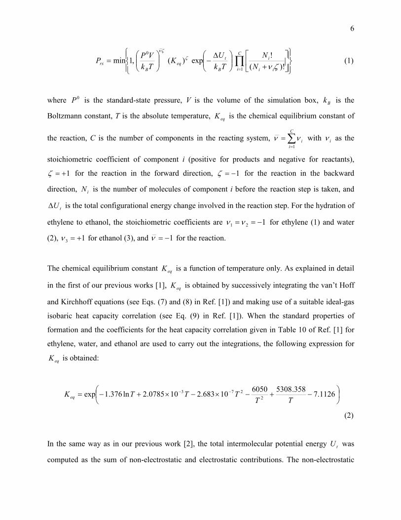
The chemical equilibrium constant eqK is a function of temperature only. As explained in detail
in the first of our previous works [1], eqK is obtained by successively integrating the van’t Hoff
and Kirchhoff equations (see Eqs. (7) and (8) in Ref. [1]) and making use of a suitable ideal-gas
isobaric heat capacity correlation (see Eq. (9) in Ref. [1]). When the standard properties of
formation and the coefficients for the heat capacity correlation given in Table 10 of Ref. [1] for
ethylene, water, and ethanol are used to carry out the integrations, the following expression for
eqK is obtained:
−+−×−×+−= −− 1126.7358.53086050
10683.2100785.2ln376.1exp2
273
TTTTTK eq
(2)
In the same way as in our previous work [2], the total intermolecular potential energy tU was
computed as the sum of non-electrostatic and electrostatic contributions. The non-electrostatic
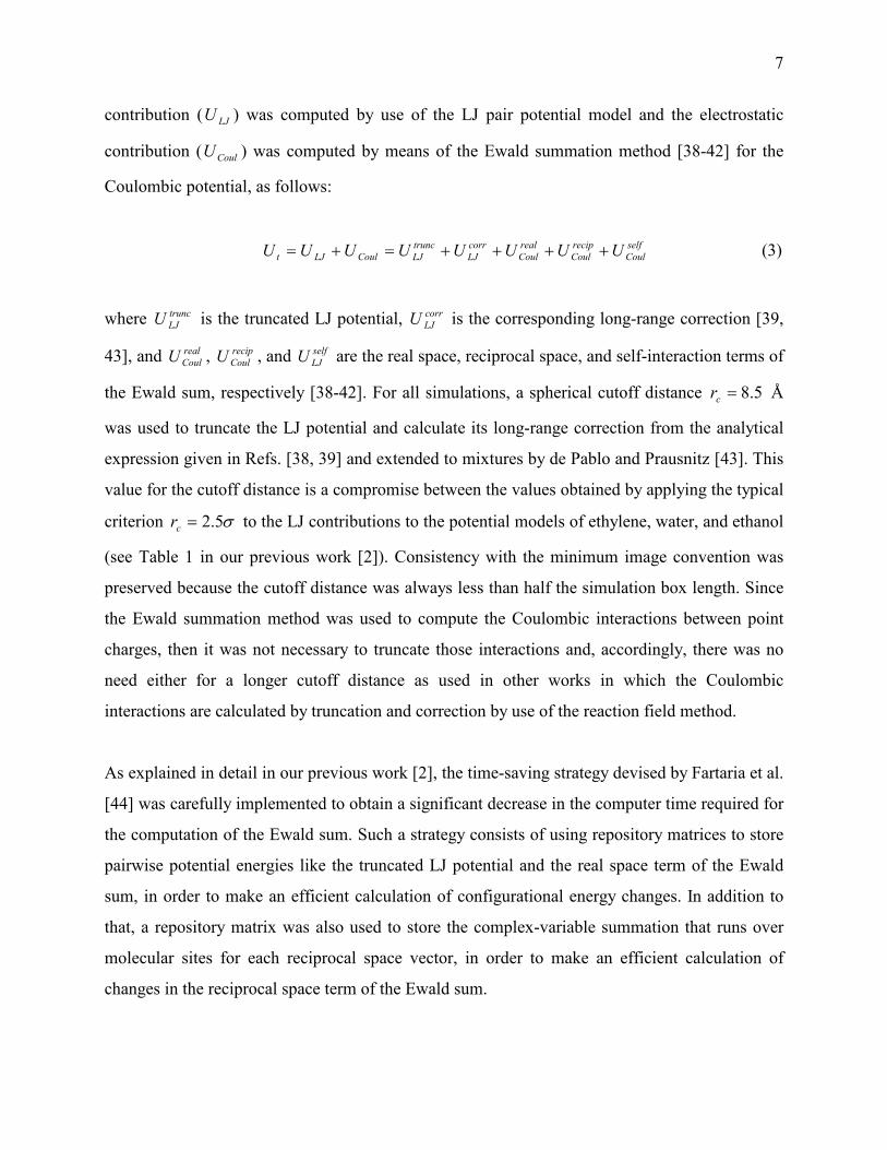
7
contribution ( LJU ) was computed by use of the LJ pair potential model and the electrostatic
contribution ( CoulU ) was computed by means of the Ewald summation method [38-42] for the
Coulombic potential, as follows:
self
Coul
recip
Coul
real
Coul
corr
LJ
trunc
LJCoulLJt UUUUUUUU ++++=+= (3)
where trunc
LJU is the truncated LJ potential, corr
LJU is the corresponding long-range correction [39,
43], and real
CoulU , recip
CoulU , and self
LJU are the real space, reciprocal space, and self-interaction terms of
the Ewald sum, respectively [38-42]. For all simulations, a spherical cutoff distance 5.8=cr Å
was used to truncate the LJ potential and calculate its long-range correction from the analytical
expression given in Refs. [38, 39] and extended to mixtures by de Pablo and Prausnitz [43]. This
value for the cutoff distance is a compromise between the values obtained by applying the typical
criterion σ5.2=cr to the LJ contributions to the potential models of ethylene, water, and ethanol
(see Table 1 in our previous work [2]). Consistency with the minimum image convention was
preserved because the cutoff distance was always less than half the simulation box length. Since
the Ewald summation method was used to compute the Coulombic interactions between point
charges, then it was not necessary to truncate those interactions and, accordingly, there was no
need either for a longer cutoff distance as used in other works in which the Coulombic
interactions are calculated by truncation and correction by use of the reaction field method.
As explained in detail in our previous work [2], the time-saving strategy devised by Fartaria et al.
[44] was carefully implemented to obtain a significant decrease in the computer time required for
the computation of the Ewald sum. Such a strategy consists of using repository matrices to store
pairwise potential energies like the truncated LJ potential and the real space term of the Ewald
sum, in order to make an efficient calculation of configurational energy changes. In addition to
that, a repository matrix was also used to store the complex-variable summation that runs over
molecular sites for each reciprocal space vector, in order to make an efficient calculation of
changes in the reciprocal space term of the Ewald sum.
8
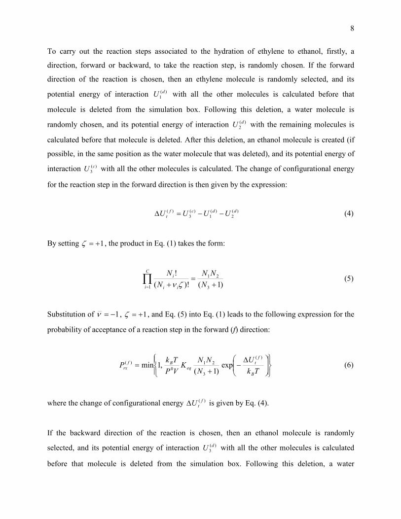
To carry out the reaction steps associated to the hydration of ethylene to ethanol, firstly, a
direction, forward or backward, to take the reaction step, is randomly chosen. If the forward
direction of the reaction is chosen, then an ethylene molecule is randomly selected, and its
potential energy of interaction )(1
dU with all the other molecules is calculated before that
molecule is deleted from the simulation box. Following this deletion, a water molecule is
randomly chosen, and its potential energy of interaction )(2
dU with the remaining molecules is
calculated before that molecule is deleted. After this deletion, an ethanol molecule is created (if
possible, in the same position as the water molecule that was deleted), and its potential energy of
interaction )(3
cU with all the other molecules is calculated. The change of configurational energy
for the reaction step in the forward direction is then given by the expression:
)(2
)(1
)(3
)( ddcf
t UUUU −−=∆ (4)
By setting 1+=ζ , the product in Eq. (1) takes the form:
∏= +
=+
C
i ii
i
N
NN
N
N
1 3
21
)1()!(
!
ζν (5)
Substitution of 1−=ν , 1+=ζ , and Eq. (5) into Eq. (1) leads to the following expression for the
probability of acceptance of a reaction step in the forward (f) direction:
∆−
+=
Tk
U
N
NNK
VP
TkP
B
f
t
eqBf
rx
)(
3
210
)( exp)1(
,1min (6)
where the change of configurational energy )( f
tU∆ is given by Eq. (4).
If the backward direction of the reaction is chosen, then an ethanol molecule is randomly
selected, and its potential energy of interaction )(3
dU with all the other molecules is calculated
before that molecule is deleted from the simulation box. Following this deletion, a water
9
molecule is created (if possible, in the same position as the ethanol molecule that was deleted),
and its potential energy of interaction )(2
cU with all the other molecules is calculated. Next, an
ethylene molecule is created in a random position of the simulation box, and its potential energy
of interaction )(1
cU with all the other molecules is calculated. The change of configurational
energy for the reaction step in the backward direction is then given by the expression:
)(3
)(2
)(1
)( dccb
t UUUU −+=∆ (7)
By setting 1−=ζ , the product in Eq. (1) takes the form:
∏= ++
=+
C
i ii
i
NN
N
N
N
1 21
3
)1)(1()!(
!
ζν (8)
Substitution of 1−=ν , 1−=ζ , and Eq. (8) into Eq. (1) leads to the following expression for the
probability of acceptance of a reaction step in the backward (b) direction:
∆−
++=
Tk
U
NNK
N
Tk
VPP
B
b
t
eqB
b
rx
)(
21
30
)( exp)1)(1(
,1min (9)
where the change of configurational energy )(b
tU∆ is given by Eq. (7).
For the simulation of the vapor-phase chemical equilibrium of the ternary system at given values
of temperature T and pressure P, the following four-stage strategy was implemented. In the first
stage, by specifying the ethylene to water feed mole ratio and defining an initial number of
ethanol molecules in the simulation box equal to zero, the initial numbers of ethylene and water
molecules were defined from a total number of 400 molecules. In the second stage, an NVT-
ensemble simulation (with 400=N molecules) was carried out with an arbitrary vapor-density
value and for a total number of 6101× moves (molecular displacements and rotations), 60 % of
which were used to equilibrate the configurational energy. In the third stage, starting from the

10
final configuration obtained after the NVT run, an NPT-ensemble simulation was carried out for a
total number of 6103× moves (using a ratio of one volume change to N molecular displacements
and rotations), 60% of which were used to equilibrate the density and the configurational energy.
In the fourth stage, starting from the final configuration obtained after the NPT run, a RxMC
simulation (at the fixed conditions of temperature T and pressure P) was carried out for a total
number of 6101× moves, using a ratio of 10 volume changes to N molecular displacements and
rotations and N reaction steps, the latter of which were taken in both directions (forward and
backward) with equal probability. Ensemble averages were computed for the numbers of
molecules of the three components and from these averages, the molar composition of the ternary
system in chemical equilibrium was calculated. Statistical uncertainties (error bars) associated to
the RxMC ensemble-averages were calculated by means of the block averaging method of
Flyvbjerg and Petersen [45].
2.2 Simulation method for the combined chemical and vapor-liquid equilibrium
In the reactive Gibbs-ensemble Monte Carlo (RxGEMC) method [18, 28, 29], two simulation
boxes are used to simulate the combined ChVLE equilibrium of a reversible reaction like the
hydration of ethylene to ethanol. Besides the three types of random moves already explained in
Section 2.1 for the RxMC (i.e., translational displacements and rotations of molecules, box
volume changes, and reaction steps in the forward and backward directions), a fourth move type,
the transfer of molecules between the boxes (i.e., simultaneous deletion and insertion moves) is
performed in order to achieve the phase equilibrium condition of equality of the chemical
potentials in the two phases for each component. The probability formulas for the acceptance or
rejection of this fourth move type have been discussed in several papers on the GEMC method
[30-37] and also in the textbook by Frenkel and Smit [39]. To increase the sampling efficiency,
the reaction steps are usually performed in the vapor phase.
For the simulation of the combined ChVLE of the ternary system, the following four-stage
strategy was implemented. In the first stage, by specifying the temperature T and the pressure P
of the system, estimates of the molar compositions and densities of the coexisting vapor and

11
liquid phases at chemical equilibrium were obtained from a reactive T-P flash calculation with
the help of the PRSV2-WS-UNIQUAC thermodynamic model, as described in detail in the first
of our previous works [1]. In the second stage, for each phase of the mixture, an NVT-ensemble
simulation (with 400=N molecules), with the density and mole fractions fixed at the values
estimated from the thermodynamic model, was carried out for a total number of 7101× moves
(molecular displacements and rotations), 60% of which were used to equilibrate the
configurational energy. In the third stage, starting from the final configuration obtained after the
NVT runs, an NPT-ensemble simulation was carried out for each phase for a total number of
7102× moves (using a ratio of 10 volume changes to N molecular displacements and rotations),
60% of which were used to equilibrate the density and the configurational energy. In the fourth
stage, starting from the final configurations obtained after the NPT runs, a RxGEMC simulation
was carried out for the set of two boxes, for a total number of 7102× moves, using a ratio of 10
volume changes for each box to 2N molecular displacements and rotations, 2N molecular
transfers between the boxes, and 2N reaction steps in the vapor-phase box, the latter of which
were taken in both directions (forward and backward) with equal probability. Properties of the
coexisting phases were sampled every 5105× moves, and running averages were recalculated
until the statistical equality for the chemical potentials of each component in the two phases was
attained. Statistical uncertainties (error bars) associated to the RxGEMC ensemble averages were
also calculated by means of the block averaging method of Flyvbjerg and Petersen [45]. In our
previous simulation work [2], we found that the VLE phase diagram of ethylene + water at
200°C was improved by the use of a correction factor 9.0=χ in the Lorentz combining rule
2/1, )( jiji εεχε = for the energy parameter ijε of the LJ potential for ethylene-water unlike
interactions. That value of the correction factor was also used here to carry out both RxMC and
RxGEMC simulations.
3. Simulation results
3.1 Results for the vapor-phase chemical equilibrium

12
By following the four-stage strategy explained in Section 2.1, RxMC simulations of the vapor-
phase chemical equilibrium for the ternary system ethylene + water + ethanol were carried out at
a temperature of 200°C and pressures of 30, 40, 50, and 60 atm. Simulations were started by
specifying values of the ethylene to water feed mole ratio such that the initial ethylene mole
fraction in the simulation box was in the range from 0.1 to 0.9.
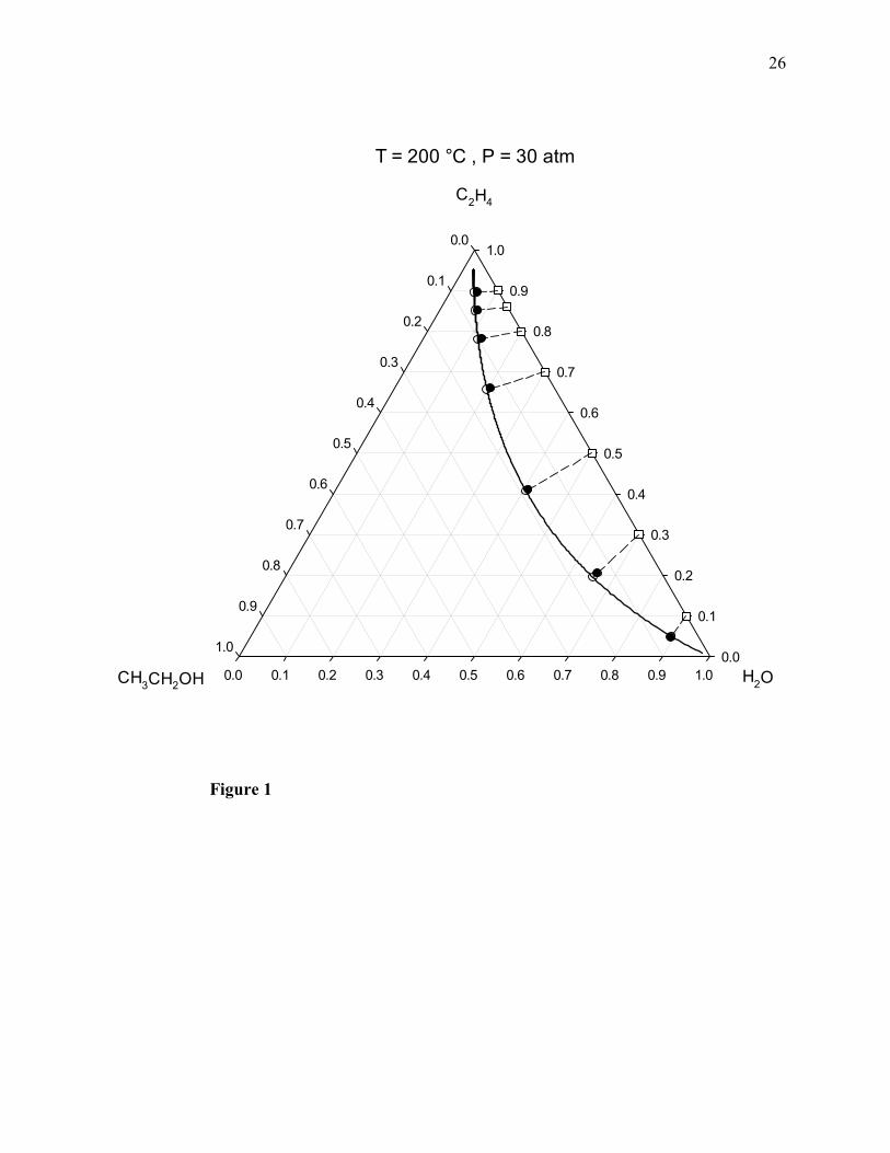
The computed chemical equilibrium molar composition diagrams are shown in Figs. 1-4, where
the filled circles correspond to the molecular simulation results, and both the empty circles and
the solid line correspond to the results obtained by means of the PRSV2-WS-UNIQUAC
thermodynamic model [1]. The dotted lines are used to join the initial (feed) compositions,
marked by the empty squares, and the final (equilibrium) compositions of the ternary system. As
indicated by the longest dotted line in these diagrams, the possible maximum value of the
equilibrium mole fraction of ethanol would correspond to an initial equimolar ethylene + water
mixture, and this maximum mole fraction increases with pressure.
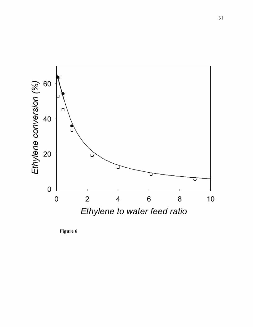
The computed values of the equilibrium conversion of ethylene to ethanol as a funtion of the
ethylene to water feed mole ratio are shown in Figs. 5-8, where the filled circles correspond to
the molecular simulation results, the solid line corresponds to the results obtained from the
thermodynamic model (i.e., for the non-ideal gas mixture), and the empty squares correspond to
the assumption of ideal-gas behavior. As follows from Figs. 5-8, at all pressures, the equilibrium
conversion of ethylene to ethanol decreases with increasing values of the ethylene to water feed
mole ratio. Also, for a given value of the ethylene to water feed mole ratio, the equilibrium
conversion increases with increasing pressure. Simulation predictions for the equilibrium
conversion are in fairly close agreement with the predictions made by use of the thermodynamic
model. The minimum deviation between the simulation predictions and the results from the
thermodynamic model is 1.7% at 30 atm, 1.6% at 40 atm, 2.9% at 50 atm, and 0.6% at 60 atm. In
contrast, results for the equilibrium conversion obtained from the assumption of ideal-gas
behavior for the reacting mixture, exhibit significant deviations at low values of the ethylene to
water feed mole ratio, with respect to both sets of predictions (molecular simulation and
thermodynamic model). The minimum deviation between the ideal gas assumption and the

13
results from the thermodynamic model is 7.8% at 30 atm, 8.7% at 40 atm, 9.0% at 50 atm, and
9.1% at 60 atm.
By means of the thermodynamic model, in the first of our previous works [1], we calculated the
minimum value minr (at the bubble-point) and maximum value maxr (at the dew-point) of the
ethylene to water feed mole ratio r for the existence of two phases at the chemical equilibrium of
the ternary system at 200°C. Those values were reported in Table 12 of Ref. [1]. The ranges
maxmin rrr << (over which the two-phase system occurs) or minrr < (over which a single liquid
phase occurs) can be used to determine whether the conditions chosen to calculate the vapor-
phase chemical equilibrium are valid or not. The values of 0.1, 0.3, 0.5, 0.7, 0.8, 0.86, and 0.9 for
the initial ethylene mole fraction 01y , from which the molecular simulations were started,
correspond to r values of 0.1111, 0.4286, 1.0000, 2.3333, 4.0000, 6.1429, and 9.0000,
respectively. At 30 atm, the thermodynamic model [1] predicts that the two-phase system occurs
for 6977.00575.0 << r ; therefore, the vapor-phase chemical equilibrium compositions shown in
Fig. 1 for values of 0.1 and 0.3 for 01y would be hypothetical, because the reaction would
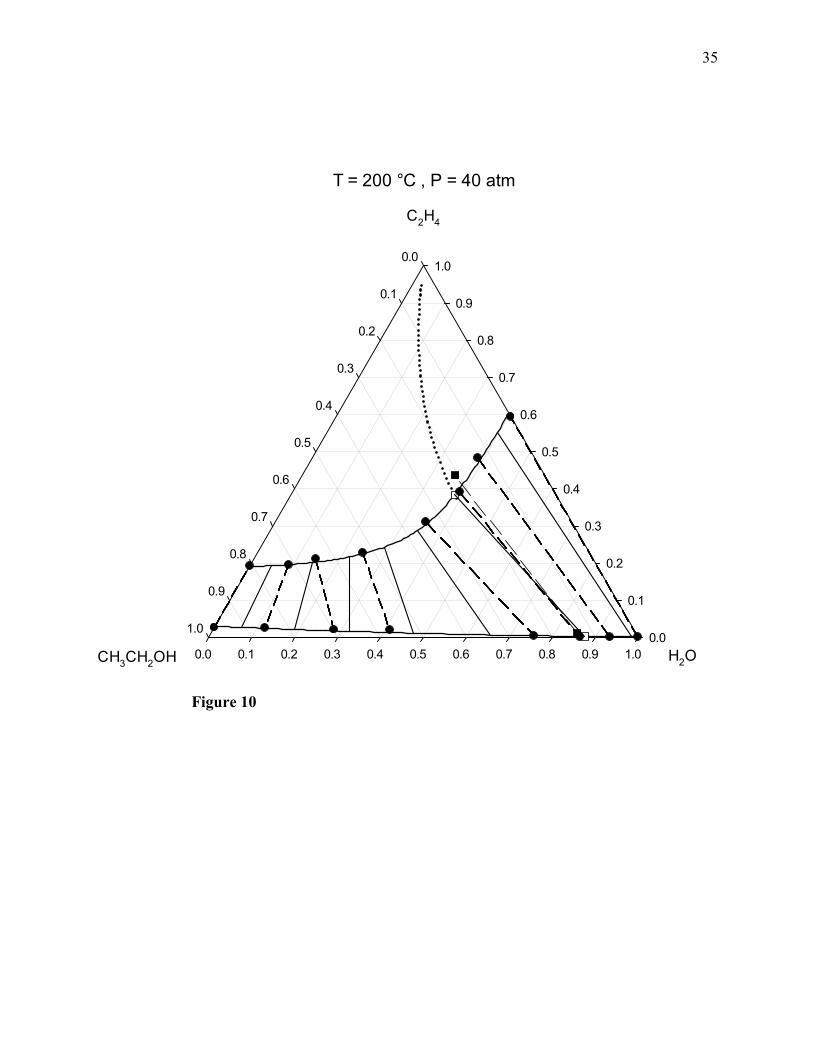
actually occur in a two-phase system. At 40 atm, the thermodynamic model predicts that the two-
phase system occurs for 0030.11262.0 << r and a single liquid phase occurs for 1262.0<r ;
therefore, the vapor-phase chemical equilibrium compositions shown in Fig. 2 for values of 0.1,
0.3, and 0.5 for 01y would also be hypothetical because the reaction would actually occur either
in a single liquid phase (for 1.001 =y ) or in a two-phase system (for 3.00
1 =y and 5.001 =y ). At
50 atm, the thermodynamic model predicts that the two-phase system occurs for
2358.12393.0 << r and a single liquid phase occurs for 2393.0<r ; therefore, the vapor-phase
chemical equilibrium compositions shown in Fig. 3 for values of 0.1, 0.3, and 0.5 for 01y would
also be hypothetical for the same reason given at 40 atm. Finally, at 60 atm, the thermodynamic
model predicts that the two-phase system occurs for 4279.13734.0 << r and a single liquid
phase occurs for 3734.0<r ; therefore, the vapor-phase chemical equilibrium compositions
shown in Fig. 4 for values of 0.1, 0.3, and 0.5 for 01y would also be hypothetical for the same
reason given at 40 and 50 atm.
14
Accordingly, some of the computed values of the vapor-phase equilibrium conversion of ethylene
to ethanol shown in Figs. 5-8 would be hypothetical: the ethylene conversions for r values of
0.1111 and 0.4286 at 30 atm (Fig. 5), and the ethylene conversions for r values of 0.1111,
0.4286, and 1.0000 at 40, 50, and 60 atm (Figs. 6-8).
3.2 Results for the combined chemical and vapor-liquid equilibrium
By following the four-stage strategy explained in Section 2.2, RxGEMC simulations of the
combined ChVLE of the ternary system ethylene + water + ethanol were carried out at a
temperature of 200°C and at 11 values of pressure. The resulting phase diagrams are shown in
Figs. 9-14 (at 30, 40, 50, 60, 80, and 100 atm) and Figs. S1-S5 (at 70, 90, 110, 130, and 150
atm), the latter of which are reported as Supplementary data in Appendix A.
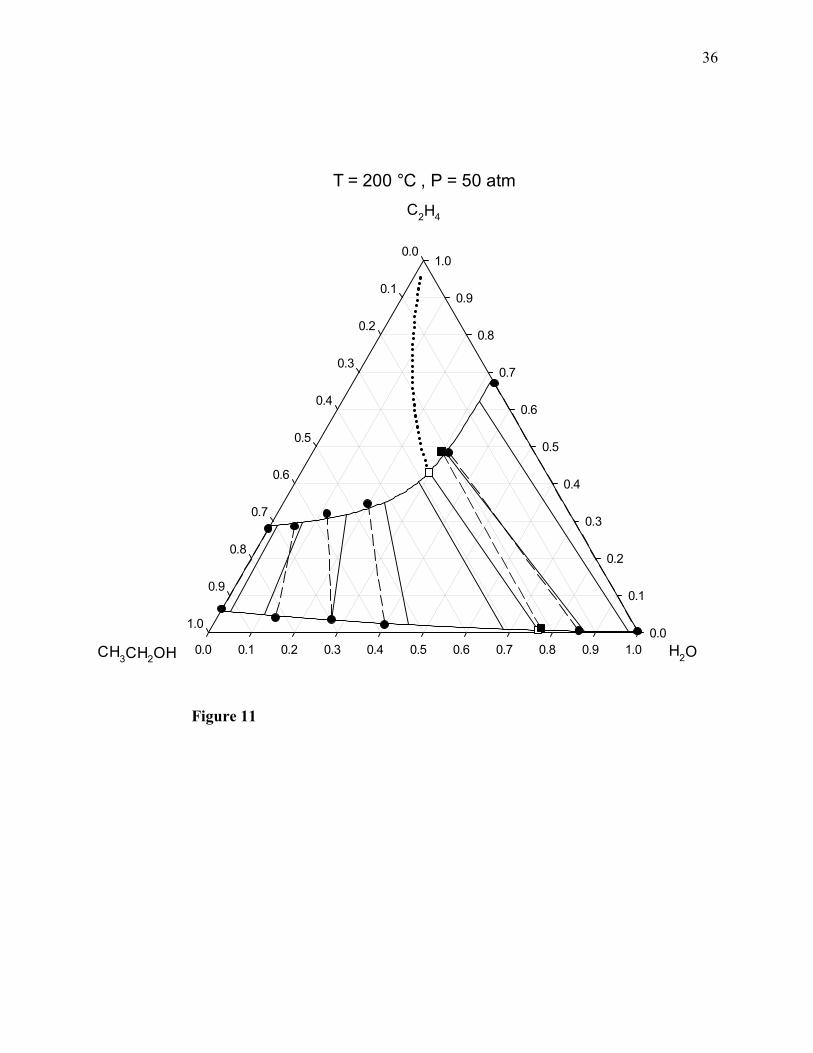
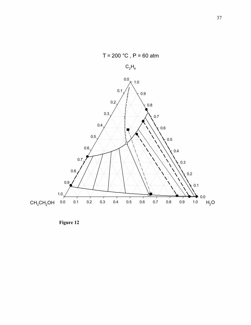
The upper and lower solid curved lines correspond to the dew-point and bubble-point loci of the
non-reacting ternary system, respectively. Several tie lines are drawn in each diagram to show the
coexisting phases at VLE equilibrium. The dew-point and bubble-point lines as well as the
corresponding solid tie lines were calculated by means of the PRSV2-WS-UNIQUAC
thermodynamic model as described in detail in the first of our previous works [1]. The dashed tie
lines correspond to the molecular simulation results. The filled circles in Figs. 9-14 correspond to
simulation results for the coexisting phases of the non-reacting system. The dotted line in the
single vapor-phase region of each diagram corresponds to the compositions of the ternary system
in vapor-phase chemical equilibrium, as calculated from the thermodynamic model, so that the
intersection point of that dotted line with the dew-point line of the non-reacting system
corresponds to the vapor phase at the combined ChVLE from the thermodynamic model. In each
diagram, the two empty squares correspond to the compositions of the two phases at the
combined ChVLE calculated from the thermodynamic model, whereas the two filled squares
correspond to the compositions of the two phases at the combined ChVLE computed from
molecular simulation.
For most of the pressures listed above, simulation predictions for the composition of the liquid
phase at the combined ChVLE (shown by the lower filled squares), turn out to be relatively close
15
to the corresponding predictions from the thermodynamic model (shown by the lower empty
squares); however, at 100 and 130 atm, the deviations between the two sets of predictions
become significant. In contrast, for most of the pressure values, simulation predictions for the
composition of the vapor phase (shown by the upper filled squares) exhibit significant deviations
with respect to the corresponding predictions from the thermodynamic model (shown by the
upper empty squares). Both sets of predictions are in relatively close agreement only at 40, 50,
and 70 atm.
In Section 3.1, from the predictions that we had previously made by means of the thermodynamic
model [1], we tested the validity of the computed values for the vapor-phase chemical
equilibrium compositions (shown in Figs. 1-4) and conversions of ethylene to ethanol (shown in
Figs. 5-8), arriving at the conclusion that at some conditions of ethylene to water feed mole ratio,
the results shown in Figs. 1-8 would be hypothetical because, in accordance with the
thermodynamic model, at those conditions, the reaction would actually occur either in a single
liquid phase or in a two-phase system. This conclusion turns out to be validated by the fact that
the portion of the vapor-phase chemical equilibrium locus that contains the points corresponding
to those conditions (see Figs. 1-4) indeed happens to fall inside the two-phase envelope (see Figs.
9-12).
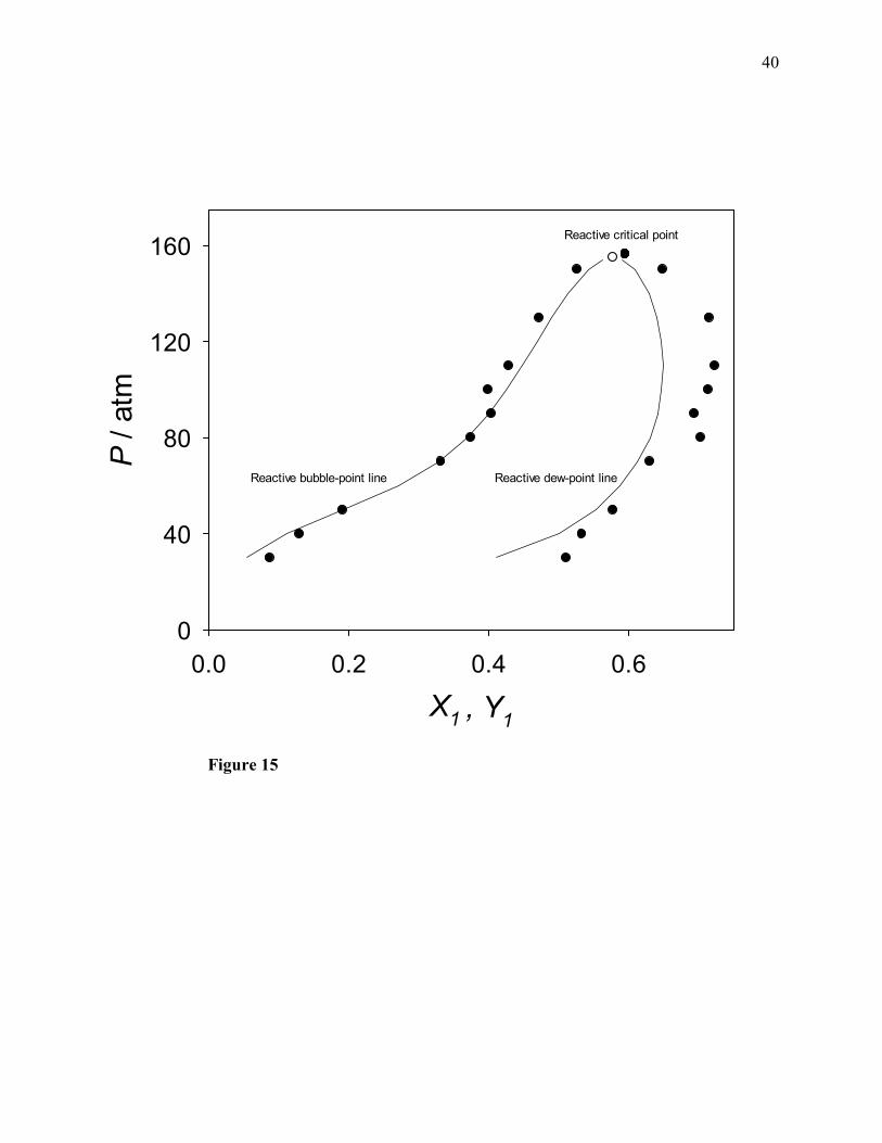
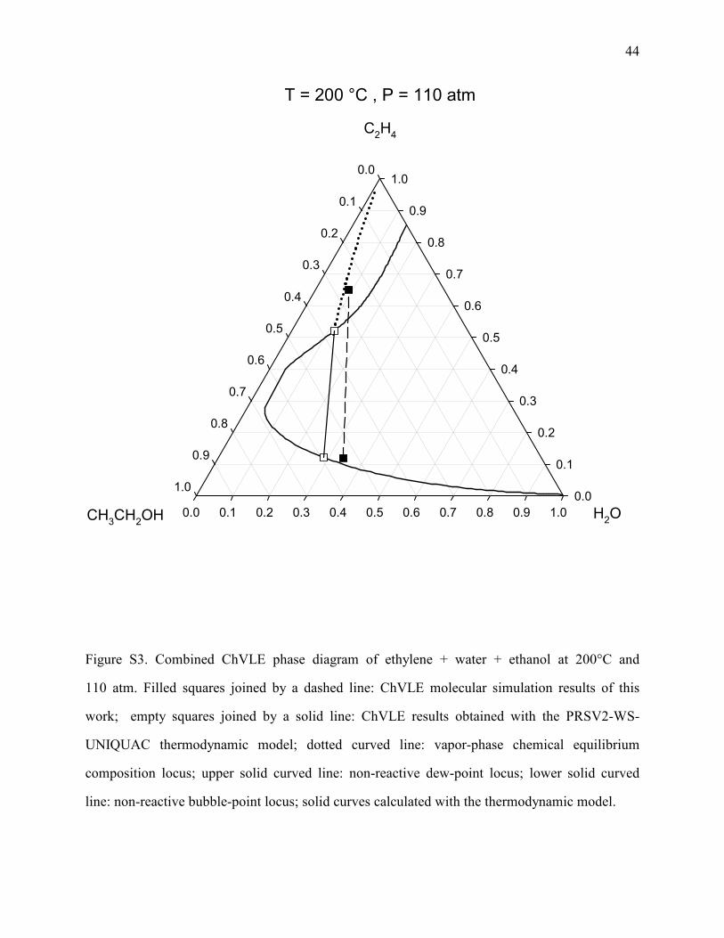
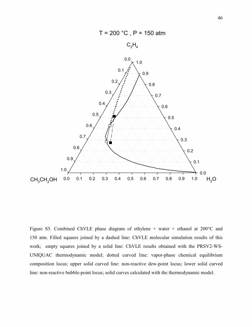
From Figs. 9-14 and S1-S5, it follows that the two phases at the combined ChVLE get richer in
ethanol and also their compositions get closer as the pressure increases from 30 to 150 atm. By
following the formulation given by Ung and Doherty [46], it is possible to gather the combined
ChVLE information given in Figs. 9-14 and S1-S5 in a single reactive phase diagram (valid at
200°C) if ethanol (3) is chosen as the reference component and transformed composition
variables are defined for ethylene (1) and water (2), as follows:
3
311
1 x
xxX
+
+= ,
3
322
1 x
xxX
+
+= (10-a)
16
3
311
1 y
yyY
+
+= ,
3
322
1 y
yyY
+
+= (10-b)
Each pair of transformed variables sum to unity; therefore, they are not independent and only one
variable of each pair is needed to plot the reactive phase diagram. From the results represented by
the empty and filled squares in Figs. 9-14 and S1-S5, the reactive phase diagram of pressure
versus transformed liquid and vapor-phase ethylene compositions ( 11,YXP − diagram) at 200°C
was plotted and is shown in Fig. 15, where the filled circles correspond to molecular simulation
results and the solid lines correspond to the results obtained by means of the thermodynamic
model, which were reported in the first of our previous works [1]. The solid line and filled circles
at the left side of the diagram correspond to the reactive bubble-point line, and the solid line and
filled circles at the right side of the diagram correspond to the reactive dew-point line. The solid
lines intersect at the point marked by the empty circle, at a pressure of 155 atm. As discussed in
our previous work [1], since the 11,YXP − plot is touched by a horizontal tangent line at that
intersection point, such a point can be regarded as a reactive critical point.
In contrast to the thermodynamic model, molecular simulation predicts a wider reactive phase
diagram (due to a reactive dew-point line much richer in ethylene). However, these two
independent approaches are in very good agreement with regard to the predicted bubble-point
line of the reactive phase diagram. Lines (not shown) passing through the upper simulation data
points intersect at a point (indicated by the topmost filled circle) which turns out to be very close
to the point marked by the empty circle. Therefore, molecular simulation agrees with the
thermodynamic model with regard to the approximate location of the reactive critical point of the
ternary system ethylene + water + ethanol.
4. Conclusions
Reaction-ensemble (RxMC) molecular simulation predictions for the vapor-phase chemical
equilibrium composition of the ternary system and the equilibrium conversion of ethylene to
ethanol (at a temperature of 200°C and pressures of 30, 40, 50, and 60 atm) are in good
17
agreement with predictions made by use of a thermodynamic model that combines the Peng-
Robinson-Stryjek-Vera equation of state, the Wong-Sandler mixing rules, and the UNIQUAC
activity coefficient model [1].
The reactive Gibbs-ensemble (RxGEMC) molecular simulation predictions for the bubble-point
line of the reactive phase diagram and the approximate location of the reactive critical point are
in very good agreement with the predictions made by means of the thermodynamic model.
However, due to a reactive dew-point line much richer in ethylene, molecular simulation predicts
a wider reactive phase diagram.
Nomenclature
C number of species in the reacting system
Bk Boltzmann constant
eqK chemical equilibrium constant
N total number of molecules
iN initial number of molecules of component i for a reaction step
P pressure
rxP probability of acceptance of a reaction step
0P standard-state pressure
T absolute temperature
U configurational energy
V volume of the simulation box
ix liquid-phase mole fraction of component i
iX transformed liquid-phase mole fraction of component i
iy vapor-phase mole fraction of component i
iY transformed vapor-phase mole fraction of component i
Greek symbols

18
χ correction factor for the Lorentz-Berthelot combining rule
iν stoichiometric coefficient of component i
ν stoichiometric coefficient of the reaction
ζ reaction direction index
Subscripts
Coul Coulombic
LJ Lennard-Jones
t total
Superscripts
(b) in the backward direction
(c) by creation
(d) by deletion
(f) in the forward direction
real real-space contribution
recip reciprocal-space contribution
self self-interaction contribution
Acknowledgement
Financial support from the Colombian Administrative Department of Science, Innovation and
Technology (COLCIENCIAS), through a research assistanship for doctoral students, and
additional financial assistance from the Thermodynamics and Energy Technology Chair of the
University of Paderborn in Germany during a doctoral-student research internship spent from
October 2013 to July 2014, are gratefully acknowledged by one of the authors (Y.M. Muñoz-
Muñoz).

19
References
[1] M. Llano-Restrepo, Y.M. Muñoz-Muñoz, Fluid Phase Equilibr. 307 (2011) 45-57.
[2] Y.M. Muñoz-Muñoz, M. Llano-Restrepo, Fluid Phase Equilibr. 394 (2015) 1-11.
[3] S.L. Weitz, J.J. Potoff, Fluid Phase Equilibr. 234 (2005) 144-150.
[4] Y.-L. Huang, T. Merker, M. Heilig, H. Hasse, J. Vrabec, Ind. Eng. Chem. Res. 51 (2012) 7428-7440.
[5] T. Schnabel, J. Vrabec, H. Hasse, Fluid Phase Equilibr. 233 (2005) 134-143.
[6] J. Smukala, R. Span, W. Wagner, J. Phys. Chem. Ref. Data 29 (2000) 1053-1121.
[7] W. Wagner, A. Pruß, J. Phys. Chem. Ref. Data 31 (2002) 387-535.
[8] H.E. Dillon, S.G. Penoncello, Int. J. Thermophys. 25 (2004) 321-335.
[9] D.S. Tsiklis, E.V. Mushkina, L.I. Shenderei, Inzh. Fiz. Zh. 1 (8) (1958) 3-7.
[10] D.S. Tsiklis, A.N. Kofman, Russ. J. Phys. Chem. 35 (1961) 549-551.
[11] F. Barr-David, B.F. Dodge, J. Chem. Eng. Data 4 (1959) 107-121.
[12] D.S. Tsiklis, A.I. Kulikova, L.I. Shenderei, Khim. Promst. (5) (1960) 401-406.
[13] D.-Y. Peng, D.B. Robinson, Ind. Eng. Chem. Fundam. 15 (1976) 59-64.
[14] R. Stryjek, J.H. Vera, Can. J. Chem. Eng. 64 (1986) 323-333.
[15] D.S.H. Wong, S.I. Sandler, AIChE J. 38 (1992) 671-680.
[16] D.S. Abrams, J.M. Prausnitz, AIChE J. 21 (1975) 116-128.
[17] W.R. Smith, B. Triska, J. Chem. Phys. 100 (1994) 3019-3027.
[18] J.K. Johnson, A.Z. Panagiotopoulos, K.E. Gubbins, Mol. Phys. 81 (1994) 717-733.
[19] C.H. Turner, J.K. Brennan, M. Lísal, W.R. Smith, J.K. Johnson, K.E. Gubbins, Mol. Simul. 34
(2008) 119-146.
[20] C.H. Turner, J.K. Johnson, K.E. Gubbins, J. Chem. Phys. 114 (2001) 1851-1859.
[21] M. Lísal, J.K. Brennan, W.R. Smith, J. Chem. Phys. 124 (2006) 064712.
[22] M. Lísal, P. Cosoli, W.R. Smith, S.K. Jain, K.E. Gubbins, Fluid Phase Equilibr. 272 (2008) 18-31.
[23] C.H. Turner, K.E. Gubbins, J. Chem. Phys. 119 (2003) 6057-6067.
[24] J. Carrero-Mantilla, M. Llano-Restrepo, Fluid Phase Equilibr. 219 (2004) 181-193.
[25] X. Peng, W. Wang, S. Huang, Fluid Phase Equilibr. 231 (2005) 138-149.
[26] M. Lísal, M. Bendová, W.R. Smith, Fluid Phase Equilibr. 235 (2005) 50-57.
[27] J. Carrero-Mantilla, M. Llano-Restrepo, Fluid Phase Equilibr. 242 (2006) 189-203.
[28] M. Lísal, I. Nezbeda, W.R. Smith, J. Chem. Phys. 110 (1999) 8597-8604.
[29] M. Lísal, W.R. Smith, I. Nezbeda, AIChE J. 46 (2000) 866-875.
[30] A.Z. Panagiotopoulos, Mol. Phys. 61 (1987) 813-826.

20
[31] A.Z. Panagiotopoulos, N. Quirke, M. Stapleton, D.J. Tildesley, Mol. Phys. 63 (1988) 527-545.
[32] A.Z. Panagiotopoulos, M.R. Stapleton, Fluid Phase Equilibr. 53 (1989) 133-141.
[33] A.Z. Panagiotopoulos, Int. J. Thermophys. 10 (1989) 447-457.
[34] B. Smit, Ph. de Smedt, D. Frenkel, Mol. Phys. 68 (1989) 931-950.
[35] B. Smit, D. Frenkel, Mol. Phys. 68 (1989) 951-958.
[36] A.Z. Panagiotopoulos, Mol. Simul. 9 (1992) 1-23.
[37] A.Z. Panagiotopoulos, J. Phys. Condens. Matter 12 (2000) 25-52.
[38] M.P. Allen, D.J. Tildesley, Computer simulation of liquids, Oxford University Press, 1989.
[39] D. Frenkel, B. Smit, Understanding molecular simulation: from algorithms to applications, Second
Edition, Academic Press, 2002.
[40] M. Llano-Restrepo, Molecular modeling and Monte Carlo simulation of concentrated aqueous alkali
halide solutions at 25°C, Ph.D. Dissertation, Rice University, Houston, 1994.
[41] M. Llano-Restrepo, W.G. Chapman, J. Chem. Phys. 100 (1994) 8321-8339.
[42] D.C. Rapaport, The art of molecular dynamics simulation, Cambridge University Press, 1998.
[43] J.J. de Pablo, J.M. Prausnitz, Fluid Phase Equilibr. 53 (1989) 177-189.
[44] R.P. Fartaria, R.S. Neves, P.C. Rodrigues, F.F. Freitas, F. Silva-Fernandes, Comp. Phys. Comm. 175
(2006) 116-121.
[45] H. Flyvbjerg, H.G. Petersen, J. Chem. Phys. 91 (1989) 461-466.
[46] S. Ung, M.F. Doherty, Chem. Eng. Sci. 50 (1995) 23-48.
VITAE
Y. Mauricio Muñoz-Muñoz received his undergraduate degree (B.S) in chemical engineering
from Universidad Nacional de Colombia, at the Manizales campus, in 2007, and his doctoral
degree (in Chemical Engineering) from Universidad del Valle, Cali, Colombia, in November
2014. He is currently working as a postdoctoral researcher in the Thermodynamics and Energy
Technology Chair of Professor Jadran Vrabec at the Faculty of Mechanical Engineering of the
University of Paderborn in Germany.
Jadran Vrabec is Professor of Thermodynamics and Energy Technology at the University of
Paderborn, Germany. He received his Ph.D. degree in Mechanical Engineering from Ruhr-

21
Universität-Bochum in 1996. His main research interests are molecular modeling and simulation,
applied experimental thermodynamics, and energy technology. In 2013, he was awarded with the
International Supercomputing Award. Some of the courses he has taught are thermodynamics,
molecular thermodynamics, rational energy use, and process engineering.
Mario Llano-Restrepo is Professor of Chemical Engineering at Universidad del Valle in Cali,
Colombia. He received his Ph.D. degree (in Chemical Engineering) from Rice University in
1994. His main research interests are modeling of phase and chemical equilibria, modeling and
simulation of separation processes, and molecular simulation. In 2009, he earned a Distinguished
Professor recognition from Universidad del Valle for service and excellence in teaching since
1994. Some of the courses he has taught are chemical thermodynamics, statistical
thermodynamics, molecular simulation, chemical reaction engineering, mass transfer, separation
operations, and separation process modeling and simulation.
Figure Captions
Figure 1. Vapor-phase chemical equilibrium composition diagram of ethylene + water + ethanol
at 200°C and 30 atm. Filled circles: molecular simulation results of this work; empty circles and
solid curved line: calculated with the PRSV2-WS-UNIQUAC thermodynamic model; empty
squares: feed compositions. Dotted lines join feed (initial) and equilibrium (final) compositions.
Figure 2. Vapor-phase chemical equilibrium composition diagram of ethylene + water + ethanol
at 200°C and 40 atm. Filled circles: molecular simulation results of this work; empty circles and
solid curved line: calculated with the PRSV2-WS-UNIQUAC thermodynamic model; empty
squares: feed compositions. Dotted lines join feed (initial) and equilibrium (final) compositions.
22
Figure 3. Vapor-phase chemical equilibrium composition diagram of ethylene + water + ethanol
at 200°C and 50 atm. Filled circles: molecular simulation results of this work; empty circles and
solid curved line: calculated with the PRSV2-WS-UNIQUAC thermodynamic model; empty
squares: feed compositions. Dotted lines join feed (initial) and equilibrium (final) compositions.
Figure 4. Vapor-phase chemical equilibrium composition diagram of ethylene + water + ethanol
at 200°C and 60 atm. Filled circles: molecular simulation results of this work; empty circles and
solid curved line: calculated with the PRSV2-WS-UNIQUAC thermodynamic model; empty
squares: feed compositions. Dotted lines join feed (initial) and equilibrium (final) compositions.
Figure 5. Vapor-phase reaction equilibrium percentage conversion of ethylene to ethanol at
200°C and 30 atm as a function of the ethylene to water feed mole ratio. Filled circles: molecular
simulation results of this work; solid curved line calculated with the PRSV2-WS-UNIQUAC
thermodynamic model; empty squares: calculated by assuming ideal-gas behavior.
Figure 6. Vapor-phase reaction equilibrium percentage conversion of ethylene to ethanol at
200°C and 40 atm as a function of the ethylene to water feed mole ratio. Filled circles: molecular
simulation results of this work; solid curved line calculated with the PRSV2-WS-UNIQUAC
thermodynamic model; empty squares: calculated by assuming ideal-gas behavior.
Figure 7. Vapor-phase reaction equilibrium percentage conversion of ethylene to ethanol at
200°C and 50 atm as a function of the ethylene to water feed mole ratio. Filled circles: molecular
simulation results of this work; solid curved line calculated with the PRSV2-WS-UNIQUAC
thermodynamic model; empty squares: calculated by assuming ideal-gas behavior.
Figure 8. Vapor-phase reaction equilibrium percentage conversion of ethylene to ethanol at
200°C and 60 atm as a function of the ethylene to water feed mole ratio. Filled circles: molecular
23
simulation results of this work; solid curved line calculated with the PRSV2-WS-UNIQUAC
thermodynamic model; empty squares: calculated by assuming ideal-gas behavior.
Figure 9. Combined ChVLE phase diagram of ethylene + water + ethanol at 200°C and 30 atm.
Filled squares joined by a dashed line: ChVLE molecular simulation results of this work; empty
squares joined by a solid line: ChVLE results obtained with the PRSV2-WS-UNIQUAC
thermodynamic model; dotted curved line: vapor-phase chemical equilibrium composition locus;
upper solid curved line: non-reactive dew-point locus; lower solid curved line: non-reactive
bubble-point locus; filled circles joined by dashed lines: non-reactive VLE molecular simulation
results; solid line segments: non-reactive VLE tie lines calculated with the thermodynamic
model.
Figure 10. Combined ChVLE phase diagram of ethylene + water + ethanol at 200°C and 40 atm.
Filled squares joined by a dashed line: ChVLE molecular simulation results of this work; empty
squares joined by a solid line: ChVLE results obtained with the PRSV2-WS-UNIQUAC
thermodynamic model; dotted curved line: vapor-phase chemical equilibrium composition locus;
upper solid curved line: non-reactive dew-point locus; lower solid curved line: non-reactive
bubble-point locus; filled circles joined by dashed lines: non-reactive VLE molecular simulation
results; solid line segments: non-reactive VLE tie lines calculated with the thermodynamic
model.
Figure 11. Combined ChVLE phase diagram of ethylene + water + ethanol at 200°C and 50 atm.
Filled squares joined by a dashed line: ChVLE molecular simulation results of this work; empty
squares joined by a solid line: ChVLE results obtained with the PRSV2-WS-UNIQUAC
thermodynamic model; dotted curved line: vapor-phase chemical equilibrium composition locus;
upper solid curved line: non-reactive dew-point locus; lower solid curved line: non-reactive
bubble-point locus; filled circles joined by dashed lines: non-reactive VLE molecular simulation
24
results; solid line segments: non-reactive VLE tie lines calculated with the thermodynamic
model.
Figure 12. Combined ChVLE phase diagram of ethylene + water + ethanol at 200°C and 60 atm.
Filled squares joined by a dashed line: ChVLE molecular simulation results of this work; empty
squares joined by a solid line: ChVLE results obtained with the PRSV2-WS-UNIQUAC
thermodynamic model; dotted curved line: vapor-phase chemical equilibrium composition locus;
upper solid curved line: non-reactive dew-point locus; lower solid curved line: non-reactive
bubble-point locus; filled circles joined by dashed lines: non-reactive VLE molecular simulation
results; solid line segments: non-reactive VLE tie lines calculated with the thermodynamic
model.
Figure 13. Combined ChVLE phase diagram of ethylene + water + ethanol at 200°C and 80 atm.
Filled squares joined by a dashed line: ChVLE molecular simulation results of this work; empty
squares joined by a solid line: ChVLE results obtained with the PRSV2-WS-UNIQUAC
thermodynamic model; dotted curved line: vapor-phase chemical equilibrium composition locus;
upper solid curved line: non-reactive dew-point locus; lower solid curved line: non-reactive
bubble-point locus; filled circles joined by dashed lines: non-reactive VLE molecular simulation
results; solid line segments: non-reactive VLE tie lines calculated with the thermodynamic
model.
Figure 14. Combined ChVLE phase diagram of ethylene + water + ethanol at 200°C and 100
atm. Filled squares joined by a dashed line: ChVLE molecular simulation results of this work;
empty squares joined by a solid line: ChVLE results obtained with the PRSV2-WS-UNIQUAC
thermodynamic model; dotted curved line: vapor-phase chemical equilibrium composition locus;
upper solid curved line: non-reactive dew-point locus; lower solid curved line: non-reactive
bubble-point locus; filled circles joined by dashed lines: non-reactive VLE molecular simulation

25
results; solid line segments: non-reactive VLE tie lines calculated with the thermodynamic
model.
Figure 15. Reactive phase diagram (pressure versus transformed liquid and vapor-phase ethylene
mole fractions) for the ternary system ethylene + water + ethanol at 200°C. Filled circles:
molecular simulation results of this work; solid lines: calculated with the PRSV2-WS-
UNIQUAC thermodynamic model; empty circle: reactive critical point predicted by
thermodynamic model; topmost filled circle: reactive critical point predicted by molecular
simulation.
26
T = 200 °C , P = 30 atm
H2O
0.0 0.1 0.2 0.3 0.4 0.5 0.6 0.7 0.8 0.9 1.0
C2H4
0.0
0.1
0.2
0.3
0.4
0.5
0.6
0.7
0.8
0.9
1.0
CH3CH2OH
0.0
0.1
0.2
0.3
0.4
0.5
0.6
0.7
0.8
0.9
1.0
Figure 1

27
T = 200 °C , P = 40 atm
H2O
0.0 0.1 0.2 0.3 0.4 0.5 0.6 0.7 0.8 0.9 1.0
C2H4
0.0
0.1
0.2
0.3
0.4
0.5
0.6
0.7
0.8
0.9
1.0
CH3CH2OH
0.0
0.1
0.2
0.3
0.4
0.5
0.6
0.7
0.8
0.9
1.0
Figure 2

28
T = 200 °C , P = 50 atm
H2O
0.0 0.1 0.2 0.3 0.4 0.5 0.6 0.7 0.8 0.9 1.0
C2H4
0.0
0.1
0.2
0.3
0.4
0.5
0.6
0.7
0.8
0.9
1.0
CH3CH2OH
0.0
0.1
0.2
0.3
0.4
0.5
0.6
0.7
0.8
0.9
1.0
Figure 3
29
T = 200 °C , P = 60 atm
H2O
0.0 0.1 0.2 0.3 0.4 0.5 0.6 0.7 0.8 0.9 1.0
C2H4
0.0
0.1
0.2
0.3
0.4
0.5
0.6
0.7
0.8
0.9
1.0
CH3CH2OH
0.0
0.1
0.2
0.3
0.4
0.5
0.6
0.7
0.8
0.9
1.0
Figure 4

30
Ethylene to water feed ratio
0 2 4 6 8 10
Eth
yle
ne
con
ve
rsio
n (
%)
0
20
40
60
Figure 5
31
Ethylene to water feed ratio
0 2 4 6 8 10
Eth
yle
ne
con
ve
rsio
n (
%)
0
20
40
60
Figure 6

32
Ethylene to water feed ratio
0 2 4 6 8 10
Eth
yle
ne
con
ve
rsio
n (
%)
0
20
40
60
80
Figure 7

33
Ethylene to water feed ratio
0 2 4 6 8 10
Eth
yle
ne
con
ve
rsio
n (
%)
0
20
40
60
80
Figure 8

34
T = 200 °C , P = 30 atm
H2O0.0 0.1 0.2 0.3 0.4 0.5 0.6 0.7 0.8 0.9 1.0
C2H
4
0.0
0.1
0.2
0.3
0.4
0.5
0.6
0.7
0.8
0.9
1.0
CH3CH
2OH
0.0
0.1
0.2
0.3
0.4
0.5
0.6
0.7
0.8
0.9
1.0
Figure 9
35
T = 200 °C , P = 40 atm
H2O0.0 0.1 0.2 0.3 0.4 0.5 0.6 0.7 0.8 0.9 1.0
C2H
4
0.0
0.1
0.2
0.3
0.4
0.5
0.6
0.7
0.8
0.9
1.0
CH3CH
2OH
0.0
0.1
0.2
0.3
0.4
0.5
0.6
0.7
0.8
0.9
1.0
Figure 10
36
T = 200 °C , P = 50 atm
H2O
0.0 0.1 0.2 0.3 0.4 0.5 0.6 0.7 0.8 0.9 1.0
C2H4
0.0
0.1
0.2
0.3
0.4
0.5
0.6
0.7
0.8
0.9
1.0
CH3CH2OH
0.0
0.1
0.2
0.3
0.4
0.5
0.6
0.7
0.8
0.9
1.0
Figure 11
37
T = 200 °C , P = 60 atm
H2O0.0 0.1 0.2 0.3 0.4 0.5 0.6 0.7 0.8 0.9 1.0
C2H
4
0.0
0.1
0.2
0.3
0.4
0.5
0.6
0.7
0.8
0.9
1.0
CH3CH
2OH
0.0
0.1
0.2
0.3
0.4
0.5
0.6
0.7
0.8
0.9
1.0
Figure 12

38
T = 200 °C , P = 80 atm
H2O0.0 0.1 0.2 0.3 0.4 0.5 0.6 0.7 0.8 0.9 1.0
C2H
4
0.0
0.1
0.2
0.3
0.4
0.5
0.6
0.7
0.8
0.9
1.0
CH3CH
2OH
0.0
0.1
0.2
0.3
0.4
0.5
0.6
0.7
0.8
0.9
1.0
Figure 13

39
T = 200 °C , P = 100 atm
H2O0.0 0.1 0.2 0.3 0.4 0.5 0.6 0.7 0.8 0.9 1.0
C2H
4
0.0
0.1
0.2
0.3
0.4
0.5
0.6
0.7
0.8
0.9
1.0
CH3CH
2OH
0.0
0.1
0.2
0.3
0.4
0.5
0.6
0.7
0.8
0.9
1.0
Figure 14
40
X1 , Y1
0.0 0.2 0.4 0.6
P /
atm
0
40
80
120
160
Reactive bubble-point line Reactive dew-point line
Reactive critical point
Figure 15
41
Supplementary Data for
Vapor-phase chemical equilibrium and
combined chemical and vapor-liquid equilibrium
for the ternary system ethylene + water + ethanol
from reaction-ensemble and reactive Gibbs-ensemble
molecular simulations
Y. Mauricio Muñoz-Muñoz a,b, Jadran Vrabecb, Mario Llano-Restrepo a*
a School of Chemical Engineering, Universidad del Valle,
Ciudad Universitaria Melendez, Building 336,
Apartado 25360, Cali, Colombia
b Thermodynamics and Energy Technology,
University of Paderborn, 33098 Paderborn, Germany
* Corresponding author. Tel: + 57-2-3312935; fax: + 57-2-3392335
E-mail address: [email protected] (M. Llano-Restrepo)

42
T = 200 °C , P = 70 atm
H2O0.0 0.1 0.2 0.3 0.4 0.5 0.6 0.7 0.8 0.9 1.0
C2H
4
0.0
0.1
0.2
0.3
0.4
0.5
0.6
0.7
0.8
0.9
1.0
CH3CH
2OH
0.0
0.1
0.2
0.3
0.4
0.5
0.6
0.7
0.8
0.9
1.0
Figure S1. Combined ChVLE phase diagram of ethylene + water + ethanol at 200°C and 70 atm.
Filled squares joined by a dashed line: ChVLE molecular simulation results of this work; empty
squares joined by a solid line: ChVLE results obtained with the PRSV2-WS-UNIQUAC
thermodynamic model; dotted curved line: vapor-phase chemical equilibrium composition locus;
upper solid curved line: non-reactive dew-point locus; lower solid curved line: non-reactive
bubble-point locus; solid curves calculated with the thermodynamic model.

43
T = 200 °C , P = 90 atm
H2O0.0 0.1 0.2 0.3 0.4 0.5 0.6 0.7 0.8 0.9 1.0
C2H
4
0.0
0.1
0.2
0.3
0.4
0.5
0.6
0.7
0.8
0.9
1.0
CH3CH
2OH
0.0
0.1
0.2
0.3
0.4
0.5
0.6
0.7
0.8
0.9
1.0
Figure S2. Combined ChVLE phase diagram of ethylene + water + ethanol at 200°C and 90 atm.
Filled squares joined by a dashed line: ChVLE molecular simulation results of this work; empty
squares joined by a solid line: ChVLE results obtained with the PRSV2-WS-UNIQUAC
thermodynamic model; dotted curved line: vapor-phase chemical equilibrium composition locus;
upper solid curved line: non-reactive dew-point locus; lower solid curved line: non-reactive
bubble-point locus; solid curves calculated with the thermodynamic model.
44
T = 200 °C , P = 110 atm
H2O0.0 0.1 0.2 0.3 0.4 0.5 0.6 0.7 0.8 0.9 1.0
C2H
4
0.0
0.1
0.2
0.3
0.4
0.5
0.6
0.7
0.8
0.9
1.0
CH3CH
2OH
0.0
0.1
0.2
0.3
0.4
0.5
0.6
0.7
0.8
0.9
1.0
Figure S3. Combined ChVLE phase diagram of ethylene + water + ethanol at 200°C and
110 atm. Filled squares joined by a dashed line: ChVLE molecular simulation results of this
work; empty squares joined by a solid line: ChVLE results obtained with the PRSV2-WS-
UNIQUAC thermodynamic model; dotted curved line: vapor-phase chemical equilibrium
composition locus; upper solid curved line: non-reactive dew-point locus; lower solid curved
line: non-reactive bubble-point locus; solid curves calculated with the thermodynamic model.

45
T = 200 °C , P = 130 atm
H2O0.0 0.1 0.2 0.3 0.4 0.5 0.6 0.7 0.8 0.9 1.0
C2H
4
0.0
0.1
0.2
0.3
0.4
0.5
0.6
0.7
0.8
0.9
1.0
CH3CH
2OH
0.0
0.1
0.2
0.3
0.4
0.5
0.6
0.7
0.8
0.9
1.0
Figure S4. Combined ChVLE phase diagram of ethylene + water + ethanol at 200°C and
130 atm. Filled squares joined by a dashed line: ChVLE molecular simulation results of this
work; empty squares joined by a solid line: ChVLE results obtained with the PRSV2-WS-
UNIQUAC thermodynamic model; dotted curved line: vapor-phase chemical equilibrium
composition locus; upper solid curved line: non-reactive dew-point locus; lower solid curved
line: non-reactive bubble-point locus; solid curves calculated with the thermodynamic model.
46
T = 200 °C , P = 150 atm
H2O0.0 0.1 0.2 0.3 0.4 0.5 0.6 0.7 0.8 0.9 1.0
C2H
4
0.0
0.1
0.2
0.3
0.4
0.5
0.6
0.7
0.8
0.9
1.0
CH3CH
2OH
0.0
0.1
0.2
0.3
0.4
0.5
0.6
0.7
0.8
0.9
1.0
Figure S5. Combined ChVLE phase diagram of ethylene + water + ethanol at 200°C and
150 atm. Filled squares joined by a dashed line: ChVLE molecular simulation results of this
work; empty squares joined by a solid line: ChVLE results obtained with the PRSV2-WS-
UNIQUAC thermodynamic model; dotted curved line: vapor-phase chemical equilibrium
composition locus; upper solid curved line: non-reactive dew-point locus; lower solid curved
line: non-reactive bubble-point locus; solid curves calculated with the thermodynamic model.