■ The Vanguard Capital Markets Model® (VCMM) is a proprietary financial simulation engine that is designed to help clients make effective asset allocation decisions. The VCMM comprises two main elements: (1) a global, dynamic model that simulates return distributions for a wide array of asset classes; and (2) asset allocation tools to assist in the construction of portfolio solutions.

■ Key features of the asset-return simulation model in the VCMM include a probabilistic (distributional) framework, forward-looking return assumptions, a dependence on current market conditions, and the use of non-normal distributions.

■ The simulated output, consisting of distributions of asset returns, volatilities, and correlations, is used in multiple portfolio and research applications for personal and institutional investors globally.

Joseph Davis, Ph.D.; Roger Aliaga-Díaz, Ph.D.; Harshdeep Ahluwalia; Frank Polanco, Ph.D., CFA; Christos Tasopoulos

The buck stops here: Vanguard money market funds

Vanguard Research November 2014

Vanguard Global Capital Markets Model

The Vanguard Capital Markets Model is a proprietary model of the global capital markets, developed by Vanguard’s Investment Strategy Group. The statistical model simulates forward-looking asset-return distributions for a broad array of asset classes and risk factors.

The goal of the VCMM is to evaluate client portfolios and to provide investors with a powerful distributional framework to examine the quantitative trade-offs among alternative portfolio allocations. This examination of multi-asset-class portfolios is based on initial market conditions as well as risk-and-return assumptions, which are dynamic and forward-looking, and include distributional tail events. The VCMM forms the basis for Vanguard’s global capital markets outlook.

This paper examines the main characteristics of the asset-return simulation model within the VCMM. First, we present the logic and design of the VCMM—specifically, we describe its core statistical engine, simulation generator, and framework. Second, we discuss the global capital markets equilibrium assumptions and other important features of the model, including its incorporation of advanced financial simulations. We conclude by discussing the value of the VCMM’s forward-looking return projections in diverse investment applications while also acknowledging caveats in the model’s use.

Need for model-based financial simulations

Portfolio construction continues to evolve toward top-down strategies for global asset allocation, as opposed to bottom-up techniques of security selection. This evolution means that investors need more sophisticated financial simulation models to evaluate the range of potential portfolio outcomes. Although individual security selection requires deeper company-level and industry-sector research, asset allocation relies on a broader analysis of capital markets. Such analysis includes a thorough understanding of the key economic and financial drivers of asset returns. Quantitative models of capital markets play a prominent role in creating internally consistent asset-return expectations. These expectations include realistic projections for volatility and diversification across various asset classes.

Earlier financial simulation techniques, such as time-pathing and basic Monte Carlo simulations, relied on historical asset returns and assumed that return distributions could be directly extrapolated from history. However, as we explain in more detail in this paper, there are limitations in using these techniques under such assumptions of extrapolation (see also Davis, 2006).

Model-based simulations such as the VCMM use historical data of economic and financial drivers of asset returns to estimate and calibrate a model of the global capital markets (see Figure 1). The model is then used

2

Vanguard’s approach to forecasting and notes on risk

To treat the future with the deference it deserves, Vanguard believes that market forecasts are best viewed in a probabilistic framework. This publication’s primary objectives are to describe the projected long-term return distributions that contribute to strategic asset allocation decisions, and to present the rationale for the ranges and probabilities of potential outcomes.

IMPORTANT: The projections or other information generated by the VCMM regarding the likelihood of various investment outcomes are hypothetical in nature, do not reflect actual investment results, and are not guarantees of future results. Distribution of return outcomes from the VCMM are derived from 10,000 simulations for each modeled asset class. Simulations as of March 31, 2014. Results from the model may vary with each use and over time. For more information, please see the appendix.

All investing is subject to risk, including the possible loss of the money you invest. Past performance is no guarantee of future returns. Investments in bond funds are subject to interest rate, credit, and inflation risk. Foreign investing involves additional risks, including currency fluctuations and political uncertainty. Diversification does not ensure a profit or protect against a loss in a declining market. There is no guarantee that any particular asset allocation or mix of funds will meet your investment objectives or provide you with a given level of income. The performance of an index is not an exact representation of any particular investment, as you cannot invest directly in an index.

Equities of companies in emerging markets are generally more risky than equities of companies in developed countries. U.S. government backing of Treasury or agency securities applies only to the underlying securities and does not prevent price fluctuations. Investments that concentrate on a relatively narrow market sector face the risk of higher price volatility.

Neither diversification nor asset allocation can serve as a guarantee against a loss of principal in a market decline.

1 The VCMM can be technically characterized as a factor-augmented vector autoregression (FAVAR) model (see, for example, He and Medeiros [2011] or Bernanke, Boivin, and Eliasz [2004] and references cited in each). However, the actual implementation of the VCMM supplements the basic statistical framework with various proprietary, long-run restrictions and different distributional assumptions.

as the data-generating process, in combination with Monte-Carlo methods to derive both expectations and distributional properties of asset returns. This approach captures important aspects of asset-return simulations such as:

• Incorporating current market conditions and the serial correlation of asset returns.

• Forming forward-looking return forecasts, based on model-calibrated capital markets equilibrium.

• Producing non-normal distributions to better account for fat-tails and extreme-tail events.

• Accounting for market-consensus expectations derived from current-market asset prices.

Other methodologies that do not rely on a capital markets model may not capture all of these aspects.

The VCMM framework

The VCMM is built on the principle that potential returns from an asset class are compensation for bearing the systematic risk (or beta) of that asset class. The VCMM uses both historical macroeconomic and financial market data to dynamically model the return behavior of these asset classes. Some of these variables include, for example, yield curves, inflation, and leading economic indicators. Using large datasets of quarterly frequency starting from as early as 1960, the VCMM estimates a dynamic statistical relationship between risk factors and asset returns.1 Based on these calculations, the model generates simulations using regression-based Monte- Carlo techniques to project these relationships into the future.

3

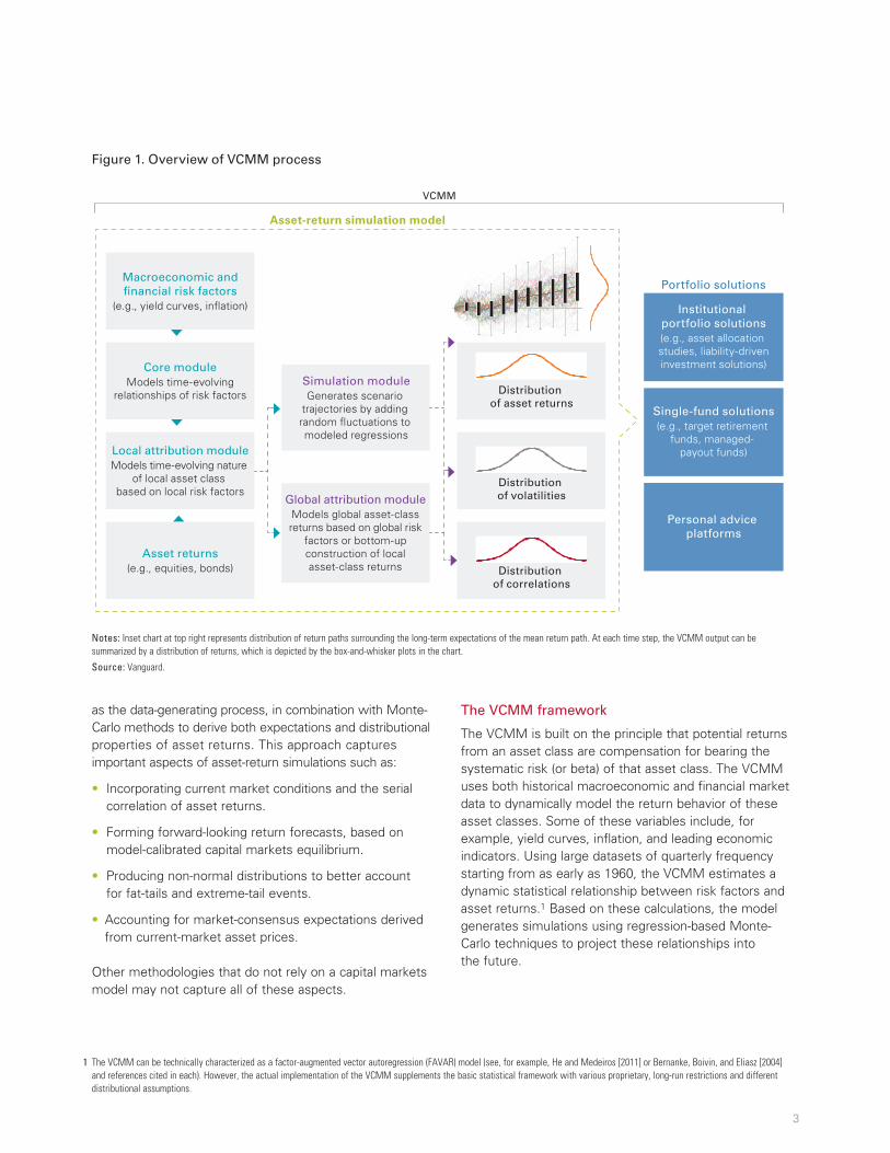
Figure 1. Overview of VCMM process

VCMM

Distribution of correlations

Distribution of volatilities

Distribution of asset returns

Core moduleModels time-evolving

relationships of risk factors

Local attribution moduleModels time-evolving nature

of local asset class based on local risk factors

Asset returns(e.g., equities, bonds)

Macroeconomic and�nancial risk factors

(e.g., yield curves, in�ation)

Global attribution moduleModels global asset-classreturns based on global risk

factors or bottom-upconstruction of localasset-class returns

Simulation moduleGenerates scenario

trajectories by adding random �uctuations to modeled regressions

Asset-return simulation model

Institutional portfolio solutions(e.g., asset allocation studies, liability-driveninvestment solutions)

Single-fund solutions(e.g., target retirement

funds, managed- payout funds)

Personal advice platforms

Portfolio solutions

Notes: Inset chart at top right represents distribution of return paths surrounding the long-term expectations of the mean return path. At each time step, the VCMM output can be summarized by a distribution of returns, which is depicted by the box-and-whisker plots in the chart.

Source: Vanguard.

2 Namely, Monte Carlo methods applied to the residuals of the core VAR and attribution regressions.

Asset-return simulation model

The asset-return simulation model in the VCMM has four main modules:

1. The core module, a dynamic model of various macroeconomic and financial risk factors or drivers.

2. The local attribution module, which contempo-raneously links local asset-class returns with regional risk factors.

3. The global attribution module, which forecasts global asset-class returns based on a combination of regional returns or global core risk factors, and also incorporates local currencies.

4. The simulation module, which combines these modeled relationships using regression-based Monte Carlo methods to generate a range of potential future returns.

Figure 2 displays the interactions of these VCMM modules and includes examples of factors and asset classes modeled in the core, attribution, and global modules. Each module is also described in more detail next.

Core module. The VCMM core module is a dynamic statistical model of regional macroeconomic and financial risk factors and determines relationships between these macroeconomic and financial risk factors. Vector autoregression (VAR) techniques, which are statistical models that can capture the time-evolving behavior of interrelated time series, are used to model the core factors. A VAR technique models each region’s core factors; that is, there are as many VARs as there are regions modeled. As shown in Figure 2, each region’s VAR model is connected to the others through the correlation of residuals (a correlation matrix of the VAR-estimated residuals). This framework of residual correlation enables shocks in one region to be appropriately transmitted to another region during the simulations. The module can then be used to project the estimated relationships into the future over any time horizon.

The VAR technique models three main categories of risk factors in the core module:

1. Local equity factors, which are the core drivers of asset prices that are strongly linked to performance of domestic equity markets.

2. Local fixed income factors, including yield curves for government bonds (considered leading indicators). These modeled yield curves describe the entire term structure (ranging in duration from one quarter to 30 years) and are based on the dynamic relationship between economic activity and inflationary expectations.

3. Local economic factors, which include inflation and proprietary leading indicators of economic activity and fluctuations in the local business cycle.

A key strength of the VCMM is the regression- based framework used to simultaneously model the core factors, thus capturing dynamically important interrelationships.

Local attribution module. Regional asset-class returns are modeled in the local attribution module, using regressions based on the core module’s regional risk factors. The module’s main function is to map the returns of those asset classes to contemporaneous changes in the appropriate core factors using regression techniques.

Global attribution module. The global attribution module forecasts global asset-class returns based on a combination of regional returns or core risk factors. Asset-return benchmarks, such as global bonds or global equity indexes, are constructed in this module, which also includes foreign exchange markets, allowing the translation of asset returns from local currency into another foreign currency.

Simulation module. This module generates scenarios (that is, different potential futures) for all risk factors and asset classes modeled in both the core and attribution modules. These scenarios, which are generated using a regression-based Monte Carlo approach,2 result in a distribution of return paths instead of single-point forecasts.

4

All simulated paths of future returns start from the same current economic and financial market conditions (that is, initial conditions). The regression-based simulation technique allows for a rich dynamic of asset-class returns as they eventually revert from initial conditions to target equilibrium levels over the long term, that is, to a steady-state condition. These steady-state targets are informed by historical estimates of long-term economic and financial factors, but are tempered using qualitative judgment. As we discuss later in this paper, for example, qualitative judgment might set target inflation lower than historical inflation averages because of structural changes in financial markets.

The model’s simulation outputs can also be summarized in reports containing key statistical characteristics of the vast amount of simulated data. An array of summary statistics, including means, medians, and standard deviations, are tabulated for the different asset-class returns at various forecast horizons. In addition, once these potential returns are generated, portfolio analyses can be run using the underlying simulated paths. A later section of this paper examines the various applications of the VCMM forecasts.

5

Figure 2. Four modules of asset-return simulation model in VCMM

U.S. core factors: (e.g., equity, yield

curve, and economic risk factors)

Australia core factors

U.K. core factors

Japan core factors

German core factors

Other core factors

U.S. asset-class return attribution:

(e.g., equities, government bonds, cash, TIPS, credit bonds, REITs, etc.)

Australia asset-class return attribution

German asset-class return attribution

Japan asset-class return attribution

U.K. asset-class return attribution

Other regional asset-return attribution

Global asset-class return attribution in various local currencies: (e.g., bottom-up construction of global equity and global bond asset classes)

Currency model (relative purchasing power parity):

USD/AUD

USD/GBP

USD/JPY

USD/EUR

Local market initial conditions and Monte Carlo methods (Output: returns, volatility, and correlations)

Currency overlay:

— Returns, volatility, and correlations for all currencies

— Conversion of asset returns to any currency

Eurozone core factors

Eurozone asset-class return attribution

Residual correlations Residual correlations

Core module (dynamic factors)

Attribution module(local asset classes)

Global attribution module(global asset-class attribution and currency model)

Simulation module

Note: Regions modeled by the VCMM—normally modeled as market-capitalization weighted—were chosen to capture the vast majority of capital markets and to help answer portfolio questions from Vanguard clients.

Source: Vanguard.

3 Mean-reversion is the key feature of stationary series such as growth rates and asset returns (discussed later).

Global capital markets equilibrium

The long-run equilibrium embedded in the VCMM plays a crucial role in formulating long-term asset-return expectations that are truly forward-looking, as opposed to being confined by history. Moreover, where appropriate, the VCMM is independent of any choice of historical data sample. Essentially, the VCMM equilibrium represents Vanguard’s best thinking on how global capital markets can be expected to operate over the very long term under normal conditions (see Figure 3). Each long-run equilibrium target is independent of the actual model and is qualitative in nature.

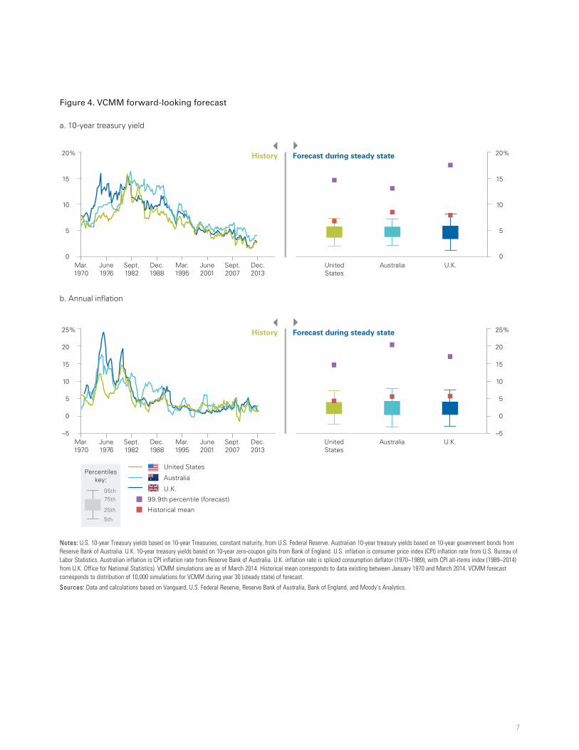
Left to their own devices, dynamic statistical models always display mean-reversion to historical average returns.3 However, sample means estimated from limited historical datasets may lead to biased projections of future asset-return expectations. The VCMM replaces raw historical averages with alternative forward-looking capital markets equilibrium assumptions, so that the simulated variables “revert” toward this equilibrium instead of to their historical average values. As Figure 4 shows, simply extrapolating the historical averages, which are highly sample-dependent, might result in misleading returns expectations that could result in inadequate portfolio allocations.

6

Figure 3. Global capital markets equilibrium assumptions: Conceptual framework

Global equities return: Short rate + Equity risk premiumGlobal bonds return: Short rate + Term premium + Credit-risk premium + In�ation-risk premiumCash return: Real (short) interest rate + In�ation target

Exp

ecte

d re

turn

Total risk = Systematic risk + Diversi�able risk

Cash

Global equitiesSectors, styles

Individual countries

Currency exposures

Regions/United States

Distribution of expected return

Global bonds

Long-term bonds

Individual countries

TIPS

Default risk premiumIn�ation-risk premium

Credit and high yield

Regions/United States

Individual country, sector, and style exposures

Notes: This figure’s view is ex ante (before the event), and expected returns are arithmetic returns. The chart is cast in local currency returns (equal to hedged returns in equilibrium). Equilibrium unhedged returns are expected to have same median as hedged returns, but with more volatility.

Source: Vanguard.

7

Figure 4. VCMM forward-looking forecast

a. 10-year treasury yield

0

5

10

15

20%

Mar.1970

June1976

Sept.1982

Dec.1988

Mar.1995

June2001

Sept.2007

Dec.2013

0

5

10

15

20%

Australia U.K.UnitedStates

History Forecast during steady state

b. Annual inflation

–5

5

0

10

15

20

25%

Mar.1970

June1976

Sept.1982

Dec.1988

Mar.1995

June2001

Sept.2007

Dec.2013

–5

5

0

10

15

20

25%

UnitedStates

Australia U.K.

United States

Australia

U.K.

99.9th percentile (forecast)

Historical mean5th

95th 75th

25th

Percentileskey:

History Forecast during steady state

Notes: U.S. 10-year Treasury yields based on 10-year Treasuries, constant maturity, from U.S. Federal Reserve. Australian 10-year treasury yields based on 10-year government bonds from Reserve Bank of Australia. U.K. 10-year treasury yields based on 10-year zero-coupon gilts from Bank of England. U.S. inflation is consumer price index (CPI) inflation rate from U.S. Bureau of Labor Statistics. Australian inflation is CPI inflation rate from Reserve Bank of Australia. U.K. inflation rate is spliced consumption deflator (1970–1989), with CPI all-items index (1989–2014) from U.K. Office for National Statistics). VCMM simulations are as of March 2014. Historical mean corresponds to data existing between January 1970 and March 2014. VCMM forecast corresponds to distribution of 10,000 simulations for VCMM during year 30 (steady state) of forecast.

Sources: Data and calculations based on Vanguard, U.S. Federal Reserve, Reserve Bank of Australia, Bank of England, and Moody’s Analytics.

Such equilibrium assumptions do not overlook history, since historical data provide a good starting point for them. In the VCMM, the calibration of equilibrium conditions for long-term risk factors combines historical data relationships with a theoretical framework as represented in Figure 3. Consider, for example, equity-return volatility: Ex ante (that is, before the event), we would expect higher volatility from an individual country compared with the global equity index, which is market-cap-weighted. Therefore in Figure 5, a country’s equity risk plots to the right of the global equity risk.

Other important features of VCMM

For any model that is global in nature, an appropriate treatment of foreign exchange markets is critical to the internal consistency of the model. In the VCMM, currencies are modeled as an overlay to asset returns, not as a risk factor. That is, asset-return projections do not depend statistically on currency factors, they are just denominated in a given currency. By having simulations of various foreign exchange markets, local currency asset returns can be easily converted across different foreign currencies. This conversion is critical for the bottom-up construction of global asset-return benchmarks, such as global equity or global bond indexes.

8

Figure 5. Equity risk and return during equilibrium

Risk (volatility)

0% 252015 30 35

10

8

6

4

2

0

12%

Global equities (hedged in USD)

Global ex-U.S. equities (hedged in USD)

U.S. equities

Eurozone equities (hedged in USD)

U.K. equities (hedged in USD)

Japan equities (hedged in USD)

Australian equities (hedged in USD)

Ten

-yea

r an

nu

aliz

ed

retu

rn in

eq

uili

bri

um

Risk–return convergence

Notes: Risk–return calculations correspond to median values of 10,000 simulations from VCMM conforming to ten years after steady state (equilibrium) is reached. Median returns are geometric returns, and regions with higher volatility have a lower median geometric return. See appendix section titled “Indexes used in our calculations,” for details of indexes. VCMM simulations are as of March 2014.

Source: Vanguard.

4 The model simulates currency returns relative to the USD. Other currency return pairs can be derived simply by taking the ratio of USD-based currency returns.

5 In other words, uncovered interest rate parity (UIP).

Figure 6 displays an example of the simulated projections for the U.S. dollar/Australian dollar (USD/AUD) market.4

The median VCMM forecast (depicted in the figure by the blue line) matches the exchange rate implied by the interest rate differential5 between the two countries at various maturities, as depicted by the blue squares in the figure, for short and intermediate periods. The exchange rate implied by the interest rate differential can be thought of as the market expectation for future spot exchange rates. The expectations built into the foreign exchange forecast are risk neutral in nature and, on average, there

is no compensation for the added level of uncertainty in equilibrium. Hence, the figure shows that the VCMM currency forecast does not impose any views other than what is already priced in by the markets. If the market believes that a currency is initially over- or undervalued, then today’s term structure of interest rates itself will indicate a subsequent correction in the currency. The 25th and 75th percentile VCMM forecasts (dashed lines) are also shown in Figure 6, along with two sample USD/AUD rate paths from the 10,000 VCMM simulations.

9

Figure 6. A currency forecast example, constructed from implied forward rates

US

D/A

UD

fo

reig

n

exch

ang

e (F

X)

rate

0

0.4

0.8

1.2

1.6

2.0

1990 1995 2000 2005 2010 2015 2020 2025 2030 2035 2040 2045

USD/AUD historyUSD/AUD forecast median25th/75th percentile boundsSample pathsUncovered interest parity (UIP) implied FX value

Projection

Notes: Forecast corresponds to distribution of 10,000 simulations from VCMM. USD per AUD Q1 1990–Q1 2014 history from Moody’s Analytics. VCMM forecast and calculated UIP implied foreign exchange values as of March 2014.

Sources: Vanguard and Moody’s Analytics.

6 The distributional parameters of the residuals are estimated as a t-distribution instead of a normal distribution. The degrees of freedom of a t-distribution determine the “fatness” of the tails. To account for cross-correlation between residuals, the covariance matrix of the residuals is estimated. Thus VCMM adopts a multivariate t-distribution fitted with varying degrees of freedom. Copula methods, along with the t-distribution parameters and the covariance matrix, are used to simulate the multivariate t-distributions.

Return forecasts for global ex-U.S. equity and global equity are constructed from the individual country or region equity-return forecasts as shown in Figure 7. As an initial output from the VCMM, return forecasts for regional equities are available in their local currencies. Combined with the currency-return forecast, these return forecasts of local equity are converted to a common currency (in this case, to the U.S. dollar). The weighted average of the country or region equity returns results in the desired return forecast for global (ex-region) equity. This bottom-up approach ensures that the equity forecasts in the VCMM are internally consistent.

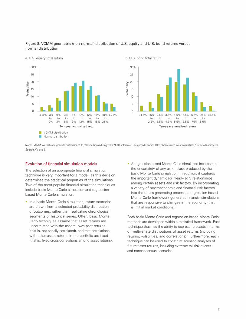
Another key feature of the model is its flexibility in terms of distributional assumptions. Asset-return distributions and distributions of other economic and financial factors often exhibit non-normal patterns. Figure 8 illustrates some of the VCMM’s non-normal distributions. The VCMM return distribution (of forecast U.S. equity and U.S. aggregate bonds) is compared in Figure 8 using

both a normal distribution and a non-normal distribution (used in the VCMM) during forecast equilibrium (years 21–30). The non-normal distribution shown has fatter tails than a normal distribution and is more representative of the financial markets.6

The estimation of residual parameters and generation of residuals is an example of the innovation used in constructing the VCMM simulations. Residuals measure the difference between predicted values from the fitted model and observed values. Often residuals are assumed to be normally distributed and independent from the residuals associated with other model variables. The VCMM allows for both heavy-tailed and correlated distributions of the residuals. Both these extensions mimic the behavior seen in financial markets, where (i) rare events occur more frequently than would be predicted by normal distributions and (ii) the magnitude of variability in different model outputs appears to be correlated.

10

Figure 7. Sample ten-year annualized return distribution in equilibrium for global ex-U.S. and global equities

Ten

-yea

r an

nu

aliz

ed r

etu

rn

–10

–5

0

5

10

15

20

25

30%

Global($)

UnitedStates

($)

Global ex-U.S.

($)

EM ($)Japan ($) EU ($)U.K. ($)AUS ($)USDEmergingmarkets

JPYJapan

EUREurozone

GBPUnited

Kingdom

AUDAustralia

=+FX

Equity forecast in local currency Equity forecast in unhedged USD

Market-cap-weighted return

5th

95th

75th

25th

Percentileskey:

Notes: Returns correspond to a distribution of 10,000 simulations from VCMM over the projected next ten years after reaching steady state (equilibrium). VCMM simulations are as of March 2014. See appendix section titled “Indexes used in our calculations,” for details of indexes.

Sources: Vanguard and Thomson Reuters Datastream.

Evolution of financial simulation models

The selection of an appropriate financial simulation technique is very important for a model, as this decision determines the statistical properties of the simulations. Two of the most popular financial simulation techniques include basic Monte Carlo simulation and regression-based Monte Carlo simulation.

• In a basic Monte Carlo simulation, return scenarios are drawn from a selected probability distribution of outcomes, rather than replicating chronological segments of historical series. Often, basic Monte Carlo techniques assume that asset returns are uncorrelated with the assets’ own past returns (that is, not serially correlated), and that correlations with other asset returns in the portfolio are fixed (that is, fixed cross-correlations among asset returns).

• A regression-based Monte Carlo simulation incorporates the uncertainty of any asset class produced by the basic Monte Carlo simulation. In addition, it captures the important dynamic (or “lead–lag”) relationships among certain assets and risk factors. By incorporating a variety of macroeconomic and financial risk factors into the return-generating process, a regression-based Monte Carlo framework generates financial simulations that are responsive to changes in the economy (that is, initial market conditions).

Both basic Monte Carlo and regression-based Monte Carlo methods are developed within a statistical framework. Each technique thus has the ability to express forecasts in terms of multivariate distributions of asset returns (including returns, volatilities, and correlations). Furthermore, each technique can be used to construct scenario analyses of future asset returns, including extreme-tail risk events and nonconsensus scenarios.

11

Figure 8. VCMM geometric (non-normal) distribution of U.S. equity and U.S. bond returns versus normal distribution

a. U.S. equity total return b. U.S. bond total return

Pro

bab

ility

Ten-year annualized return Ten-year annualized return

0

5

10

15

20

25

30%

VCMM distributionNormal distribution

<1.5% 1.5%to

2.5%

2.5%to

3.5%

3.5%to

4.5%

4.5%to

5.5%

5.5%to

6.5%

6.5%to

7.5%

7.5%to

8.5%

>8.5%<–3% –3%to 0%

0%to

3%

3%to

6%

6%to

9%

9%to

12%

12%to

15%

15% to

18%

18% to

21%

>21%

Pro

bab

ility

0

5

10

15

20

25

30%

Notes: VCMM forecast corresponds to distribution of 10,000 simulations during years 21–30 of forecast. See appendix section titled “Indexes used in our calculations,” for details of indexes.

Source: Vanguard.

7 For extreme time horizons—namely greater than 30 years—the difference in annualized returns between these methodologies becomes smaller. In particular, this difference is reduced for the interquartile range (from the 25th to 75th percentiles) as the initial conditions decay and returns converge to their targets. Thus although the regression-based Monte Carlo technique is a significant improvement over all time horizons, the traditional techniques may be adequate for financial-planning exercises over extreme time horizons.

12

Regression-based Monte Carlo simulations, however, offer an important advantage in that they can capture current market conditions and the serial correlation of asset returns. This feature shows up in asset-return forecasts that are much more sensitive to changing market conditions, such as changes in stock-valuation multiples or changing interest rates. Figure 9 illustrates two examples of the important differences between basic Monte Carlo simulations and the VCMM’s regression-based Monte Carlo simulations. The figure shows the 25th- and 75th- percentile forecasts of ten-year annualized returns.7 These out-of-sample forecasts (in U.S. dollars) are for global equities and global aggregate bond returns beginning in December 2009. For example, the December 2009 forecast is a ten-year-ahead forecast that was generated using historical data on or before December 1999.

As expected, the forecast returns generated by basic Monte Carlo techniques (the dashed lines in Figure 9) revert to the historical mean immediately. The slight temporal changes in the basic Monte Carlo out-of-sample forecasts simply reflect changes in the historical mean returns. Conversely, Figure 9 also reveals considerable sensitivity in the forecasts for the regression-based Monte Carlo approach. The greater responsiveness of return forecasts occurs because a dynamic regression-based framework accounts for the initial conditions of various persistent, slow-moving (core) factors—such as the level of interest rates or equity-market valuations. For instance, the evolution of the ten-year annualized return for global equity using the regression-based Monte-Carlo technique does not immediately revert to its long-term mean. Rather, it evolves over time, depending upon the initial conditions of financial and macroeconomic risk factors.

Figure 9. Benefits of regression-based Monte Carlo simulations on long-term return forecasts for global bonds and global equity

a. Global bonds b. Global equities

Ten

-yea

r an

nu

aliz

ed r

etu

rn

0

2

4

6

8

10

12%

Monte Carlo: 25th- and 75th-percentile boundsVCMM 25th- and 75th-percentile boundsActual

20132012201120102009

Ten

-yea

r an

nu

aliz

ed r

etu

rn

–4

4

6

8

10

12

14%

2009 2010 2011 2012 2013

2

0

–2

Notes: VCMM return forecast (ten-year-ahead and ten-year annualized returns) corresponds to distribution of 10,000 simulations in USD. For example, the ten-year-ahead forecast for December 2009 was generated using historical data on or before December 1999, and the ten-year-ahead forecast for December 2010 was generated using historical data on or before December 2000. Actual returns are authors’ calculations based on Barclays Global Aggregate Bond Index returns from Barclays Live and MSCI ACWI Index returns from Bloomberg. Also note that this figure represents historical out-of-sample forecasts of what the model could have presented if it were in its current state starting December 1999.

Sources: Vanguard, Barclays Live, and Bloomberg.

8 Equity, fixed income, and economic risk factors were all used to generate Figure 10’s analysis. However, for purposes of this paper’s discussion, only a subgroup of factors is displayed.

9 Later in the text, we discuss limitations and caveats for using VCMM forecasts.

13

Figure 9 shows that the actual ten-year annualized returns fall within the 25th- and 75th-percentile VCMM forecasts most of the time (100% of the period for global equity and more than 83% of the period for global aggregate bonds). Most important, it’s worth noting that the distribution of VCMM forecast moves in the same direction as the actual returns. The correlation between actual returns and the VCMM forecast median is 0.94 for global aggregate bonds and 0.95 for global equities. A key goal of the VCMM framework is to capture all the distributional properties of asset returns, not just point forecasts of average returns. Volatility of returns, correlations between various asset-class returns, and correlations between asset-class returns and risk factors (equity factors, yield-curve factors, and economic factors) are all important.

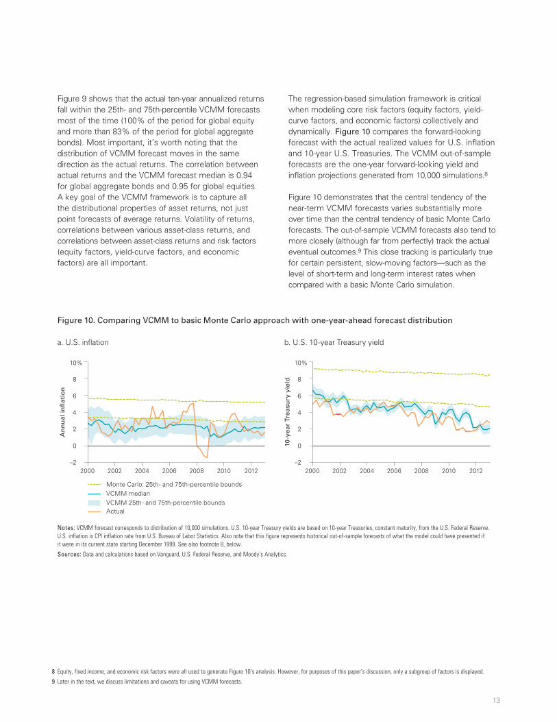
The regression-based simulation framework is critical when modeling core risk factors (equity factors, yield-curve factors, and economic factors) collectively and dynamically. Figure 10 compares the forward-looking forecast with the actual realized values for U.S. inflation and 10-year U.S. Treasuries. The VCMM out-of-sample forecasts are the one-year forward-looking yield and inflation projections generated from 10,000 simulations.8

Figure 10 demonstrates that the central tendency of the near-term VCMM forecasts varies substantially more over time than the central tendency of basic Monte Carlo forecasts. The out-of-sample VCMM forecasts also tend to more closely (although far from perfectly) track the actual eventual outcomes.9 This close tracking is particularly true for certain persistent, slow-moving factors—such as the level of short-term and long-term interest rates when compared with a basic Monte Carlo simulation.

Figure 10. Comparing VCMM to basic Monte Carlo approach with one-year-ahead forecast distribution

a. U.S. inflation b. U.S. 10-year Treasury yield

An

nu

al in

�at

ion

–2

0

2

4

6

8

10%

Monte Carlo: 25th- and 75th-percentile boundsVCMM medianVCMM 25th- and 75th-percentile boundsActual

2012201020082006200420022000

10-y

ear

Trea

sury

yie

ld

–2

0

2

4

6

8

10%

2012201020082006200420022000

Notes: VCMM forecast corresponds to distribution of 10,000 simulations. U.S. 10-year Treasury yields are based on 10-year Treasuries, constant maturity, from the U.S. Federal Reserve. U.S. inflation is CPI inflation rate from U.S. Bureau of Labor Statistics. Also note that this figure represents historical out-of-sample forecasts of what the model could have presented if it were in its current state starting December 1999. See also footnote 8, below.

Sources: Data and calculations based on Vanguard, U.S. Federal Reserve, and Moody’s Analytics.

10 See Davis et al. (2014).

14

Portfolio solutions and other uses of VCMM

The simulated output from the VCMM asset-return simulation model (consisting of distributions of asset returns, volatilities, and correlations) is used in multiple portfolio models and research applications for personal and institutional investors. Typical uses of the VCMM are:

• Long-term return expectations for Vanguard’s Economic and Market Outlook, which offers an in-depth perspective on the global markets.10

• Analyses of single-fund solutions such as life-cycle funds, college savings plans, managed-payout funds, and other diversified portfolio funds.

• Portfolio solution models to support asset allocation studies for institutional clients.

• Liability-driven investing solutions for defined benefit (DB) plans (see Stockton, 2014).

• Scenario analyses and studies of probability of meeting investment objectives for personal advice.

The VCMM is capable of performing the analyses just mentioned not only in the United States but also in other major regions such as Australia, the U.K., and Europe, among others.

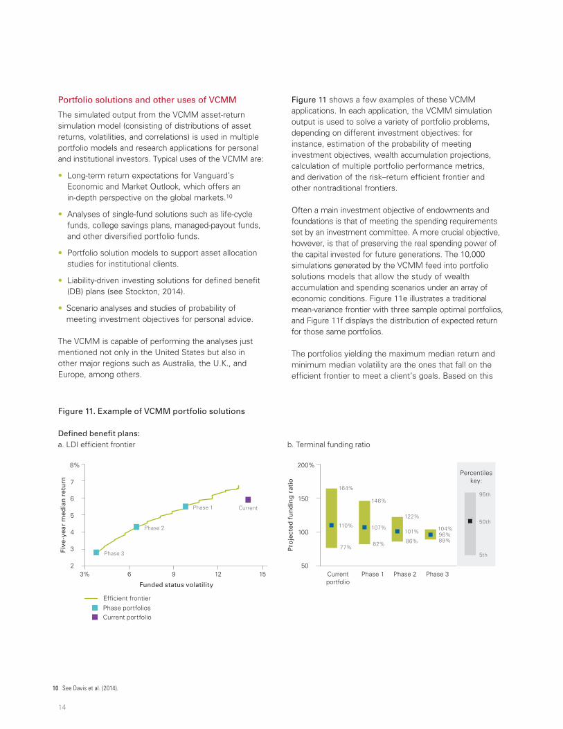
Figure 11 shows a few examples of these VCMM applications. In each application, the VCMM simulation output is used to solve a variety of portfolio problems, depending on different investment objectives: for instance, estimation of the probability of meeting investment objectives, wealth accumulation projections, calculation of multiple portfolio performance metrics, and derivation of the risk–return efficient frontier and other nontraditional frontiers.

Often a main investment objective of endowments and foundations is that of meeting the spending requirements set by an investment committee. A more crucial objective, however, is that of preserving the real spending power of the capital invested for future generations. The 10,000 simulations generated by the VCMM feed into portfolio solutions models that allow the study of wealth accumulation and spending scenarios under an array of economic conditions. Figure 11e illustrates a traditional mean-variance frontier with three sample optimal portfolios, and Figure 11f displays the distribution of expected return for those same portfolios.

The portfolios yielding the maximum median return and minimum median volatility are the ones that fall on the efficient frontier to meet a client’s goals. Based on this

Figure 11. Example of VCMM portfolio solutions

Defined benefit plans: a. LDI efficient frontier b. Terminal funding ratio

Five

-yea

r m

edia

n r

etu

rn

2

3

4

5

6

7

8%

Pro

ject

ed f

un

din

g r

atio

50

200%

150

100

Currentportfolio

3% 6 9 12 15 Phase 1 Phase 2 Phase 3

110%

77%

164%

107%

82%

146%

101%

86%

122%

96%89%

104%

5th

95th

50th

Funded status volatility

Phase portfoliosCurrent portfolio

Ef�cient frontier

Phase 3

Phase 2

Phase 1 Current

Percentileskey:

15

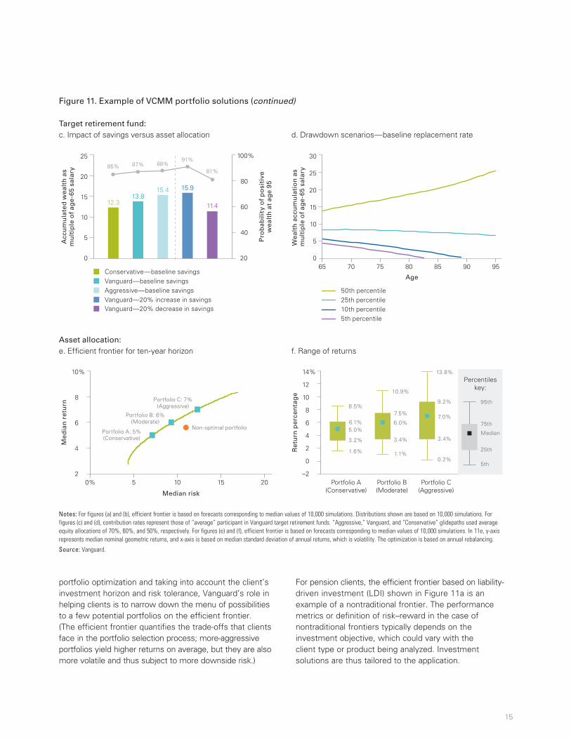
portfolio optimization and taking into account the client’s investment horizon and risk tolerance, Vanguard’s role in helping clients is to narrow down the menu of possibilities to a few potential portfolios on the efficient frontier. (The efficient frontier quantifies the trade-offs that clients face in the portfolio selection process; more-aggressive portfolios yield higher returns on average, but they are also more volatile and thus subject to more downside risk.)

For pension clients, the efficient frontier based on liability-driven investment (LDI) shown in Figure 11a is an example of a nontraditional frontier. The performance metrics or definition of risk–reward in the case of nontraditional frontiers typically depends on the investment objective, which could vary with the client type or product being analyzed. Investment solutions are thus tailored to the application.

Figure 11. Example of VCMM portfolio solutions (continued)

Target retirement fund: c. Impact of savings versus asset allocation d. Drawdown scenarios—baseline replacement rate

Pro

bab

ility

of

po

siti

vew

ealt

h a

t ag

e 95

Acc

um

ula

ted

wea

lth

as

mu

ltip

le o

f ag

e-6

5 sa

lary

Age

0

5

10

15

20

12.3

85%

13.8

87%

15.4

88%

15.9

91%

11.4

81%

25

Vanguard—20% decrease in savings

Wea

lth

acc

um

ula

tio

n a

s m

ult

iple

of

age

-65

sala

ry

0

5

10

15

20

25

30

65 70 85 908075 95Conservative—baseline savingsVanguard—baseline savingsAggressive—baseline savingsVanguard—20% increase in savings

20

40

60

80

100%

50th percentile25th percentile10th percentile5th percentile

Asset allocation: e. Efficient frontier for ten-year horizon f. Range of returns

Med

ian

ret

urn

Median risk

2

4

6

8

10%

0% 5 10 15 20

Ret

urn

per

cen

tag

e

–2

4

2

0

6

8

10

12

14%

Portfolio A(Conservative)

Portfolio B(Moderate)

Portfolio C(Aggressive)

8.5%

6.1%5.0%

3.2%

1.6%

10.9%

7.5%

6.0%

3.4%

1.1%

13.8%

9.2%

7.0%

3.4%

0.2%5th

95th

Median

75th

25th

Non-optimal portfolioPortfolio A: 5%(Conservative)

Portfolio B: 6%(Moderate)

Portfolio C: 7%(Aggressive)

Percentileskey:

Notes: For figures (a) and (b), efficient frontier is based on forecasts corresponding to median values of 10,000 simulations. Distributions shown are based on 10,000 simulations. For figures (c) and (d), contribution rates represent those of “average” participant in Vanguard target retirement funds. “Aggressive,” Vanguard, and “Conservative” glidepaths used average equity allocations of 70%, 60%, and 50%, respectively. For figures (e) and (f), efficient frontier is based on forecasts corresponding to median values of 10,000 simulations. In 11e, y-axis represents median nominal geometric returns, and x-axis is based on median standard deviation of annual returns, which is volatility. The optimization is based on annual rebalancing.

Source: Vanguard.

For sponsors of DB plans, the VCMM output provides an in-depth analysis of liability funding and duration matching. The main objective of a pension plan sponsor is to fund a plan’s expected liabilities using the plan’s assets. The model can be used to simulate possible investment portfolios that lead to different assets-to-liability (A/L) ratios for the plan. In this case, the efficient frontier can be recast in terms of A/L ratios and A/L volatilities. Portfolio duration also changes along the frontier, and thus part of the decision involves selecting portfolios with the desired duration. Figure 11a displays a sample LDI efficient frontier for a DB plan, while Figure 11b shows the terminal funding ratio for the current portfolio and portfolios in various phases of derisking the plan.

Life-cycle portfolios, such as the target retirement funds (TRFs), are constructed to decrease risk exposure over the working life of an investor in preparation for his or her retirement. The VCMM can be used to study the sensitivity of these TRFs to asset weights, saving rates, and even asset types (see Donaldson et al., 2013, for details). As an example, Figure 11c shows how the accumulated wealth varies with both the portfolio’s risk exposure and the investor’s contribution rate. For a given drawdown, the wealth accumulation or consumption can also be simulated during retirement, providing an investor with probabilistic views on investment success during retirement (see Figure 11d).

Caveats of VCMM forecasts

The VCMM is a well-designed, advanced, quantitative simulation engine, but as with any statistical model, it possesses limitations and measurement imprecision. Here, we address some concerns related to the VCMM forecasts.

Limitations of the quantitative analysis

Projections generated by the VCMM are based both on estimated historical relationships and on assumptions about the risk characteristics of various asset classes. As a result, the accuracy of VCMM forecasts depends on the relevance of the historical sample in simulating future events.

Forecasting is both an art and a science. The VCMM’s quantitative output alone will not always provide the most accurate answer. That is why Vanguard investment teams complement the model’s raw quantitative predictions with additional qualitative analysis. These qualitative overlays are based on the professional judgment and industry experience of Vanguard analysts as well as on objective, but qualitative, information. This objective information

includes expectations from market consenses, consumer-sentiment indicators, and other information from external sources not captured within the VCMM.

The interdependencies among the VCMM inputs are captured using a covariance matrix. The vector autoregression (VAR) technique used to determine these interdependencies and subsequently to simulate the asset return trajectories assumes that this covariance matrix is static. Although this assumption of “stationarity” is standard practice in industry, in reality correlations between the inputs normally vary slowly with time. This assumption could reduce the thickness of the return tails, but the VCMM compensates for these reductions in several ways. One example of this compensation is the use of non-normal innovations during the VAR forecasting process.

It’s important to emphasize that the VCMM was not designed as a short-term tactical asset allocation model. Generally speaking, portfolio analyses based on VCMM output focus on expected long-run returns over horizons equaling or exceeding ten years.

Time-dependency of VCMM long-term forecasts

The VCMM core VAR is updated quarterly and reestimated with the additional historical observation. New forecasts for the core risk factors are then launched from the recently added data point. Following the VCMM quarterly update, the core and attribution modules are reestimated. As a result, the model parameters used to generate the simulations will change.

This time-dependency of the forecasts is a strength of the VCMM because current market conditions are directly incorporated into the forecasts. And since these forecasts are initialized to current market conditions (that is, to the most current quarter of available data), simulation results are heavily influenced by the most recent data point. This influence is especially true for shorter forecast horizons.

The long-term targets built into the model are additional strengths of the VCMM. As mentioned, the output targets are founded on long-term observations, but are adjusted for structural changes in the financial markets. For example, inflation in the 1970s was much higher than what might be expected as a long-term average for the future. As such, when determining the steady state (that is, the long-term target) for inflation, we would want to moderate the effect of the high inflation levels experienced in the 1970s. Thus the long-term targets affect the steady-state behavior of VCMM outputs.

16

Conclusion

The VCMM is a proprietary model of the global capital markets that, by analyzing a broad range of options and highly tailored solutions, is designed to help clients make effective investment decisions. This paper has highlighted four key features of the VCMM asset return simulation model.

First, the VCMM explicitly accounts for current market conditions in driving forward-return distributions, and explicitly allows for time-varying risk factors and risk premiums. The long-term equilibrium conditions imposed on the VCMM are based on both quantitative and qualitative factors, which are determined by experienced analysts within Vanguard’s Investment Strategy Group.

Second, as an integrated model of the capital markets and the global economy, the VCMM combines economic and financial variables to weigh many risk factors. In this setting, investors can assess the impact of expected changes in interest rates, inflation shocks, or economic growth on their portfolios.

Third, the VCMM is forward-looking, in that, rather than relying on historical time-pathing as a way to infer future scenarios, it creates its own scenarios using outcome distributions. This distribution perspective encourages investors to consider extreme risk events that have not occurred in the recent past, but that certainly could happen within the investment horizon.

Fourth, by focusing on ranges of outcomes rather than on point forecasts, the VCMM can better incorporate statistical uncertainty into its forecasts. As we have stated, a well-reasoned approach to statistical uncertainty is an important aspect of any analytical model. This statistical uncertainty provides investors with a powerful framework to assess unanticipated risks.

References

Bernanke, Ben S., Jean Boivin, and Piotr Eliasz, 2004. Measuring the Effects of Monetary Policy: A Factor-Augmented Vector Autoregressive (FAVAR) Approach. NBER Working Paper No. 10220. Cambridge, Mass.: Harvard University.

Davis, Joseph H., 2006. Financial Simulation and Investment Expectations. Valley Forge, Pa.: The Vanguard Group.

Davis, Joseph, Roger Aliaga-Díaz, Charles J. Thomas, and Andrew J. Patterson, 2014. Vanguard’s Economic and Investment Outlook. Valley Forge, Pa.: The Vanguard Group.

Donaldson, Scott J., Francis M. Kinniry Jr., Roger Aliaga-Díaz, Andrew J. Patterson, and Michael A. DiJoseph, 2013. Vanguard’s Approach to Target-Date Funds. Valley Forge, Pa.: The Vanguard Group.

He, Ying, and Carlos I. Medeiros, 2011. An Assessment of Estimates of Term Structure Models for the United States. IMF Working Paper WP/11/247. Washington, D.C.: International Monetary Fund.

Markowitz, Harry M., 1959. Portfolio Selection: Efficient Diversification of Investments. New York: John Wiley & Sons.

Stockton, Kimberly A., 2014. Fundamentals of Liability-Driven Investing. Valley Forge, Pa.: The Vanguard Group.

17

Appendix. More about Vanguard Capital Markets Model and index details

VCMM projections and asset classes

IMPORTANT: The projections or other information generated by the Vanguard Capital Markets Model regarding the likelihood of various investment outcomes are hypothetical in nature, do not reflect actual investment results, and are not guarantees of future results. VCMM results will vary with each use and over time.

The VCMM projections are based on a statistical analysis of historical data. Future returns may behave differently from the historical patterns captured in the VCMM. More important, the VCMM may be underestimating extreme negative scenarios unobserved in the historical period on which the model estimation is based.

The Vanguard Capital Markets Model is a proprietary financial simulation engine developed and maintained by Vanguard’s Investment Strategy Group. The model forecasts distributions of future returns for a wide array of broad asset classes. Those asset classes include U.S. and international equity markets, several maturities of the U.S. Treasury and corporate fixed income markets, international fixed income markets, U.S. money markets, commodities, and certain alternative investment strategies. The theoretical and empirical foundation for the Vanguard Capital Markets Model is that the returns of various asset classes reflect the compensation investors require for bearing different types of systematic risk (beta). At the core of the model are estimates of the dynamic statistical relationship between risk factors and asset returns, obtained from statistical analysis based on available quarterly financial and economic data from as early as 1960. Using a system of estimated equations, the model then applies a Monte Carlo simulation method to project the estimated interrelationships among risk factors and asset classes as well as uncertainty and randomness over time. The model generates a large set of simulated outcomes for each asset class over several time horizons. Forecasts are obtained by computing measures of central tendency in these simulations. Results produced by the tool will vary with each use and over time.

Indexes used in our calculations

The long-term returns for our hypothetical portfolios are based on data for the appropriate market indexes through March 2014. We chose these benchmarks to provide the most complete history possible, and we apportioned the global allocations to align with Vanguard’s guidance in constructing diversified portfolios. Asset classes and their representative forecast indexes are as follows:

• U.S. equities: MSCI US Broad Market Index.

• Australian equities: MSCI Australia Index.

• U.K. equities: MSCI United Kingdom Index.

• European Economic and Monetary Union equities: MSCI EMU Index.

• Japanese equities: MSCI Japan Index.

• Emerging-markets equities: MSCI EM Index.

• Global ex-U.S. equities: MSCI All Country World ex USA Index.

• Global equities: MSCI All Country World Index.

• U.S. cash: U.S. 3-Month Treasury—constant maturity.

• U.S. Treasuries: Barclays U.S. Treasury Bond Index.

• U.S. intermediate credit bonds: Barclays U.S. Intermediate Credit Bond Index.

• U.S. aggregate bonds: Barclays U.S. Aggregate Bond Index.

• Global aggregate bonds: Barclays Global Aggregate Bond Index.

• Global aggregate ex-U.S. bonds: Barclays Global Aggregate ex-USD Bond Index.

• U.S. REITs: FTSE/NAREIT US Real Estate Index.

• Australian cash: Australian 1-Month Government Bond.

• Australian government bonds: Barclays Australian Treasury Index.

• Australian credit bonds: Barclays Australian Credit Index.

• Australian aggregate bonds: Barclays Australian Aggregate Bond Index.

• Global aggregate ex-Australia bonds: Barclays Global Aggregate ex-AUD Bond Index.

• Australian REITs: FTSE EPRA/NAREIT Australian Index.

• Global ex-Australian equities: MSCI All Country World ex-Australia Index.

• U.K. cash: UK 3-Month Gilts.

• U.K. treasuries: Barclays Sterling Gilts Index.

• U.K. credit bonds: Barclays Sterling Non-Gilts Index.

• U.K. aggregate bonds: Barclays Sterling Aggregate Bond Index.

• Global aggregate ex-U.K. bonds: Barclays Global Aggregate ex-GBP Bond Index.

• Global ex-U.K. equities: MSCI All Country World ex-UK Index.

18

19

Figure A-1. Sample set of asset classes with ten-year annualized return distribution in equilibrium

–10% –5 0 5 10 15 20 25 30

U.S. cash

U.S. Treasuries

U.S. intermediate-term credit bonds

U.S. bonds

Global bonds ex-U.S. hedged in USD

U.S. REITs

U.S. equities

Global equities ex-U.S. unhedged in USD

Australian cash in AUD

Australian government bonds in AUD

Australian credit bonds in AUD

Australian aggregate bonds in AUD

Global aggregate bonds ex-Australia hedged in AUD

Australian REITs in AUD

Australian equities in AUD

Global equities ex-Australia unhedged in AUD

U.K. cash in GBP

U.K. treasuries in GBP

U.K. credit bonds in GBP

U.K. sterling aggregate bonds in GBP

Global aggregate ex-U.K. bonds hedged in GBP

U.K. equities in GBP

Global equities ex-U.K. unhedged in GBP

Return of $1 AUD in USD

Return of £1 GBP in USD

Return of €1 EUR in USD

Return of ¥1 JPY in USD

Global bonds hedged in USD

Global equities unhedged in USD

Emerging-markets equities unhedged in USD

Percentileskey:

5th

95th

75th

25th

Notes: VCMM forecast corresponds to distribution of 10,000 simulations during years 21–30 of forecast. See the accompanying appendix section “Indexes used in our calculations,” for details of indexes used for each asset class.

Source: Vanguard.

Connect with Vanguard® > vanguard.com

For more information about Vanguard funds, visit vanguard.com, or call 800-662-2739, to obtain a prospectus. Investment objectives, risks, charges, expenses, and other important information about a fund are contained in the prospectus; read and consider it carefully before investing.

CFA® is a registered trademark owned by CFA Institute.

© 2014 The Vanguard Group, Inc. All rights reserved. Vanguard Marketing Corporation, Distributor.

ISGGCM 112014

Vanguard Research

P.O. Box 2600 Valley Forge, PA 19482-2600