Electronic copy available at: http://ssrn.com/abstract=2084180

Valuing high technology growth firms*

Soenke Sievers†, Jan Klobucnik#

This draft: June 14, 2012

Abstract For the valuation of fast growing innovative firms Schwartz and Moon (2000, 2001) develop a fundamental valuation model where key parameters follow stochastic processes. Guided by eco-nomic theory, this paper is the first to design a large-scale applicable implementation on around 30,000 technology firm quarter observations from 1992 to 2009 to assess this model. Evaluating the feasibility and performance of the Schwartz-Moon model reveals that it is on average compa-rably accurate to the traditional sales multiple with advantages in valuing small and non-listed firms. Most importantly, however, the model is able to indicate severe market over- or underval-uation. Consequently, a trading strategy based on our implementation has significant investment value. JEL classification: G11, G12, G17, G33 Keywords: Schwartz-Moon model, market mispricing, empirical test, company valuation, trading strategy

* We are very grateful to Georg Keienburg for his insightful suggestions and valuable comments. This paper has also benefited from the comments of Jeff Abarbanell, John Hand, Dieter Hess, Thomas Hartmann-Wendels and seminar participants at the 2012 Midwest Finance Association Meeting, the 2012 European Accounting Association Annual Congress and the 2012 German Academic Association for Business Research Meeting. #Cologne Graduate School, Richard Strauss Strasse 2, 50923 Cologne, Germany, e-mail: klobucnik@wiso.uni-koeln.de, phone: +49 (221) 470-2352 †(Corresponding author) Accounting Area, c/o Seminar für ABWL und Controlling, Albertus Magnus Platz, Univer-sity of Cologne, 50923 Cologne, Germany, e-mail: sievers@wiso.uni-koeln.de, phone: +49 (221) 470-2352

Electronic copy available at: http://ssrn.com/abstract=2084180

1

1. Introduction

Web based social networks like Facebook, Twitter and so forth are currently one of the fastest

growing industries and therefore attracting investors’ attention. Recently, Facebook went public

as the second-largest U.S. IPO of all time, implicitly valuing this company at around $100 bil-

lion. The result was a market capitalization higher than for mature internet firms as Ebay or Am-

azon.1 While Facebook’s IPO currently dominates the media, its social network game develop-

ment company Zynga, the deal-of-the-day website Groupon and the music recommendation ser-

vice Pandora went public last year with corresponding firm values of $13 billion, $7 billion and

$2 billion, respectively, although still making losses.2 Hence, the challenging exercise of valuing

fast growing technology firms is becoming popular again despite the recent financial crisis.

In response to the demand for a valuation model suitable for such firms, Schwartz and Moon

(2000) and Schwartz and Moon (2001) develop and extend a theoretical model explicitly focus-

ing on the value generating process in high technology growth stocks. It is based on fundamental

assumptions about the expected growth rate of revenues and the company’s cost structure to de-

rive a value for technology firms. Using simple Monte Carlo techniques and short term historical

accounting data, the Schwartz-Moon model simulates a growing technology firm’s possible

paths of development. As next step, it calculates a fundamental firm value by averaging all dis-

counted, risk-adjusted outcomes of the simulated enterprise values. Additionally, throughout the

growth process firms may default. Therefore, the model provides investors not only with a value

estimate but also with a long term probability of bankruptcy, which is not the case for the stand-

ard valuation procedures such as multiples. Another major advantage is that it does not require

market data which makes it applicable for the large number of non-listed firms. Finally, given

that high technology firms often experience losses and do not have analyst coverage, one has to

take into account that the most accurate valuation methods, as Discounted Cash Flow (DCF)

models or price earnings multiples, are not applicable. Due to its theoretical appeal, the model

has been used and extended by other studies like Pástor and Veronesi (2003, 2006) or Schultz

and Zaman (2001). Surprisingly, however, the original model has never been tested on a large

1 Wall Street Journal (05/17/12): Facebook Prices IPO at Record Value. 2 Reuters (11/04/11): Groupon's IPO biggest by U.S. Web company since Google. Wall Street Journal (01/17/12):

Zynga Chief Talks IPO, Lessons Learned. Wall Street Journal (06/11/11): Pandora Raises IPO's Size.

2

scale before.

Based on these thoughts, the issue arises whether the theoretical Schwartz-Moon model can

fill this gap in the valuation literature, despite the difficulty that many of the model's input pa-

rameters need to be estimated ex-ante. Specifically, we ask the following three research ques-

tions: First, given the theoretical advantages but challenging input parameter estimation of the

Schwartz-Moon model, how does an economic reasonable, but at the same time feasible imple-

mentation look like? Second, how does the proposed model implementation perform in terms of

valuation accuracy? Third, given that the model is based on fundamental accounting information,

is it possible to indicate market misvaluation in the technology sector?

Answering these questions yields the following key results: First, building on economic theo-

ry regarding the development of key accounting and cash flow figures in a competitive market

environment, we present an easily applicable configuration of the Schwartz-Moon model. It is

developed for large scale valuation purposes on a sample of around 30,000 technology firm quar-

ter observations from 1992 to 2009 using realized accounting data. Second, although this model

is especially suited for non-listed firms, we need the market environment to test its feasibility.

Therefore, we compare the fundamentals based Schwartz-Moon model to the Enterprise-Value-

Sales method and find that it performs on average comparably accurate with regard to deviations

from market values. Moreover, there are clearly smaller valuation errors for firms in the chemi-

cals and computer industries and for smaller companies. Note that this perspective assumes that

markets are on average efficient considering the complete time period and are not influenced by

market sentiment. Finally and most importantly, leaving this accuracy perspective and turning to

the last question of potential misvaluation, the Schwartz-Moon model shows the ability to indi-

cate severe market over- or undervaluation in each quarter from 1992 until 2009 and to produce

reasonable estimates for the probability of default. Given these findings, we demonstrate that a

trading strategy based on the Schwartz-Moon model has significant investment value, both be-

fore and after transaction costs.

By providing and testing an applicable implementation of the Schwartz-Moon model, we

contribute to the literature on company valuation. Our findings offer promising results on how to

accurately value especially small firms, which often exhibit losses and are therefore excluded in

3

other studies.3 Furthermore, these firms are often not covered by analysts; consequently, other

fundamental valuation models as the discounted cash model are not applicable. Including analyst

forecasts would lead to an important sample selection bias as demonstrated in Pástor and

Veronesi (2003).4 Moreover, even if analyst forecasts are available, they are frequently overop-

timistic as demonstrated in Easterwood and Nutt (1999). This would then contradict the effort to

detect misvaluation. In contrast, the Schwartz-Moon model only relies on a short history of eight

quarters of firm-specific accounting data. Although it contains more than 20 parameters, we in-

troduce a sensible implementation, which is only based on major items from the income state-

ment and the balance sheet and information about firms in the same industry, thereby significant-

ly reducing the model’s complexity. Furthermore, it is also applicable to non-publicly traded

firms and does not rely on market prices. This can be of special interest during times of ineffi-

cient markets and for investors who target unlisted firms and in particular for venture capital and

private equity investors who invest in small to medium technology enterprises as documented in

Cumming et al. (2005).

Following the compelling logic of rational pricing, the original model intends to rational-

ize high stock prices during the dot-com bubble. Nevertheless, Schwartz and Moon (2000, 2001)

are not able to explain the high stock prices rationally as they would need implausibly high vola-

tility estimates. Building on this approach, Pástor and Veronesi (2006) relate extreme valuations

to uncertainty. They argue that market valuations could be justified during the dot-com bubble;

however they assume a period of 15 years of abnormal profits, which seems quite high in a com-

petitive environment. Therefore, by focusing on matching valuation estimates to observed mar-

ket values, one might overlook the clear advantages of the model compared to the multiple

benchmark. It is well documented in the literature that, first, valuations are highly influenced by

market sentiment (see, for example, Inderst and Mueller 2004 or Bauman and Das 2004) which

can, second, lead to misvaluations and bubbles (Baker and Wurgler 2007 or Stambaugh et al.

2012). Therefore, regarding the first aspect, our benchmark for the model’s accuracy to market

values, the Enterprise-Value-Sales multiple (EV-Sales), should naturally yield smaller valuation

3 In fact, taking a closer look at recent valuation model accuracy studies such as Liu et al. (2002), Bhojraj and Lee

(2002) or Eberhart (2001), most of them exclude all firms that do not fulfill criteria such as positive earnings, an-alyst coverage, share price larger than $3 and minimum sales of $100 million.

4 Requiring basic analyst data as 1-year-, 2-year-ahead sales and gross margin forecasts for our sample firms would reduce our sample by over 60%.

4

errors as it captures the market sentiment. Nevertheless, we need the market environment to

check the feasibility of our implementation and it indeed results in comparable accuracy. Put

differently, while the Schwartz-Moon model is purely based on historical accounting data, multi-

ples are generally calibrated to capture the current market mood by explicitly relying on the mar-

ket values of competitor firms. However, this independence of current market sentiment allows

the fundamentals based Schwartz-Moon model to detect periods of severe market mispricing,

which is in line with the second aspect mentioned above. Consequently, we hypothesize that

market valuations can be unjustified during bubble times and add to the literature which indicates

that the financial accounting data can serve as an anchor for rational pricing during these times as

in Bhattacharya et al. (2010). This is especially true for technology growth firms whose valua-

tions are highly subjective and therefore strongly affected by investor sentiment as documented

in Baker and Wurgler (2006). Consequently, we provide additional evidence that a trading strat-

egy based on our model implementation of Schwartz-Moon has economic and statistically signif-

icant investment value, both before and after transaction costs. Risk adjusted abnormal returns

before transaction costs are as high as 1.5% per month.

The remainder of this paper is structured as follows. In section 2 we provide an overview of

the related literature and discuss the properties of technology growth firms in the context of firm

valuation. Section 3 discusses the Schwartz-Moon model and introduces the benchmark valua-

tion procedure. Section 4 describes the sample and model implementation. In section 5 we em-

pirically investigate the model’s performance and section 6 presents the robustness checks. Fi-

nally, section 7 concludes.

2. Related literature: Firm growth and valuation

In this section we briefly discuss the relevant valuation literature with a focus on technology

growth companies. To start with, we discuss the “nifty fifty”. They were the high-flying growth

stocks of the 1960s and early seventies. These companies, including General Electric, IBM, Tex-

as Instruments and Xerox were the growth firms of their time. Due to their notably high valua-

tions, those firms were later compared to new economy stocks enjoying tremendous high valua-

tions in the late 1990s as stated in Baker and Wurgler (2006). Still, while the “nifty fifty” were

strongly growing companies, their valuation was based on the ability to generate rapid and sus-

5

tained earnings growth and persistently increase their dividends. In addition, those firms were

already well established large cap entities, thereby confirming Gibrat’s rule and the theoretical

models of Simon and Bonini (1958) and Lucas Jr. (1967) that assume growth to be independent

from firm size. Consequently, growing firms could easily be valued using standard valuation

methods such as the discounted cash flow model with analyst forecast data or the Price-Earnings-

Ratio with a sufficient peer group as in Cheng and McNamara (2000).

The tremendous rise in high technology stock prices during the end of the 1990s and its sub-

sequent fall throughout the early years in the new century, known as the dot-com bubble, let the

economics of technology firms gain significant attention again. Practitioners and researchers

began to realize that internet stocks are a chaotic mishmash defying any rules of valuation.5

Starting to question the relation between financial ratios and equity value of stocks, as docu-

mented by Core et al. (2003), Trueman et al. (2000) analyze new measures of technology firm

value drivers such as customer’s internet usage. In a more general approach, Zingales (2000)

describes the appearance of a new type of firm based on new technology. He finds three factors

to disturb existing firm theories: Reduced value generation by physical assets, increased compe-

tition and the importance of human assets. But why would new technology have influence on

firm valuation approaches?

McGrath (1997) relates investments in high technology firms with real options logic. In her

framework, the value of the technology option is the cost to develop the technology. Completing

the development of the technology will create an asset which is the underlying right of the firm

to extract rents from the technology. This gives three insights.

First, growing technology firms might exhibit losses as they face costs of development, but

no yet marketable products. In this context, Demers and Lev (2001) argue that high technology

firms require significant up-front capital to establish their technological architecture. In line with

this argument, Bartov et al. (2002) find that since the 1990s, innovative high technology firms

are expected to grow rapidly, while they are still not profitable. In this study we will present a

sample of 29,477 technology firm quarter observations with median annual sales of 142$m and a

significant share (34%) of negative earnings observations. Consequently, we conclude that recent

studies on valuation model accuracy do not include a significant share of high technology com-

5 Wall Street Journal (12/27/99): Analyst Discovers the Order in Internet Stocks Valuation.

6

panies.

Second, from a stock market perspective, high technology growth firms have specific

characteristics. Their stocks are exposed to severe volatility as documented in Ofek and Richard-

son (2003), which makes it difficult to determine the underlying value. At the same time, there is

a strong influence of investor sentiment on the value of technology firms found in Baker and

Wurgler (2006) or Inderst and Mueller (2004). Hence, relative valuation methods, i.e., multiples,

for high technology firms are heavily influenced by the current mood of the market. Compared to

fundamentally based valuation models as DCF, the multiples should not be able to make any

statements about overall market over- or undervaluation. Consequently, valuation methods based

on financial statement information should therefore have the potential to serve as rationale

benchmark during volatile and speculative market periods. This is especially important as prices

reflect fundamentals in the long run as presented in Coakley and Fuertes (2006).

Third, the risk of the new technology failing can result in bankruptcy. Thus, the risk of

default plays a more central role in valuation of high technology firms. Vassalou and Xing

(2004) and Kapadia (2011) report default risk to be a relevant factor for explaining equity re-

turns. Beside the general fact that bankruptcy is costly and negatively affects small and large

investors, information on default risk is especially important for under-diversified investors.

Cumming and MacIntosh (2003) and Cumming (2008) document tremendous default risks with

failure rates of 30% for portfolios that are specialized in young entrepreneurial firms. These re-

sults show that valuation models -especially with regard to small companies- should incorporate

default risk explicitly. Since this is the case in the Schwartz-Moon framework, this model is

preferable to standard approaches, which are typically working on a going concern basis.

In sum, we see that standard valuation procedures are less applicable for high technology

firms, which are especially influenced by market mood and exposed to default risk. The firms in

our sample are likely comparable to young and growing venture backed firms. In this context,

Hand (2005) and Armstrong et al. (2006) find that traditional accounting measures such as bal-

ance sheet and income statement are able to explain variation in market values for venture capital

backed growing technology firms. Taking these specifics into account, the Schwartz-Moon mod-

el might offer a way to determine a fundamentally justified value of high technology growth

firms. In the following we present the original model.

7

3. Valuation models

3.1. Fundamental pricing: The Schwartz-Moon model

The Schwartz-Moon model (2000, 2001) is most easily explained in the context of traditional

valuation models, such as the familiar discounted cash flow model, where the cash flow to equity

(FTE) is discounted at an appropriate risk adjusted cost of equity as in Francis et al. (2000). For

all these models, one of the most challenging tasks is the derivation of future payoffs. While

there are several ways to tackle this problem, the most sensible method is to forecast future bal-

ance sheets and income statements and derive the necessary payoff-figures as in Lundholm and

O'Keefe (2001). Following this logic, one needs forecasts for the basic financial statement items

as shown in the next two figures.

-----------------Please insert Figure 1 approximately here-----------------

-----------------Please insert Figure 2 approximately here-----------------

Since analysts' forecasts for high technology firms are often not available, the commonly applied

forecasting technique is the percentage of sales method. Here, one explicitly focuses on revenues

forecasts and the other value relevant parameters are tied to these forecasts based on a historical

ratio analysis as applied in Nissim and Penman (2001). The revenues forecasts are influenced by

many parameters, such as industry dynamics or actions from competitors. Consequently, after

some finite forecast horizon, it is reasonably assumed that initially high growth rates of revenues

will converge to average industry levels. Finally, the company will achieve a mature, steady-state

status and revenues grow with the industry rate. The convergence to industry levels is theoreti-

cally well established as in Denrell (2004) and commonly applied in empirical studies concerned

with company valuation such as Lee et al. (1999).

The Schwartz-Moon model is exactly based on these thoughts, since it models the value driv-

ing input parameters given by the income statement and the balance sheet with stochastic pro-

cesses. Below, we present the model as introduced by Schwartz and Moon (2001).

Following the percentage of sales method, revenue dynamics (R) are given by the stochastic

differential equation:

8

��(�)�(�) = ��() − �� ∙ ()�� + () ∙ ���() (1)

where the drift term ( )tµ represents the expected growth rate in revenues and ( )tσ is the growth

rates’ volatility. Unanticipated changes in growth rates are modeled by the random variableRz ,

following a Wiener process. The risk adjustment term λR accounts for the uncertainty and allows

for discounting at the risk free rate later. With time t, the initial growth rates converge to their

long term growth rateµ following a simple Ornstein-Uhlenbeck process.

��() = ���(� − �()) − �� ∙ �()�� + �() ∙ ���() (2)

where µκ denotes the speed of convergence and ( )tη is the volatility of the sales growth rate.

Different from Schwartz and Moon (2001), we do not make the simplifying assumption that the

true and the risk adjusted revenues growth processes are the same, which is why we introduce

the risk adjustment term λµ. Unanticipated changes in revenues ( )tσ converge with σκ to their

long-term averageσ , while the volatility of expected growth ( )tη converges to zero.

( ) ( )d t t dtσσ κ σ σ= ⋅ − (3)

( ) ( )d t t dtηη κ η= − ⋅ (4)

Summing up, the two main parameters of the revenue process (growth rate ( )tµ and the growth

rates’ volatility ( )tσ ) exhibit the desirably property of long term convergence justified by a

competitive market environment.

Turning to the second item on the income statement, cost dynamics C(t) are modeled based

on two components. The first component is variable cost dynamics ( )tγ , which is proportional to

the firm’s revenues. The second component is fixed costs F.

( ) ( ) ( )C t t R t Fγ= ⋅ + (5)

Again, cost dynamics are assumed to converge to their industry levels according to the following

mean-reverting process:

��() = ���(� − �()) − �� ∙ �()�� + �() ∙ ���() (6)

9

where γκ denotes the speed of convergence at which variable costs ( )tγ converge to their long

term average γ . Here we also adjust for the uncertainty by adding the risk adjustment term λγ.

Unanticipated changes in variable costs are modeled by ( )tϕ , converting deterministically with

ϕκ against long term variable cost volatilityϕ .

[ ]( ) ( )d t t dtϕϕ κ ϕ ϕ= ⋅ − (7)

As Schwartz and Moon (2001) suggest, it is reasonable to assume the three speed of adjustment

coefficients to be the same, leaving us with one single κ. Dividing log(2) by κ yields the half-life

of the processes, which can easily be interpreted.6 While revenues and costs are modeled inde-

pendently from the balance sheet, the development of property, plant and equipment PPE(t) de-

pends on the development of capital expenditures CE(t) and depreciation D(t). The former value

is assumed to be a fraction cr of revenues while depreciation is assumed to be a fraction dp of the

accumulated property, plant and equipment. Consequently, both financial statements are linked

consistently to each other by:

[ ]( ) ( ) ( )dPPE t D t CE t dt= − + (8)

Finally, taxes and the dynamics of loss carry forwards are considered by Schwartz and Moon

(2001). Since firms can offset initially negative earnings with future positive earnings for tax

purposes, we calculate loss carry forward dynamics as:

[ ] [ ][ ]

( ) ( ) , ( ) ( ) ( )( )

max ( ) ,0 ,

Y t Tax t dt if L t Y t Tax t dtdL t

L t dt else

− + > += −

(9)

Controlling for tax payments Tax(t) and loss carry forwards L(t), the after tax income ( )Y t in the

Schwartz-Moon model is given by:

( ) ( ) ( ) ( ) ( )Y t R t C t D t Tax t= − − − (10)

Assuming that no dividends are paid and positive cash-flows are reinvested, earning the risk-free

rate of interest r, the amount of cash available to the firm X evolves according to:

[ ]( ) ( ) ( ) ( ) ( )dX t r X t Y t D t CE t dt= ⋅ + + − (11)

6 Assuming exponential decay, the half-life can be derived by solving the following equation for �:���� = !

".

10

Firms fail when their available cash falls below a certain threshold X* and the enterprise value is

set to the liquidation value of PPE plus the (negative) cash. Otherwise, the model implied fun-

damental value at time t is calculated by discounting the expected value of the firm at time T

under the risk neutral probability measure Π with the risk free rate r, as the three stochastic pro-

cesses are corrected for uncertainty by the risk premiums λR, λµ and λγ. The firm’s enterprise val-

ue consists of two components. The cash amount outstanding and, second, the residual company

value, which is calculated as EBITDA = R(T)-C(T) times a multiple M.

#$(0)& = #'()(*) + + ∙ �,(*) − -(*)�. ∙ ��/∙0 (12)

The assumptions of no dividend pay-out, no explicit modeling of tax-shields due to the deducti-

bility of interest payments and the solution of the terminal value problem via an exit multiple

deserve discussion. While it seems restrictive at first glance, the model is basically employed in a

Modigliani and Miller (1958) framework, since it assumes that it does not matter whether equity-

owners or the firm holds cash. Furthermore, within the branch of literature concerned with capi-

tal structure choice, such as Miller (1977) and Ross (1985), one can argue that advantages and

disadvantages of debt financing balance, so it might be a simplifying but justifiable assumption,

that the financing decision is not considered explicitly in the Schwartz-Moon model.

Concerning the terminal value problem, it should be noted, that the finite forecast horizon

is chosen to be 25 years as in Schwartz and Moon (2001). Consequently, the calculated terminal

value plays only a minor role as shown in the robustness section.

3.2. Introducing a benchmark: Enterprise-Value-Sales-Multiple

The Schwartz-Moon model implementation is based on the principles of historical, fundamental

valuation. Therefore, the natural counterpart would be based on a DCF model. As argued earlier,

we want to abstract from analyst forecasts and, additionally, the technology firms in our sample

often lack analyst coverage. Hence, these input parameters for the DCF model in the large and

therefore anonymous dataset are not an option. Alternatively, we turn to relative financial ratios

referred to as multiples to provide a sanity check for the magnitude of valuation errors for our

Schwartz-Moon model test.

Multiples are widely used in practice by consultants, analysts and investment bankers as

shown for example by Bhojraj and Lee (2002). Among other traditional valuation methods, such

11

as traditional DCF-models, they generally produce the smallest valuation errors as shown by Liu

et al. (2002) and Bhojraj and Lee (2002). Thus, we choose to compare the Schwartz-Moon model

against this very accurate valuation method. As noted beforehand, there are many multiples

available (Price-Earnings, Price-Book, Price-Sales etc.) and they can be implemented in many

different ways (simple peer-group comparison vs. sophisticated regression approach). Conse-

quently, we have to choose among these many possibilities. Given the fact that our study is con-

cerned with technology growth firms, many of them have negative earnings or even negative

EBITDA. Hence, standard multiples such as Price-Earnings or Enterprise-Value-EBITDA are

not applicable. At the same time, we look for a comparable measure which comes close to the

idea of the Schwartz-Moon model with the major driving force being sales from its stochastic

processes. Since six of the seven critical parameters we identify below depend on sales, our

choice is naturally guided to the Enterprise-Value-Sales Multiple. Thus, it provides a reference

point to assess the magnitude of valuation errors.

The Enterprise-Value-Sales method evaluated in this paper follows Alford (1992), where

a firm i’s value is estimated by the product of firm i's sales at τ and the median of the j peer

group's (PG) EV-Sales multiples.

#$()& 1 = 234�5(6)1 ∙ 7��839:∈<=> ? @A(�)BCDEFG(H)BI (13)

where enterprise value (EV) is the market value of equity plus the book value of debt. Note that

#$J is the estimated value whereas EV simply denotes observable information. A key component

in relative pricing is the identification of comparable companies. Alford (1992) and Cheng and

McNamara (2000) examine the effects of comparable company selection on relative valuation

accuracy and find that comparable companies selected on industry classification and additional

measures such as profitability yield the lowest estimation errors. Therefore, we perform EV-

Sales Multiple valuations based on four digit SIC code industry classifications. Within the indus-

try we group firms by their return on net operating assets (RNOA) to account for profitability

effects (cf. appendix 1). That is, we choose those six firms that are closest to firm i's RNOA

within the preceding year. If fewer than six companies are available in this SIC code classifica-

tion, we relax this requirement to companies with the same three and two digit SIC code. The

12

peer group median then is calculated to obtain the multiple. The product of the multiple and the

firm’s sales yields the estimated enterprise value.

4. Data and methodology

4.1. Data collection

To construct our sample of high technology firms, we merge the CRSP database for market data

with Compustat North America quarterly and yearly accounting data. In order to calculate indus-

try specific long-term parameter values, we use the complete data set starting 1970 (cf. Appendix

1).7 However, our main sample considers all firms that fall under the Bhojraj and Lee (2002)

high technology industry SIC code definition beginning in 1992 until 2009.8 That is biotechnolo-

gy (SIC codes 2833-2836 and 8731-8734), computer (3570-3577 and 7371-7379), electronics

(3600-3674) and telecommunication (4810-4841). We add SIC code 7370 (Computer Program-

ming, Data Process) in order to keep firms such as Google or Lycos in our sample. We exclude

all firm observations with negative sales, variable costs, capital expenditure and negative enter-

prise values. This leaves us with 2,262 individual firms covering 29,477 quarters in total as can

be found in Table 1 in the appendix.

4.2. Model implementation

The most challenging issue in applying the Schwartz-Moon model is parameter estimation as

noted in Schwartz and Moon (2000). Unlike an investment banker who has detailed information

about the firm’s development, recent m&a activity and strategy decisions, we are valuing a rather

anonymous sample of around 30,000 firm quarters. Therefore, our analysis is primarily based on

short term historical accounting information, which is the common information set left for these

firms.

The Schwartz-Moon model includes 22 different input parameters. While most parameters

are estimated on a firm level basis, the long term parameters are determined on industry levels

(i.e., three digit SIC codes). Including information from comparable firms from the same indus-

7 These parameters are the long term variable costs, the long term volatility of variable costs, the capital expendi- ture rate and the depreciation rate. 8 We start with the first quarter 1992 since we need eight quarters of accounting information from 1990; since then

data availability is reasonably complete for all required items. Moreover, it sufficiently covers the inception of the industry as well as the peak and burst of the dot com bubble as described in Bhattacharya et al. (2010).

13

try decreases the volatility of estimated firm values as shown in Eberhart (2001) and hence yields

better estimates. From the perspective of importance, the 22 parameters can be divided into criti-

cal and uncritical parameters. The uncritical parameters primarily include initial values for bal-

ance sheet items where the estimation is straightforward. The critical parameters with a larger

impact on the simulation results come from the revenue and the cost processes because these two

processes are the main drivers for a firm’s EBIT. More precisely, the seven critical parameters

are estimated from quarterly financial statements’ sales and costs information and the industry

comparison, thereby significantly reducing the complexity of the model. The estimation of the

seven critical parameters is presented in the next two paragraphs and their impact is shown in the

sensitivity analysis in section 5.

4.2.1. Implementing revenue dynamics

Recall that key input parameters for the firm’s revenues are given in equation (1) to (4). Thus,

we take the initial sales R(0) as quarterly sales from quarterly accounting statements provided by

Compustat for each firm. Initial sales volatility σ(0) is calculated using the standard deviation of

sales change over the preceding seven quarters and converges to the long term quarterly volatili-

ty K= 0.05 consistent with Schwartz and Moon (2001). Further, they argue that initial expected

sales growth µ(0) should be derived using past income statements and projections of future

growth. Many private shareholders or institutional investors targeting small capitalized growth

firms will find it difficult to obtain analyst forecasts. In addition, requiring the availability of

I/B/E/S forecasts in particular excludes small firms as noted by Liu et al. (2002). However, to

value this type of firms is exactly our aim. Therefore, we do not require any analyst coverage and

derive µ(0) as average sales growth over the prior seven quarterly income statements. While this

is notably a weak proxy for future revenues growth, it is information commonly available for all

technology firms and therefore easy to apply. Additionally, Trueman et al. (2001) show historical

revenues growth to have incremental predictive power over analysts’ forecasts for internet firms.

Long term sales growthµ is set equal to 0.75% percent per quarter, which corresponds to an

assumed long term average annual inflation rate of three percent. Initial volatility of expected

growth rates in revenues (0)η is estimated firm specifically by the standard deviation of the re-

14

siduals from an AR(1)-regression on the growth rates, which is similar to the approach of Pástor

and Veronesi (2003) to estimate the volatility of profitability.

Different from Schwartz and Moon (2001) who set the speed of adjustment coefficients κ

exogenously to 0.1, we allow for mean reverting processes with industry specific (two digit SIC)

kappas. The rationale behind this approach are common factors, which drive the competitive

advantage periods within the same industries as analyzed in Waring (1996). Schwartz and Moon

(2001) argue that the kappa of the revenues growth rate process has the highest impact. Thus, we

calculate the adjustment coefficient κ with the help of revenue dynamics by solving the follow-

ing equation:

L GDEFM>�GDEFM>NOGDEFM>NO =��P1Q��R SL GDEFM>�GDEFM>NOGDEFM>NO

��T1Q��! U ∙ ��T∙�V (14)

As justified above, the estimated firm specific kappas then are pooled to medians for the same

two digit SIC codes. We choose two digit over three digit SIC levels to decrease the large varia-

tion in this critical parameter. Still, this estimator generates outliers and yields us a range of es-

timated kappas corresponding to half-lives from one to 70 quarters. In order to avoid the influ-

ence of extreme estimates of the kappas corresponding to unreasonable high half-lives, we

winsorize these variables at the 1% and 99% percentiles. As the kappas directly influence ex-

pected future revenues and costs, the speed of adjustment parameters are crucial for the three

stochastic processes.

4.2.2. Implementing cost dynamics

Recall that the input parameters for the cost dynamics are given in equation (5) to (7). Schwartz

and Moon (2001) propose to calculate costs using a regression of costs on revenues, where the

intercept represents constant fixed costs and the slope is the initial variable costs. On a large

scale application, this leads to cases in which the intercept becomes negative. Those firms would

exhibit negative fixed costs, an extremely steep slope and unreasonably high variable costs.

Therefore, we deviate from this approach, calculating the variable costs (0)γ as the average over

the preceding eight quarters of variable costs plus fixed costs divided by revenues. In doing so,

we ensure costs to be within reasonable levels. Including fixed costs into this approach assumes

that fixed costs grow linearly with firm growth. This might be a weak assumption but seems to

15

be more reasonable than assuming independence from growth. The firm’s long term cost ratio γ

is calculated based on the long term industry median. For each one digit SIC industry, we calcu-

late a growing window median costs ratio beginning in 1970 and up to 2009. Valuing firm i at

time t, we use firm i’s industry’s long term median cost ratio until time t-1 as the expected long

term costs. As costs directly determine a firm’s profit, both the initial and the long term cost pa-

rameters are crucial and strongly affect the results. The initial volatility of costs φ0 is obtained by

running firm specific AR(1) regressions on the cost ratios and calculating the standard deviation

of the residuals. Long term volatility of variable costs �W is determined as a growing window in-

dustry median cost ratio on a three digit SIC code level starting 1970. Finally, we assign the in-

dustry specific medians of the estimated standard deviations to the individual firms. This is con-

sistent with assuming similar developments within industries.

In the following, we present the uncritical parameters, which do not affect estimated firm

value results largely.

4.2.3. Implementing balance sheet and the remaining income statement items

Recall that the input parameters for the balance sheet and the remaining income statement items,

such as depreciation, are given in equation (8), (9) and (11). Initial property, plant and equipment

PPE(0) is calculated as Compustat items for net property plant and equipment plus other assets.

Due to acquisition activity and other expansion related investments, capital expenditures and

depreciation ratios are extremely noisy for growing firms. The use of a constant investment and

depreciation rate based on historical accounting information might therefore lead to biased re-

sults. To overcome biases of expansion related one time effects, we model firm i’s constant rates

of investment cr and depreciation dp as the long term industry median. For firm i’s cash and cash

equivalents X at time t, we calculate the sum of Compustat items for cash, total receivable minus

accounts payable, other current assets and treasury stock.

4.2.4. Implementing environmental and risk parameters

In line with Schwartz and Moon (2000, 2001) and given the long term interest rate from the Fed-

eral Reserve, we use for simplicity the risk free rate of 5.5% p.a. which translates to 1.35% per

quarter. However, as shown by an intensive sensitivity analysis in the robustness section, it does

16

not drive the results. Corporate tax rates are 35% as in Bradshaw (2004). The risk premium for

each of the stochastic processes �1 (i= R, µ, γ) is calculated as:

X/Y,1 ∙ /Y = [\](/Y,1)^> (15)

where rM is the return of the Nasdaq Composite Index over the preceding seven quarters and /_

is the Nasdaq Composite Index standard deviation. Thereby, as mentioned earlier, we can use

one risk free rate for discounting for all firms.

4.2.5. Implementing simulation parameters

For each valuation, we use 10,000 simulations with steps of one quarter and up to 25 years. At

the end of the simulation horizon, the enterprise value is given by the time t=100 cash value plus

the residual value EBITDA multiplied with 10 in line with Schwartz and Moon (2001). A firm

fails at any given time t=s, wheres [1;100]∈ , within the simulation horizon when the available

cash falls below zero. The liquidation value then is given as:

#$C aEbM& = ?cc#G +)G,8d − )G < cc#G0,�45� f (16)

where PPES is the amount of property, plant and equipment at default plus the negative cash XS

available. The Schwartz-Moon model estimated enterprise value is calculated by averaging all

10,000 simulated enterprise values and discounting the average value to time t=0.

4.3. Summary statistics

Table 2 reports summary statistics for our sample.

-----------------Please insert Table 2 approximately here-----------------

Panel A, Table 2, shows the industry distribution primarily based on the SIC code classification

by Bhorjraj and Lee (2002). The largest group is computer firms, accounting for 40% of our

sample. Other major industries are electronics (31%), biotechnology (18%) and telecommunica-

tions (11%). Panel B, Table 2, reports financial statement information. For convenience, we re-

17

port flow items from the income statement as annualized values calculated as the sum over four

quarters. On average, firms report annual revenues of $1.8 billion. A median revenue figure of

$142 million shows the existence of extreme upscale outliers and the small firm structure of our

sample. Median cash and cash equivalents holdings is $72 million, while we also find some

firms with negative cash holdings. This is the case for firms where the accounts payable exceeds

the sum of cash, treasury stock and receivables, but this only occurs in 1% of the observations.

Median total assets are $170 million. The large asset variation, with the smallest firm reporting

total assets of less than $1 million and the largest firm with assets above $280 billion, shows sig-

nificant heterogeneity within the sample. Median leverage, calculated as interest bearing debt

scaled by total assets, is 7%. As expected, we find debt financing to be only a minor security

choice for technology growth firms. Within 34% of all observations, the underlying firm report-

ed negative earnings and therefore profitability oriented multiples, such as Price-Earnings, can-

not be considered. Median annual earnings are 4 $m, while we also face extreme upside and

downside outliers. Even taking EBIT into account as a profitability measure, 28% of all firm

quarter observations report negative profits. Panel C, Table 2, reports summary statistics for the

seven critical parameters used within the Schwartz-Moon approach. On average, firms exhibit

mean annual sales growth rates of 29% over the preceding 7 quarters, while we also face several

annual growth rates of more than 1,000% percent. The mean initial cost ratio, calculated as total

costs scaled by sales, is 91%, while maximum values are up to 150%. This indicates the growth

firm's potential to reduce costs over time to increase profitability in the long run. The long term

cost ratio is calculated using a growing window approach based on three digit SIC industry clas-

sifications to capture industry specific characteristics. While being on comparable median levels

to initial costs, this approach assures less volatile long term cost structures indicated by the sig-

nificantly reduced inter quartile range. The long term annual revenues growth is exogenously set

to a 3% inflation rate. The initial volatility of revenues growth rate has a median of 5%, while the

corresponding measure for the initial volatility of variable cost ratio is 8%. The latter also has a

higher variability pictured by an inter-quartile range of twice the growth rate’s initial volatility.

Finally, the speed of convergence has a median of 17% corresponding to a half-life for the sto-

chastic processes of 4.1 quarters. Panel D, Table 2, reports market values. Market capitalization

is considered four months following the date the underlying financial statement refers to. This

18

way we verify that financial statement information was available to market participants by the

time we analyze market values.9 Overall, the median enterprise value in our sample is $321 mil-

lion calculated as the sum of market capitalization provided by CRSP plus long term debt and

debt in current liabilities.

5. Main empirical results

Feasibility and valuation errors

Prior studies generally report valuation accuracy based on logarithmic errors as in Kaplan and

Ruback (1995) or percentage errors such as Francis et al. (2000). For comparison, we report both

error measures in Table 3 to shed light on our research question regarding overall valuation accu-

racy. Absolute log errors are defined as the ratio of the estimated value to the market value,

3g5log �kklk = 3g5(ln(#$J /#$)). The absolute percentage error is the absolute difference

between actual and model predicted price, scaled by the actual price, 3g5rel �kklk =3g5((#$J − #$)/#$). Panel A, Table 3, reports absolute log errors for the 29,477 firm quarter

observations. Column one reports the error accuracy of the Enterprise-Value-Sales multiple con-

trolling for industry and return on assets as in Alford (1992). Over the whole time period, the

relative valuation approach yields median estimation errors of 59%, which is in line with Liu et

al. (2002) findings in their tables 1 and 2. The mean of 75% shows the existence of upscale outli-

ers from a fundamental valuation perspective. The fraction of companies which exhibit valuation

errors larger than one is 27%. Column two reports results for the Schwartz-Moon model. In

terms of absolute log valuation errors, this approach yields slightly higher errors with a median

of 63%. The difference is significant on a 1% level due to the large sample size. The interquartile

range, as the primary measure of dispersion, shows a slightly looser fit than for the Enterprise-

Value-Sales Multiple and the fraction of valuation errors larger than one is slightly higher as

well.

Panel B, Table 3, reports results for absolute percentage errors. In line with absolute log

error results, the EV-Sales-Multiple yields a small but still significantly higher accuracy than the

fundamental Schwartz-Moon model (2 median percentage points). In this case, however, the

9 Additionally, we considered market capitalization two and three-months following the date the financial state-

ments refers to as well as mean values over six months following this date. Our results are not influenced by this decision.

19

Schwartz-Moon model represents the tighter fit considering the IQ-range. Mean and standard

deviation are influenced by outliers and therefore are rather high.

-----------------Please insert Table 3 approximately here-----------------

Figure 3 complements the absolute valuation errors from Table 3 graphically by showing loga-

rithmic and relative error distributions for both valuation approaches, i.e., the Schwartz-Moon

model and EV-Sales-Multiple. Panel A, Figure 3, shows the kernel density plot of the logarith-

mic errors. While none of the approaches has a bias in terms of log errors, the EV-Sales multiple

provides the more accurate valuations resulting in a tighter error distribution. Panel B, Figure 3,

shows the results for relative valuation errors. Here, the Schwartz-Moon model has a higher den-

sity below zero indicating a higher fraction of undervaluation (55% vs. 48%) and a fatter tailed

distribution.

-----------------Please insert Figure 3 approximately here-----------------

In sum, we conclude that -on average over the time period from 1992 to 2009- the Schwartz-

Moon model is nearly as accurate as the EV-Sales-Multiple with respect to deviations from ob-

served market values.

Looking closer at the accuracy to observed market values, Table 4 reports median abso-

lute log valuation errors for several industries and different firm sizes. Panel A, Table 4, reports

results for different industries aggregated into two digit SIC codes.

-----------------Please insert Table 4 approximately here-----------------

Although we find only a slight overall performance difference for the Schwartz-Moon model and

the Enterprise-Value-Sales-Multiple, these two approaches differ considerably among industries.

Looking at the absolute log errors on two digit SIC levels, we see that Schwartz-Moon results in

lower median valuation errors for chemicals firms under SIC code 28 and computer companies

(SIC codes 35, 73). On the other hand, the multiple valuation approach yields predicted valua-

20

tions clearly closer to observed market values for telecommunication firms (SIC code 48) and

biological research companies (SIC code 87). One reason might be that those industries’ market

values are less determined by fundamentals than by regulatory constraints in the case of tele-

communication firms and intellectual property in the case of biological research companies. Fur-

thermore, the structure of the industries might play a role as, e.g., telecommunication firms have

a high proportion of large-sized firms. Without these two industries the Schwartz-Moon model

would on average perform slightly more accurate than the EV-Sales-Multiple with an overall

median log error of 0.56 compared to 0.59. Panel B, Table 4, reports valuation errors for differ-

ent firm sizes. As a measure of firm size we use total assets. As expected, both valuation ap-

proaches yield the largest errors for those 25% of observations where firms reported total assets

below 50 $m. Still, the Schwartz-Moon model produces smaller deviations. By contrast, the rela-

tive valuation approach produces value estimates considerably closer to observed market values

the larger the underlying firms become, resulting in clear “outperformance” for the last quartile.

-----------------Please insert Figure 4 approximately here-----------------

For a complete picture, Figure 4, Panels A and B show the median absolute errors over time on a

quarterly basis spanning 1992 to 2009 for the two valuation approaches. They report the absolute

log and relative errors and show the large volatility of model accuracy over the whole time peri-

od. During the first half of the 1990s, the absolute valuation errors generated by the Schwartz-

Moon model (red curve) are highest while the multiple (blue curve) yields quite small deviations.

Thereafter, the absolute errors evolve approximately synchronously and increase for both valua-

tion methods with a peak in 2000 around the speculative bubble. This rise is probably based on

the extreme high valuations as reported in Ofek and Richardson (2003). With the burst of the

bubble the valuation errors decrease again. Noteworthy the Schwartz-Moon model results in

higher accuracy during this time, which might be caused by its explicit consideration of default

risk. Generally, the Schwartz-Moon model’s absolute errors display “spikes” which we will dis-

cuss below. In sum, the accuracy perspective with respect to market values above can be regard-

ed as feasibility check, which is passed by our model implementation.

21

Detecting over- and undervaluation: The trading strategy

Turning to our key research question, we examine whether the Schwartz-Moon model can differ-

entiate and detect periods of market over- and undervaluation. Therefore, we loosely distinguish

between three market periods in the sample time span from 1992 to 2009: From the beginning of

the time span in 1992 to around 1998 as the period before the dot-com bubble. This is followed

by the time of the dot-com speculation bubble, its burst by the end of 2001 and the recovery until

around 2007. Finally, the time from mid-2007 until 2009 covers the recent financial crisis. Espe-

cially for the second period, McMillan (2010) demonstrates that all sectors with the exception of

the more traditional industrial sectors were affected by the dot-com bubble.

-----------------Please insert Figure 5 approximately here-----------------

Figure 5, Panels A and B, report the non-absolute median log and relative errors in order to de-

tect market mispricing from a fundamental perspective. Positive (negative) errors thereby result

from higher (lower) predicted than observed values, hence representing market undervaluation

(overvaluation). As argued earlier, the multiple approach is driven by market sentiment and

therefore cannot distinguish between the three periods. Hence, the multiple’s errors remain fairly

stable around zero as in Liu et al. (2002). On the other hand, the non-absolute valuation errors

from Schwartz-Moon indicate an undervaluation of the growing technology market in the first

period, which is declining until around 1998. Parallel to skyrocketing market values of technolo-

gy firms, Panel A and B of Figure 5 reveal the decreasing valuation errors from the fundamental

model’s perspective in the second period. Therefore, the Schwartz-Moon model correctly pic-

tures the general overvaluation of the technology sector during that time. Interestingly, this peri-

od of fundamental overvaluation lasts until 2007 due to depressed growth prospects. By entering

the third period at the beginning of the financial crisis in 2007, the picture changes again. The

Schwartz-Moon model now indicates an undervaluation of the technology sector. The reason

might be a market-overreaction from a fundamental perspective, resulting in the undervaluation

of firms during the peak of the financial crisis 2007/08. Around the beginning of 2009 – simulta-

neously to a 6-year low of the Nasdaq Composite Index - the Schwartz-Moon valuation errors

result in a clear “spike”. From the accuracy perspective above, the spike results in lower accura-

22

cy of the Schwartz-Moon model, whereas a method like the EV-Sales-Multiple, which captures

the market mood, produces higher accuracy. However, the multiple does not have the ability to

indicate over- or undervaluation. Being close to the market value is not necessarily a desired

characteristic of a model when trying to identify misvalued stocks. Therefore, these “spikes”

indicate severe technology market’s deviations from fundamental values.

In order to examine the model’s ability to detect misvaluation further, we perform a trad-

ing strategy based on calendar time regressions. Calculating abnormal returns for the three-factor

model by Fama and French (1993) with an additional momentum factor following Carhart

(1997) enables us to explore the investment value of the Schwartz-Moon model. Therefore, we

form long and short portfolios for the undervalued and overvalued stocks identified by the mod-

el. Every quarter stocks enter the portfolio for a predefined time span of one, two or three years,

taking into account the time until publication of the financial reports as done before. Thereby, we

consider two specifications. The first approach is to form the portfolios on a "fixed" over- or un-

dervaluation of more than 50%, while the second considers relative quintiles, where the stocks

are sorted into quintiles every quarter according to the misvaluation predicted by the Schwartz-

Moon model. The stocks in the most overvalued (undervalued) quintile are then sold short (in-

vested in). The calendar time regressions are calculated on a monthly basis with equally

weighted stock returns.10 Additionally, we take total round-trip transaction costs for buying and

selling into account as in Keim and Madhaven (1998). Their study provides an estimation proce-

dure for the costs incurred by institutions in trading exchange-listed stocks depending on their

market capitalization. Similar to Liu and Strong (2008), we limit the half-way transaction costs at

2% to eliminate unreasonable estimates. They further argue that transaction costs have declined

over time such that transaction costs used in this paper can be interpreted as an upper bound.

Hence, this ensures that the abnormal returns after transactions costs represent the lower bound

of the risk adjusted profit, which could have been realized by an institutional investor. This con-

servative perspective ensures that, by finding abnormal returns after costs, it would be profitable

for investors to follow the investment strategy.

-----------------Please insert Table 5 approximately here-----------------

10 We allow stocks to enter the portfolio even if they are already invested in. Restricting the multiple inclusion re-

duces the reported abnormal returns only slightly.

23

The results are presented in Table 5. Note that for the short portfolios trading profits are also

represented by positive alphas. We can clearly see that buying stocks, which are identified as

undervalued by the Schwartz-Moon model, produce significant monthly abnormal returns before

transaction costs in Panel A, Table 5. With around 1.2% for the one year to 0.9% for the three

year holding period, these risk-adjusted returns are both economically and statistically significant

for the “fixed” and the relative quintile approach. Forming long-short portfolios would increase

the abnormal returns before transaction costs up to more than 1.5% for the short holding period.

Interestingly, the short portfolios themselves do not produce significant abnormal returns. Alt-

hough still positive, they are not significantly different from zero. This implies that growth

stocks, which seem overvalued from a fundamental perspective, can nevertheless justify their

high valuation when meeting the high expectations as in Pástor and Veronesi (2003). Eventually,

Panel B, Table 5, demonstrates that the abnormal returns also hold after accounting for transac-

tion costs, as the portfolios are only adjusted once per quarter. Overall, the magnitude of abnor-

mal returns is consistent with the annual abnormal returns of 13.2% found by Abarbanell and

Bushee (1997), who implement a trading strategy based on fundamental analysis.

Finally, to assess whether the Schwartz-Moon model provides reasonable default probabilities,

we extend the market mispricing results by analyzing the generated bankruptcy figures over

time.

-----------------Please insert Table 6 approximately here-----------------

Recall that one of the advantages of the Schwartz-Moon model compared to the sales-multiple

approach is that it produces estimates for the probability of default for a 25-year period. Table 6

reports summary statistics on the model implied default rates. The median default rate for our

sample is 29% while for less than 2% of the observations there were no defaults during the

10,000 simulations. These are reasonable levels as, e.g., Cumming and MacIntosh (2003) report

failure rates up to 30% for venture capital investors’ portfolios mainly consisting of technology

firms.

-----------------Please insert Figure 6 approximately here-----------------

24

Figure 5 shows the evolvement of the median predicted number of defaults over time. There is a

clear upward trend from the mid 1990s until 2000 reflecting the increased business activity. Dur-

ing the burst of the dot-com bubble in 2000, the Schwartz-Moon model predicts median default

rates of up to 40%. This high level remains until the beginning of 2009 with another peak in

2008, whereafter it drops to levels around 25% again. Compared to the market credit spread of

Baa rated corporate bonds to US treasury bills, the Schwartz-Moon model seems to be reacting

to fundamental credit risk changes before the market does. This can also be seen at the dot-com

bubble around 2000. Interestingly, the model predicted default probabilities remain high from

2003 on whereas the market implied credit risk is declining until 2007. In sum, we conclude that

the Schwartz-Moon model shows the ability to illustrate market over- and undervaluation, while

we suggest that the credit risk aspects of Schwartz-Moon would be worthwhile to explore in fu-

ture research.

6. Robustness checks

Given that the Schwartz-Moon model needs multiple input parameter estimates, of which we

identified seven as critical, this section provides robustness tests. Table 7 summarizes the results

for the sensitivity analysis for the seven critical parameters and, additionally, for the interest rate

and the terminal value multiple. By varying the input parameters for a range of +/-10%, we see

that the median absolute errors remain fairly stable except for the long term cost ratio. Looking

more closely at the default rates, the driving parameters are identified as initial and long term

cost ratios as well as, to a smaller extent, the speed of convergence. The high impact of the long

term cost ratio is reasonable because a 10% change in an average long term cost ratio of 0.9 is

rather high, resulting, e.g., in a decupling of the long term profit margin from 0.01 to 0.1. Vary-

ing the terminal value multiple from 10 to 9 and 11 has a small impact as the multiple is applied

only after a time horizon of 25 years. Generally, in contrast to the absolute valuation errors, the

estimates for the probability of default react more sensitive to a change in input parameters be-

cause the threshold for the cash level stays exogenously at zero. Overall, the results are robust

despite the notable number of parameters.

25

-----------------Please insert Table 7 approximately here-----------------

Additionally, we recalculate the results based on the Global Industry Classification

Standard (GICS) instead of the SIC classification with the definition of high technology firms

provided by Kile and Phillips (2009). They argue that GICS provide higher accuracy to identify

high technology firms than SIC codes and hence should be preferred. However, our results (un-

reported, but available upon request) remain qualitatively the same.

Finally, as argued above, our results are interpreted in two ways. The first view is a mar-

ket mispricing perspective and focuses on the time dimension, meaning that the model price is

correct and the market might be wrong. The second perspective averages the results over the

complete time span from 1992 until 2009 and compares model predicted values to real market

values. Here, deviations of model predicted values from market values are regarded as inaccura-

cy, meaning that the market values can be -one average- used as a correct benchmark and thus

incorporate the notion of market efficiency. With the second view in mind, we predict, that -on

average- the Schwartz-Moon model prices should be positively correlated with observed market

values. To test this prediction, Table 8 reports regression results, where the observed market val-

ue is regressed on the predicted value to determine the model’s explanatory power. We should

expect a positive and significant coefficient, however, different from Francis et al. (2000), it does

not have to be close to one as Schwartz-Moon estimates the firm’s fundamental value inde-

pendently from market sentiment. The regression results fulfill these expectations with the esti-

mated coefficients being positive and significant.11

-----------------Please insert Table 8 approximately here-----------------

7. Discussion and conclusion

The valuation of innovative growth firms is a challenging task as these firms often deviate from

basic assumptions such as exchange listing, positive earnings, sufficient size or analyst coverage

mandatory to most common valuation procedures. To value this type of firm Schwartz and Moon

(2000, 2001) develop a valuation methodology in which firm value arises under the development 11 We also re-estimated all specifications employing linear feasible general least squares estimators and results

(unreported, but available up on request) are qualitatively the same.

26

of primarily three stochastic processes for revenues, growth and costs. Although this model has

several theoretical advantages over common valuation approaches, its performance had yet to be

tested on a large sample of firms. Based on economic theory, this paper implements the

Schwartz-Moon model relying on externally available historical accounting information and

benchmarks this implementation against a common multiple valuation approach on around

30,000 technology firm quarter observations for the period of 1992 to 2009. The implementation

we suggest is both sensible and robust and therefore broadly applicable. Given the 22 input pa-

rameters of the Schwartz-Moon model, it is clear that there are multiple ways to implement the

model. Changing the estimation of the input parameters naturally changes the results. However,

we think our implementation based on economic and management theory is reasonable and intui-

tive. Further, it only relies on seven critical parameters estimated from the financial statements,

thereby reducing the model’s complexity. Moreover, in the robustness section we show that var-

ying the input parameters at a range of ten percent does not change the results qualitatively.

Hence, this paper is a plausible first step to extent this line of research.

Our results are the following: Primarily, we find that the Schwartz-Moon model performs

overall nearly as accurate as the Enterprise-Value-Sales Multiple concerning market values in

our implementation. On industry levels, however, there are differences with chemicals and com-

puter firms having significantly lower valuation errors for the Schwartz-Moon model. Addition-

ally, it is closer to observed market values for smaller firms measured by total assets and can be

employed for non-listed firms. This accuracy perspective with respect to market values can be

considered as feasibility check, which our model implementation passes. Second and most im-

portantly, the Schwartz-Moon model shows the ability to indicate severe mispricing by the mar-

ket as it both pictures the overvaluation during the dot-com bubble and the undervaluation during

the 2008 financial crisis due to the overreaction by the markets. We support this finding by form-

ing a highly profitable trading strategy on buying undervalued and selling overvalued stocks.

Given the theoretical advantages, the empirical results and its fundamental perspective, we con-

clude that the Schwartz-Moon model for once can be seen as supplement that can help to provide

fundamental value estimates as anchor during times of overoptimistic or overpessimistic tech-

nology market sentiment. Finally, it also represents well the increased frequency of defaults

around the dot-com bubble. Consequently, the performance of the Schwartz-Moon approach as a

27

credit risk model should be explored in future research.

28

References

Abarbanell, Jeffery S. and Brian J. Bushee (1998), "Abnormal Returns to a Fundamental

Analysis Strategy." The Accounting Review, 73(1): 19-45.

Alford, Andrew W. (1992), "The Effect of the Set of Comparable Firms on the Accuracy of the

Price-Earnings Valuation Method." Journal of Accounting Research, 30(1): 94-108.

Armstrong, Chris, Antonio Davila, and George Foster (2006), "Venture-backed private equi-

ty valuation and financial statement information." Review of Accounting Studies, 11(1): 119-154.

Baker, Malcolm and Jeffrey Wurgler (2006), "Investor sentiment and the cross-section of

stock returns." Journal of Finance, 61(4): 1645-1680.

Baker, Malcolm and Jeffrey Wurgler (2007), "Investor sentiment in the Stock Market." Jour-

nal of Economic Perspectives, 21(2): 129-151.

Bartov, Eli, Partha Mohanram, and Chandrakanth Seethamraju (2002), "Valuation of In-

ternet stocks - An IPO perspective." Journal of Accounting Research, 40(2): 321-346.

Bauman, Mark P. and Somnath Das (2004), "Stock Market Valuation of Deferred Tax Assets:

Evidence from Internet Firms." Journal of Business Finance & Accounting, 31: 1223–1260.

Bhattacharya, Neil, Elizabeth A. Demers and Philip Joos (2010), "The Relevance of Ac-

counting Information in a Stock Market Bubble: Evidence from Internet IPOs." Journal of Busi-

ness Finance & Accounting, 37(3-4): 291-321.

Bhojraj, Sanjeev and Charles M. C. Lee (2002), "Who Is My Peer? A Valuation-Based Ap-

proach to the Selection of Comparable Firms." Journal of Accounting Research, 40(2): 407-439.

Carhart, Mark M. (1997) , " On persistence in mutual fund performance." Journal of Finance,

52: 57-82.

29

Cheng, C.S. Agnes and Ray McNamara (2000), "The Valuation Accuracy of the Price-

Earnings and Price-Book Benchmark Valuation Methods." Review of Quantitative Finance and

Accounting, 15(4): 349-370.

Coakley, Jerry and Ana-Maria Fuertes (2006), "Valuation Ratios and Price Deviations from

Fundamentals". Journal of Banking & Finance, 30(8): 2325-2346.

Core, John E., Wayne R. Guay and Andrew Van Buskirk (2003), "Market valuations in the

New Economy: an investigation of what has changed." Journal of Accounting and Economics,

34(1-3): 43-67.

Cumming, Douglas (2008), "Contracts and Exits in Venture Capital Finance." Review of Finan-

cial Studies, 21(5), 1947-1982.

Cumming, Douglas J. and Jeffrey G. MacIntosh (2003), "A cross-country comparison of full

and partial venture capital exists." Journal of Banking & Finance, 27(3): 511-548.

Cumming, Douglas J., Grant Fleming and Jo-Ann Suchard (2005), "Venture capitalist value-

added activities, fundraising and drawdowns." Journal of Banking & Finance, 29(2): 295-331.

Demers, Elizabeth and Baruch Lev (2001), "A Rude Awakening: Internet Shakeout in 2000."

Review of Accounting Studies, 6(2/3): 331-359.

Denrell, Jerker (2004), "Random Walks and Sustained Competitive Advantage." Management

Science, 50(7): 922-934.

Easterwood, John C. and Stacey R. Nutt (1999), "Inefficiency in Analysts' Earnings Forecasts:

Systematic Misreaction or Systematic Optimism?". Journal of Finance, 54: 1777–1797.

Eberhart, Allan C . (2001), "Comparable firms and the precision of equity valuations." Journal

of Banking & Finance, 25(7): 1367-1400.

Fama, Eugene F. and Kenneth R. French (1993), " Common risk-factors in the returns on

stocks and bonds." Journal of Financial Economics, 33: 3-56.

30

Francis, Jennifer, Per Olsson, and Dennis R. Oswald (2000), "Comparing the accuracy and

explainability of dividend, free cash flow, and abnormal earnings equity value estimates." Jour-

nal of Accounting Research, 38(1): 45-70.

Hand, John R. M. (2005), "The Value Relevance of Financial Statements in the Venture Capital

Market." The Accounting Review, 80(2): 613-648.

Iman, Ronald L. and W. J. Conover (1979), "The Use of the Rank Transform in Regression."

Technometrics,21(4): 499-509.

Inderst, Roman and Holger M. Mueller (2004), "The effect of capital market characteristics

on the value of start-up firms." Journal of Financial Economics, 72(2): 319-356.

Kapadia, Nishad (2011), "Tracking down distress risk." Journal of Financial Economics,

102(1): 167-182.

Kaplan, Steven and Richard Ruback (1995), "The Valuation of Cash Flow Forecasts: An Em-

pirical Analysis." Journal of Finance, 50(4): 1059-1093.

Keim, Donald B. and Ananth Madhavan (1998), " The cost of institutional equity trades." Fi-

nancial Analysts Journal, 54: 50-69.

Kile, Charles O. and Mary E. Phillips (2009), "Using Industry Classification Codes to Sample

High-Technology Firms: Analysis and Recommendations." Journal of Accounting, Auditing, and

Finance, 24: 35-58.

Lee, Charles M. C., James Myers, and Bhaskaran Swaminathan (1999), "What is the intrin-

sic value of the Dow?" Journal of Finance, 54(5): 1693-1741.

Liu, Jing, Doron Nissim, and Jacob Thomas (2002), "Equity Valuation Using Multiples."

Journal of Accounting Research, 40(1): 135-172.

Liu, Weimin and Norman Strong (2008), "Biases in decomposing holding period portfolio

returns." Review of Financial Studies, 21: 2243-2274.

31

Lucas Jr., Robert E. (1967), "Adjustment Costs and Theory of Supply." Journal of Political

Economy, 75(4): 321-334.

Lundholm, Russel and Terry O'Keefe (2001), "Reconciling Value Estimates from the Dis-

counted Cash Flow Model and the Residual Income Model." Contemporary Accounting Re-

search, 18(2): 311-335.

McGrath, Rita Gunther (1997), "A Real Options Logic for Initiating Technology Positioning

Investments." Academy of Management Review, 22(4): 974-996.

McMillan, David G. (2010), "Present Value Model, Bubbles and Returns Predictability: Sector-

Level Evidence." Journal of Business Finance & Accounting, 37: 668–686.

Miller, Merton H. (1977), "Debt and Taxes." Journal of Finance, 32(2): 261-275.

Modigliani, Franco and Merton H. Miller (1958), "The Cost of Capital, Corporation Finance

and the Theory of Investment." American Economic Review, 48(3): 261-297.

Nissim, Doron and Stephen H. Penman (2001), "Ratio Analysis and Equity Valuation: From

Research to Practice." Review of Accounting Studies, 6: 109–154.

Ofek, Eli and Matthew P. Richardson (2003), "DotCom mania: The rise and fall of Internet

stock prices." Journal of Finance, 58(3): 1113-1137.

Pástor, Lubos and Pietro Veronesi (2003), "Stock Valuation and Learning about Profitability."

Journal of Finance, 58(5): 1749–1790.

Pástor, Lubos and Pietro Veronesi (2006), "Was there a Nasdaq bubble in the late 1990s?"

Journal of Financial Economics, 81(1): 61–100.

Petersen, Mitchell A. (2009), "Estimating Standard Errors in Finance Panel Data Sets: Compar-

ing Approaches." Review of Financial Studies, 22(1): 435-480.

Ross, Steven A. (1985), "Debt and Taxes and Uncertainty." Journal of Finance, 40(3): 637-657.

32

Schultz, Paul and Mir Zaman (2001), "Do the individuals closest to internet firms believe they

are overvalued?" Journal of Financial Economics, 59(3): 347-381.

Schwartz, Eduardo S. and Mark Moon (2000), "Rational Pricing of Internet Companies." Fi-

nancial Analysts Journal, 56(3): 62-75.

Schwartz, Eduardo S. and Mark Moon (2001), "Rational Pricing of Internet Companies Re-

visited." Financial Review, 36(4): 7-26.

Simon, Herbert A. and Charles P. Bonini (1958), "The Size Distribution of Business Firms."

American Economic Review, 48(4): 607-617.

Stambaugh, Robert F., Jianfeng Yu and Yu Yuan (2012), "The short of it: Investor sentiment

and anomalies." Journal of Financial Economics, 104(2): 288-302.

Trueman, Brett, M. H. Franco Wong, and Xiao-Jun Zhang (2000), "The eyeballs have it:

Searching for the value in internet stocks." Journal of Accounting Research, 38(3): 137-162.

Trueman, Brett, M. H. Franco Wong, and Xiao-Jun Zhang (2001), "Back to basics: forecast-

ing the revenues of internet firms." Review of Accounting Studies, 6: 305-329.

Vassalou, Maria and Yuhang H. Xing (2004), "Default Risk in Equity Returns." Journal of

Finance, 59(2): 831-868.

Waring, Geoffrey F. (1996), “Industry Differences in the Persistence of Firm-Specific Returns.”

The American Economic Review, 86(5): 1253-1265.

Zingales, Luigi (2000), "In Search of New Foundations." Journal of Finance, 55(4): 1623-1653.

33

Appendix 1

Variable Definitions

No. Label Description Measurement (abbreviations are Compustat mnemonics)

critical parameters

1 �q = initial growth rate of revenues 6

t t 1t 0

1ln(saleq /saleq )

7

−

−=

= ∑

2 �q = initial volatility of the sales growth rate

= r !s�!∑ (u��vw − u)²�:Qq , where uvV are the estimated residuals of the

AR(1) process: �� = y + z���! + u�

3 �q = initial volatility of variable costs

= r !s�!∑ (u��vw − u)²�:Qq ,

where uvV are the estimated residuals of an AR(1) process on the cost rate c=(cogsq+xsgaq)/saleq: {� = y + z{��! + u�

4 �q = initial variable cost = !PL |\}GM~��G}DM~GDEFM~

���Qq

5 � = long term sales growth rate = 0.0075

6 � = industry median long term

variable cost = 7��839G1|�L |\}G~��G}D~GDEF~ , dlk* = 1992,… , 20090�Q!��q

7 κ

= speed of adjustment = 7��839G1|" �− !T ln SL 534��−534��−1534��−1

−8−5 /L 534��−534��−1534��−1

−4−1 U�

uncritical parameters

8 R = revenues = saleq

9 X = cash and cash equivalents = cheq + rectq + acoq + tstkq – apq

10 L = loss carry forward = tlcf

11 P = property, plant and equipment = ppent + aoq

12 q = initial sales volatility = r!�∑ �GDEFM~�GDEFM~NOGDEFM~NO − �q� ²���Qq

13 W = long term volatility = 0.05

14 �W = industry median long term volatility of variable costs =7��839G1|� �5��Q!��q0 �|\}G~��G}D~GDEF~ �� , dlk* = 1992,… , 2009

15 F = fix costs = 0

16 cr = industry median capital ex-

penditure rate = 7��839G1|��Q!��q0 �|D��~GDEF~ � , dlk* = 1992,… , 2009

17 dp = industry median depreciation rate

= 7��839G1|��Q!��q0 � ��~��Fs�~�D\~� , dlk* = 1992,… , 2009

(continued on next page)

34

(Variable Definitions continued)

No. Label Description Measurement

18 τ = tax rate = 0.35

19 k� = risk free rate = �(1 + 0.055)� − 1 = 0.0135

20 �� = risk premium sales = X/Y,GDEFG ∙ /Y = [\](/Y,GDEFG)^a���a

21 �� = risk premium sales growth = X/Y,� ∙ /Y = [\](/Y,�)^�

22 �� = risk premium variable costs = X/Y,� ∙ /Y = [\](/Y,�)^�

M = terminal value multiple = 10

#$� = company (entity) value = �k8{� ∙ 5ℎkl� + �4� + �4{�

, ¡¢� = return on net operating assets = ∑ @£¤0¥~N�~¦O��Fs�M�D|�M�E|�M

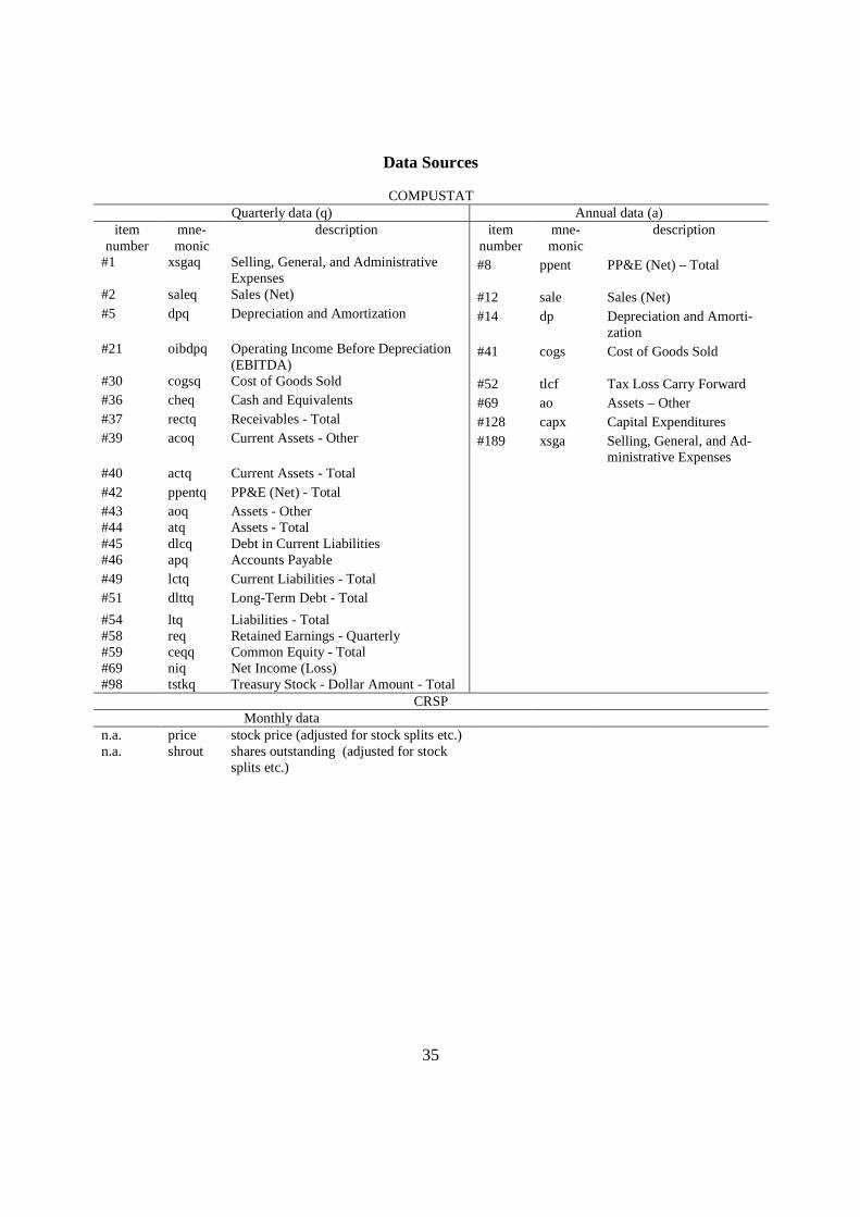
35

Data Sources

COMPUSTAT Quarterly data (q) Annual data (a)

item number

mne-monic

description item number

mne-monic

description

#1 xsgaq Selling, General, and Administrative Expenses

#8 ppent PP&E (Net) – Total

#2 saleq Sales (Net) #12 sale Sales (Net) #5 dpq Depreciation and Amortization #14 dp Depreciation and Amorti-

zation #21 oibdpq Operating Income Before Depreciation

(EBITDA) #41 cogs Cost of Goods Sold

#30 cogsq Cost of Goods Sold #52 tlcf Tax Loss Carry Forward #36 cheq Cash and Equivalents #69 ao Assets – Other #37 rectq Receivables - Total #128 capx Capital Expenditures #39 acoq Current Assets - Other #189 xsga Selling, General, and Ad-

ministrative Expenses #40 actq Current Assets - Total #42 ppentq PP&E (Net) - Total #43 aoq Assets - Other #44 atq Assets - Total #45 dlcq Debt in Current Liabilities #46 apq Accounts Payable #49 lctq Current Liabilities - Total

#51 dlttq Long-Term Debt - Total #54 ltq Liabilities - Total #58 req Retained Earnings - Quarterly #59 ceqq Common Equity - Total #69 niq Net Income (Loss) #98 tstkq Treasury Stock - Dollar Amount - Total

CRSP Monthly data

n.a. price stock price (adjusted for stock splits etc.) n.a. shrout shares outstanding (adjusted for stock

splits etc.)

36

Table 1: Sample selection procedure

Description Time Period

Observations (Firm Quarters)

No. of firms (Compustat identifier: GVKEY)

1 Firm-quarter observa-tions on the intersection of COMPUSTAT and CRSP

1961Q1-2009Q4 940,513 22,904

2 drop observations with changing fiscal years or duplicates in terms of NPERMNO (unique identifier from the CRSP database) and date or GVKEY (unique identifier from the COMPUSTAT database) and date

1961Q1-2009Q4 -13,726

=926,787

22,904

3 drop observations with missing market data from CRSP

1961Q4-2009Q4 -20,100

=906,687

22,894

4 drop observations that are not within the ex-tended Bhojraj/Lee (2002) SIC code defini-tion

1961Q4-2009Q4 -751,686 =155,001

5,276

5 drop observations, where relevant items* are negative

1971Q1-2009Q4 - 63,223 =91,778

3,779

6 keep data within time span

1992Q1-2009Q4 -19,410 =72,368

3,363

7 drop observations with missing data for the Schwartz-Moon input parameter

1992Q1-2009Q4 -42,891 =29,477

2,262

This table shows the sample selection procedure. We use the quarterly CRSP/Compustat merged database in order to obtain our sample. Thus, all accounting items are from the quarterly Compustat database, with few exceptions such as loss carry forwards which are only available on a yearly basis. These yearly data items are obtained from the Compustat Annual data files. All market data, i.e., prices and shares outstanding, were ob-tained from the monthly CRSP database. Market data from CRSP is used four month after the fiscal year quar-ter for each company to ensure, that market prices incorporate the last available accounting information. We use the high technology industry SIC code definition of Bhojraj and Lee (2002) in this study. That is biotechnology SIC codes (2833-2836 and 8731-8734), computer SIC Codes (3570-3577 and 7371-7379), electronics (3600-3674) and telecommunication (4810-4841) extended in this paper by SIC code 7370. The considered time span ranges from Q1 1992 to Q4 2009. * These items -stated as Compustat mnemonics- are: acoq aoq apq capxy cheq cogsq tlcf dlcq dlttq dpq ppentq rectq saleq tstkq xsgaq.

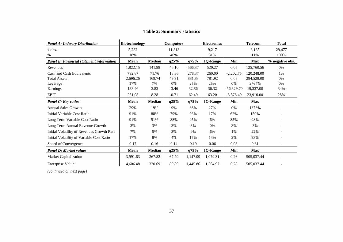
37

Table 2: Summary statistics

Panel A: Industry Distribution Biotechnology Computers Electronics Telecom Total

# obs. 5,282 11,813 9,217 3,165 29,477 % 18% 40% 31% 11% 100%

Panel B: Financial statement information Mean Median q25% q75% IQ-Range Min Max % negative obs.

Revenues 1,822.15 141.98 46.10 566.37 520.27 0.05 125,760.56 0%

Cash and Cash Equivalents 792.87 71.76 18.36 278.37 260.00 -2,202.75 120,248.00 1% Total Assets 2,696.26 169.74 49.91 831.83 781.92 0.68 284,528.00 0% Leverage 17% 7% 0% 25% 25% 0% 2764% 0% Earnings 133.46 3.83 -3.46 32.86 36.32 -56,329.70 19,337.00 34%

EBIT 261.08 8.28 -0.71 62.49 63.20 -5,378.40 23,910.00 28%

Panel C: Key ratios Mean Median q25% q75% IQ-Range Min Max

Annual Sales Growth 29% 19% 9% 36% 27% 0% 1373% -

Initial Variable Cost Ratio 91% 88% 79% 96% 17% 62% 150% -

Long Term Variable Cost Ratio 91% 91% 88% 95% 6% 85% 98% -

Long Term Annual Revenue Growth 3% 3% 3% 3% 0% 3% 3% -

Initial Volatility of Revenues Growth Rate 7% 5% 3% 9% 6% 1% 22% -

Initial Volatility of Variable Cost Ratio 17% 8% 4% 17% 13% 2% 93% -

Speed of Convergence 0.17 0.16 0.14 0.19 0.06 0.08 0.31 -

Panel D: Market values Mean Median q25% q75% IQ-Range Min Max

Market Capitalization 3,991.63 267.82 67.79 1,147.09 1,079.31 0.26 505,037.44 -

Enterprise Value 4,606.48 320.69 80.89 1,445.86 1,364.97 0.28 505,037.44 -

(continued on next page)

38

(Table 2 continued)

This table reports summary statistics for a sample of 29,477 technology firm quarter observations. Panel A reports the sample's industry distribution accord-ing to Bhojraj and Lee (2002) with SIC codes in parentheses: biotechnology (2833-2836 and 8731-8734), computers (3570-3577 and 7370-7379), electron-ics (3600-3674) and telecommunications (4810-4841). Note that we add SIC code 7370 to their sample definition. Panel B reports financial statement in-formation. All financial statement items are on a quarterly basis (q) unless stated otherwise as annual items (a) in appendix 1. Note that quarterly flow fig-ures are aggregated to meaningful yearly figures. Thus, each observation contains the sum of the last four quarter values. COMPUSTAT item mnemonics are given in parenthesis. All values are given in million $ except of percentages denoted as %. Revenues are given by sales (saleq). Cash and cash equiva-lents is calculated as the sum of cash (cheq), receivables total (rectq), current assets other (acoq) and treasury stocks (tstkq) minus accounts payable (apq). Total assets is the balance sheet total (atq). Leverage is calculated as interest bearing debt, which is the sum of debt in current liabilities (dlcq) and long term debt (dlttq), divided by total assets (atq). Earnings are defined as net income/loss (niq) and EBIT is operating income (oibdpq) after depreciation (dpq). Panel C reports key ratios. Annual sales growth is the annualized growth rate of the current quarter. The initial variable cost ratio is measured by the mean of the ratio of costs of goods sold (cogsq) plus selling, general, and administrative expenses (xsgaq) divided by sales (saleq). Long term variable cost ratio is calculated using a growing window approach based on three digit SIC code industry classification beginning in 1970 and until the most recent quarter. The long term annual growth rate of revenues is set to 3%. The initial volatility of revenue growth rates is determined from the standard deviation of the residu-als from an AR(1) regression of the growth rates. Analogously, the initial volatility of the variable cost ratio is determined from the AR(1) regression resid-uals of the cost ratios. The speed of convergence parameters result from the convergence of the previous eight quarterly sales data points as presented in appendix 1. Panel D reports market data. Market capitalization is calculated from CRSP as price times shares outstanding. Enterprise value is the sum of market capitalization, long term debt (dlttq) and debt in current liabilities (dlcq).

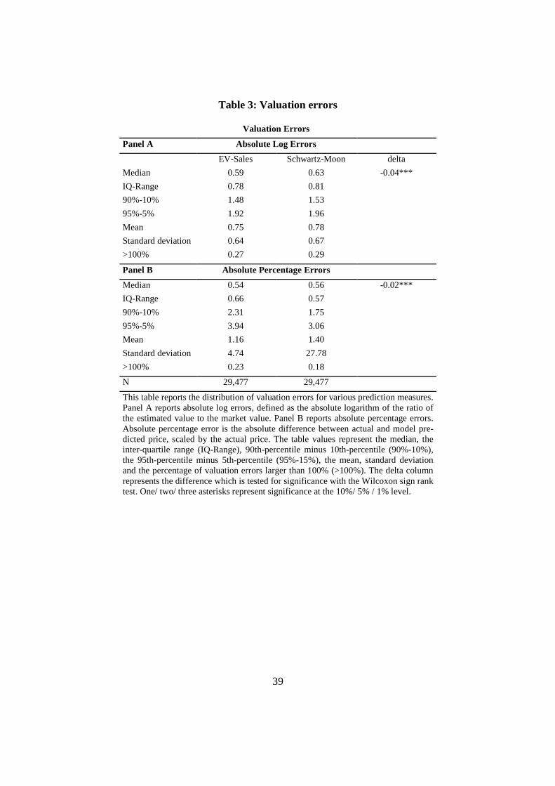
39

Table 3: Valuation errors

Valuation Errors

Panel A Absolute Log Errors

EV-Sales Schwartz-Moon delta

Median 0.59 0.63 -0.04***

IQ-Range 0.78 0.81

90%-10% 1.48 1.53

95%-5% 1.92 1.96

Mean 0.75 0.78

Standard deviation 0.64 0.67

>100% 0.27 0.29

Panel B Absolute Percentage Errors

Median 0.54 0.56 -0.02***

IQ-Range 0.66 0.57

90%-10% 2.31 1.75

95%-5% 3.94 3.06

Mean 1.16 1.40

Standard deviation 4.74 27.78

>100% 0.23 0.18

N 29,477 29,477

This table reports the distribution of valuation errors for various prediction measures. Panel A reports absolute log errors, defined as the absolute logarithm of the ratio of the estimated value to the market value. Panel B reports absolute percentage errors. Absolute percentage error is the absolute difference between actual and model pre-dicted price, scaled by the actual price. The table values represent the median, the inter-quartile range (IQ-Range), 90th-percentile minus 10th-percentile (90%-10%), the 95th-percentile minus 5th-percentile (95%-15%), the mean, standard deviation and the percentage of valuation errors larger than 100% (>100%). The delta column represents the difference which is tested for significance with the Wilcoxon sign rank test. One/ two/ three asterisks represent significance at the 10%/ 5% / 1% level.

40

Table 4: Valuation errors by industry classification and firm size

Median Absolute Log Errors

Panel A: by 2 digit SIC codes

Industry EV-Sales Schwartz-Moon delta # obs.

28 chemicals 0.62 0.52 0.11*** 3,799

35 computer (hardware) 0.65 0.53 0.11*** 3,272

36 electronics 0.56 0.57 -0.01* 9,217

48 telecommunication 0.47 1.00 -0.53*** 3,165

73 computer (software) 0.61 0.59 0.02*** 8,541

87 biological research 0.70 1.49 -0.80*** 1,483

Total 0.59 0.63 -0.04*** 29,477

Panel B: by firm size classification 0 - 25% 0.72 0.70 0.03** 7,370

26% - 50% 0.62 0.61 0.01* 7,369

51% -75 % 0.54 0.56 -0.02* 7,369

76% - 100% 0.50 0.64 -0.15*** 7,369

Total 0.59 0.63 -0.04*** 29,477

This table reports the distribution of median log valuation errors, defined as the absolute logarithm of the ratio of the estimated value to the market value for firms. Panel A reports absolute log errors for firms according to their two digit SIC code. Panel B reports absolute log errors by firm size quartile. Firm size is measured by total assets (Compustat item: atq). The delta column represents the difference which is tested for significance with the Wilcoxon sign rank test. One/ two/ three asterisks represent significance at the 10%/ 5% / 1% level.

41

Table 5: Trading Strategy

Panel A: Abnormal Returns before Transaction Costs

12 months 24 months 36 months

fixed

long monthly abn. Ret

1.19%

1.05%

0.92%

t-statistic

(2.34)*** (2.05)**

(1.82)*

short

monthly abn. Ret

0.46%

0.40%

0.42%

t-statistic

(0.79) (0.70)

(0.76)

quin

tiles

long monthly abn. Ret

1.16%

1.07%

0.92%

t-statistic

(2.27)** (2.12)**

(1.83)*

short

monthly abn. Ret

0.36%

0.39%

0.42%

t-statistic

(0.60) (0.68)

(0.74)

Panel B: Abnormal Returns after Transaction Costs

12 months 24 months 36 months

fixed

long monthly abn. Ret

1.03%

0.98%

0.88%

t-statistic

(2.04)** (1.92)*

(1.74)*

short monthly abn. Ret

0.34%

0.34%

0.39%

t-statistic

(0.59) (0.61)

(0.70)

quin

tiles

long monthly abn. Ret

0.99%

1.00%

0.88%

t-statistic

(1.94)* (1.99)**

(1.75)*

short

monthly abn. Ret

0.24%

0.34%

0.39%

t-statistic

(0.41) (0.59)

(0.68)

This table presents the results for a long (short) trading strategy for undervalued (overvalued) stocks

identified by the Schwartz-Moon model. Every quarter stocks enter the portfolio for a predefined time span of 1, 2 and 3 years due to the Schwartz-Moon model. The "fixed" column represents a trading strategy based on an over- or undervaluation of more than 50%. For the "quintiles" column the stocks are sorted into quintiles every quarter according to the misvaluation predicted by the Schwartz-Moon model. The most undervalued (overvalued) quintile is then invested in (sold short). The portfolios assume a 1$ investment in every stock and stocks can enter the portfolio multiple times. For these portfolios Panel A shows the intercept in basis points from a regression of the monthly portfolio ex-cess return on the four factors of Carhart (1997) for the period 1992 to 2009 (N=216). Further, it shows the t-statistics of these intercepts and the t-statistic of the difference of the portfolio returns. The "short" portfolios assume short positions, thus trading profits are represented by positive alphas. Panel B displays the abnormal returns after transaction costs by using the results of Keim and Madhaven (1998). We use heteroskedasticity-robust standard errors. One/ two/ three asterisks represent signifi-cance at the 10%/ 5% / 1% level.

42

Table 6: Model implied default probability

Default rates Schwartz-Moon Median 29% Mean 35% Standard deviation 29% Zero default obs. 492 All default obs. 256

This table reports summary statistics of model implied default rates for 29,477 firm quarter observations for the Schwartz-Moon model. Median, mean, and standard deviation values are obtained by the ratio between defaulted simulation paths and 10,000, the total number of simulations per firm quarter. Zero/All de-fault obs. reports observations in which the respective model predicted no/complete fail-ure in all simulation paths.

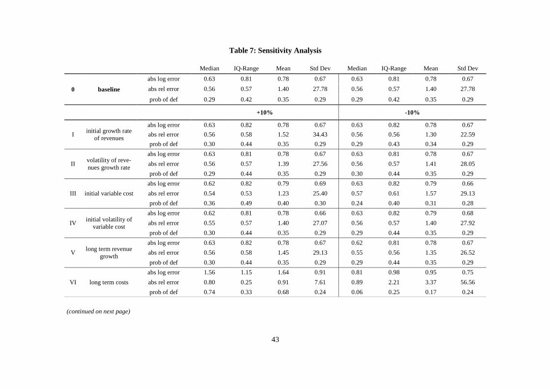
43

Table 7: Sensitivity Analysis

Median IQ-Range Mean Std Dev Median IQ-Range Mean Std Dev

0 baseline

abs log error 0.63 0.81 0.78 0.67 0.63 0.81 0.78 0.67

abs rel error 0.56 0.57 1.40 27.78 0.56 0.57 1.40 27.78

prob of def 0.29 0.42 0.35 0.29 0.29 0.42 0.35 0.29

+10% -10%

I initial growth rate

of revenues

abs log error 0.63 0.82 0.78 0.67 0.63 0.82 0.78 0.67

abs rel error 0.56 0.58 1.52 34.43 0.56 0.56 1.30 22.59

prob of def 0.30 0.44 0.35 0.29 0.29 0.43 0.34 0.29

II volatility of reve-nues growth rate

abs log error 0.63 0.81 0.78 0.67 0.63 0.81 0.78 0.67

abs rel error 0.56 0.57 1.39 27.56 0.56 0.57 1.41 28.05

prob of def 0.29 0.44 0.35 0.29 0.30 0.44 0.35 0.29

III initial variable cost

abs log error 0.62 0.82 0.79 0.69 0.63 0.82 0.79 0.66

abs rel error 0.54 0.53 1.23 25.40 0.57 0.61 1.57 29.13

prob of def 0.36 0.49 0.40 0.30 0.24 0.40 0.31 0.28

IV initial volatility of

variable cost

abs log error 0.62 0.81 0.78 0.66 0.63 0.82 0.79 0.68

abs rel error 0.55 0.57 1.40 27.07 0.56 0.57 1.40 27.92

prob of def 0.30 0.44 0.35 0.29 0.29 0.44 0.35 0.29

V long term revenue

growth

abs log error 0.63 0.82 0.78 0.67 0.62 0.81 0.78 0.67

abs rel error 0.56 0.58 1.45 29.13 0.55 0.56 1.35 26.52

prob of def 0.30 0.44 0.35 0.29 0.29 0.44 0.35 0.29

VI long term costs

abs log error 1.56 1.15 1.64 0.91 0.81 0.98 0.95 0.75

abs rel error 0.80 0.25 0.91 7.61 0.89 2.21 3.37 56.56

prob of def 0.74 0.33 0.68 0.24 0.06 0.25 0.17 0.24

(continued on next page)

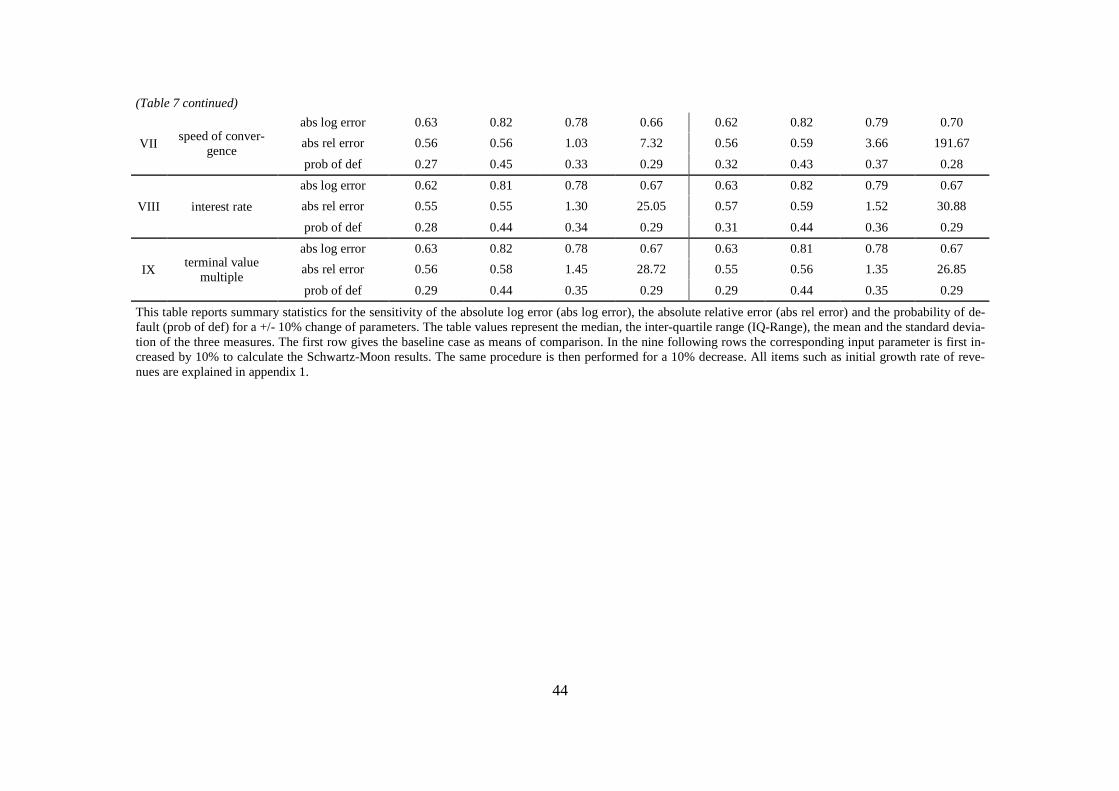
44

(Table 7 continued)

VII speed of conver-

gence

abs log error 0.63 0.82 0.78 0.66 0.62 0.82 0.79 0.70

abs rel error 0.56 0.56 1.03 7.32 0.56 0.59 3.66 191.67

prob of def 0.27 0.45 0.33 0.29 0.32 0.43 0.37 0.28

VIII interest rate

abs log error 0.62 0.81 0.78 0.67 0.63 0.82 0.79 0.67

abs rel error 0.55 0.55 1.30 25.05 0.57 0.59 1.52 30.88

prob of def 0.28 0.44 0.34 0.29 0.31 0.44 0.36 0.29

IX terminal value

multiple

abs log error 0.63 0.82 0.78 0.67 0.63 0.81 0.78 0.67

abs rel error 0.56 0.58 1.45 28.72 0.55 0.56 1.35 26.85

prob of def 0.29 0.44 0.35 0.29 0.29 0.44 0.35 0.29

This table reports summary statistics for the sensitivity of the absolute log error (abs log error), the absolute relative error (abs rel error) and the probability of de-fault (prob of def) for a +/- 10% change of parameters. The table values represent the median, the inter-quartile range (IQ-Range), the mean and the standard devia-tion of the three measures. The first row gives the baseline case as means of comparison. In the nine following rows the corresponding input parameter is first in-creased by 10% to calculate the Schwartz-Moon results. The same procedure is then performed for a 10% decrease. All items such as initial growth rate of reve-nues are explained in appendix 1.

45

Table 8: Regression Analysis

Industry/Size Type Coeffi-cient

Constant No. of obs.

Overall R² (fixed effects)/

Adj. R² (rank regression)

Prob. > F

Panel A

28 chemicals Fixed Effects 0.12*** 21.66*** 3,799 0.18 0.00

Rank Regression 0.90*** 388.93*** 3,799 0.83 0.00

35 computer

(hardware) Fixed Effects 0.13*** 16.33*** 3,272 0.38 0.00

Rank Regression 0.93*** 21.02*** 3,272 0.86 0.00

36 electronics Fixed Effects 0.19*** 15.85*** 9,217 0.45 0.00

Rank Regression 0.96*** -1222.46** 9,217 0.84 0.00

48 telecommunica-

tion Fixed Effects 0.10*** 39.01*** 3,165 0.30 0.00

Rank Regression 0.77*** 6058.77*** 3,165 0.74 0.00

73 computer (software)

Fixed Effects 0.08*** 16.63*** 8,541 0.16 0.00

Rank Regression 0.92*** 1800.03*** 8,541 0.80 0.00

87 biological research

Fixed Effects 0.12*** 19.67*** 1,483 0.17 0.01

Rank Regression 0.79*** 6486.30*** 1,483 0.66 0.00

all Fixed Effects 0.13*** 20.02*** 29,477 0.32 0.00

Rank Regression 0.89*** 1676.00*** 29,477 0.79 0.00

Panel B

0 - 25% Fixed Effects 0.04*** 6.40*** 7,370 0.07 0.00

Rank Regression 0.40*** 2835.11*** 7,370 0.15 0.00

26% - 50% Fixed Effects 0.04*** 13.40*** 7,369 0.05 0.00

Rank Regression 0.30*** 7712.83*** 7,369 0.09 0.00

51 - 75% Fixed Effects 0.09*** 23.14*** 7,369 0.12 0.00

Rank Regression 0.42*** 10363.46*** 7,369 0.20 0.00

76% - 100% Fixed Effects 0.14*** 39.12*** 7,369 0.33 0.00

Rank Regression 0.54*** 11680.79*** 7,369 0.34 0.00

all Fixed Effects 0.13*** 20.02*** 29,477 0.32 0.00

Rank Regression 0.89*** 1676.00*** 29,477 0.79 0.00 This table reports the results of a fixed effects regression and a rank regression of observed firm value on predicted firm value including a constant. We choose the fixed effects specification after rejecting the random effects model based on a Hausman test (p<0.01). In addition, the fixed effects model is also preferred to a pooled OLS estimate after performing an F-test on the firm fixed effects, which are significantly different from zero. The fixed effects regressions are performed on a per share basis and take time and firm cluster effects into account as in Petersen (2009). Adjusted R2 is reported for the rank regression, while the overall R2 shows model fit in case of the fixed effect estimates. The rank OLS regressions are performed on market values consistent with Iman and Conover (1979). Panel A presents regressions which are performed per two digit SIC industry classification. Panel B shows the results per size quartile, which is measured by total assets. One/ two/ three asterisks represent significance at a 10%/ 5%/ 1% level.

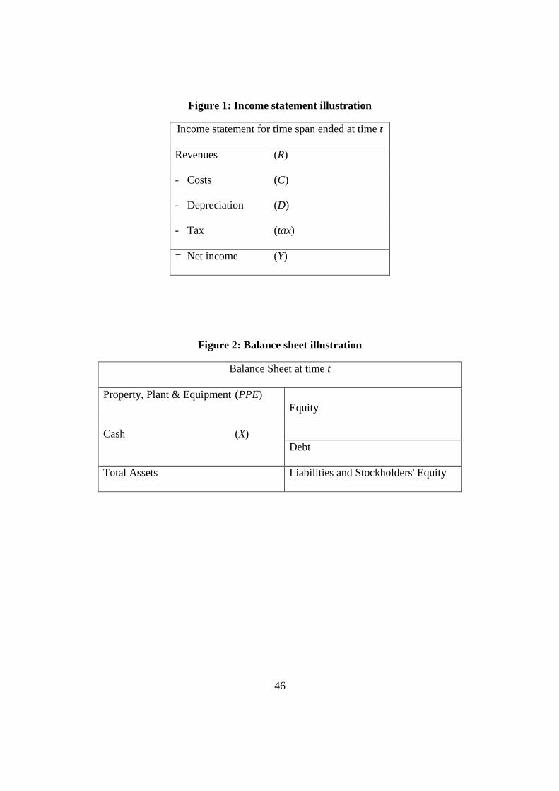
46

Figure 1: Income statement illustration

Income statement for time span ended at time t

Revenues (R)

- Costs (C)

- Depreciation (D)

- Tax (tax)

= Net income (Y)

Figure 2: Balance sheet illustration

Balance Sheet at time t

Property, Plant & Equipment (PPE) Equity

Cash (X) Debt

Total Assets Liabilities and Stockholders' Equity

47

Figure 3: Valuation error distribution Panel A: Kernel-density plot of log valuation errors

Panel B: Kernel-density plot of relative valuation errors

0.1

.2.3

.4.5

dens

ity

-5 0 5log error

EV-SalesSchwartz-Moon

0.2

.4.6

.8

dens

ity

-2 0 2 4 6relative error

EV-SalesSchwartz-Moon

This figure shows a kernel density plot of valuation errors for the two different valuation approaches on a sample of 29,477 technology firm quarter observations. Panel A reports log valuation errors defined as the logarithm of the ratio of the estimated value to the market value. Panel B reports relative valuation errors which is the difference between actual and model predicted value, scaled by the actual value. The blue, solid line reports valuation errors for the Enterprise-Value-Sales-Multiple. The red, dashed line reports valuation errors for the Schwartz-Moon model.

48

Figure 4: Quarterly median absolute valuation errors Panel A: Quarterly absolute log errors

Panel B: Quarterly absolute percentage errors

010

0020

0030

0040

00

Nas

daq

.5.6

.7.8

.9ab

s. lo

g. v

alua

tion

erro

r

1992q1 1996q3 2001q1 2005q3 2010q1quartal

EV-SalesSchwartz-MoonNasdaq

010

0020

0030

0040

00

Nas

daq

.4.5

.6.7

.8.9

abs.

rel

. val

uatio

n er

ror

1992q1 1996q3 2001q1 2005q3 2010q1quartal

EV-SalesSchwartz-MoonNasdaq

This figure shows quarterly median valuation errors spanning the time 1992 until 2009. Panel A reports median absolute log errors defined as the absolute logarithm of the ratio of the estimated value to the mar-ket value. Panel B reports median absolute relative valuation errors which is the absolute difference be-tween actual and model predicted value, scaled by the actual value. The blue, solid line reports valuation errors for the Enterprise-Value-Sales-Multiple. The red, dashed line reports valuation errors for the Schwartz-Moon model. The green, dashed-dotted line reports the Nasdaq Composite as benchmark.

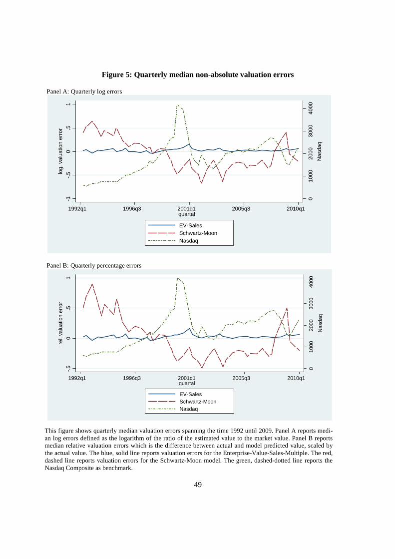
49

Figure 5: Quarterly median non-absolute valuation errors Panel A: Quarterly log errors

Panel B: Quarterly percentage errors

010

0020

0030

0040

00

Nas

daq

-1-.

50

.51

log.

val

uatio

n er

ror

1992q1 1996q3 2001q1 2005q3 2010q1quartal

EV-SalesSchwartz-MoonNasdaq

010

0020

0030

0040

00

Nas

daq

-.5

0.5

1

rel.

valu

atio

n er

ror

1992q1 1996q3 2001q1 2005q3 2010q1quartal

EV-SalesSchwartz-MoonNasdaq

This figure shows quarterly median valuation errors spanning the time 1992 until 2009. Panel A reports medi-an log errors defined as the logarithm of the ratio of the estimated value to the market value. Panel B reports median relative valuation errors which is the difference between actual and model predicted value, scaled by the actual value. The blue, solid line reports valuation errors for the Enterprise-Value-Sales-Multiple. The red, dashed line reports valuation errors for the Schwartz-Moon model. The green, dashed-dotted line reports the Nasdaq Composite as benchmark.

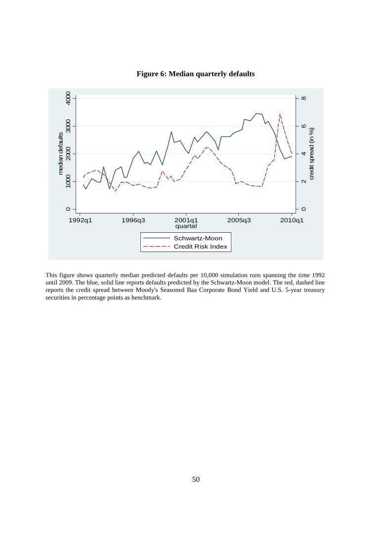
50

Figure 6: Median quarterly defaults

02

46

8cr

edit

spre

ad (in

%)

010

00200

030

0040

00m

edia

n de

faults

1992q1 1996q3 2001q1 2005q3 2010q1quartal

Schwartz-MoonCredit Risk Index

This figure shows quarterly median predicted defaults per 10,000 simulation runs spanning the time 1992 until 2009. The blue, solid line reports defaults predicted by the Schwartz-Moon model. The red, dashed line reports the credit spread between Moody's Seasoned Baa Corporate Bond Yield and U.S. 5-year treasury securities in percentage points as benchmark.