Valuing guaranteed minimum death benefits in

variable annuities and the option to lapse∗

Blessing Mudavanhu†

Walter A. Haas School of BusinessUniversity of California, Berkeley

Berkeley, CA 94720 USAmudavanh@haas.berkeley.edu

Jun Zhuo

American International Group, Inc.Market Risk Management70 Pine Street, 20th Floor

New York, NY 10270 USAjun.zhuo@aig.com

March 2002

Abstract

Many variable annuities provide money-back guarantees and market guarantees on investedprincipal. Embedded in some of these guarantees are stochastic maturity put options withadjustable strike prices. These variable annuities can be surrendered or lapsed at any time.The lapse option when exercised rationally represents an American style sell-back option thatis exercised by the policyholder when the embedded put option is out-of-the-money. The deathbenefits we consider are only exercised involuntary, that is, upon the death of the policyholder.Critical to the valuation analysis is that the embedded put options have stochastic maturity andthat the policyholder can exercise the lapse, or early-exercise, option feature to increase the valueof the contract and thereby exposing the insurance company to loss of fees. We analyze specificvariable annuity products by focusing on the lapse option when exercised either rationally orirrationally, taking into account the mortality risk and surrender charges.

Keywords and phrases: American option, lapse option, lookback option, stochastic maturity∗Submitted to the North American Acturial Journal for publication.†The research reported in this paper was started while the first author was at American International Group

(AIG), Inc. He wishes to acknowledge AIG’s Market Risk Management Division for financial support.

1

1 Introduction

The variable annuity (VA) market has shown tremendous growth in the past decade. This has

largely been driven by demographic factors - i.e. the aging baby boomers and the demand for

retirement savings - and the simultaneous performance of strong U.S. equity markets.

However, the risk-return profile of the VA business is highly correlated with the future evolution

of U.S. equity markets. This is true for two reasons. First, the size of the lucrative asset-based fees

is dependent on a strong equity market. Second, the guaranteed minimum death benefit (GMDB)

- which is a ubiquitous component of every contract - exposes annuity writers to claims during

prolonged periods of weak equity markets. As such, their business model is doubly exposed to

equity market risks. Indeed, faced with an aggregate $1 trillion VA market - and after coming

to grips with the potential magnitude of the GMDB risk - the reinsurance markets for GMDBs

has virtually dried up. The few remaining players do not provide the wide range of features and

capacities needed to efficiently reinsure the books of some of the largest annuity writers. At the

same time, the reinsurance rate for GMDB risk also increased significantly.

Therefore, the only feasible alternative to managing the potentially hazardous risks embedded in

VA policies is for a large annuity writer to undertake a self reinsurance plan using traded capital

market instruments.

To this end, the first step is to value the GMDBs in variable annuities in the same framework

that capital markets use to value derivatives. In fact, there have been studies (cf. Milevsky and

Posner (2001), Grosen and Jorgensen (1977 & 1999) and references therein) on computing the no

arbitrage value of GMDBs using the well-established derivative pricing models. The methodology

traces its roots to the famous Black-Scholes option pricing formula, and has become the standard

valuation technique for traded capital market instruments. The main contribution from this work

is that we value the GMDBs and the option to lapse in an actual variable annuity contract and

take into account the surrender charges schedule. Our results give annuity writers more realistic

indications on the costs of GMDBs in their products. In this paper, we value guaranteed minimum

death benefit (GMDB) options in Polaris1 II variable annuities.1Polaris II VAs are provided by SunAmerica Inc., a subsidiary of American International Group, Inc.

2

2 Product description

There are two types of guaranteed minimum death benefit (GMDB) options in Polaris II VA. These

are: the purchase payment accumulation (PPA) option and maximum anniversary value (MAV)

option. The PPA option provides interest rate guarantees as well as market guarantees. The basic

PPA option guarantees a return of at least the original invested premium at time zero compounded

at a 4% annual growth rate until the date of death (3% growth rate if 70 or older at the time of

contract issue). Technically, the payout to the beneficiary is: max(egτV0, Vτ ), g is the guaranteed

instantaneous growth rate, V0 is the invested principal and Vτ is the value of the investment at the

time of death. The time of death is treated as a stochastic random variable.

The MAV option provides a money-back guarantee (without a growth rate) as well as market guar-

antees. The basic MAV option is based on a suitably defined highest anniversary account value.

Technically, under the MAV option, the payout to the beneficiary is max(Vτ , M∗τ ) where M∗

τ is

the maximum of anniversary value of the contract prior to the policyholders’ 81st birthday. If the

policyholder is 90 or older at the time of death, the death benefit will be equal to the value of the

contract at the time of death. In option pricing theory the guarantee corresponds to having a strike

price of the embedded option that floats and may increase to a new higher level every year. The

floating piece is determined on the anniversary market value of the contract. A detailed description

of the PPA and MAV options is provided in Appendix A.

The term interest guarantee refers to a GMDB where the original premium is guaranteed to accu-

mulate at a fixed rate of return (for example, the PPA option). The term market guarantee refers

to a GMDB where some degree of market returns are guaranteed in the form of anniversary resets

(for example, the MAV option).

Our goal is to compute the fair values of GMDB options in Polaris II VA which are essentially

derivatives that remain alive as long as the policyholder does not die or lapse. Rational investors

will lapse the option when the embedded put options are out-of-the-money. However, the insur-

ance company provides a disincentive for policyholders to leave the fund by imposing lapsation or

surrender charges. Surrender charges secure sunk commissions costs, and the insurance company

is also protecting itself by increasing the probability of receiving fees that are meant to pay for the

death benefit option. GMDB options with a lapse option exercised rationally have an American

style feature otherwise they exhibit European style features. (By European style features, we refer

to options that are only exercised at maturity. Early exercisable options are said to exhibit Amer-

ican style features.) Unlike standard financial options, the embedded options in VA are not paid

3

for upfront, instead they are paid for as an insurance charge deducted from the underlying fund

periodically. Formal valuation methods for these GMDB options are complicated by the fact that

the underlying options exhibit American-style sell-back features and they have stochastic maturity.

The options are exercised involuntary since they are only triggered by death. Stochastic maturity,

where the maturity is independent of the underlying asset, is eccentric to classical option pricing

theory and as such it has not been dealt with sufficiently. There are some exotic stochastic matu-

rity options, such as barrier options, where the maturity depends on the underlying asset. To the

extent that the payoff structure of the death benefit options in many variable annuities are between

European and American style and are triggered by death, Milevsky and Posner (cf. Milvesky and

Posner (2000)) have labeled these options Titanic options. Related work on stochastic maturity op-

tions was studied by Carr (1998) for financial instruments he called randomized American options.

While GMDB options are not freely traded between policyholders and capital markets participants,

the assumption of perfect markets guides us to a relative value. In our study, we do not consider

credit risk, that is, default on the side of the fund manager.

The organization of this report is as follows; we will begin by considering simplified versions of the

two GMDBs in the Polaris II VA. Then, we will study the lapsation option which is the main focus

of this paper. For the special cases of the product, we provide closed-form analytical solutions

and the more general cases are handled by an American Monte Carlo method for the illustrative

examples. We also study perpetual options to provide upper bounds for present values of MAV and

PPA options. Throughout this paper, the final payoff at the date of death of the policyholder or

when he/she exercises the lapse option, is assumed to be based on an initial premium of 100 units

at time zero. We finish this paper with some concluding remarks.

4

3 The model

We will use the following nomenclature;

Dτ ¤ death payment at time τPE ¤ GMDB (without lapsation) option payoffPA ¤ GMDB (with lapsation) option payoffVt ¤ market value of the investment at time t (years)V ∗

k ¤ market value of the investment at the kth anniversary dateM∗

τ ¤ maximum anniversary value of the investment at death.τ ¤ stochastic death time of the policyholderT ¤ deterministic death time of the policyholderg ¤ guaranteed growth rate

αt ¤ lapsation (or surrender) charge at time tδ ¤ insurance charge and management feesr ¤ risk-free interest rateσ ¤ volatility

The maturity date refers to the termination of the accumulation phase which we may assume, for

simplicity, to be set2 at the inception of the contract. Superscripts p and m will be used to denote

the PPA and the MAV death benefit options respectively.

The progression of the fund value, which we treat as a single asset is modeled as

dVt = (µ− δ)Vtdt + σVtdWt (1)

where Wt is a standard Brownian motion, µ is the drift rate and δ is a sum of management fees

and insurance charges (also called mortality and expense (M&E) fees) that pays for the underlying

option. This reflects that, unlike standard financial options, the embedded options in VA are not

paid for upfront, instead they are paid for as insurance charge deducted from the underlying fund

on a periodic basis. The insurance charge and the management fees are modeled as a dividend

yield outflow3 δ, since this dividend does not go to the fund-holder but to the insurance company.

Thus, a continuous time payment δVt flows to the insurer. In the examples that follow, we choose

δ = 2% and δ = 2.5% which are consistent with the insurance charges and management asset fees

in Polaris II VA.

The risk neutral process for Vt follows the lognormal process;

dVt = (r − δ)Vtdt + σVtdWQt (2)

2In the Polaris II VA, the investor determines when the income phase begins.3We distinguish these from actual dividends on the underlying assets which are assumed to be automatically

reinvested in the fund.

5

where r is a risk-free rate, and dWt is a Brownian motion under a new Girsanov-transformed

measure Q. The stochastic differential equation (2) has a well known solution given by

Vt = V0e(r−δ−σ2/2)t+σW Q

t . (3)

In the following sections, we will consider different aspects of PPA and MAV death benefit options.

3.1 Simulations

We use a hybrid of Monte Carlo simulation procedures and tree methods. The Monte Carlo tech-

nique works by building simulated paths for the underlying security price which are computed

recursively. Under the geometric Brownian motion assumption, the price paths are generated by

solving equation (2) thus,

Vi∆t = V(i−1)∆te(r−δ−σ2/2)∆t+σ

√∆tzi , i = 1, 2, · · · , n (4)

where ∆t is the length of the time interval between two successive prices and the zi are random

numbers drawn from a standard Gaussian distribution. The Monte Carlo simulation and generic

tree building procedures we use are implemented in NumeriX Time Libraries provided by Nu-

meriX, LLC (2000). The method used is similar to the stochastic mesh method (cf. Broadie and

Glasserman (2000)).

3.2 Mortality

We shall use standard 1994 VA MGDB mortality data shown in Figure 1. The data shows the

conditional death probability p(x + i; 1) for a male (and p(x + i; 1), for a female) aged x + i to die

prior to age x + i + 1 for i = 0, 1, 2, · · · . For simplicity and convenience, future lifetime random

variables can be expressed in continuous time by extrapolating a probability distribution function

from the mortality table (cf. Milevsky and Posner (2000)).

4 Interest guarantee option

One of the death benefit options in the Polaris II VA is a Purchase Payment Accumulation (PPA)

option. The PPA death benefit option is the greater of: the value of the contract at the time of

death; or the invested premium compounded at a 4% annual growth rate until the date of death

(3% growth rate if 70 or older at the time of contract issue); or the value of the contract on the

6

0 5 10 15 20 25 30 35 40 45 500

0.5

1

1.5

2

2.5

3

3.5x 10

−3

cond

ition

al d

eath

pro

babi

lity

age

male mortality female mortality

50 55 60 65 70 75 80 85 90 95 100

0.05

0.1

0.15

0.2

0.25

0.3

0.35

0.4

age

cond

ition

al d

eath

pro

babi

lity

Figure 1: 1994 VA MGDB mortality data.

seventh anniversary compounded at a 4% annual growth rate until the date of death (3% growth

rate if 70 or older at the time of contract issue). We can think of this option as a reset death benefit

option since, as shown below, it has an embedded put option with a strike price reset option at

the seventh anniversary date. However, we will call the death benefit options interest guarantee

options because of the guranteed growth rate specified in the contract. The fund payoff of a contract

containing a PPA death benefit option can be described as follows:

DpT =

(1− αt)Vt, for all t, if lapsedmax(egτV0, VT ), t ≤ 7, at death (t = τ)max(egτV0, e

g(τ−7)V ∗7 , Vτ ), t > 7, at death (t = τ)

(5)

where αtVt is the amount of the surrender charge at time t (in years). In Polaris II VA, one of the

surrender charges (which we will use here) is a piecewise step (ratchet-down) function defined as

αt ={

8%− 1%× ceil(t), t ≤ 70, t > 7

(6)

where ceil(·) rounds the arguments to the nearest intergers towards infinity.

7

4.1 PPA option with deterministic lifetime and no lapsation

If we further assume that the policyholder dies before the seventh anniversary of the contract and

does not annuitize early, the fund payout is simply the death payment

DpT = max(egT V0, VT ) (7)

which can conveniently be rewritten as

DpT = egT max(V0 − e−gT VT , 0) + VT . (8)

Thus,

DpT = egT PE(T, V0; g) + VT (9)

(cf. Grosen and Jorgensen (1997)). We note that egT PE(T, V0; g) is a weighted European put

option whose strike price is the initial value of the policy V0 with an underlying asset Vt discounted

by the guaranteed growth rate g. Alternatively, the exercise price of the put option increases at a

rate g. Therefore, the present value Dp0 of the total claim that the investor has on the insurance

company at time zero can be represented as

Dp0 = EQ

{e−rT Dp

T

}= EQ

{e−(r−g)T max(V0 − e−gT VT , 0) + e−rT VT

}(10)

where EQ{·} is an expectation. Due to arbitrage considerations 0 < g < r at the inception of the

contract. Making the classical assumption that Vt follows a geometric Brownian motion (2) and

noting that

EQ{e−rT VT

}= e−δT V0 (11)

since

VT = V0e(r−δ− 1

2σ2)T+σW

we obtain a Black-Scholes type solution,

Dp0 = V0

[BS(r, δ, σ, T ) + e−δT

]≡ V0([e−brTN(−d2)− e−δTN(−d1)] + e−δT ) (12)

where

d1 =(r − δ + σ2/2)

√T

σ, d2 = d1 − σ

√T and r = r − g. (13)

N(·) is the cumulative probability function for a random variable that is standard normally dis-

tributed. Notice that the guaranteed growth rate lowers the discounting factor, thereby increasing

the value of the GMDB option, thus the embedded put option price increases at the rate of g. If

8

0 5 10 15 20 25 30 35 40 45 50100

105

110

115

120

pres

ent v

alue

contract lifetime (years)

δ =0

growth rate =0 growth rate=3% growth rate =4%

0 5 10 15 20 25 30 35 40 45 5020

40

60

80

100

120

pres

ent v

alue

contract lifetime (years)

δ =2.5%

growth rate =0 growth rate=3% growth rate =4%

Figure 2: A comparison of a European style PPA option (without a 7th year anniversary reset) andcontract lifetime for σ = 20% and r = 6%.

g = 0 we will call the option, one that only guarantees the invested principal, a plain vanilla GMDB

option4. Thus a plain vanilla death benefit option has the payoff

DT = max(V0, VT ) (14)

and its present value is given by (12). The plain vanilla death benefit option guarantees a limited

loss of (1 − e−rT )V0 due to the time value of money. Figure 2 shows a comparison of the present

value of a European style PPA option (without a 7th year anniversary reset) with contract lifetime.

The dividend payout δ represents payments charged to the account. These payments implicitly

reduce the value of the fund under management. We note that the embedded put options actually

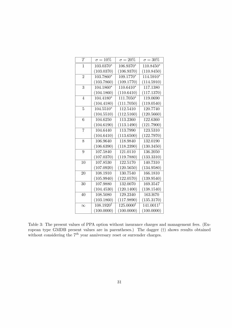
increase in value with increasing dividends. In Appendix C, Table 3 shows (for g = 4% and T = 3)

that the value of the put option with δ = 0 is 4.1860 (= 104.1860 − 100) and in Table 4 (for

δ = 2.5%) the value increases to 7.1776 (= 99.9519− e−0.025×3100).

Now, if we assume that the policyholder dies after the seventh anniversary, the payoff of the death4The plain vanilla GMDB option defined here is not provided in Polaris II VA, but it is an artifact we use for

comparison.

9

benefit option is

DpT = max(egT V0, e

g(T−7)V ∗7 , VT ). (15)

This death benefit option can be rewritten as

DpT =

{max(eg(T−7)V ∗

7 , VT ), V0 < e−g7V ∗7

max(egT V0, VT ), V0 ≥ e−g7V ∗7 .

(16)

We derive a closed form solution for the present value of the option which has a reset guarantee by

making the classical assumption that, in the risk neutral world, Vt follows the geometric Brownian

motion (2). In the interest of brevity we take δ = g = 0, otherwise the general derivation follows

from the steps below. Therefore, we consider

DpT = VT +

{max(V ∗

7 − VT , 0), V0 < V ∗7

max(V0 − VT , 0), V0 ≥ V ∗7

. (17)

Based on the risk neutral valuation, the value at inception of the death benefit contract is given by

Dp0 = V0

[N(a2(7))

[e−br(T−7)N(−a2(T − 7))− e−δ(T−7)N(−a1(T − 7))

](18)

+ e−brTN2(−a2(7),−a2(T ),√

7/T )−N2(−a1(7),−a1(T ),√

7/T ) + e−δT]

where

a1(x) =(r − δ + σ2/2)

√x

σ, a2(x) = a1(x)− σ

√x and r = r − g.

N2(·) stands for the standard bivariate normal cumulative probability distribution function. Refer

to the derivation in Appendix B. If T ≤ 7, the explicit formula (18) for the death benefit reset option

reduces to the explicit formula (12) for the death benefit without a reset option. Figure 3 shows

a comparison of European style plain vanilla death benefit option values with the corresponding

PPA and MAV options. The impact of the seventh anniversary reset option on the present value of

the PPA option is large compared to the plain vanilla death benefit option. The exponential decay

of the option value is due to the insurance charge and management fees. The low present values

of the death benefit options suggests that for large T (i.e., young investors), policyholders over-pay

for the embedded put options if they do not exercise the lapse option.

Example: Consider a contract with an initial value equal to 100 units of the account, that is,

V0 = 100 and calculate the fair value of a European style PPA option. The contract is assumed

to be subject to the following market and deal parameters; r = 6%, σ = 10%, 20% or 30% and

δ = 0% or δ = 2.5%. Tables 3 and 4 in Appendix C show a summary of the results (written in

parentheses). The results are very close to exact values obtained using the explicit solution (12)

if the policyholder dies before the 7th anniversary. For uniformity, simulation results rather than

exact values are tabulated here, even for cases where closed form solutions exist, since other features

of the GMDBs discussed below do not have closed form solutions.2

10

0 5 10 15 20 25 30 35 40 45 5020

30

40

50

60

70

80

90

100

110

contract lifetime (years)

GM

DB

pre

sent

val

ue

MAV GMDB PPA GMDB Plain vanilla GMDB

Figure 3: Present value of European style GMDB option for σ = 20% and r = 6%.

4.2 Lapse option and surrender charges

The GMDB in Polaris II VA also gives the policyholder an American style option (if the lapse

option is exercised rationally) to cash out the contract from the issuing company anytime he/she

likes. This feature is known in the insurance business as a surrender option. We will call this option

a lapsation option. Rational investors will lapse the contract when the embedded put options are

out-of-the-money. Lapsation will be thought of as rational if: i) it is immediately followed by a

reestablishment of a contract with a better guarantee, i.e., one that has an embedded option with

a higher strike price, or ii) the contract policy value minus surrender charges is greater than the

present value of the death benefit option. In the first case, the option to lapse is really an option to

raise the strike price of the embedded put option when it out-of-the-money even after the lapsation

charges are applied. We will focus on the second case where we do not worry about what the

policyholder does with the payoff. Clearly the option to lapse raises the value of death benefit

options and as such increases the exposure of the issuing company to the loss of fees. The death

benefit payout at death time τ is given by

Dpτ = PA(τ, V0, V

∗7 ; g) + Vτ (19)

11

The American style put option in (19) is computed by using the American Monte Carlo method.

We warn readers that due to the nonlinearity of the early exercise features, equation (19) cannot

be solved separably (as is the case with the European style version), instead we will solve (19) as a

non-separable death benefit option. In order for a cohort of policyholders to remain invested in the

contract and fully pay for the embedded put options they are provided with, the insurance company

charges for surrendering the option. Thus, the death benefit is meant to be lapse supported. The

value of the death benefit depends on how rational policyholders choose to lapse in a bear or bull

market. If policyholders panic, they will lapse and the company will not issue embedded GMDB

option payments but it will loose fees. By definition, the insurance contract shares cost among

individuals in an underwriting class.

Example Revisited Tables 3 and 4 in Appendix C show a summary of results obtained based

on a step-down surrender charge function when the reset GMDB option is valued considering the

lapse option. The asterisk (∗) indicates that it is not optimal to lapse the death benefit option.2

4.3 PPA option with a stochastic lifetime

When the maturity date τ is stochastic and independent of Vt, the present value of the GMDB is

given by an expectation with respect to both Vt and τ . The death benefit option present value is

given by

Dp0 = Ex

{EQ

{e−rτDp

τ | τ = t}}

. (20)

The first expectation is taken over the random maturity while the second is taken over the future

asset price at a given realization of the random maturity. The present value of the stochastic

maturity European put option is then given by

Dp0 = V0[

∫ K

0fx(t)BS(r, σ, t)dt + 1] (21)

where K is the maximum term of the contract and fx(t) is the probability density function of the

future lifetime random variable. Equation (21) establishes a relationship between random and fixed

maturity GMDBs (cf. Milevsky and Posner (2001)). Parametric mortality functions may also be

used. For a given issue age, a higher value of K increases the probability that the policyholder will

die and use the embedded put option.

Alternatively, the lifetime variable can also be incorporated into a binomial tree valuation scheme by

assuming a time-dependent probability of death at each node. Thus, the value at each node equals

the value of the contract if the policyholder does not die times his/her survival probability plus

12

the value if he/she dies times his/her probability of dying. Using conditional probabilities of dying

provided in the 1994 VA MGDB mortality table, shown in Figure 1, and the deterministic maturity

death benefit option values, we obtain American style GMDB present values with a stochastic

maturity given by

Dp0 =

105−x∑

j=1

q(x; j)Dp0(j) (22)

for a male aged x at the inception of the contract, where Dp0(j) is the present value (with an early

exercise option) of a GMDB with maturity j. The quantity q(x; j) denotes the probability that

a male aged x will rationally surrender or involuntary exercise the death benefit option in the jth

year. This probability is defined by

q(x; j) =j−2∏

i=0

(1− p(x + i; 1)) · p(x + j − 1; 1) (23)

for all j = 2, 3, · · · , and

q(x; 1) = p(x; 1).

We note that105−x∑

j=1

q(x; j) = 1, (24)

assuming that policyholders do not live beyond 105 years. Surrender charges are automatically

incorporated into the valuation scheme. Similarly, for a female aged x, we substitute p and q in

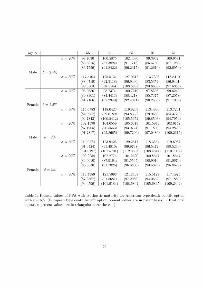
the above formulas with p and q corresponding to female conditional death probabilities. Table 1

below summarises the results for for different sexes and ages of policyholders.

13

4.4 Irrational lapsation

Assuming that there is a 5% irrational lapsation rate denoted by l, an investor aged x will lapse

the contract in the first year with probability l or die with probability p(x; 1). (Lapsation statistics

on variable annuities shows that between 5% and 8% of the policyholders exercise the lapse option

every year.) Thus, the probability of non-optimally (or irrationally) surrendering the GMDB option

or exercising it (involuntary) in the first year is ql(x; 1) = p(x; 1) + l. In general, the probability

that a male aged x will irrationally surrender or exercise the GMDB option in the jth year is given

by

ql(x; j) =j−2∏

i=0

(1− p(x + i; 1)− l) · (p(x + j − 1; 1) + l) (25)

for j = 2, 3, · · · , and

ql(x; 1) = p(x; 1) + l.

Thus, the GMDB present value of a male aged x assuming an annual lapsation rate of l = 5% is

given by

Dp0 =

105−x∑

j=2

ql(x; j)p(x + j − 1; 1) + l

[p(x + j − 1; 1)Dp

0(j) + l∗j−1e−δ(j−1)V0

](26)

and

Dp0 = p(x; 1)Dp

0(1) + e−δl∗0V0

where

l∗j = l · (1−max(7− j, 0)%) (27)

has been adjusted for surrender charges in the first seven years and Dp0(j) is the present value of

a European style death benefit option with maturity j. Similar results directly follow for female

policyholders. Unlike in (22), the surrender charges in equation (27) are incorporated in ql(x + j)

and not implemented in the valuation schemes since Dp0(j) assumes that investors die in the jth year

and have no early exercise feature. Table 1 shows a summary of results 〈in triangular parenthesis〉considering irrational lapsation.

4.5 Perpetual plain vanilla death benefit option

The PPA option we have discussed can be generalized as providing the payoff,

DT = PA + VT (28)

14

at time T , where PA is an American style put option that has deterministic maturity T with

an appropriate strike price. It is well known that PA → 0 as T → ∞ (i.e., the put option

becomes worthless with increasing time to maturity). Considering dividend payouts, the value

of the underlying asset VT → 0 as T → ∞ , since EQ{VT } = e−δT V0. Therefore DT → 0, which

implies that European style death benefit options are not valuable for young investors.

15

5 Market guarantee option

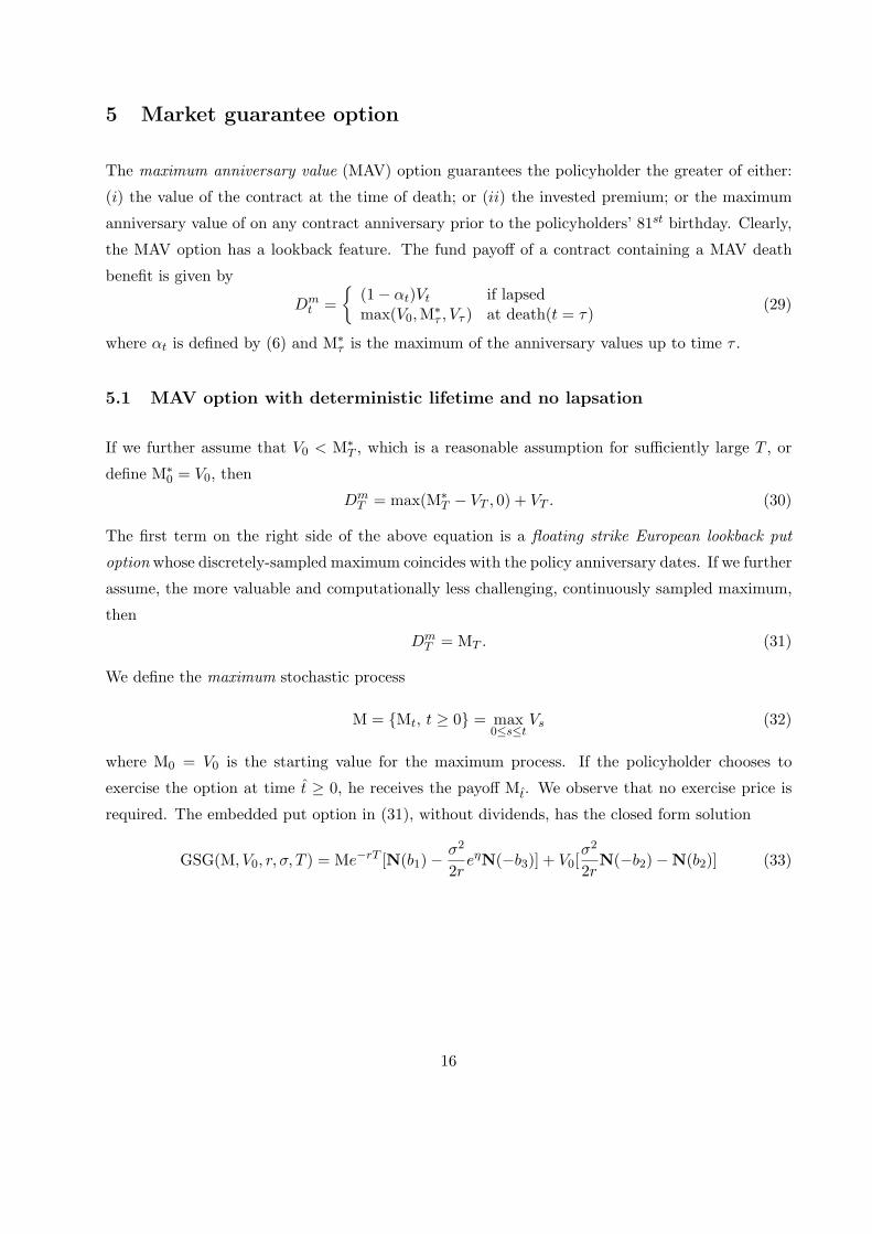
The maximum anniversary value (MAV) option guarantees the policyholder the greater of either:

(i) the value of the contract at the time of death; or (ii) the invested premium; or the maximum

anniversary value of on any contract anniversary prior to the policyholders’ 81st birthday. Clearly,

the MAV option has a lookback feature. The fund payoff of a contract containing a MAV death

benefit is given by

Dmt =

{(1− αt)Vt if lapsedmax(V0, M∗

τ , Vτ ) at death(t = τ)(29)

where αt is defined by (6) and M∗τ is the maximum of the anniversary values up to time τ .

5.1 MAV option with deterministic lifetime and no lapsation

If we further assume that V0 < M∗T , which is a reasonable assumption for sufficiently large T , or

define M∗0 = V0, then

DmT = max(M∗

T − VT , 0) + VT . (30)

The first term on the right side of the above equation is a floating strike European lookback put

option whose discretely-sampled maximum coincides with the policy anniversary dates. If we further

assume, the more valuable and computationally less challenging, continuously sampled maximum,

then

DmT = MT . (31)

We define the maximum stochastic process

M = {Mt, t ≥ 0} = max0≤s≤t

Vs (32)

where M0 = V0 is the starting value for the maximum process. If the policyholder chooses to

exercise the option at time t ≥ 0, he receives the payoff Mt. We observe that no exercise price is

required. The embedded put option in (31), without dividends, has the closed form solution

GSG(M, V0, r, σ, T ) = Me−rT [N(b1)− σ2

2reηN(−b3)] + V0[

σ2

2rN(−b2)−N(b2)] (33)

16

where

b1 =ln(M/V0)− (r − σ2/2)T

σ√

T

b2 = b1 − σ√

T

b3 =ln(M/V0) + (r − σ2/2)T

σ√

T

η =2(r − σ2/2) ln(M/V0)

σ2

and M is the maximum investment value achieved to date (cf. Goldman, Sosin and Gatto (1979)).

As for the MAV death benefit option, under the continuously sampled maximum assumption, we

obtain the present value of the death benefit option as

Dm0 = GSG(M, V0, r, σ, T ) + V0 (34)

where δ = 0. The present value of the death benefit option payoff for the more practical discretely-

sampled maximum can be approximated by simulation and tree methods or by continuous adjust-

ments of the discretely-sampled maximum (cf. Broadie et al (1998)).

Example Revisited: Tables 5 and 6 in Appendix B show a summary of European style MAV

present values (shown in parentheses) considering step-down surrender charges. The asterisk (∗)indicates that it is not optimal to lapse the GMDB option.2

5.2 Lapse option and surrender charges

Example Revisited: Tables 5 and 6 in Appendix B show a summary of a American style MAV

present values considering step-down surrender charges. The asterisk (∗) indicates that it is not

optimal to lapse the GMDB option.2

Figure 4 shows a comparison of American style GMDBs. The present values approach a limit of

approximately 93 for increasing contract years. This limit is related to surrender charges.

5.3 MAV option with a stochastic lifetime

When τ is stochastic and independent of Vt, the present value of the death benefit option is given

by an expectation with respect to both Vt and τ . The death benefit option present value is given

by

Dp0 = Ex

{EQ

{e−rτDp

τ | τ = t}}

17

0 5 10 15 20 25 30 35 40 45 5092

94

96

98

100

102

104

106

108

contract lifetime (years)

GM

DB

pre

sent

val

ue

Plain Vanilla GDMBMAV GMDB PPA GMDB

Figure 4: The American style death benefit option with insurance charges and management feesfor σ = 20%, δ = 2.5% and r = 6%.

18

The present value of the stochastic maturity European type MAV option, with continuously sampled

maximum, is then given by

Dm0 =

∫ K

0fx(t)[GSG(M, V0, r, σ, t) + V0]dt (35)

where K is the maximum term of the contract and fx(t) is the probability density function of the

future lifetime random variable. Using the mortality data shown in Figure 1 and already computed

MAV options with deterministic maturity, we obtain present values for different sexes and ages

shown in Table 2 below. We assume that the policyholder annuitizes at their 90th birthday since

after that the MAV option does not have a death benefit option.

19

5.4 Perpetual MAV option

The perpetual American style MAV option is related to a Russian option which at any time chosen

by the holder as the stopping time, pays out the maximum (defined by equation (32)) realised asset

price M up to that date. Thus, the Russian option value provides an upper bound for the value of

the perpetual MAV option. When the dividend yield is zero, it is never optimal to hold a Russian

option. If the holder of the option chooses to exercise the option at τ∗ ≥ 0, he/she receives the

payoff M∗τ . The fair price for the Russian option, which provides an upper bound for the perpetual

MAV, is given by

D0 =V0

γ1 − γ2[γ2α

γ1 − γ1αγ2 ] (36)

where

α =(

γ2(γ1 − 1)γ1(γ2 − 1)

) 1γ2−γ1

(37)

and

γ1,2 =12− r − δ

σ2∓

√(12− r − δ

σ2

)2

+2r

σ2(38)

with γ1 < 0 < 1 < γ2, and the optimal stopping time t∗ is the first time t for which

t∗ = inf{t ≥ 0 : αVt ≤ Mt} (39)

(cf. Basso and Pianca (2001)).

The present values of perpetual MAV option, assuming continuously sampled maximum, are sum-

marized in Table 6. Clearly the results show that continuous sampling makes the MAV option very

valuable. When the dividend yield is zero i.e., δ = 0, it is clearly never optimal to lapse the MAV

option.

6 Concluding remarks

In this paper we have proposed a methodology for pricing GMDBs using the well-developed capital

markets valuation framework by taking into account mortality risk, lapse option and surrender

charges. The mortality risk is implemented discretely using the 1994 VA GMDB mortality data.

Our results indicate that the lapse option significantly increases the GMDB option value. Both

death benefit options are much more valuable for middle aged to senior investors compared to

younger investors because of M&E fees. Younger investors are less likely going to die (and exercise

the embedded option) when the GMDBs are most valuable. Our results show that the Polaris II VAs

20

are very sensitive to M&E charges. The valuation strategy we have presented could be used to value

many insurance products such as equity-linked life insurance policies (ELLIPs) with interests rate

guarantees, guaranteed investment contracts (GICs), guaranteed minimum accumulation benefits

(GMABs) and guaranteed minimum income benefits (GIMBs). The valuation strategy can also be

used to influence insurance product design.

Further research will expand on the methodology outlined in this paper to deal with more complex

realistic market parameters such as stochastic interest rate and volatility. Complex lapsation issues

also need to be addressed. Finally, alternative hedging strategies for the death benefits will be

investigated.

Acknowledgements

This study was supported by the Market Risk Management department at American International

Group (AIG), Inc. The authors thank Chuck Lucas, Joe Koltisko, Victor Masch and Mark Rubin-

stein for their advice and suggestions.

21

References

[1] Basso, A. and Pianca, P. “Correcting simulation bias in discrete monitoring of Russian op-

tions.” Working Paper, 2001.

[2] Broadie, M., Glasserman, P. and Kou, S. “A continuity correction for discrete barrier options,”

Mathematical Finance, 7: 325-349, 1997.

[3] Broadie, M., Glasserman, P. and Kou, S. “Connecting discrete and continuous path-dependent

options”, Finance and Stochastics, 3: 55-82, 1999.

[4] Broadie, M. and Glasserman, P., “A stochastic mesh method for pricing high-dimensional

American options”.

[5] Carr, P. “Randomization and the American put.” The Review of Financial Studies, 11 (3):

597-626, 1998.

[6] Cox, J. C., Ross, S. A., and Rubinstein, M. “Option pricing: A simplified approach.” Journal

of Financial Economics, 7: 229-263, 1979.

[7] Goldman, M. B., Sosin, H. B., and Gatto, M. A. “Path-dependent options: buy at the low,

sell at the high”. Journal of Finance, 39: 1511-1524, 1984.

[8] Grosen, A. and Jorgensen, P. L. “Valuation of early exercisable interest rate guarantees.” The

Journal of Risk and Insurance, 64 (3): 481-503, 1997.

[9] Grosen, A. and Jorgensen, P. L. “Fair valuation of life insurance liabilities: The impact of

interest rate guarantees, surrender options, and bonus policies.” Working paper, April 1999.

[10] Haug, E. P. The Complete Guide to Option Pricing Formulas. McGraw Hill, New York, 1998.

[11] Hull, J. C. Options, Futures and Other Derivatives. Prentice Hall, Englewood Cliffs, 4th edition,

1999.

[12] Karatzas, I. and Shreve, S. Methods of Mathematical Finance, Springer Verlag, New York,

1998.

[13] Karatzas, I. and Shreve, S. E. Brownian Motion and Stochastic Calculus. Springer Verlag, New

York, 1988.

[14] Lai, T. L. and Lim, T. W. “Exercise regions and efficient valuation of American lookback

options.” Working Paper, 2001.

22

[15] Milevsky M. and Posner S. “The Titanic Option: Valuation of the guaranteed minimum death

benefit in variable annuities and mutual funds.” The Journal of Risk and Insurance, to appear

2000.

[16] Rubinstein, M. and Reiner, E. “Breaking down the barriers”. Risk, 28-35, September 1991.

[17] Wilmott, P. Derivatives: The Theory and Practice of Financial Engineering. Wiley, New York,

1998.

[18] Zhang, P. G. Exotic Options: A Guide to Second Generation Options, 2nd edition. World

Scientific, Singapore, 1998.

23

Appendix A: Product Description

(a) Purchase Payment Accumulation Option (PPA) Option:

The death benefit is the greater of:

1. the value of the contract at the time the policyholders’ death; or

2. total payment less any withdrawals (and any fees or charges applicable to such withdrawals),

compound at a 4% annual growth rate until the date of the policyholders’ death (3% growth

rate if 70 or older at the time of contract issue plus any Purchase Payment less withdrawals

recorded after the policyholders’ death (and any fees and charges applicable to such with-

drawals); or

3. the value of the contract on the seventh contract anniversary, plus any Purchase Payments

and less any withdrawals (and any fees or charges applicable to such withdrawals), since the

seventh contract anniversary, all compounded at a 4% annual growth rate until the time of

policyholders’ death (3% growth rate if 70 or older at the time of contract issue) plus any

Purchase Payments less withdrawals recorded after the date of death (and any fees or charges

applicable to such withdrawals).

(b) Maximum Anniversary Value (MAV) Option:

The death benefit is the greater of:

1. the value of the contract at the time the policyholders’ death; or

2. total payment less any withdrawals (and any fees or charges applicable to such withdrawals);

or

3. the maximum anniversary value on any contract anniversary prior to policyholders’ 81st

birthday. The anniversary value equals the value of the contract on its anniversary plus any

Purchase Payments and less any withdrawals (and any fees or charges applicable to such

withdrawals), since that anniversary.

If the policyholder is aged 90 or older at the time of death, the MAV death benefit option will be

equal to value of the contract at the time of the policyholders’ death. Accordingly, the policyholders

do not get the advantage of the MAV option if:

24

• they are over age 80 at the time of contract issue, or

• they are aged 90 or older at the time of their death.

Fees and charges:

1. An annual insurance charge of 1.52% applies for the value of contract invested in Variable

Portfolios.

2. A withdrawal charges applies against each Purchase Payment put into the contract. The

withdrawal charge percentage declines (by a percentage point) each year a Purchase Payment

is in the contract. After a Purchase Payment has been in the contract for 7 complete years

(or 9 years if the policyholder elects to participate in the Principal Rewards Program) no

withdrawal charge applies.

3. A maintenance fee is subtracted from the policyholders’ account once per year. A $35 contract

maintenance fee ($30 in North Dakota) from the policyholders’ account value on the contract

anniversary. If the policyholder withdraws their entire contract value, a maintenance fee is

deducted from that withdrawal. If the contract value is $50,000 or more on the contract

anniversary date, the charge will be waived.

25

Appendix B: Derivation of the PPA Solution

Based on the risk neutral valuation, the value at inception of the death benefit contract is given

by;

Dp0 = e−rTEQ

{Dp

T

}

= e−rTEQ {(V ∗7 − VT )IA}+ e−rTEQ {(V0 − VT )IB}+ e−rTEQ {VT }

≡ DpA0 + DpB

0 + V0 (40)

where DpT is given by (), I(·) is an indicator function and A and B are the events;

A ⇔ {V ∗7 > V0 ; VT < V ∗

7 }

and

B ⇔ {V ∗7 ≤ V0 ; VT < V0} .

The first expectation can easily be calculated by observing that given the value of the death benefit

option at the seventh anniversary V ∗7 , the expected value of the option when the event A occurs at

the seventh anniversary is given by

DpA7 = e−r(T−7)EQ {max (V ∗

7 − VT , 0)}= V ∗

7

[e−r(T−7)N(−d2(T − 7))−N(−d1(T − 7))

](41)

where

d1(x) =(r + σ2/2)

√x

σand d2(x) = d1(x)− σ

√x.

Since DpA7 is independent of V ∗

7 , we compute the final expectation for the event A by multiplying

by the probability Pr(V0 < V ∗7 ) which implies

Pr(V0 < V0eµ7+σW7) = Pr(−σW7 < µ7) = N(d2(7)) (42)

where µ = r − σ2/2. Therefore,

DpA0 = e−r7EQ {N(d2(7))DpA

7 }= V0 N(d2(7))

[N(d1(T − 7))− e−r(T−7)N(d2(T − 7))

](43)

since e−r7EQ{V ∗7 } = V0. For the event B, we have

EQ {IB} = Pr(V ∗7 ≤ V0 , VT < V0)

= Pr(V0eµ7+σW7 ≤ V0 , V0e

µT+σWT < V0). (44)

26

Thus,

Pr(σW7 ≤ −µ7 , σWT < −µT ) = N2(−d2(7),−d2(T ),√

7/T ) (45)

where N2(·) stands for the standard bivariate normal cumulative probability distribution function,

N2(ξ, η, ρ) ≡ 12π(1− ρ2)

∫ ξ

−∞

∫ η

−∞e−x2+y2−2ρxy

2(1−ρ2) dxdy (46)

where ρ is the correlation coefficient. So,

EQ {VTIB} = EQ{V0e

µT+σWT IB

}(47)

We define Q by settingdQdQ

= eσWT− 12σ2T (48)

Girsanov’s theorem implies that Wt = Wt − σt follows a standard Brownian motion under the

probability measure Q, therefore,

erTEQ{

eσWT− 12σ2TIB

}≡ erTEQ {IB} . (49)

Following the previous steps, we obtain

EQ{

V0eµ7+σcW7+σ27 ≤ V0 ; V0e

µT+σcWT +σ2T < V0

}

= N2(−d1(7),−d1(T ),√

7/T ) (50)

Thus,

DpB0 = e−rTEQ {(V0 − VT )IB} (51)

= V0[e−rTN2(−d2(7),−d2(T ),√

7/T )−N2(−d1(7),−d1(T ),√

7/T )].

Finally, putting all the above results together, we obtain the present value of the seventh anniversary

reset death benefit option

Dp0 = V0

[N(d2(7))

[e−r(T−7)N(−d2(T − 7))−N(−d1(T − 7))

](52)

+ e−rTN2(−d2(7),−d2(T ),√

7/T )−N2(−d1(7),−d1(T ),√

7/T ) + 1].

Similarly, with dividend payments and a growth rate, we obtain

Dp0 = V0

[N(a2(7))

[e−br(T−7)N(−a2(T − 7))− e−δ(T−7)N(−a1(T − 7))

](53)

+ e−brTN2(−a2(7),−a2(T ),√

7/T )−N2(−a1(7),−a1(T ),√

7/T ) + e−δT]

where

a1(x) =(r − δ + σ2/2)

√x

σand a2(x) = a1(x)− σ

√x.

27

Appendix C: Summary of Results

28

age ¤ 55 60 65 70 75σ = 20% 98.7030 100.5875 102.4030 99.3962 100.9581

〈83.6815〉 〈87.3824〉 〈91.1713〉 〈85.5780〉 〈87.1286〉(86.7559) (91.8422) (96.2315) (91.2610) (92.6950)

Male δ = 2.5%σ = 30% 117.5104 125.5134 127.0612 113.7303 113.8410

〈88.0719〉 〈92.5118〉 〈96.9490〉 〈83.5354〉 〈86.9441〉(99.9563) (104.9284 ) (108.8903) (93.8603) (97.6883)

σ = 20% 96.9686 98.7374 100.7219 97.8598 99.6249〈80.8301〉 〈84.4413〉 〈88.4218〉 〈85.7375〉 〈87.2058〉(81.7166) (87.2940) (92.4041) (90.2503) (91.7956)

Female δ = 2.5%σ = 30% 114.6783 118.0423 119.9269 113.4936 113.7261

〈84.5957〉 〈89.0189〉 〈93.8335〉 〈79.9668〉 〈84.3720〉(94.7843) (100.5412) (105.5652) (89.8503) (94.7959)

σ = 20% 102.1590 104.0559 105.6319 101.5943 102.9152〈87.1905〉 〈90.5553〉 〈93.9724〉 〈91.1800〉 〈94.2820〉(91.2817) (95.8665) (99.7200) (97.0480) (100.2615)

Male δ = 2%σ = 30% 119.9274 123.9425 129.2617 118.3564 119.6957

〈91.0424〉 〈95.4810〉 〈99.9738〉 〈96.5472〉 〈98.5230〉(101.0197) (107.5791) (112.3303) (108.4844) (110.7069)

σ = 20% 100.2258 102.2774 104.2520 100.8547 101.8547〈84.6010〉 〈87.9164〉 〈91.5565〉 〈88.9010〉 〈91.0670〉(86.6530) (91.7826) (96.3800) (93.5823) (95.8629)

Female δ = 2%σ = 30% 113.4389 121.5093 124.8407 115.5179 117.4975

〈87.3867〉 〈91.8681〉 〈97.2086〉 〈94.0552〉 〈97.1880〉(94.0599) (101.9184) (108.6804) (105.6845) (109.2304)

Table 1: Present values of PPA with stochastic maturity for American type death benefit optionwith r = 6%. (European type death benefit option present values are in parentheses.) 〈 Irrationallapsation present values are in triangular parentheses. 〉

29

age ¤ 55 60 65 70 75σ = 20% 94.3208 95.1073 96.1560 97.5618 100.4126

〈80.2057〉 〈83.7263〉 〈87.5147〉 〈91.4164〉 〈95.3998〉(75.2928) (81.7271) (87.8268) (93.2336) (97.8262)

Male δ = 2.5%σ = 30% 105.2010 107.8749 110.0316 112.7163 114.2086

〈86.1462〉 〈90.6629〉 〈95.3435〉 〈99.9007〉 〈104.2567〉(93.2848) (99.4495) (105.0306) (109.3480) (112.4550)

σ = 20% 93.8251 94.3420 95.0534 96.1521 98.9025〈77.5434〉 〈80.7965〉 〈84.5693〉 〈88.8374〉 〈93.5456〉(70.1107) (76.7889) (83.5855) (90.0170) (95.7427)

Female δ = 2.5%σ = 30% 101.9377 106.2933 108.0558 111.6858 113.7806

〈82.6483〉 〈86.9690〉 〈91.8770〉 〈97.1318〉 〈102.6067〉(88.1776) (94.8304) (101.5862) (107.2200) (111.6295)

σ = 20% 95.1989 96.3358 98.6930 100.5343 102.7832〈84.2647〉 〈87.4466〉 〈90.8334〉 〈94.2846〉 〈97.7485〉(81.8253) (87.3982) (92.6051) (97.1222) (100.8019)

Male δ = 2%σ = 30% 110.9807 112.7460 115.5282 117.1695 117.6693

〈90.4765〉 〈94.6336〉 〈98.8918〉 〈102.9621〉 〈106.7489〉(100.8718) (105.9145) (110.4263) (113.6741) (115.7018)

σ = 20% 94.4344 95.2884 98.2280 99.9031 102.4440〈81.8626〉 〈84.8421〉 〈88.2684〉 〈92.1039〉 〈96.2493〉(77.3077) (83.1610) (89.0671) (94.5423) (99.2105)

Female δ = 2%σ = 30% 109.3570 110.5135 114.4235 116.9644 117.5102

〈87.2536〉 〈91.2829〉 〈95.8380〉 〈100.6296〉 〈105.4854〉(96.6330) (102.1421) (107.8274) (112.2999) (115.4369)

Table 2: The present values of MAV with a stochastic maturity for American type death benefitoption for r = 6%. (European type death benefit option present values are in parentheses.)〈 Irrational lapsation present values are in triangular parentheses. 〉

30

T σ = 10% σ = 20% σ = 30%1 103.0370∗ 106.9370∗ 110.8450∗

(103.0370) (106.9370) (110.8450)2 103.7860∗ 109.1770∗ 114.5910∗

(103.7860) (109.1770) (114.5910)3 104.1860∗ 110.6410∗ 117.1380

(104.1860) (110.6410) (117.1370)4 104.4180∗ 111.7050∗ 119.0690

(104.4180) (111.7050) (119.0540)5 104.5510∗ 112.5410 120.7740

(104.5510) (112.5160) (120.5660)6 104.6250 113.2360 122.6360

(104.6190) (113.1490) (121.7900)7 104.6440 113.7990 123.5310

(104.6410) (113.6500) (122.7970)8 106.9640 118.9840 132.0190

(106.6390) (118.2390) (130.3450)9 107.5840 121.0110 136.2050

(107.0370) (119.7880) (133.3310)10 107.8530 122.5170 140.7310

(107.0920) (120.5650) (134.9580)20 108.1910 130.7540 166.1810

(105.9940) (122.0570) (139.9540)30 107.9880 132.0070 169.3547

(104.4530) (120.1400) (138.1540)40 108.5080 129.2340 163.l670

(103.1860) (117.9890) (135.3170)∞ 108.1920† 125.0000† 141.0011†

(100.0000) (100.0000) (100.0000)

Table 3: The present values of PPA option without insurance charges and management fees. (Eu-ropean type GMDB present values are in parentheses.) The dagger (†) shows results obtainedwithout considering the 7th year anniversary reset or surrender charges.

31

T σ = 10% σ = 20% σ = 30%δ = 2% δ = 2.5% δ = 2% δ = 2.5% δ = 2% δ = 2.5%

1 101.9290∗ 101.6800∗ 105.8290∗ 105.5680∗ 109.7110∗ 109.4400∗

(101.9290) (101.6800) (105.8290) (105.5680) (109.7110) (109.4400)2 101.4960∗ 101.0040∗ 106.8880∗ 106.3630∗ 112.3110 111.6780

(101.4960) (101.0040) (106.8880) (106.3630) (112.2300) (111.6760)3 100.6770∗ 99.9519∗ 107.1330∗ 106.3470∗ 113.5010 112.6660

(100.6770) (99.9519) (107.1330) (106.3470) (113.4980) (112.6610)4 99.6681 98.7270 106.9590 105.9270 114.1310 113.0440

(99.6663) (98.7160) (106.9530) (105.9120) (114.1060) (112.9980)5 98.5905 97.6807 106.6530 105.5750 114.9230 113.7450

(98.5405) (97.3736) (106.5040) (105.2140) (114.2870) (112.8930)6 97.7571 96.8409 106.4150 105.2190 115.4180 114.0260

(97.3397) (95.9650) (105.8680) (104.3340) (114.1670) (112.4990)7 97.1182 96.1457 106.1390 104.8620 115.5340 114.0890

(96.0879) (94.5136) (105.0920) (103.3230) (113.8180) (111.8840)8 96.9510 95.7543 108.3240 106.1190 120.3200 117.8330

(96.3365) (94.4467) (107.6560) (105.4610) (118.9130) (116.4660)9 96.3852 95.1032 109.0250 106.5330 122.7190 119.8200

(95.5157) (93.4236) (107.8540) (105.4120) (120.3410) (117.5560)10 95.7821 94.1032 109.5560 106.8520 125.2730 121.9480

(94.4145) (92.1424) (107.3600) (104.6830) (120.4980) (117.4530)20 93.0628 93.0553 105.4890 101.3460 131.1010 124.0430

(81.7387) (78.2166) (96.9936) (92.6714) (112.3970) (107.2890)30 93.0573 93.0501 98.3791 94.5952 124.1020 115.9490

(69.3919) (65.1646) (84.2423) (78.8493) (97.8854) (92.3701)40 93.0534 93.0478 95.6209 93.1396 112.8765 99.7819

(58.4667) (53.9250) (72.1701) (66.2560) (85.0332) (78.2069)

Table 4: The present values of PPA option with insurance charges and management fees. (Europeantype GMDB present values are in parentheses.)

32

T σ = 10% σ = 20% σ = 30%1 101.6360∗ 105.1670∗ 108.8960∗

(101.6360) (105.1670) (108.8960)2 102.3580∗ 108.1890 114.6200

(102.3580) (108.1710) (114.5640)3 102.8240∗ 110.4920 119.3190

(102.8240) (110.4470) (119.1460)4 103.0580 112.0580 122.6960

(103.0510) (112.0040) (122.5670)5 103.2430 113.4310 125.9760

(103.2310) (113.3220) (125.5850)6 103.2890 114.3680 128.2460

(103.2600) (114.1500) (127.6160)7 103.4820 115.5540 130.8020

(103.4150) (115.1450) (129.7370)8 103.8450 116.6510 133.4200

(103.4050) (115.7830) (131.8400)9 104.1750 117.6050 135.5790

(103.6060) (116.4800) (133.6290)10 103.9690 117.7520 137.5030

(103.4430) (116.5760) (134.4850)20 104.3950 121.762 155.1910

(103.6090) (119.6320) (135.8010)30 104.7450 121.7940 155.5520

(103.6680) (119.5610) (138.0750)40 105.1030 128.3660 207.5310

(103.6140) (120.5730) (144.9700)∞ ∞† ∞† ∞†

(∞†) (∞†) (∞†)

Table 5: The present values of MAV option without insurance charges and management fees.(European type MAV option present values are in parentheses.) The dagger (†) indicates that weare assuming that the strike price of the embedded put option of the GMDB option is reset tomaximum anniversary value every year forever.

33

T σ = 10% σ = 20% σ = 30%δ = 2% δ = 2.5% δ = 2% δ = 2.5% δ = 2% δ = 2.5%

1 100.2320 99.9075∗ 103.6060∗ 103.9060 107.6610 107.3630∗

(100.2320) (99.9075) (103.9060) (103.6060) (107.6610) (107.3630)2 99.4133 98.7399 105.5240 104.8990 111.9890 111.3670

(99.4133) (98.7392) (105.4970) (104.8690) (111.9150) (111.2910)3 98.2553 97.2278 106.3240 105.3680 115.1510 114.1730

(98.2473) (97.2147) (106.2520) (105.2870) (114.9430) (113.9550)4 96.8382 95.4478 106.3490 105.0500 116.9310 115.5940

(96.8278) (95.4312) (106.2740) (104.9720) (116.7100) (115.3570)5 95.3552 93.6467 106.105 104.4770 118.4630 116.7380

(95.2992) (93.5527) (105.9550) (104.3040) (118.0120) (116.2640)6 93.7693 93.0428 105.3570 103.3620 119.0430 116.9490

(93.6275) (91.5228) (105.1060) (103.0960) (118.3540) (116.2570)7 93.0538 93.0451 104.8590 102.5200 119.5050 116.9770

(92.1028) (89.6656) (104.3810) (102.0120) (118.5310) (116.0270)8 93.0561 93.0492 104.3380 101.6680 120.2160 117.2790

(90.3373) (87.5753) (103.4150) (100.7210) (118.7950) (115.9060)9 93.0570 93.0492 103.5110 100.5100 120.4960 117.1980

(88.8244) (85.6925) (102.3440) (99.3252) (118.7150) (115.4550)10 93.0495 93.0431 102.0680 98.8000 120.5410 116.8520

(86.9779) (83.5594) (100.8680) (97.5416) (117.7830) (114.1320)20 93.0624 93.0553 93.8390 93.1502 115.9720 108.3680

(71.7295) (65.7316) (86.9904) (80.7760) (107.1790) (100.0750)30 93.0573 93.0501 93.6297 93.1440 103.5720 97.4791

(58.7546) (51.2586) (71.9736) (63.9861) (91.1920) (81.9129)40 93.0534 93.0473 93.4043 93.1328 112.3250 95.2270

(48.1048) (39.9570) (60.2419) (51.2291) (79.8788) (68.6733)∞ 130.2390† 107.2584† 134.5724† 130.2390† 183.4495† 172.2528†

(00.0000) (00.0000) (00.0000) (00.0000) (00.0000) (00.0000)

Table 6: The present values of MAV option with insurance charges and management fees. (Euro-pean type MAV option present values are in parentheses.) The dagger (†) indicates values computedby assuming continuously sampled maximum without surrender charges.

34