value enhancement: eva, cfroi and other …people.stern.nyu.edu/adamodar/pdfiles/valn2ed/ch32.pdf1...

1

CHAPTER 32

VALUE ENHANCEMENT: EVA, CFROI AND OTHER TOOLS

The traditional discounted cash flow model provides for a rich and thorough

analysis of all the different ways in which a firm can increase value; but it can become

complex, as the number of inputs increases. It is also very difficult to tie management

compensation systems to a discounted cash flow model, since many of the inputs need to

be estimated and can be manipulated to yield the results management wants.

If we assume that markets are efficient, we can replace the unobservable value

from the discounted cash flow model with the observed market price and reward or

punish managers based upon the performance of the stock. Thus, a firm whose stock

price has gone up is viewed as having created value, whereas one whose stock price has

fallen has destroyed value. Compensation systems based upon the stock price, including

stock grants and warrants, have become a standard component of most management

compensation package.

While market prices have the advantage of being up to date and observable, they

are also noisy. Even if markets are efficient, stock prices tend to fluctuate around the true

value and markets sometimes do make mistakes. Thus, a firm may see its stock price go

up and its top management rewarded, even as it destroys value. Conversely, the managers

of a firm may be penalized as its stock price drops, even though the managers may have

taken actions that increase firm value. The other problem with stock prices as the basis

for compensation is that they are available only for the entire firm. Thus, stock prices

cannot be used to analyze the managers of individual divisions of a firm or for their

relative performance.

In the last decade, while firms have become more focused on value creation, they

have remained suspicious of financial markets. While they might understand the notion of

discounted cash flow value, they are unwilling to tie compensation to a value that is based

upon dozens of estimates. In this environment, new mechanisms for measuring value that

are simple to estimate and use, do not depend too heavily on market movements and do

not require a lot of estimation, find a ready market. The two mechanisms that seem to

have made the most impact are:

2

1. Economic Value Added, which measures the dollar surplus value created by a firm

on its existing investment, and

2. Cash Flow Return on Investment, which measured the percentage return made by a

firm on its existing investments

In this chapter, we look at how each is related to discounted cash flow valuation. We also

look at the conditions under which firms using these approaches to judge performance and

evaluate managers may end up making decisions that destroy value rather than create it.

Economic Value Added

The economic value added (EVA) is a measure of the dollar surplus value created

by an investment or a portfolio of investments. It is computed as the product of the

"excess return" made on an investment or investments and the capital invested in that

investment or investments.

Economic Value Added = (Return on Capital Invested – Cost of Capital) (Capital

Invested) = After tax operating income – (Cost of Capital) (Capital Invested)

In this section, we will begin by looking at the measurement of economic value added,

then consider its links to discounted cash flow valuation and close with a discussion of its

limitations as a value enhancement tool.

Calculating EVA

The definition of EVA outlines three basic inputs we need for its computation -

the return on capital earned on investments, the cost of capital for those investments and

the capital invested in them. In measuring each of these, we will make many of the same

adjustments we discussed in the context of discounted cash flow valuation.

How much capital is invested in existing assets? One obvious answer is to use the

market value of the firm, but market value includes capital invested not just in assets in

place but in expected future growth1. Since we want to evaluate the quality of assets in

place, we need a measure of the market value of just these assets. Given the difficulty of

estimating market value of assets in place, it is not surprising that we turn to the book

3

value of capital as a proxy for the market value of capital invested in assets in place. The

book value, however, is a number that reflects not just the accounting choices made in the

current period, but also accounting decisions made over time on how to depreciate assets,

value inventory and deal with acquisitions. At the minimum, the three adjustments we

made to capital invested in the discounted cashflow valuation – converting operating

leases into debt, capitalizing R&D expenses and eliminating the effect of one-time or

cosmetic charges – have to be made when computing EVA as well. The older the firm, the

more extensive the adjustments that have to be made to book value of capital to get to a

reasonable estimate of the market value of capital invested in assets in place. Since this

requires that we know and take into account every accounting decision over time, there

are cases where the book value of capital is too flawed to be fixable. Here, it is best to

estimate the capital invested from the ground up, starting with the assets owned by the

firm, estimating the market value of these assets and cumulating this market value.

To evaluate the return on this invested capital, we need an estimate of the after-tax

operating income earned by a firm on these investments. Again, the accounting measure of

operating income has to be adjusted for operating leases, R&D expenses and one-time

charges to compute the return on capital.

The third and final component needed to estimate the economic value added is the

cost of capital. In keeping with our arguments both in the investment analysis and the

discounted cash flow valuation sections, the cost of capital should be estimated based

upon the market values of debt and equity in the firm, rather than book values. There is

no contradiction between using book value for purposes of estimating capital invested and

using market value for estimating cost of capital, since a firm has to earn more than its

market value cost of capital to generate value. From a practical standpoint, using the book

value cost of capital will tend to understate cost of capital for most firms and will

understate it more for more highly levered firms than for lightly levered firms.

Understating the cost of capital will lead to overstating the economic value added.

1 As an illustration, computing the return on capital at Microsoft using the market value of the firm,instead of book value, results in a return on capital of about 3%. It would be a mistake to view this as asign of poor investments on the part of the firm's managers.

4

EVA Computation in Practice

During the 1990s, EVA was promoted most heavily by Stern Stewart, a New

York based consulting firm. The firm’s founders Joel Stern and Bennett Stewart became

the foremost evangelists for the measure. Their success spawned a whole host of

imitators from other consulting firms, all of which were variants on the excess return

measure.

Stern Stewart, in the process of applying this measure to real firms found that it

had to modify accounting measures of earnings and capital to get more realistic estimates

of surplus value. Bennett Stewart, in his book titled “The Quest for Value” mentions

some of the adjustments that should be made to capital invested including adjusting for

goodwill (recorded and unrecorded). He also suggests adjustments that need to be made to

operating income including the conversion of operating leases into financial expenses.

Many firms that adopted EVA during this period also based management

compensation upon measured EVA. Consequently, how it was defined and measured

became a matter of significant concern to managers at every level.

Economic Value Added, Net Present Value and Discounted Cashflow Valuation

One of the foundations of investment analysis in traditional corporate finance is

the net present value rule. The net present value (NPV) of a project, which reflects the

present value of expected cash flows on a project, netted against any investment needs, is

a measure of dollar surplus value on the project. Thus, investing in projects with positive

net present value will increase the value of the firm, while investing in projects with

negative net present value will reduce value. Economic value added is a simple extension

of the net present value rule. The net present value of the project is the present value of

the economic value added by that project over its life2.

( )∑ +

n=t

1=t

t

k1EVA

=NPV tc

2 This is true, though, only if the expected present value of the cash flows from depreciation is assumed tobe equal to the present value of the return of the capital invested in the project. A proof of this equality canbe found in my paper on value enhancement in the Contemporary Finance Digest in 1999.

5

where EVAt is the economic value added by the project in year t and the project has a life

of n years.

This connection between economic value added and NPV allows us to link the

value of a firm to the economic value added by that firm. To see this, let us begin with a

simple formulation of firm value in terms of the value of assets in place and expected

future growth.

Firm Value = Value of Assets in Place + Value of Expected Future Growth

Note that in a discounted cash flow model, the values of both assets in place and expected

future growth can be written in terms of the net present value created by each component.

∑∞=

=

t

1t tProjects, FuturePlacein AssetsPlacein Assets NPV+NPV+Invested Capital=Value Firm

Substituting the economic value added version of net present value into this equation, we

get:

( ) ( )∑∑∞=

=

∞ t

1t c

Projects Future t,=t

=1t c

Placein Assets t,Placein Assets

k+1

EVA+

k+1

EVA+Invested Capital=Value Firm tt

Thus, the value of a firm can be written as the sum of three components, the

capital invested in assets in place, the present value of the economic value added by these

assets and the expected present value of the economic value that will be added by future

investments.

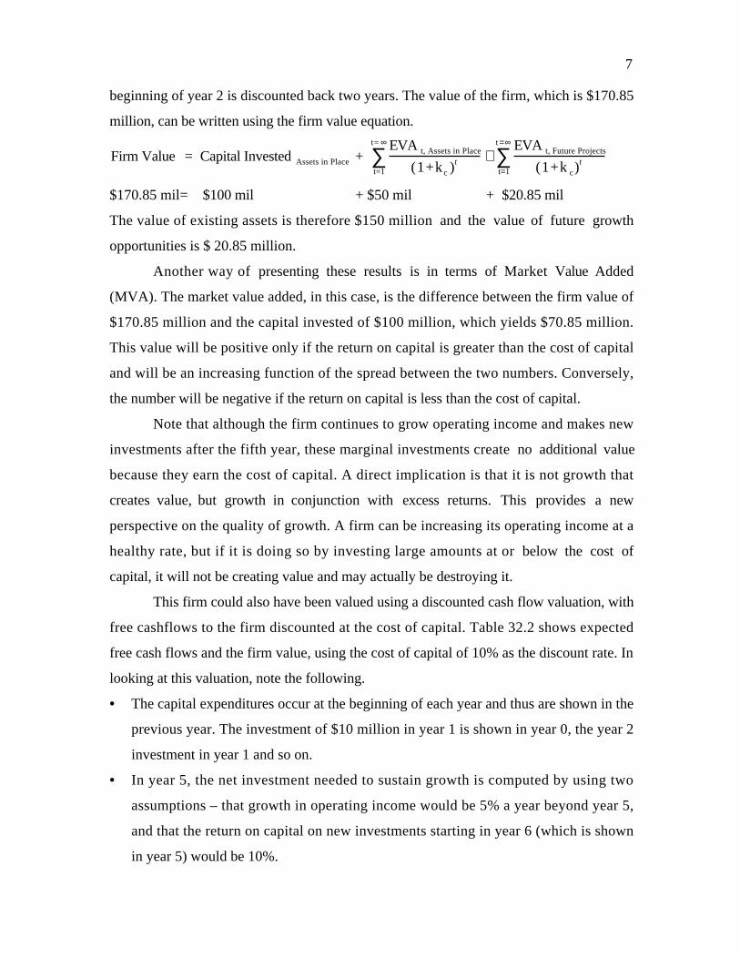
Illustration 32.1: Discounted Cashflow Value and Economic Value Added

Consider a firm that has existing assets in which it has capital invested of $100

million. Assume these additional facts about the firm.

1. The after-tax operating income on assets in place is $15 million. This return on capital

of 15% is expected to be sustained in the future and the company has a cost of capital

of 10%.

2. At the beginning of each of the next 5 years, the firm is expected to make investments

of $10 million each. These investments are also expected to earn 15% as a return on

capital and the cost of capital is expected to remain 10%.

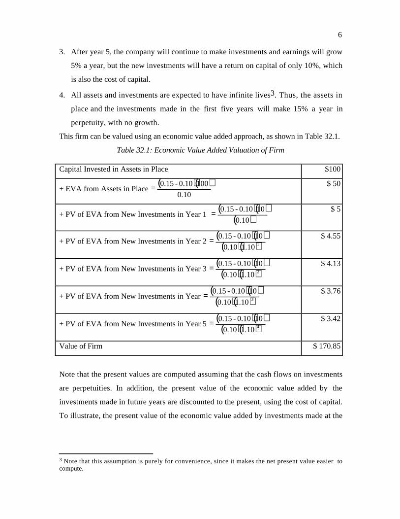
6

3. After year 5, the company will continue to make investments and earnings will grow

5% a year, but the new investments will have a return on capital of only 10%, which

is also the cost of capital.

4. All assets and investments are expected to have infinite lives3. Thus, the assets in

place and the investments made in the first five years will make 15% a year in

perpetuity, with no growth.

This firm can be valued using an economic value added approach, as shown in Table 32.1.

Table 32.1: Economic Value Added Valuation of Firm

Capital Invested in Assets in Place $100

+ EVA from Assets in Place ( )( )

10.01000.10-0.15= $ 50

+ PV of EVA from New Investments in Year 1 ( )( )

( )10.0100.10-0.15= $ 5


( )( )110.110.0100.10-0.15= $ 4.55

+ PV of EVA from New Investments in Year 3 ( )( )( )( )210.110.0

100.10-0.15= $ 4.13

+ PV of EVA from New Investments in Year ( )( )( )( )310.110.0

100.10-0.15= $ 3.76

+ PV of EVA from New Investments in Year 5 ( )( )( )( )410.110.0

100.10-0.15= $ 3.42

Value of Firm $ 170.85

Note that the present values are computed assuming that the cash flows on investments

are perpetuities. In addition, the present value of the economic value added by the

investments made in future years are discounted to the present, using the cost of capital.

To illustrate, the present value of the economic value added by investments made at the

3 Note that this assumption is purely for convenience, since it makes the net present value easier tocompute.

7

beginning of year 2 is discounted back two years. The value of the firm, which is $170.85

million, can be written using the firm value equation.

Firm Value = Capital Invested Assets in Place + EVA t, Assets in Place

(1+k c )tt=1

t= ∞

∑ +EVA t, Future Projects

(1+k c)t

t=1

t =∞

∑

$170.85 mil= $100 mil + $50 mil + $20.85 mil

The value of existing assets is therefore $150 million and the value of future growth

opportunities is $ 20.85 million.

Another way of presenting these results is in terms of Market Value Added

(MVA). The market value added, in this case, is the difference between the firm value of

$170.85 million and the capital invested of $100 million, which yields $70.85 million.

This value will be positive only if the return on capital is greater than the cost of capital

and will be an increasing function of the spread between the two numbers. Conversely,

the number will be negative if the return on capital is less than the cost of capital.

Note that although the firm continues to grow operating income and makes new

investments after the fifth year, these marginal investments create no additional value

because they earn the cost of capital. A direct implication is that it is not growth that

creates value, but growth in conjunction with excess returns. This provides a new

perspective on the quality of growth. A firm can be increasing its operating income at a

healthy rate, but if it is doing so by investing large amounts at or below the cost of

capital, it will not be creating value and may actually be destroying it.

This firm could also have been valued using a discounted cash flow valuation, with

free cashflows to the firm discounted at the cost of capital. Table 32.2 shows expected

free cash flows and the firm value, using the cost of capital of 10% as the discount rate. In

looking at this valuation, note the following.

• The capital expenditures occur at the beginning of each year and thus are shown in the

previous year. The investment of $10 million in year 1 is shown in year 0, the year 2

investment in year 1 and so on.

• In year 5, the net investment needed to sustain growth is computed by using two

assumptions – that growth in operating income would be 5% a year beyond year 5,

and that the return on capital on new investments starting in year 6 (which is shown

in year 5) would be 10%.

8

Net Investment5 ( ) ( )

million 25.11$10.0

50.22$625.23$ROC

1EBIT1EBIT

6

56 =−=−−−= tt

The value of the firm obtained by discounting free cash flows to the firm at the

cost of capital is $170.85, which is identical to the value obtained using the economic

value added approach.

9

Table 32.2: Firm Value using DCF Valuation

0 1 2 3 4 5 Term. Year

EBIT (1-t) from Assets in Place $0.00 $ 15.00 $ 15.00 $ 15.00 $ 15.00 $ 15.00

EBIT(1-t) from Investments - Yr 1 $ 1.50 $ 1.50 $ 1.50 $ 1.50 $ 1.50

EBIT(1-t) from Investments - Yr 2 $ 1.50 $ 1.50 $ 1.50 $ 1.50

EBIT(1-t) from Investments - Yr 3 $ 1.50 $ 1.50 $ 1.50

EBIT(1-t) from Investments - Yr 4 $ 1.50 $ 1.50

EBIT(1-t) from Investments - Yr 5 $ 1.50

Total EBIT(1-t) $ 16.50 $ 18.00 $ 19.50 $ 21.00 $ 22.50 $ 23.63

- Net Capital Expenditures $10.00 $ 10.00 $ 10.00 $ 10.00 $ 10.00 $ 11.25 $ 11.81

FCFF ($10) $ 6.50 $ 8.00 $ 9.50 $ 11.00 $ 11.25 $ 11.81

PV of FCFF ($10) $ 5.91 $ 6.61 $ 7.14 $ 7.51 $ 6.99

Terminal Value $ 236.25

PV of Terminal Value $ 146.69

Value of Firm $170.85

Return on Capital 15% 15% 15% 15% 15% 15% 10%

Cost of Capital 10% 10% 10% 10% 10% 10% 10%

10

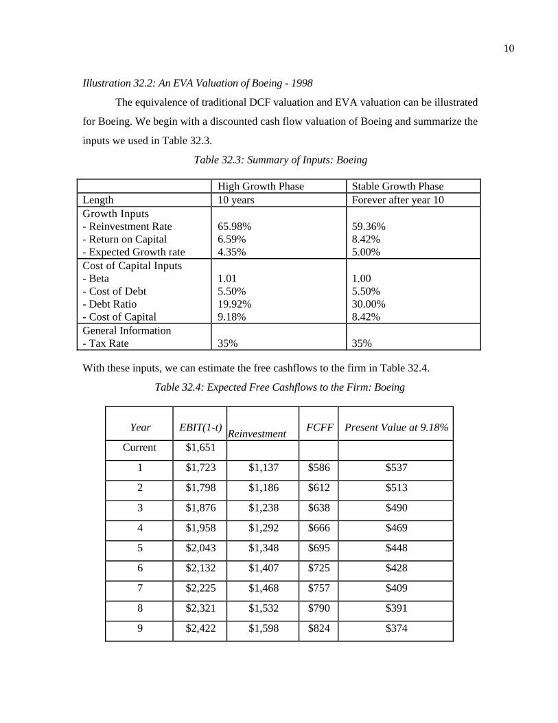
Illustration 32.2: An EVA Valuation of Boeing - 1998

The equivalence of traditional DCF valuation and EVA valuation can be illustrated

for Boeing. We begin with a discounted cash flow valuation of Boeing and summarize the

inputs we used in Table 32.3.

Table 32.3: Summary of Inputs: Boeing

High Growth Phase Stable Growth PhaseLength 10 years Forever after year 10Growth Inputs- Reinvestment Rate- Return on Capital- Expected Growth rate

65.98%6.59%4.35%

59.36%8.42%5.00%

Cost of Capital Inputs- Beta- Cost of Debt- Debt Ratio- Cost of Capital

1.015.50%19.92%9.18%

1.005.50%30.00%8.42%

General Information- Tax Rate 35% 35%

With these inputs, we can estimate the free cashflows to the firm in Table 32.4.

Table 32.4: Expected Free Cashflows to the Firm: Boeing

Year EBIT(1-t) Reinvestment FCFF Present Value at 9.18%

Current $1,651

1 $1,723 $1,137 $586 $537

2 $1,798 $1,186 $612 $513

3 $1,876 $1,238 $638 $490

4 $1,958 $1,292 $666 $469

5 $2,043 $1,348 $695 $448

6 $2,132 $1,407 $725 $428

7 $2,225 $1,468 $757 $409

8 $2,321 $1,532 $790 $391

9 $2,422 $1,598 $824 $374

11

10 $2,528 $1,668 $860 $357

Terminal year $2,654 $1,575 $1,078

The sum of the present value of the cash flows over the growth period is $4,416 million.

The terminal value can be estimated based upon the cash flow in the terminal year and the

cost of capital of 8.42%.

Terminal value million 31,529$05.00842.0

078,1 =−

=

The discounted cash flow estimate of the value is shown below:

Value of Boeing’s operating assets 17,516$0918.1

529,31416,4 10 =+=

In Table 32.5, we estimate the EVA for Boeing each year for the next 10 years,

and the present value of the EVA. To make these estimates, we begin with the current

capital invested in the firm of $26,149 million and add the reinvestment each year from

Table 32.4 to obtain the capital invested in the following year.

Table 32.5: Present Value of EVA at Boeing

Year Capital Invested at beginning

of year

Return on

Capital

Cost of

Capital

EVA PV of EVA

1 $26,149 6.59% 9.18% ($678) ($621)

2 $27,286 6.59% 9.18% ($707) ($593)

3 $28,472 6.59% 9.18% ($738) ($567)

4 $29,710 6.59% 9.18% ($770) ($542)

5 $31,002 6.59% 9.18% ($804) ($518)

6 $32,350 6.59% 9.18% ($839) ($495)

7 $33,757 6.59% 9.18% ($875) ($473)

8 $35,225 6.59% 9.18% ($913) ($452)

9 $36,756 6.59% 9.18% ($953) ($432)

10 $38,354 6.59% 9.18% ($994) ($413)

PV of EVA over 10 years = ($5,107)

The sum of the present values of the EVA is -$5,107 million. To get to the value of the

operating assets of the firm, we add two more components.

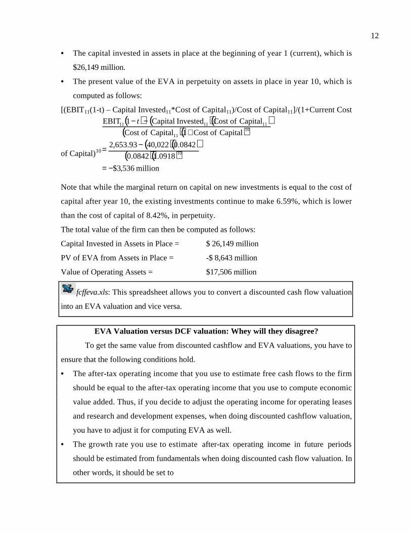
12

• The capital invested in assets in place at the beginning of year 1 (current), which is

$26,149 million.

• The present value of the EVA in perpetuity on assets in place in year 10, which is

computed as follows:

[(EBIT11(1-t) – Capital Invested11*Cost of Capital11)/Cost of Capital11]/(1+Current Cost

of Capital)10

( ) ( )( )( )( )

( )( )( )( )

million 536,3$

0918.10842.00842.0022,4093.653,2

Capital ofCost 1Capital ofCost Capital ofCost Invested Capital1EBIT

10

1011

111111

−=

−=

+−− t

Note that while the marginal return on capital on new investments is equal to the cost of

capital after year 10, the existing investments continue to make 6.59%, which is lower

than the cost of capital of 8.42%, in perpetuity.

The total value of the firm can then be computed as follows:

Capital Invested in Assets in Place = $ 26,149 million

PV of EVA from Assets in Place = -$ 8,643 million

Value of Operating Assets = $17,506 million

fcffeva.xls: This spreadsheet allows you to convert a discounted cash flow valuation

into an EVA valuation and vice versa.

EVA Valuation versus DCF valuation: Whey will they disagree?

To get the same value from discounted cashflow and EVA valuations, you have to

ensure that the following conditions hold.

• The after-tax operating income that you use to estimate free cash flows to the firm

should be equal to the after-tax operating income that you use to compute economic

value added. Thus, if you decide to adjust the operating income for operating leases

and research and development expenses, when doing discounted cashflow valuation,

you have to adjust it for computing EVA as well.

• The growth rate you use to estimate after-tax operating income in future periods

should be estimated from fundamentals when doing discounted cash flow valuation. In

other words, it should be set to

13

Growth rate = Reinvestment rate * Return on capital

If growth is an exogenous input into a DCF model and the relationship between growth

rates, reinvestments and return on capital outlined above does not hold, you will get

different values from DCF and EVA valuations.

• The capital invested, which is used to compute EVA in future periods, should be

estimated by adding the reinvestment in each period to the capital invested at the

beginning of the period. The EVA in each period should be computed as follows:

EVAt = After-tax Operating Incomet – Cost of capital* Capital Investedt-1

• You have to make consistent assumptions about terminal value in your discounted

cash flow and EVA valuations. In the special case, where the return on capital on all

investments – existing and new - is equal to the cost of capital after your terminal

year, this is simple to do. The terminal value will be equal to your capital invested at

the beginning of your terminal year. In the more general case, you will have to ensure

that the capital invested at the beginning of your terminal year is consistent with your

assumption about return on capital in perpetuity. In other words, if your after-tax

operating income in your terminal year is $1.2 billion and you are assuming a return

on capital of 10% in perpetuity, you will have to set your capital invested at the

beginning of your terminal year to be $12 billion.

EVA and Firm Value: Potential Conflicts

Assume that a firm adopts economic value added as its measure of value and

decides to judge managers on their capacity to generate greater-than-expected economic

value added. What is the potential for abuse? Is it possible for a manager to deliver greater

than expected economic value added, while destroying firm value at the same time? If so,

how can we protect stockholders against these practices?

To answer these questions, let us go back to the earlier equation where we

decomposed firm value into capital invested, the present value of economic value added

by assets in place and the present value of economic value added by future growth.

∑∑∞=

=

∞ t

1t c

Projects Future t,=t

=1t c

Placein Assets t,Placein Assets

)k+(1

EVA+

)k+(1

EVA+Invested Capital=Value Firm tt

14

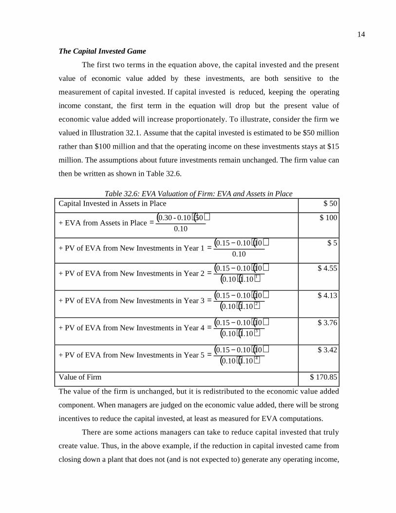
The Capital Invested Game

The first two terms in the equation above, the capital invested and the present

value of economic value added by these investments, are both sensitive to the

measurement of capital invested. If capital invested is reduced, keeping the operating

income constant, the first term in the equation will drop but the present value of

economic value added will increase proportionately. To illustrate, consider the firm we

valued in Illustration 32.1. Assume that the capital invested is estimated to be $50 million

rather than $100 million and that the operating income on these investments stays at $15

million. The assumptions about future investments remain unchanged. The firm value can

then be written as shown in Table 32.6.

Table 32.6: EVA Valuation of Firm: EVA and Assets in PlaceCapital Invested in Assets in Place $ 50


10.0500.10-0.30= $ 100


10.01010.015.0 −= $ 5


( )( )110.110.01010.015.0 −= $ 4.55


( )( )210.110.01010.015.0 −= $ 4.13


( )( )310.110.01010.015.0 −= $ 3.76


( )( )410.110.01010.015.0 −= $ 3.42


The value of the firm is unchanged, but it is redistributed to the economic value added

component. When managers are judged on the economic value added, there will be strong

incentives to reduce the capital invested, at least as measured for EVA computations.

There are some actions managers can take to reduce capital invested that truly

create value. Thus, in the above example, if the reduction in capital invested came from

closing down a plant that does not (and is not expected to) generate any operating income,

15

the cash flow generated by liquidating the plant’s assets will increase value. Some actions,

however, are purely cosmetic in terms of their effects on capital invested and thus do not

create and may even destroy value. For instance, firms can take one-time restructuring

charges, reducing capital or lease assets rather than buy them, because the capital impact

of leasing may be smaller.

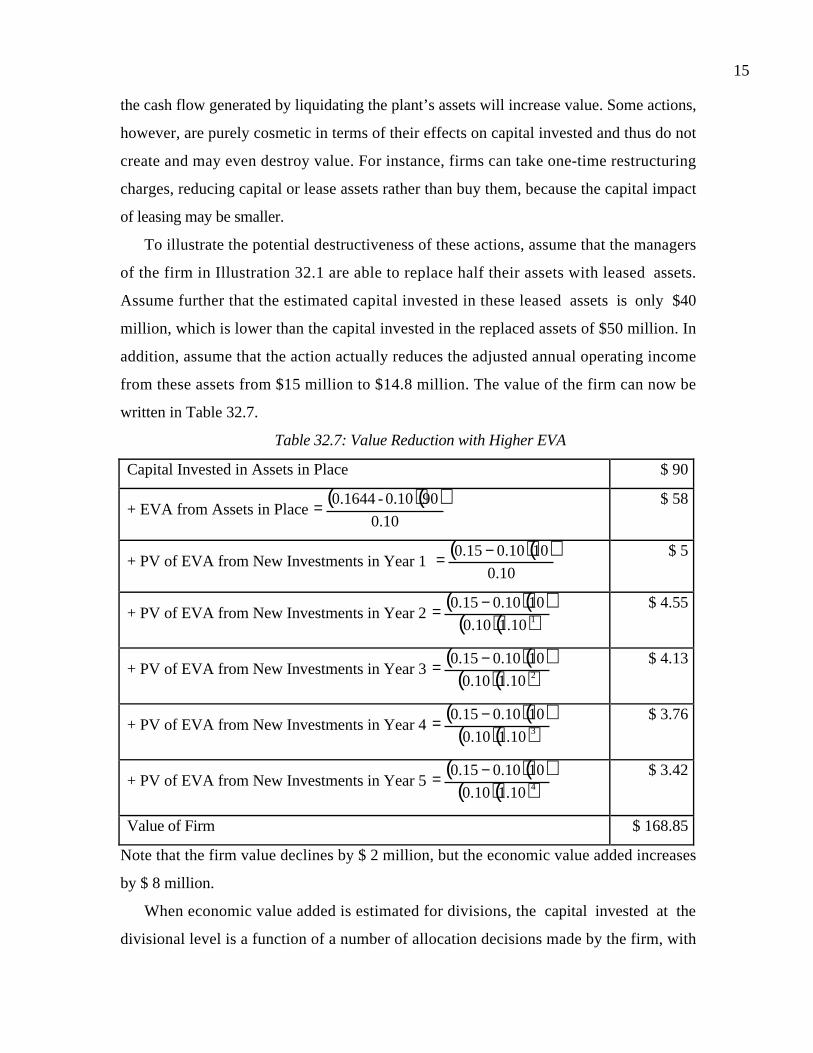
To illustrate the potential destructiveness of these actions, assume that the managers

of the firm in Illustration 32.1 are able to replace half their assets with leased assets.

Assume further that the estimated capital invested in these leased assets is only $40

million, which is lower than the capital invested in the replaced assets of $50 million. In

addition, assume that the action actually reduces the adjusted annual operating income

from these assets from $15 million to $14.8 million. The value of the firm can now be

written in Table 32.7.

Table 32.7: Value Reduction with Higher EVA

Capital Invested in Assets in Place $ 90


10.0900.10-0.1644= $ 58


10.01010.015.0 −= $ 5


( )( )110.110.01010.015.0 −= $ 4.55


( )( )210.110.01010.015.0 −= $ 4.13


( )( )310.110.01010.015.0 −= $ 3.76


( )( )410.110.01010.015.0 −= $ 3.42


Note that the firm value declines by $ 2 million, but the economic value added increases

by $ 8 million.

When economic value added is estimated for divisions, the capital invested at the

divisional level is a function of a number of allocation decisions made by the firm, with

16

the allocation based upon pre-specified criteria (such as revenues or number of

employees). While we would like these rules to be objective and unbiased, they are often

subjective and over allocate capital to some divisions and under-allocate it to others. If

this misallocation were purely random, we could accept it as error and use changes in

economic value added to measure success. Given the natural competition that exists

among divisions in a firm for the marginal investment dollar, however, these allocations

are also likely to reflect the power of individual divisions to influence the process. Thus,

the economic value added will be over-estimated for those divisions that are under

allocated capital and under-estimated for divisions that are over-allocated capital.

The Future Growth Game

The value of a firm is the value of its existing assets and the value of its future

growth prospects. When managers are judged on the basis of economic value added in the

current year, or on year-to-year changes, the economic value added that is being measured

is just from assets in place. Thus, managers may trade off the economic value added from

future growth for higher economic value added from assets in place.

Again, this point can be illustrated simply using the firm in Illustration 32.1. The

firm earned a return on capital of 15% on both assets in place and future investments.

Assume that there are actions the firm can take to increase the return on capital on assets

in place to 16%, but that this action reduces the return on capital on future investments to

12%. The value of this firm can then be estimated in Table 32.8:

Table 32.8: Trading Off Future Growth for Higher EVACapital Invested in Assets in Place $ 100


10.01000.10-0.16= $ 60


10.01010.012.0 −= $ 2


( )( )1.110.01010.012.0 −= $ 1.82


( )( )21.110.01010.012.0 −= $ 1.65

17


( )( )31.110.01010.012.0 −= $ 1.50


( )( )41.110.01010.012.0 −= $ 1.37


Note that the value of the firm has decreased, but the economic value added in year 1 is

higher now than it was before. In fact, the economic value added at this firm for each of

the next five years is graphed in Figure 32.1 for both the original firm and this one.

The growth trade off, while leading to a lower firm value, results in economic value added

in each of the first three years that is larger than it would have been without the trade off.

Compensation mechanisms based upon EVA are sometimes designed to punish

managers who give up future growth for current EVA. Managers are partly compensated

based upon the economic value added this year, but another part is held back in a

compensation bank and is available to the manager only after a period (say three or four

years). There are significant limitations with these approaches. First, the limited tenure

that managers have with firms implies that this measure can at best look at economic

Figure 32.1: Annual EVA: With and Without Growth Trade-Off

$-

$1.00

$2.00

$3.00

$4.00

$5.00

$6.00

$7.00

$8.00

1 2 3 4 5

Year

EV

A EVA (Original)EVA (Growth Trade-Off)

18

value added only over the next 3 or 4 years. The real costs of the growth trade off are

unlikely to show up until much later. Second, these approaches are really designed to

punish managers who increase economic value added in the current period while reducing

economic value added in future periods. In the more subtle case, where the economic value

added continues to increase but at a rate lower than it otherwise would have, it is difficult

to devise a punishment for managers who trade off future growth. In the example above,

for instance, the economic value added with the growth trade off increases over time. The

increases are smaller than they would have been without the trade off, but that number

would not have been observed anyway.

The Risk Shifting Game

The value of a firm is the sum of the capital invested and the present value of the

economic value added. The latter term is therefore a function not just of the dollar

economic value added but also of the cost of capital. A firm can invest in projects to

increase its economic value added but still end up with a lower value, if these investments

increase its operating risk and cost of capital.

Again, using the firm in Illustration 32.1, assume that the firm is able to increase

its return on capital on both assets in place and future investments from 15% to 16.25%.

Simultaneously, assume that the cost of capital increases to 11%. The economic value

added in each year for the next five years is contrasted with the original economic value

added in each year in Figure 32.2.

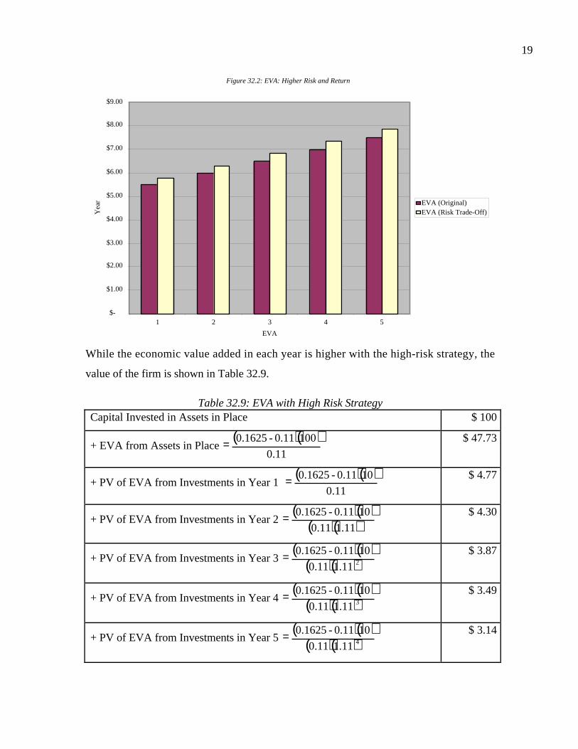
19

While the economic value added in each year is higher with the high-risk strategy, the

value of the firm is shown in Table 32.9.

Table 32.9: EVA with High Risk StrategyCapital Invested in Assets in Place $ 100


11.01000.11-0.1625= $ 47.73

+ PV of EVA from Investments in Year 1 ( )( )

11.0100.11-0.1625= $ 4.77


( )( )11.111.0100.11-0.1625= $ 4.30


( )( )211.111.0100.11-0.1625= $ 3.87


( )( )311.111.0100.11-0.1625= $ 3.49


( )( )411.111.0100.11-0.1625= $ 3.14

Figure 32.2: EVA: Higher Risk and Return

$-

$1.00

$2.00

$3.00

$4.00

$5.00

$6.00

$7.00

$8.00

$9.00

1 2 3 4 5

EVA

Yea

r EVA (Original)EVA (Risk Trade-Off)

20


Note that the risk effect dominates the higher excess dollar returns and the value of the

firm decreases.

This risk shifting can be dangerous for firms that adopt economic value added

based on objective functions. When managers are judged based upon year-to-year

economic value added changes, there will be a tendency to shift into riskier investments.

This tendency will be exaggerated if the measured cost of capital does not reflect the

changes in risk or lags4 it.

In closing, economic value added is an approach skewed toward assets in place

and away from future growth. It should not be surprising, therefore, that when economic

value added is computed at the divisional level of a firm, the higher growth divisions end

up with the lowest economic value added and in some cases with negative economic value

added. Again, while these divisional managers may still be judged based upon changes in

economic value added from year to year, the temptation at the firm level to reduce or

eliminate capital invested in these divisions will be strong, since it will make the firm’s

overall economic value added look much better.

EVA and Market Value

Will increasing economic value added cause market value to increase? While an

increase in economic value added will generally lead to an increase in firm value, barring

the growth and risk games described earlier, it may or may not increase the stock price.

This is because the market has built into its expectations of future economic value added.

Thus, a firm like Microsoft is priced on the assumption that it will earn large and

increasing economic value added over time. Whether a firm’s market value increases or

decreases on the announcement of higher economic value added will depend in large part

on what the expected change in economic value added was. For mature firms, where the

market might have expected no increase or even a decrease in economic value added, the

announcement of an increase will be good news and cause the market value to increase.

4 In fact, beta estimates that are based upon historical returns will lag changes in risk. With a five-yearreturn estimation period, for instance, the lag might be as long as three years and the full effect will notshow up for five years after the change.

21

For firms that are perceived to have good growth opportunities and are expected to report

an increase in economic value added, the market value will decline if the announced

increase in economic value added does not measure up to expectations. This should be no

surprise to investors, who have recognized this phenomenon with earnings per share for

decades; the earnings announcements of firms are judged against expectations and the

earnings surprise is what drives prices.

We would therefore not expect any correlation between the magnitude of the

economic value added and stock returns or even between the change in economic value

added and stock returns. Stocks that report the biggest increases in economic value added

should not necessarily earn high returns for their stockholders5. These priors are

confirmed by a study done by Richard Bernstein at Merrill Lynch, who examined the

relationship between EVA and stock returns.

• A portfolio of the 50 firms which had the highest absolute levels6 of economic value

added earned an annual return on 12.9% between February 1987 and February 1997,

while the S&P index returned 13.1% a year over the same period.

• A portfolio of the 50 firms that had the highest growth rates7 in economic value

added over the previous year earned an annual return of 12.8% over the same time

period.

eva.xls: There is a dataset on the web that summarizes economic value added by

industry group for the United States.

Equity Economic Value Added

While EVA is usually calculated using total capital, it can easily be modified to be

an equity measure.

Equity EVA = (Return on Equity - Cost of Equity) (Equity Invested in Project or Firm)

= Net Income – (Cost of Equity)(Equity Invested in Project or Firm)

5 A study by Kramer and Pushner found that differences in operating income (NOPAT) explained differencesin market value better than differences in EVA. O'Byrne (1996), however, finds that changes in EVAexplain more than 55% of changes in market value over 5-year periods.6 See Quantitative Viewpoint, Merrill Lynch, December 19, 1997.

22

Again, a firm that earns a positive equity EVA is creating value for its stockholders while

a firm with a negative equity EVA is destroying value for its stockholders.

Why might a firm use this measure rather than the traditional measure? In Chapter

21, when we looked at financial service firms, we noted that defining debt (and therefore

capital) may create measurement problems, since so much of the firm could potentially be

categorized as debt. Consequently, we argued that financial service firms should be valued

using equity valuation models and multiples. Extending that argument to economic value

added, we believe that equity EVA is a much better measure of performance for financial

service firms than the traditional EVA measure.

We would hasten to add that all of the issues that we raised in the context of the

traditional EVA measure affect the equity EVA measure as well. Banks and insurance

companies can play the capital invested, growth and risk games to increase equity EVA

just as other firms can with traditional EVA.

EVA for High Growth firms

The fact that the value of a firm is a function of the capital invested in assets in

place, the present value of economic value added by those assets and the economic value

added by future investments, points to some of the dangers of using it as a measure of

success or failure for high growth and especially high-growth technology firms. In

particular, there are three problems.

• We have already noted many of the problems associated with how accountants

measure capital invested at technology firms. Given the centrality of capital invested

to economic value added, these problems have a much bigger effect when firms use

EVA than when discounted cash flow valuation.

• When 80% to 90% of value comes from future growth potential, the risks of managers

trading off future growth for current EVA are magnified. It is also very difficult to

monitor these trade offs at young firms.

7 See Quantitative Viewpoint, Merrill Lynch, February 3, 1998.

23

• The constant change that these firms go through also makes them much better

candidates for risk shifting. In this case, the negative effect (of a higher discount rate)

can more than offset the positive effect of a higher economic value added.

Finally, it is unlikely that there will be much correlation between actual changes in

economic value added at technology firms and changes in market value. The market value

is based upon expectations of economic value added in future periods and investors

expect an economic value added that grows substantially each year. Thus, if the economic

value added increases, but by less than expected, you could see its market value drop on

the report.

Cash Flow Return on Investment

The cash flow return on investment (CFROI) for a firm is the internal rate of

return on existing investments, based upon real cash flows. Generally, it should be

compared to the real cost of capital to make judgments about the quality of these

investments.

Calculating CFROI

The cash flow return on investment for a firm is calculated using four inputs. The

first is the gross investment (GI) the firm has in its existing assets, obtained by adding

back cumulated depreciation and inflation adjustments to the book value. The second

input is the gross cash flow (GCF) earned in the current year on gross investment, which

is usually defined as the sum of the after-tax operating income of a firm and the non-cash

charges against earnings, such as depreciation and amortization. The third input is the

expected life of the assets (n) in place at the time of the original investment, which varies

from sector to sector but reflects the earning life of the investments in question. The

expected value of the assets (SV) at the end of this life, in current dollars, is the final input.

This is usually assumed to be the portion of the initial investment, such as land and

building, that is not depreciable, adjusted to current dollar terms. The CFROI is the

internal rate of return of these cash flows, i.e, the discount rate that makes the net present

value of the gross cash flows and salvage value equal to the gross investment and it can

thus be viewed as a composite internal rate of return, in current dollar terms.

24

An alternative formulation of the CFROI allows for setting aside an annuity to

cover the expected replacement cost of the asset at the end of the project life. This

annuity is called the economic depreciation.

( ) 1k+1)(k dollarsCurrent in Cost t Replacemen

=onDepreciati Economic nc

c

−

where n is the expected life of the asset. The expected replacement cost of the asset is

defined in current dollar terms to be the difference between the gross investment and the

salvage value. The CFROI for a firm or a division can then be written as follows:

Investment GrossonDepreciati Economic-FlowCash Gross

=CFROI

For instance, assume that you have existing assets with a book value of $2,431 million, a

gross cash flow of $390 million, an expected salvage value (in today’s dollar terms) of

$607.8 million and a life of 10 years. The conventional measure of CFROI is 11.71% and

the real cost of capital is 8%. The estimate using the alternative approach is computed.

( )( )million 86.125$

11.080.08$607.8 - $2,431

onDepreciati Economic 10 =−

=

10.87%2,431

125.86-390CFROI ==

The differences in the reinvestment rate assumption accounts for the difference in CFROI

estimated using the two methods. In the first approach, intermediate cash flows get

reinvested at the internal rate of return, while in the second, at least the portion of the

cash flows that are set aside for replacement get reinvested at the cost of capital. In fact, if

we estimated that the economic depreciation using the internal rate of return of 11.71%,

the two approaches would yield identical results8.

8 With an 11.71% rate, the economic depreciation works out to $105.37 million and the CFROI to11.71%.

25

Cashflow Return on Investment, Internal Rate of Return and Discounted Cashflow

Value

If net present value provides the genesis for the economic value added approach to

value enhancement, the internal rate of return is the basis for the CFROI approach. In

investment analysis, the internal rate of return on a project is computed using the initial

investment on the project and all cash flows over the project’s life.

InitialInvestment

ATCF ATCF ATCF ATCF ATCF

1 2 3 4 n

SV

Where the ATCF is the after-tax cash flow on the project and SV is the expected salvage

value of the project assets. This analysis can be done entirely in nominal terms, in which

case the internal rate of return is a nominal IRR and is compared to the nominal cost of

capital, or in real terms, in which case it is a real IRR and is compared to the real cost of

capital.

At first sight, the CFROI seems to do the same thing as IRR. It uses the gross

investment in the project (in current dollars) as the equivalent of the initial investment,

assumes that the gross current-dollar cash flow is maintained over the project life and

computes a real internal rate of return. There are, however, some significant differences.

The internal rate of return does not require the after-tax cash flows to be constant

over a project’s life, even in real terms. The CFROI approach assumes that real cash

flows on assets do not increase over time. This may be a reasonable assumption for

investments in mature markets, but will understate project returns if there is real growth.

Note, however, that the CFROI approach can be modified to allow for real growth.

The second difference is that the internal rate of return on a project or asset is

based upon incremental future cash flows. It does not consider cash flows that have

occurred already, since these are viewed as “sunk.” The CFROI, on the other hand, tries

to reconstruct a project or asset, using both cash flows that have occurred already and

cashflows that are yet to occur. To illustrate, consider the project described in the

previous section. At the time of the original investment, assuming that the inputs for

initial investment, after-tax cash flows and salvage value are unchanged, both the internal

26

rate of return and the CFROI of this project would have been 11.71%. The CFROI is,

however, being computed three years into the project life and remains at 11.71%, since

none of the original inputs have changed. The IRR of this project will change, though. It

will now be based upon the current market value of the asset, the expected cash flows

over the remaining life of the asset and a life of seven years. Thus, if the market value of

the asset has increased to $2.5 billion, the internal rate of return on this project would be

computed to be only 6.80%.

$ 3,000 mil

$390 mil $390 mil $390 mil $390 mil $ 390 mil

1 2 3 4 7

$607.8 mil

Given the real cost of capital of 8%, this would mean that the CFROI is greater than the

cost of capital, while the internal rate of return is lower. Why is there a difference

between the two measures and what are the implications? The reason for the difference is

that IRR is based entirely on expected future cash flows, whereas the CFROI is not. A

CFROI that exceeds the cost of capital is viewed as a sign that a firm is deploying its

assets well. If the IRR is less than the cost of capital, that interpretation is false, because

the owners of the firm would be better off selling the asset and getting the market value

for it rather than continuing its operation.

To link the cash flow return on investment with firm value, let us begin with a

simple discounted cash flow model for a firm in stable growth.

nc

1

gkFCFF

=Value Firm−

where FCFF is the expected free cash flow to the firm, kc is the cost of capital and gn is

the stable growth rate. Note that this can be rewritten, approximately, in terms of the

CFROI.

( )( )( )( ) ( )nc gk

WC-DA-CXt-1DA-GICFROI=Value Firm

−∆−

where CFROI is the cash flow return on investment, GI is the gross investment, DA is

the depreciation and amortization, CX is the capital expenditure and ∆WC is the change in

27

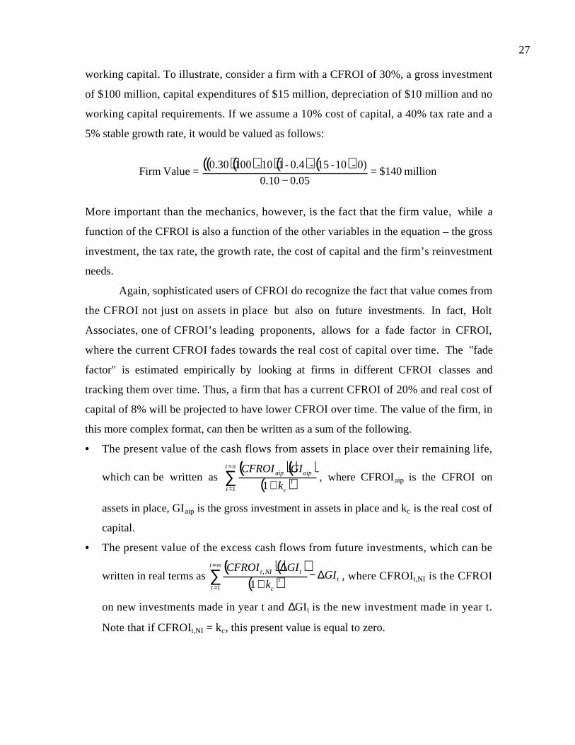
working capital. To illustrate, consider a firm with a CFROI of 30%, a gross investment

of $100 million, capital expenditures of $15 million, depreciation of $10 million and no

working capital requirements. If we assume a 10% cost of capital, a 40% tax rate and a

5% stable growth rate, it would be valued as follows:

( )( )( )( ) ( )million $140=

05.00.10)0-10-15-0.4-110-1000.30

=Value Firm−

More important than the mechanics, however, is the fact that the firm value, while a

function of the CFROI is also a function of the other variables in the equation – the gross

investment, the tax rate, the growth rate, the cost of capital and the firm’s reinvestment

needs.

Again, sophisticated users of CFROI do recognize the fact that value comes from

the CFROI not just on assets in place but also on future investments. In fact, Holt

Associates, one of CFROI’s leading proponents, allows for a fade factor in CFROI,

where the current CFROI fades towards the real cost of capital over time. The "fade

factor" is estimated empirically by looking at firms in different CFROI classes and

tracking them over time. Thus, a firm that has a current CFROI of 20% and real cost of

capital of 8% will be projected to have lower CFROI over time. The value of the firm, in

this more complex format, can then be written as a sum of the following.

• The present value of the cash flows from assets in place over their remaining life,

which can be written as ( )( )

( )∑=

= +

nt

tt

c

aipaip

k

GICFROI

1 1, where CFROIaip is the CFROI on

assets in place, GIaip is the gross investment in assets in place and kc is the real cost of

capital.

• The present value of the excess cash flows from future investments, which can be

written in real terms as ( )( )

( ) t

t

tt

c

tNIt GIk

GICFROI∆−

+∆∑

∞=

=1

,

1, where CFROIt,NI is the CFROI

on new investments made in year t and ∆GIt is the new investment made in year t.

Note that if CFROIt,NI = kc, this present value is equal to zero.

28

Thus, a firm's value will depend upon the CFROI it earns on assets in place and both the

abruptness and the speed with which this CFROI fades towards the cost of capital. Thus,

a firm can therefore potentially increase its value by doing any of the following.

• Increase the CFROI from assets in place, for a given gross investment.

• Reduce the speed at which the CFROI fades towards the real cost of capital.

• Reduce the abruptness with which CFROI fades towards the cost of capital.

Note that this is no different from our earlier analysis of firm value in the

discounted cash flow approach, in terms of cash flows from existing investments (increase

current CFROI), the length of the high growth period (reduce fade speed) and the growth

rate during the growth period (keep excess returns from falling as steeply).

cfroi.xls: This spreadsheet allows you to estimate the cash flow return on investment

for a firm or project.

CFROI Innovations: The Fade Factor and Implied Cost of Capital

The biggest contribution made by practitioners who use CFROI has been the

work that they have done on how returns on capital fade over time towards the cost of

capital. Madden (1999) makes the argument that not only is this phenomenon wide

spread but that it is at least partially predictable. He presents evidence done by Holt

Associates, a leading proponent of CFROI, who sorted the largest 1000 firms by CFROI,

from highest to lowest and tracked them over time, to find a convergence towards an

average. We should note that we have used fade factors, without referring to them as such,

in the chapters on discounted cash flow valuation. The fade to a lower return on capital

occurred either precipitously in the terminal year or over a transition period. We noted

that the return on capital could converge to the cost of capital or to the industry average.

To compute the cost of capital, CFROI practitioners look to the market instead of

the risk and return models that we have used to compute DCF value. Using the current

market values of stocks and their estimates of expected aggregate cash flows, they

compute internal rates of return that they use as the cost of capital in analysis. In Chapter

7, we used a very similar approach to estimate an implied risk premium, though we use

this premium as an input into traditional risk and return models.

29

CFROI and Firm Value: Potential Conflicts

The relationship between CFROI and firm value is less intuitive than the

relationship between EVA and firm value, partly because it is a percentage return.

Notwithstanding this fundamental weakness, managers can take actions that increase

CFROI while reducing firm value.

a. Reduce Gross Investment: If the gross investment in existing assets is reduced,

the CFROI may be increased. Since it is the product of CFROI and Gross

Investment that determines value, it is possible for a firm to increase CFROI

and end up with a lower value.

b. Sacrifice Future Growth: CFROI, even more than EVA, is focused on existing

assets and does not look at future growth. To the extent that managers increase

CFROI at the expense of future growth, the value can decrease while CFROI

goes up.

c. The Risk Trade Off: While the CFROI is compared to the real cost of capital

to pass judgment on whether a firm is creating or destroying value, it

represents only a partial correction for risk. The value of a firm is still the

present value of expected future cash flows. Thus, a firm can increase its

spread between the CFROI and cost of capital but still end up losing value if

the present value effect of having a higher cost of capital dominates the higher

CFROI.

In general, then, an increase in CFROI does not, by itself, indicate that the firm value has

increased, since it might have come at the expense of lower growth and/or higher risk.

CFROI and Market Value

There is a relationship between CFROI and market value. Firms with high CFROI

generally have high market value. This is not surprising, since it mirrors what we noted

about economic value added earlier. However, it is changes in market value that create

returns, not market value per se. When it comes to market value changes, the relationship

between EVA changes and value changes tends to be much weaker. Since market values

reflect expectations, there is no reason to believe that firms that have high CFROI will

earn excess returns.

30

The relationship between changes in CFROI and excess returns is more intriguing. To the

extent that any increase in CFROI is viewed as a positive surprise, firms with the biggest

increases in CFROI should earn excess returns. In reality, however, the actual change in

CFROI has to be measured against expectations; if CFROI increases, but less than

expected, the market value should drop; if CFROI drops but by less than expected, the

market value should increase.

A Postscript on Value Enhancement

The value of a firm has three components. The first is its capacity to generate cash

flows from existing assets, with higher cash flows translating into higher value. The

second is its willingness to reinvest to create future growth and the quality of these

reinvestments. Other things remaining equal, firms that reinvest well and earn significant

excess returns on these investments will have higher value. The final component of value

is the cost of capital, with higher costs of capital resulting in lower firm values. To create

value then a firm has to:

• Generate higher cash flows from existing assets, without affecting its growth

prospects or its risk profile.

• Reinvest more and with higher excess returns, without increasing the riskiness of its

assets.

• Reduce the cost of financing its assets in place or future growth, without lowering the

returns made on these investments.

All value enhancement measures are variants on these simple themes. Whether these

approaches measure dollar excess returns, as does economic value added, or percentage

excess returns, like CFROI, they have acquired followers because they seem simpler and

less subjective than discounted cash flow valuation. This simplicity comes at a cost, since

these approaches make subtle assumptions about other components of value that are

often not visible or not recognized by many users. Approaches that emphasize economic

value added and reward managers for increasing the same, often assume that increases in

economic value added are not being accomplished at the expense of future growth or by

increasing risk. Practitioners who judge performance based upon the cash flow return on

investment make similar assumptions.

31

Is there something of value in the new value enhancement measures? Absolutely,

but only in the larger context of valuation. One of the inputs we need for traditional

valuation models is the return on capital (to get expected growth). Making the

adjustments to operating income suggested by those who use economic value added and

augmenting it with a cash flow return, with CFROI, may help us come up with a better

estimate of this number. The terminal value computation in traditional valuation models,

where small changes in assumptions can lead to large changes in value, becomes much

more tractable if we think in terms of excess returns on investments rather than just

growth and discount rates. Finally, the empirical evidence that has been collected by

practitioners who use CFROI on fade factors can be invaluable in traditional valuation

models, where practitioners sometimes make the mistake of assuming that current project

returns will continue forever.

Summary

In this chapter, we consider two widely used value enhancement measures.

Economic value added measures the dollar excess return on existing assets. The cash flow

return on investment is the internal rate of return on existing assets, based upon the

original investment in these assets and the expected future cash flows. While both

approaches can lead to conclusions consistent with traditional discounted cash flow

valuation, their simplicity comes at a cost. Managers can take advantage of measurement

limitations in both approaches to make their firms look better with either approach, while

reducing firm value. In particular, they can trade off less growth in the future for higher

economic value added today and shift to riskier investments.

As we look at various approaches to value enhancement, we should consider a few

facts. The first is that no value enhancement mechanism will work at generating value

unless there is a commitment on the part of managers to making value maximization their

primary objective. If managers put other goals first, then no value enhancement

mechanism will work. Conversely, if managers truly care about value maximization, they

can make almost any mechanism work in their favor. The second is that while it is

sensible to connect whatever value enhancement measure we have chosen to management

compensation, there is a down side. Managers, over time, will tend to focus their

32

attention on making themselves look better on that measure even if it leads to reducing

firm value. Finally, there are no magic bullets that create value. Value creation is hard

work in competitive markets and almost involves a trade off between costs and benefits.

Everyone has a role in value creation and it certainly is not the sole domain of financial

analysts. In fact, the value created by financial engineers is smaller and less significant

than the value created by good strategic, marketing, production or personnel divisions.

33

Problems

1. Everlast Batteries Inc. has hired you as a consultant. The firm had after-tax operating

earnings in 1998 of $180 million, net income of $100 million and it paid a dividend of $50

million. The book value of equity at the end of 1998 was $1.25 billion and the book value

of debt was $350 million. The firm raised $50 million of new debt during 1998. The

market value of equity at the end of 1998 was twice the book value of equity and the

market value of debt was the same as the book value of debt. The firm has a cost of

equity of 12% and an after-tax cost of debt of 5%.

a. Estimate the return on capital earned by Everlast Batteries

b. Estimate the cost of capital earned by Everlast Batteries

c. Estimate the economic value added by Everlast Batteries

2. Assume, in the last problem, that Everlast Batteries is in stable growth and that it

expects its economic value added to grow at 5% a year forever.

a. Estimate the value of the firm.

b. How much of this value comes from excess returns?

c. What is the market value added (MVA) of this firm?

c. How would your answers to (a), (b) and (c) change if you were told that there would be

no economic value added after year 5?

3. Stereo City is a retailer of stereos and televisions. The firm has operating income of

$150 million, after operating lease expenses of $50 million. The firm has operating lease

commitments for the next 5 years and beyond.

Year Operating lease commitment

1 55

2 60

3 60

4 55

5 50

yr 6-15 40Each year

34

The book value of equity is $1 billion and the firm has no debt outstanding. The firm has

a cost of equity of 11% and a pre-tax cost of borrowing of 6%. The tax rate is 40%.

a. Estimate the capital invested in the firm, before and after adjusting for operating

leases.

b. Estimate the return on capital, before and after adjusting for operating leases.

c. Estimate the economic value added, before and after adjusting for operating

leases. (The market value of equity is $2 billion.)

4. Sevilla Chemicals earned $1 billion in after-tax operating income on capital invested of

$5 billion last year. The firm’s cost of equity is 12%, its debt to capital ratio is 25% and

the after-tax cost of debt is 4.5%.

a. Estimate the economic value added by Sevilla Chemicals last year.

b. Assume now that the entire chemical industry earned $40 billion after taxes on capital

invested of $180 billion and that the cost of capital for the industry is 10%. Estimate the

economic value added by the entire industry.

c. Based on economic value added, how did Sevilla do, relative to the industry?

5. Jeeves Software is a small software firm in high growth. The firm is all equity financed.

In the current year, the firm earned $20 million in after-tax operating income on capital

invested of $60 million. The firm’s cost of equity is 15%.

a. Assume that the firm will be able to grow its economic value added 15% a year for the

next 5 years and that there will be no excess returns after year 5. Estimate the value of the

firm. How much of this value comes from the EVA and how much from capital invested?

b. Now, assume the firm is able to reduce its capital invested this year by $20 million by

selling its assets and leasing them back. Assuming operating income and cost of capital do

not change as a result of the sale-lease back, estimate the value of the firm now. How

much of the value of the firm now comes from EVA and how much from capital invested?

6. Healthy Soups is a company that manufactures canned soups made without

preservatives. The firm has assets that have a book value of $100 million. The assets are 5

years old and have been depreciated $50 million over that period. In addition, the inflation

rate over those 5 years has averaged 2% a year. The assets are currently earning $15

35

million in after-tax operating income. They have a remaining life of 10 years and the

depreciation each year is expected to be $5 million. At the end of these 10 years, the

assets will have an expected salvage value, in current dollars, of $50 million.

a. Estimate the CFROI of Healthy Foods, using the conventional CFROI approach.

b. Estimate the CFROI of Healthy Foods, using the economic depreciation approach.

c. If Healthy Foods has a cost of capital in nominal terms of 10% and the expected

inflation rate is 2%, evaluate whether Healthy Foods’ existing investments are value

creating or destroying.

value enhancement: eva, cfroi and other …people.stern.nyu.edu/adamodar/pdfiles/valn2ed/ch32.pdf1...

Documents