Valuation 4: Econometrics

• Why econometrics? • What are the tasks?• Specification and estimation• Hypotheses testing• Example study

Last week we looked at

• What is so special about environmental goods?• Theory of consumer demand for market goods• Welfare effects of a price change: Equivalent

variation versus compensating variation• Consumer demand for environmental goods• Welfare effects of a quantity change:

Equivalent surplus versus compensating surplus

• Theory and practise

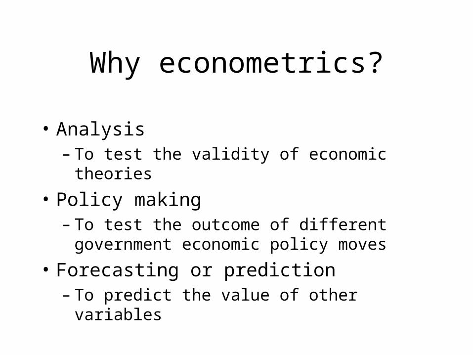
Why econometrics?

• Analysis– To test the validity of economic theories

• Policy making– To test the outcome of different

government economic policy moves

• Forecasting or prediction– To predict the value of other variables

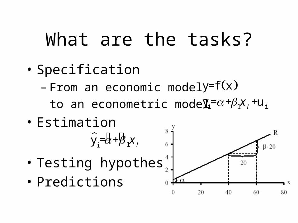
What are the tasks?

• Specification– From an economic model

to an econometric model

• Estimation

• Testing hypotheses• Predictions

y=f x i i1y= + +uix

1iy = + ix

Specification – the function

• Include all relevant exogenous variables• Functional form: linear relationship?• Estimates parameters for and are

constant for all observations

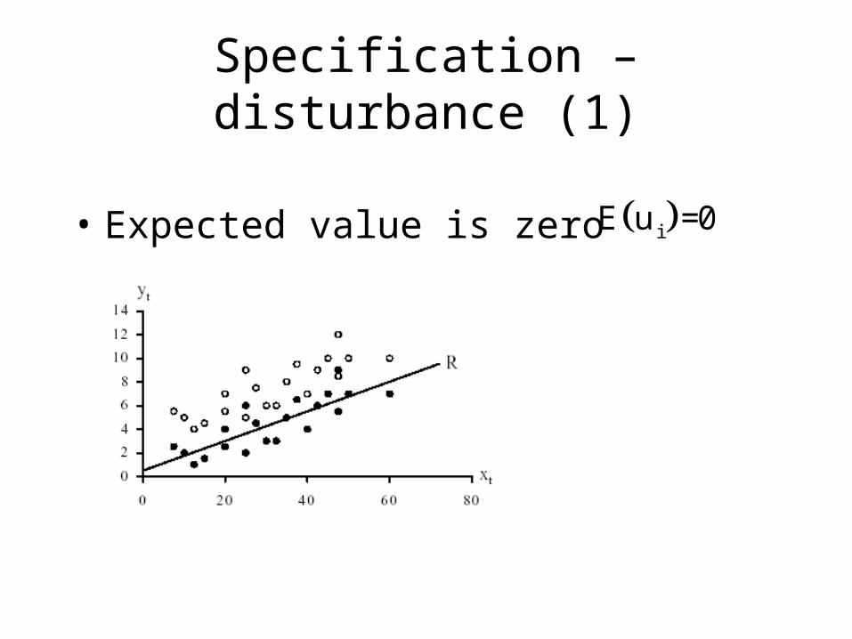
Specification – disturbance (1)

• Expected value is zero iE u =0

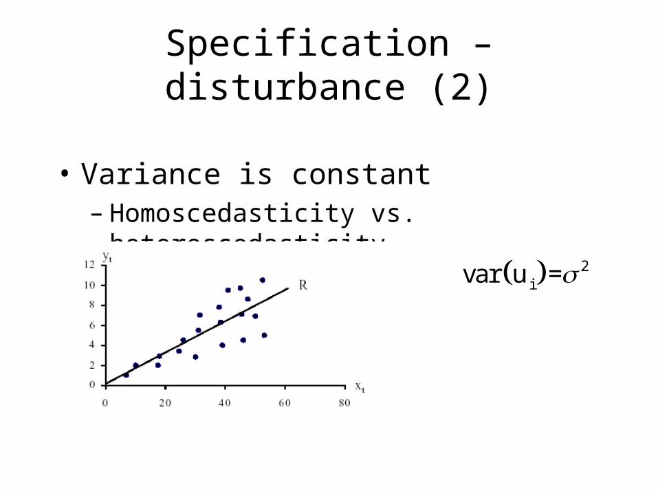
Specification – disturbance (2)

• Variance is constant– Homoscedasticity vs.

heteroscedasticity 2

ivar u =

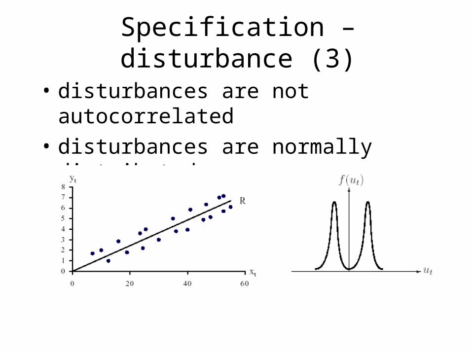
Specification – disturbance (3)

• disturbances are not autocorrelated

• disturbances are normally distributed

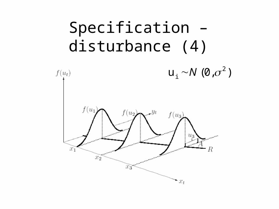
Specification – disturbance (4)

2 iu (0, )N

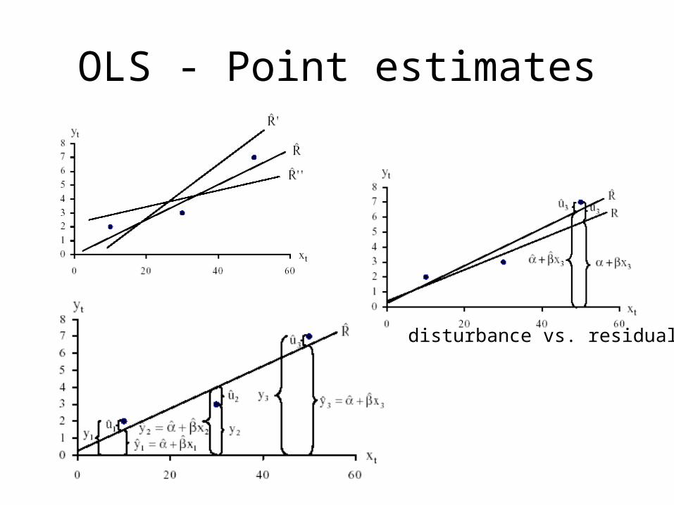
OLS - Point estimates

disturbance vs. residual

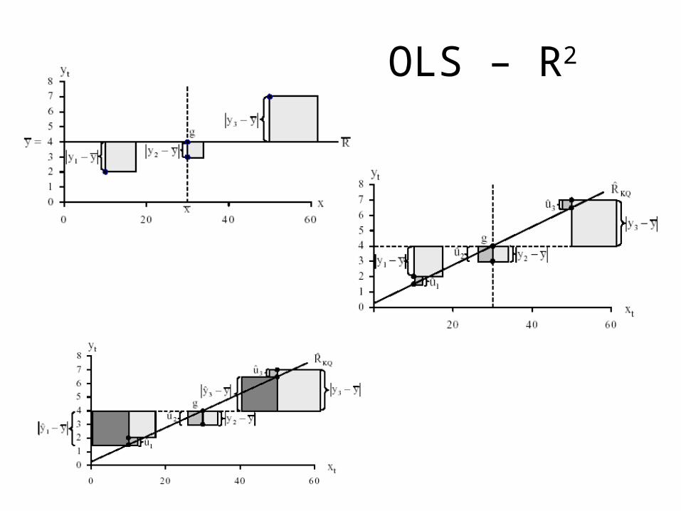
OLS – R2

OLS – hypotheses testing

• T-test

• F-Test

• P values

0 1 2: 0H

0 1: 0H

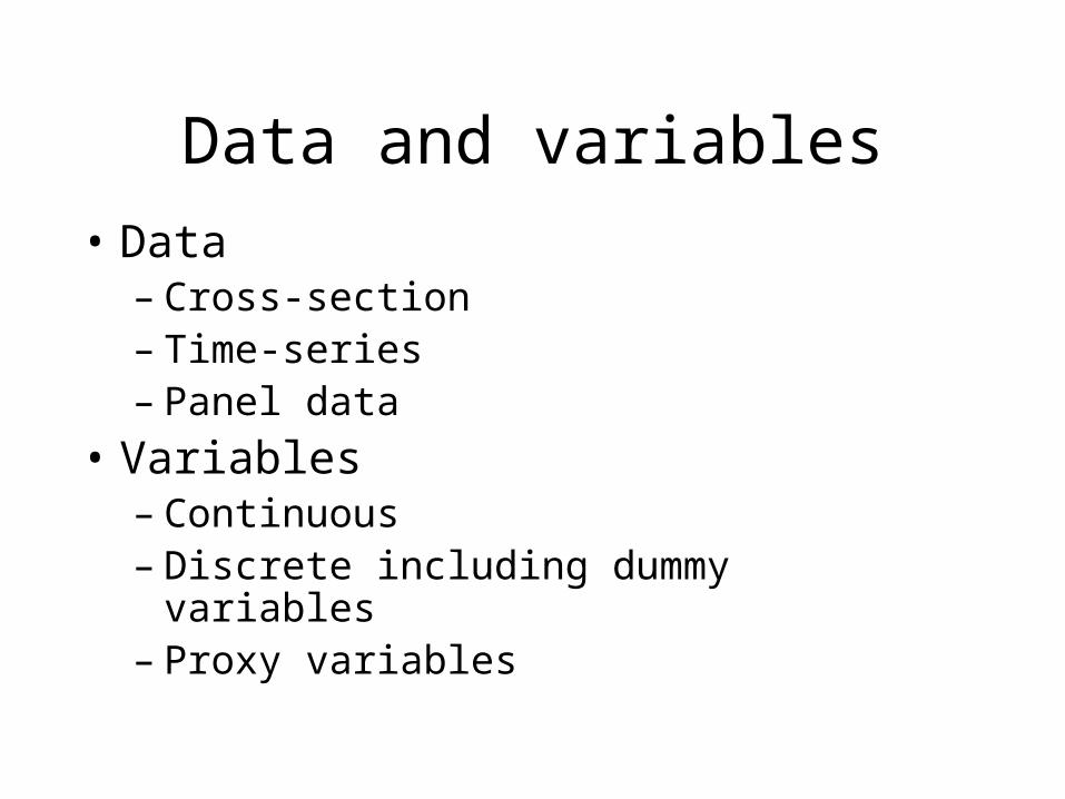
Data and variables• Data

– Cross-section– Time-series– Panel data

• Variables– Continuous– Discrete including dummy variables– Proxy variables

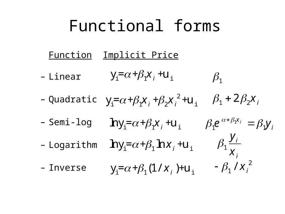
Functional forms

Function Implicit Price

– Linear

– Quadratic

– Semi-log

– Logarithm

– Inverse

i i1lny= + +uix

i i1y= + (1/ )+uix

i i1lny= + ln +uix

i i1y= + +uix 1

21/ ix

11 1

ixie y

1i

i

yx

2i i1 2y= + + +ui ix x 1 22 ix

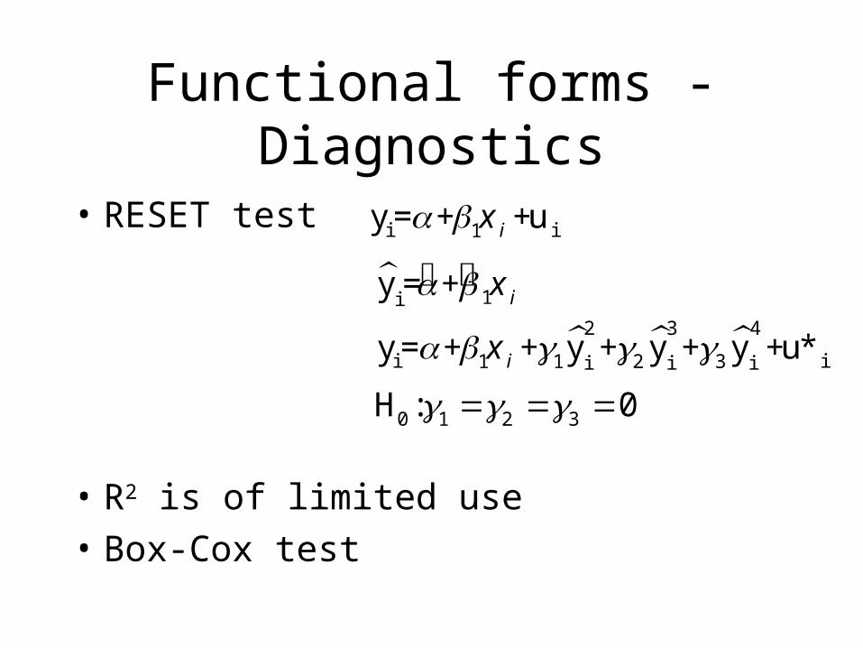
Functional forms - Diagnostics

• RESET test

• R2 is of limited use• Box-Cox test

i i1y= + +uix

1iy = + ix

2 3 4

i i1 1 2 3i i iy= + + y + y + y +u*ix

0 1 2 3H : 0

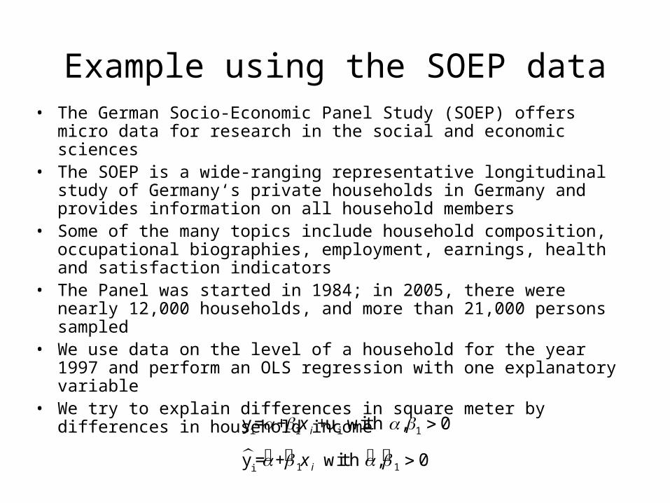
Example using the SOEP data• The German Socio-Economic Panel Study (SOEP) offers

micro data for research in the social and economic sciences • The SOEP is a wide-ranging representative longitudinal

study of Germany‘s private households in Germany and provides information on all household members

• Some of the many topics include household composition, occupational biographies, employment, earnings, health and satisfaction indicators

• The Panel was started in 1984; in 2005, there were nearly 12,000 households, and more than 21,000 persons sampled

• We use data on the level of a household for the year 1997 and perform an OLS regression with one explanatory variable

• We try to explain differences in square meter by differences in household income

1 1iy = + with , 0ix

i i1 1y= + +u with , 0ix

Example results

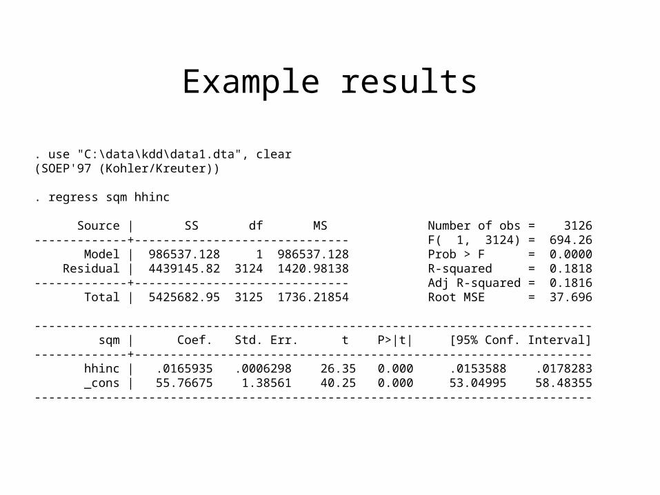
. use "C:\data\kdd\data1.dta", clear(SOEP'97 (Kohler/Kreuter)) . regress sqm hhinc  Source | SS df MS Number of obs = 3126-------------+------------------------------ F( 1, 3124) = 694.26 Model | 986537.128 1 986537.128 Prob > F = 0.0000 Residual | 4439145.82 3124 1420.98138 R-squared = 0.1818-------------+------------------------------ Adj R-squared = 0.1816 Total | 5425682.95 3125 1736.21854 Root MSE = 37.696 ------------------------------------------------------------------------------ sqm | Coef. Std. Err. t P>|t| [95% Conf. Interval]-------------+---------------------------------------------------------------- hhinc | .0165935 .0006298 26.35 0.000 .0153588 .0178283 _cons | 55.76675 1.38561 40.25 0.000 53.04995 58.48355------------------------------------------------------------------------------ 

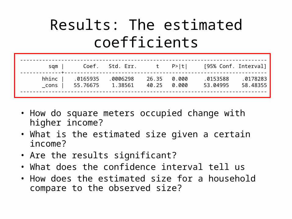
Results: The estimated coefficients

• How do square meters occupied change with higher income?

• What is the estimated size given a certain income?• Are the results significant?• What does the confidence interval tell us• How does the estimated size for a household

compare to the observed size?

 ------------------------------------------------------------------------------ sqm | Coef. Std. Err. t P>|t| [95% Conf. Interval]-------------+---------------------------------------------------------------- hhinc | .0165935 .0006298 26.35 0.000 .0153588 .0178283 _cons | 55.76675 1.38561 40.25 0.000 53.04995 58.48355------------------------------------------------------------------------------ 

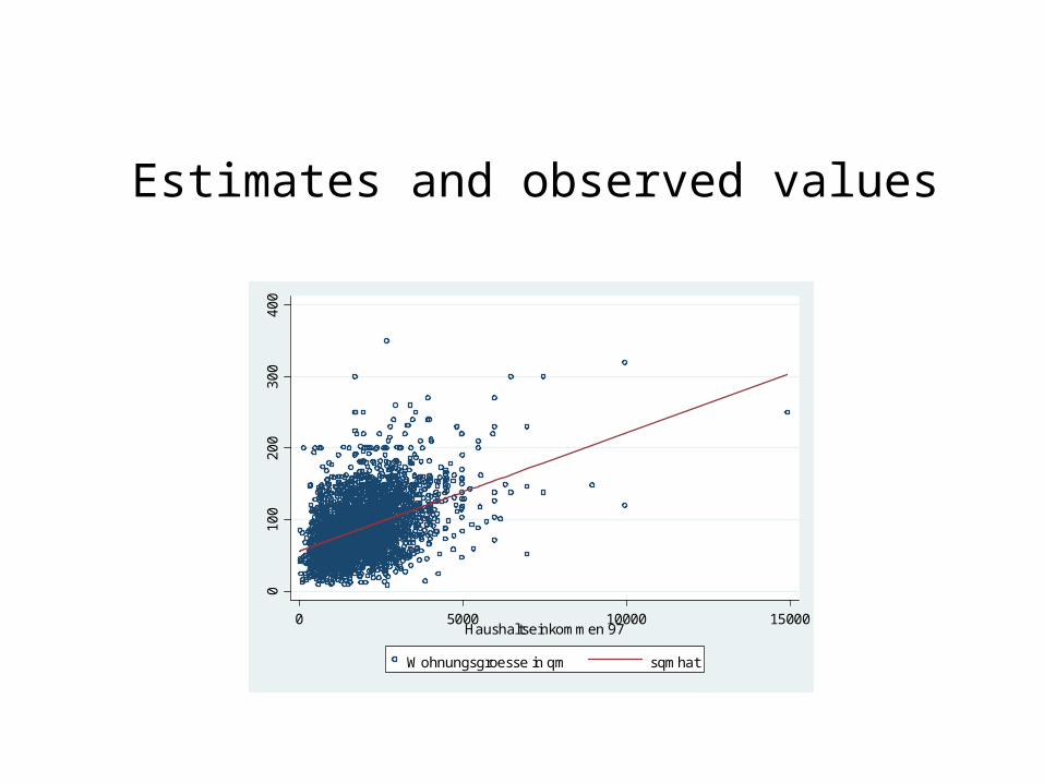
Estimates and observed values

010

020

030

040

0

0 5000 10000 15000Haushaltseinkommen 97

Wohnungsgroesse in qm sqmhat

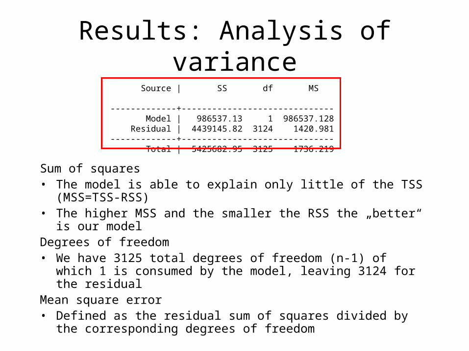
Results: Analysis of variance

Sum of squares• The model is able to explain only little of the TSS

(MSS=TSS-RSS)• The higher MSS and the smaller the RSS the „better“ is

our modelDegrees of freedom• We have 3125 total degrees of freedom (n-1) of which 1

is consumed by the model, leaving 3124 for the residualMean square error• Defined as the residual sum of squares divided by the

corresponding degrees of freedom

  Source | SS df MS -------------+------------------------------ Model | 986537.13 1 986537.128 Residual | 4439145.82 3124 1420.981-------------+------------------------------ Total | 5425682.95 3125 1736.219 

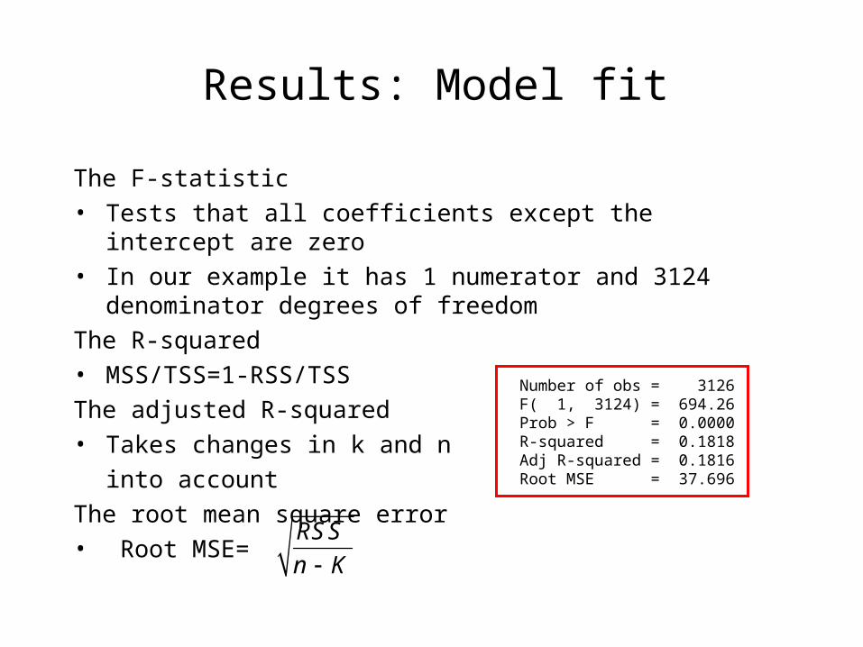
Results: Model fit

The F-statistic • Tests that all coefficients except the intercept are zero• In our example it has 1 numerator and 3124

denominator degrees of freedomThe R-squared• MSS/TSS=1-RSS/TSSThe adjusted R-squared• Takes changes in k and n

into accountThe root mean square error• Root MSE=

 Number of obs = 3126F( 1, 3124) = 694.26Prob > F = 0.0000R-squared = 0.1818Adj R-squared = 0.1816Root MSE = 37.696  

RSSn K

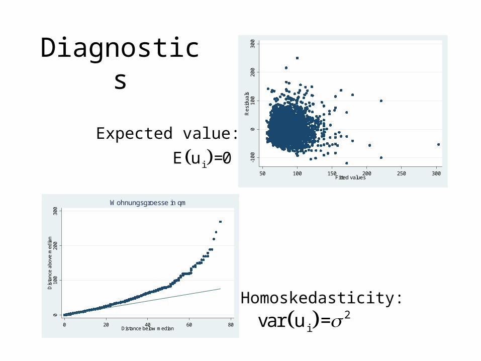
Diagnostics0

100

200

300

Dis

tanc

e a

bove

med

ian

0 20 40 60 80Distance below median

Wohnungsgroesse in qm

2 ivar u =

iE u =0 -10

00

100

200

300

Re

sid

uals

50 100 150 200 250 300Fitted values

Homoskedasticity:

Expected value:

Diagnostics - 2

. hettest

Breusch-Pagan / Cook-Weisberg test for heteroskedasticity

Ho: Constant variance

Variables: fitted values of sqm

chi2(1) = 119.04

Prob > chi2 = 0.0000

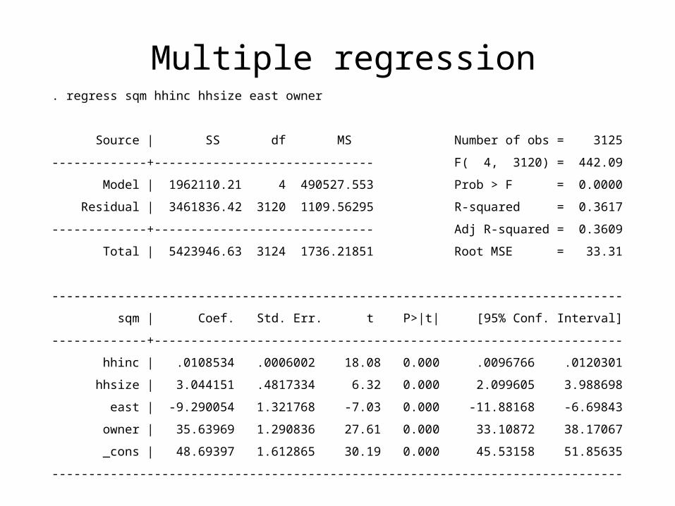
Multiple regression. regress sqm hhinc hhsize east owner

Source | SS df MS Number of obs = 3125

-------------+------------------------------ F( 4, 3120) = 442.09

Model | 1962110.21 4 490527.553 Prob > F = 0.0000

Residual | 3461836.42 3120 1109.56295 R-squared = 0.3617

-------------+------------------------------ Adj R-squared = 0.3609

Total | 5423946.63 3124 1736.21851 Root MSE = 33.31

------------------------------------------------------------------------------

sqm | Coef. Std. Err. t P>|t| [95% Conf. Interval]

-------------+----------------------------------------------------------------

hhinc | .0108534 .0006002 18.08 0.000 .0096766 .0120301

hhsize | 3.044151 .4817334 6.32 0.000 2.099605 3.988698

east | -9.290054 1.321768 -7.03 0.000 -11.88168 -6.69843

owner | 35.63969 1.290836 27.61 0.000 33.10872 38.17067

_cons | 48.69397 1.612865 30.19 0.000 45.53158 51.85635

------------------------------------------------------------------------------