validation of a numerical reservoir model of sedimentary ... · pdf filecho, augustine and...

PROCEEDINGS, Fortieth Workshop on Geothermal Reservoir Engineering

Stanford University, Stanford, California, January 26-28, 2015

SGP-TR-204

1

Validation of a Numerical Reservoir Model of Sedimentary Geothermal Systems Using

Analytical Models

JaeKyoung Cho1, Chad Augustine

2 and Luis E. Zerpa

1

1 Petroleum Engineering Department, Colorado School of Mines, Golden, CO, USA

2 National Renewable Energy Laboratory, Golden, CO, USA

[email protected], [email protected], [email protected]

Keywords: sedimentary geothermal, numerical modeling, validation, well doublet, reservoir modeling.

ABSTRACT

The commercial production of geothermal energy from sedimentary rock formations with relatively low permeability could expand the

current geothermal energy resources toward new regions in the U.S. The feasibility of commercial geothermal production from

sedimentary reservoirs can be studied using numerical reservoir modeling, which allows studying different well configurations and

productivity enhancement techniques. In this paper we present the validation of a numerical reservoir model with respect to an

analytical model, and the process followed to achieve an acceptable match between the numerical and analytical solutions. The

analytical model used is based on the work of Gringarten (1978), which consists of a conceptual sedimentary geothermal reservoir

model, considering an injection and production well doublet in a homogeneous reservoir. The numerical modeling is conducted using a

commercial thermal reservoir simulator. In order to reproduce the analytical model results, the numerical simulation model is modified

to include the same assumptions of the analytical model. The following model parameters are considered to obtain an acceptable match

between the numerical and analytical solutions: grid block size, time step and reservoir areal dimensions; the latter related to boundary

effects on the numerical solution. Here we present lessons learnt and guidelines to improve the numerical simulation solutions. The

agreement between the numerical and analytical models allows us to proceed with confidence to study reservoir enhancement

techniques using numerical reservoir simulation. The validated numerical reservoir model is used to compare the performance of the

geothermal system with and without enhancement treatments (e.g., hydraulic fracturing).

1. INTRODUCTION

Sedimentary enhanced geothermal systems (SEGS) represent a great potential as an energy resource. Unlike conventional convection-

dominated high-enthalpy systems, SEGS are not limited to volcanic or tectonic areas that are less extensive than sedimentary basins in

their areal dimension (Bundschuh and Suarez, 2010). In a report led by the Massachusetts Institute of Technology, it was estimated that

the US could extract 200,000×1018 Joules out of an EGS total potential of 13,000,000×1018 Joules for energy utilization (Tester et al.,

2006).

Sedimentary formations with high temperature at depths ranging from 2 to 6 km can be potential candidates for commercial enhanced

geothermal energy production. The permeability of economically viable potential target formations at such depths is expected to be in

the range of 1 md to 100 md. There is a wide range of variation in petrophysical properties depending on geologic settings. In low

permeability formations (<10 md), fluid flow does not occur naturally at the required flow rates. In this case, reservoir enhancement

techniques can be used for the creation of a reservoir, allowing the access to a huge amount of dormant energy.

Allis et al. (2011) presented a discussion on the potential of geothermal systems in stratigraphic reservoirs of the Western US at depths

of 3 to 5 km. They presented permeability data obtained from oil and gas activity, of the Rocky Mountains and Great Basin of the US.

They showed that a lower Paleozoic carbonate section has permeability up to 70 md, while siliciclastic reservoirs have an average

permeability of 30 md, both at depths of 3 to 5 km. This implies that such carbonate reservoirs with an average permeability of 70 md

could be developed with higher thermal recovery without reservoir enhancement. Moreover, it is suggested that more thermal energy

could be produced from the stratigraphic carbonate reservoir since the heat sweep efficiency is higher than in siliclastic reservoirs,

because of the greater carbonate heat capacity.

Gringarten and Sauty (1975) derived a mathematical model for predicting thermal behavior at the production well for an idealized

geothermal doublet (one injection well and one production well). The mathematical formulation is derived from the partial differential

equation of heat conduction in solids. Under a potential flow theory, they applied the heat conduction equation to a flow channel

bounded by two streamlines. Their formulation assumes constant fluid properties including viscosity, compressibility and the product of

density and heat capacity; an idealized reservoir of laterally infinite geometry with a constant thickness; instantaneous thermal

equilibrium between the rock and water; and no thermal conduction in the horizontal direction and infinite thermal conduction in the

vertical direction. The solution can be used as a design criterion for a geothermal system development, using the temperature behavior at

production well to measure the overall system performance. Satman (2011) investigated the sustainability of geothermal doublets in a

confined aquifer with no natural hydrothermal convection. He presented a field application study of the Lund geothermal heat pump

project based on the work done by Bjelm and Alm (2010). The field application shows that the temperature decline at the producer

follows the Gringarten and Sauty (1975) model. For more complex well configuration, it can be used as a benchmark against which the

performance of other types of well configurations is compared.

Cho, Augustine and Zerpa

2

Deo et al. (2013) discussed thermal performance of sedimentary EGS using reservoir simulation. Five different simulation models were

considered: sandwich, single layer, low temperature, low permeability and short circuit model. Interestingly, the lower permeability

model shows the best thermal performance because there is less permeability difference between the cap/bed rock and reservoir,

facilitating heat transfer from the sealing units. This implies that there are two conflicting processes: thermal and hydraulic performance.

Therefore, balancing thermal and hydraulic performance is the most crucial element for successful sedimentary EGS.

In this paper we present the comparison of a numerical reservoir model with respect to an analytical model, and the process followed to

achieve an acceptable match between the numerical and analytical solutions. The analytical model used is based on the work of

Gringarten (1978), which consists of a conceptual sedimentary geothermal reservoir model, considering an injection and production

well doublet in a homogeneous reservoir. The numerical modeling is conducted using a commercial thermal reservoir simulator. In

order to reproduce the analytical model results, the numerical simulation model is modified to include the same assumptions of the

analytical model. The following model parameters are considered to obtain an acceptable match between the numerical and analytical

solutions: grid block size, time step and reservoir areal dimensions; the latter related to boundary effects on the numerical solution. Here

we present lessons learnt and guidelines to improve the numerical simulation solutions. The agreement between the numerical and

analytical models allows us to proceed with confidence to study reservoir enhancement techniques using numerical reservoir simulation.

Using the reservoir model developed, we studied different reservoir enhancement techniques. Four different reservoir enhancement

techniques are considered in this study: i) vertical well doublet with hydraulic fractures; ii) horizontal wells with open-hole completions;

iii) horizontal wells with longitudinal hydraulic fractures; and iv) horizontal wells with multi-stage hydraulic fractures. These reservoir

enhancement techniques are compared to a base case, which consists of an injection and production well doublet. The performance of

the different scenarios considered is evaluated in terms of the hydraulic behavior (i.e., well productivity/injectivity), and thermal

evolution of the reservoir (i.e., thermal breakthrough time). We found that the reservoir hydraulic behavior is improved by the use of

hydraulic fractures, while the thermal breakthrough time is increased by the introduction of reservoir enhancement techniques.

2. ANALYTICAL MODELING OF SEDIMENTARY GEOTHERMAL SYSTEMS

A conceptual sedimentary geothermal reservoir, consisting of an injection and production well doublet in a homogenous porous media,

is considered (Figure 1). Sedimentary geothermal reservoir performance is described by two factors: the thermal performance of the

reservoir (the time for thermal breakthrough at the production well), and the pressure profile in the reservoir (the pressure drive required

to maintain a desired flow rate between the injection and production wells). Gringarten (1978) describes simple analytical models for

both of these factors.

Figure 1: Geothermal doublet system.

The assumptions made in the derivation of Gringarten’s analytical model are:

Horizontal aquifer with uniform thickness.

Sealed aquifer by cap/bed rocks.

Constant injection rate equal to production rate (i.e., steady-state condition).

Initially, rock and fluid are in thermal equilibrium at same temperature.

Horizontal heat conduction is neglected.

Vertical heat conduction from cap/bed rock is considered.

Volumetric heat capacity of water and rock are constant.

The time for thermal breakthrough in the reservoir (i.e., for the temperature of the produced fluid to drop below the initial reservoir

temperature, To) is defined as the lifetime of the well doublet, t, and is described by Eq. (12) in Gringarten (1978):

Dt = f + 1-f( )rrCrrwCw

é

ëê

ù

ûúp

3

D2h

Q (1)

where D is the distance between wells in m, Q is the volumetric injection/production well flow rate (m3/s), h is the reservoir thickness

(m), is the reservoir porosity, ρwCw is the water heat capacity (kJ/m3/ºC), and ρrCr is the rock heat capacity (kJ/m3/ºC).


3

The pressure drive between the wells in the reservoir, Δp, (or more accurately, the difference between the injection and production well

pressure), is described by Gringarten (1978), Eq. (13)) as the pressure drawdown in the production well. Muskat (1946) describes how

to relate the pressure difference between the wells. The result is:

Dp =mQ

pkhln

D

rwell

æ

èç

ö

ø÷ (2)

where p is the pressure difference between injection and production wells, k is the reservoir permeability, is the water viscosity, and

rwell is the well radius.

Table 1 shows the values of the rock and fluid properties used as base case for the comparison between the analytical and numerical

model results of a sedimentary geothermal reservoir.

Table 1: Rock and fluid properties used in base case for comparison between analytical and numerical models.

Parameter Value

Porosity, 0.15

Reservoir thickness, h 50 m

Rock heat capacity, rCp,r 2,770 kJ/m3/oC

Water heat capacity, wCp,w 3,860 kJ/m3/oC

Water viscosity, avg 2.18e-4 Pa-s

Well radius, rwell 0.108 m (8.5” diam.)

Reservoir lifetime, t 30 years

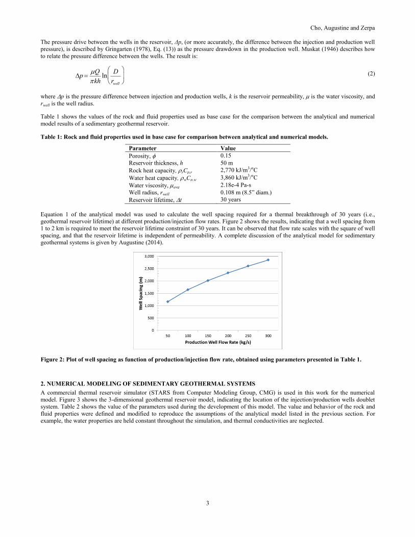
Equation 1 of the analytical model was used to calculate the well spacing required for a thermal breakthrough of 30 years (i.e.,

geothermal reservoir lifetime) at different production/injection flow rates. Figure 2 shows the results, indicating that a well spacing from

1 to 2 km is required to meet the reservoir lifetime constraint of 30 years. It can be observed that flow rate scales with the square of well

spacing, and that the reservoir lifetime is independent of permeability. A complete discussion of the analytical model for sedimentary

geothermal systems is given by Augustine (2014).

Figure 2: Plot of well spacing as function of production/injection flow rate, obtained using parameters presented in Table 1.

2. NUMERICAL MODELING OF SEDIMENTARY GEOTHERMAL SYSTEMS

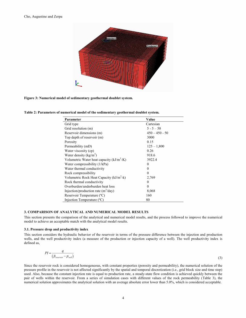
A commercial thermal reservoir simulator (STARS from Computer Modeling Group, CMG) is used in this work for the numerical

model. Figure 3 shows the 3-dimensional geothermal reservoir model, indicating the location of the injection/production wells doublet

system. Table 2 shows the value of the parameters used during the development of this model. The value and behavior of the rock and

fluid properties were defined and modified to reproduce the assumptions of the analytical model listed in the previous section. For

example, the water properties are held constant throughout the simulation, and thermal conductivities are neglected.


4

Figure 3: Numerical model of sedimentary geothermal doublet system.

Table 2: Parameters of numerical model of the sedimentary geothermal doublet system.

Parameter Value

Grid type Cartesian

Grid resolution (m) 5 - 5 – 50

Reservoir dimensions (m) 450 – 450 - 50

Top depth of reservoir (m) 3000

Porosity 0.15

Permeability (mD) 125 – 1,800

Water viscosity (cp) 0.26

Water density (kg/m3) 918.6

Volumetric Water heat capacity (kJ/m3-K) 3922.4

Water compressibility (1/kPa) 0

Water thermal conductivity 0

Rock compressibility 0

Volumetric Rock Heat Capacity (kJ/m3-k) 2,769

Rock thermal conductivity 0

Overburden/underburden heat loss 0

Injection/production rate (m3/day) 8,068

Reservoir Temperature (ºC) 160

Injection Temperature (ºC) 80

3. COMPARISON OF ANALYTICAL AND NUMERICAL MODEL RESULTS

This section presents the comparison of the analytical and numerical model results, and the process followed to improve the numerical

model to achieve an acceptable match with the analytical model results.

3.1. Pressure drop and productivity index

This section considers the hydraulic behavior of the reservoir in terms of the pressure difference between the injection and production

wells, and the well productivity index (a measure of the production or injection capacity of a well). The well productivity index is

defined as,

PI =q

preservoir - pwell( ) (3)

Since the reservoir rock is considered homogeneous, with constant properties (porosity and permeability), the numerical solution of the

pressure profile in the reservoir is not affected significantly by the spatial and temporal discretization (i.e., grid block size and time step)

used. Also, because the constant injection rate is equal to production rate, a steady-state flow condition is achieved quickly between the

pair of wells within the reservoir. From a series of simulation cases with different values of the rock permeability (Table 3), the

numerical solution approximates the analytical solution with an average absolute error lower than 5.0%, which is considered acceptable.


5

Table 3: Pressure difference between injector and producer, and productivity index, obtained with the analytical and numerical

models.

Permeability (mD) 125 200 300 600 1,800 Abs. relative

error (%)

P (kPa)

Analytic 11,785 7,365 4,910 2,455 818

4.75 %

Numerical 12,344 7,715 5,143 2,571 857

Productivity

Index, PI

(L/s-bar)

Analytic 1.58 2.54 3.80 7.61 22.82

3.90 %

Numerical 1.52 2.44 3.65 7.31 21.92

3.2. Effect of numerical grid size on thermal breakthrough time

When considering the thermal behavior of the reservoir, the scenario is different than the hydraulic behavior. Since cold water is

injected into a hot reservoir to displace hot fluids towards the production well, the system is constantly under unsteady-state conditions.

The thermal evolution of the reservoir, obtained with the numerical model, is affected by the spatial discretization or grid block sizes

because of the magnitude of numerical dispersion. Figure 4 shows the temperature change with time at the location of the production

well obtained with different grid block sizes. The typical behavior of temperature as a function of time observed in each solution

presents a constant temperature equal to the initial reservoir temperature, followed by a decline in temperature because of arrival of

colder water to the production well. The time when the temperature begins to decrease is known as the thermal breakthrough time. After

this time the temperature at the location of the production well decreases constantly.

Figure 4: Plot of temperature at the production well location as function of time, showing effect of model grid block size (in

meters) on calculated thermal breakthrough time.

The numerical solution obtained changes with the grid block size used in the reservoir model. The case with the coarser grid (100 x

100 m) presents an earlier thermal breakthrough time and a lower temperature decline rate, while the case with the finer grid (2.5 x

2.5 m) presents a longer thermal breakthrough time with a sharper thermal front arriving to the production well. A higher temperature

decline rate corresponds to a sharper thermal front, which indicates lower numerical dispersion. Table 4 summarizes the numerical

results obtained with different grid block sizes and presents a comparison with the analytical solution. The thermal breakthrough time

increases with decreasing grid block size, and the relative error between the numerical and analytical solution decreases with decreasing

grid block size. At this point, the relative error is too high (> 10%) to be considered acceptable.

Table 4: Summary of numerical results of thermal breakthrough time obtained with different grid block sizes, and comparison

with analytical solution.

Grid block

size (m)

Reservoir size

(m)

Well spacing

(m)

Thermal breakthrough time

Relative error (%) Analytical

solution

Numerical

solution

100 x 100 4,500 x 3,000 1,500 30.0 16.0 46.7

50 x 50 4,500 x 3,000 1,500 30.0 19.0 36.6

10 x 10 4,500 x 3,000 1,500 30.0 22.0 26.6

5 x 5 4,500 x 3,000 1,500 30.0 23.0 23.3

2.5 x 2.5 4,500 x 3,000 1,500 30.0 24.0 20.0

0 10 20 30 40135

140

145

150

155

160

Time (yr)

Tem

pera

ture

(ºC

)

100 100

50 50

10 10

5 5

2.5 2.5


6

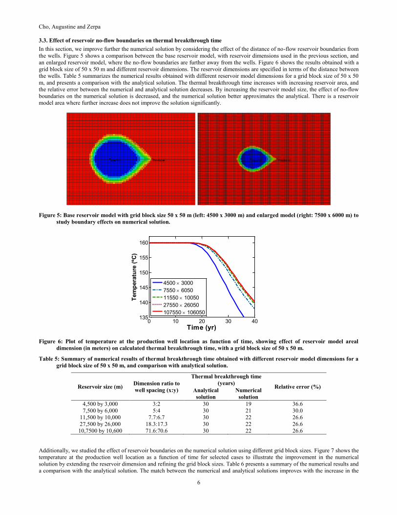
3.3. Effect of reservoir no-flow boundaries on thermal breakthrough time

In this section, we improve further the numerical solution by considering the effect of the distance of no-flow reservoir boundaries from

the wells. Figure 5 shows a comparison between the base reservoir model, with reservoir dimensions used in the previous section, and

an enlarged reservoir model, where the no-flow boundaries are further away from the wells. Figure 6 shows the results obtained with a

grid block size of 50 x 50 m and different reservoir dimensions. The reservoir dimensions are specified in terms of the distance between

the wells. Table 5 summarizes the numerical results obtained with different reservoir model dimensions for a grid block size of 50 x 50

m, and presents a comparison with the analytical solution. The thermal breakthrough time increases with increasing reservoir area, and

the relative error between the numerical and analytical solution decreases. By increasing the reservoir model size, the effect of no-flow

boundaries on the numerical solution is decreased, and the numerical solution better approximates the analytical. There is a reservoir

model area where further increase does not improve the solution significantly.

Figure 5: Base reservoir model with grid block size 50 x 50 m (left: 4500 x 3000 m) and enlarged model (right: 7500 x 6000 m) to

study boundary effects on numerical solution.

Figure 6: Plot of temperature at the production well location as function of time, showing effect of reservoir model areal

dimension (in meters) on calculated thermal breakthrough time, with a grid block size of 50 x 50 m.

Table 5: Summary of numerical results of thermal breakthrough time obtained with different reservoir model dimensions for a

grid block size of 50 x 50 m, and comparison with analytical solution.

Reservoir size (m) Dimension ratio to

well spacing (x:y)


(years) Relative error (%)

Analytical

solution

Numerical

solution

4,500 by 3,000 3:2 30 19 36.6

7,500 by 6,000 5:4 30 21 30.0

11,500 by 10,000 7.7:6.7 30 22 26.6

27,500 by 26,000 18.3:17.3 30 22 26.6

10,7500 by 10,600 71.6:70.6 30 22 26.6

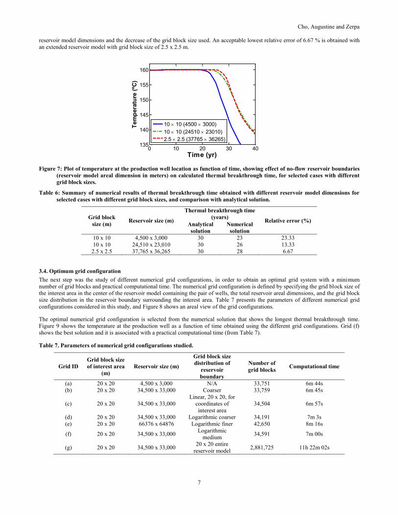
Additionally, we studied the effect of reservoir boundaries on the numerical solution using different grid block sizes. Figure 7 shows the

temperature at the production well location as a function of time for selected cases to illustrate the improvement in the numerical

solution by extending the reservoir dimension and refining the grid block sizes. Table 6 presents a summary of the numerical results and

a comparison with the analytical solution. The match between the numerical and analytical solutions improves with the increase in the

0 10 20 30 40135

140

145

150

155

160

Time (yr)

Tem

pera

ture

(ºC

)

4500 3000

7550 6050

11550 10050

27550 26050

107550 106050


7

reservoir model dimensions and the decrease of the grid block size used. An acceptable lowest relative error of 6.67 % is obtained with

an extended reservoir model with grid block size of 2.5 x 2.5 m.

Figure 7: Plot of temperature at the production well location as function of time, showing effect of no-flow reservoir boundaries

(reservoir model areal dimension in meters) on calculated thermal breakthrough time, for selected cases with different

grid block sizes.

Table 6: Summary of numerical results of thermal breakthrough time obtained with different reservoir model dimensions for

selected cases with different grid block sizes, and comparison with analytical solution.

Grid block

size (m) Reservoir size (m)


(years) Relative error (%)

Analytical

solution

Numerical

solution

10 x 10 4,500 x 3,000 30 23 23.33

10 x 10 24,510 x 23,010 30 26 13.33

2.5 x 2.5 37,765 x 36,265 30 28 6.67

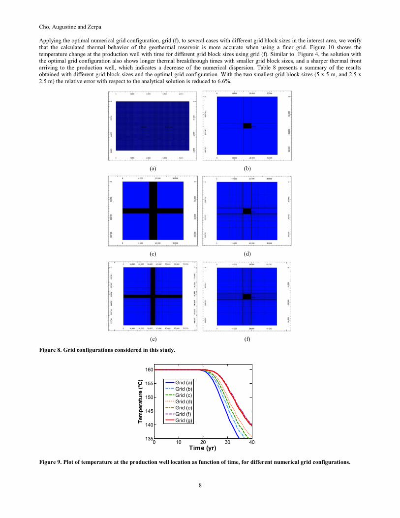
3.4. Optimum grid configuration

The next step was the study of different numerical grid configurations, in order to obtain an optimal grid system with a minimum

number of grid blocks and practical computational time. The numerical grid configuration is defined by specifying the grid block size of

the interest area in the center of the reservoir model containing the pair of wells, the total reservoir areal dimensions, and the grid block

size distribution in the reservoir boundary surrounding the interest area. Table 7 presents the parameters of different numerical grid

configurations considered in this study, and Figure 8 shows an areal view of the grid configurations.

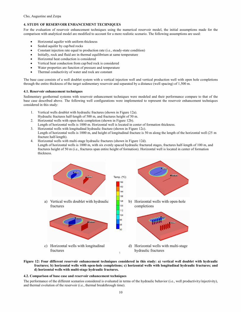
The optimal numerical grid configuration is selected from the numerical solution that shows the longest thermal breakthrough time.

Figure 9 shows the temperature at the production well as a function of time obtained using the different grid configurations. Grid (f)

shows the best solution and it is associated with a practical computational time (from Table 7).

Table 7. Parameters of numerical grid configurations studied.

Grid ID

Grid block size

of interest area

(m)

Reservoir size (m)

Grid block size

distribution of

reservoir

boundary

Number of

grid blocks Computational time

(a) 20 x 20 4,500 x 3,000 N/A 33,751 6m 44s

(b) 20 x 20 34,500 x 33,000 Coarser 33,759 6m 45s

(c) 20 x 20 34,500 x 33,000

Linear, 20 x 20, for

coordinates of

interest area

34,504 6m 57s

(d) 20 x 20 34,500 x 33,000 Logarithmic coarser 34,191 7m 3s

(e) 20 x 20 66376 x 64876 Logarithmic finer 42,650 8m 16s

(f) 20 x 20 34,500 x 33,000 Logarithmic

medium 34,591 7m 00s

(g) 20 x 20 34,500 x 33,000 20 x 20 entire

reservoir model 2,881,725 11h 22m 02s

0 10 20 30 40135

140

145

150

155

160

Time (yr)

Tem

pera

ture

(ºC

)

10 10 (4500 3000)

10 10 (24510 23010)

2.5 2.5 (37765 36265)


8

Applying the optimal numerical grid configuration, grid (f), to several cases with different grid block sizes in the interest area, we verify

that the calculated thermal behavior of the geothermal reservoir is more accurate when using a finer grid. Figure 10 shows the

temperature change at the production well with time for different grid block sizes using grid (f). Similar to Figure 4, the solution with

the optimal grid configuration also shows longer thermal breakthrough times with smaller grid block sizes, and a sharper thermal front

arriving to the production well, which indicates a decrease of the numerical dispersion. Table 8 presents a summary of the results

obtained with different grid block sizes and the optimal grid configuration. With the two smallest grid block sizes (5 x 5 m, and 2.5 x

2.5 m) the relative error with respect to the analytical solution is reduced to 6.6%.

(a) (b)

(c) (d)

(e) (f)

Figure 8. Grid configurations considered in this study.

Figure 9. Plot of temperature at the production well location as function of time, for different numerical grid configurations.

0 10 20 30 40135

140

145

150

155

160

Time (yr)

Tem

pera

ture

(ºC

)

Grid (a)

Grid (b)

Grid (c)

Grid (d)

Grid (e)

Grid (f)

Grid (g)


9

Figure 10. Plot of temperature at the production well location as function of time, for different grid block sizes using grid

configuration (f).

Table 8. Summary of numerical results of thermal breakthrough time obtained with different grid block sizes using grid (f), and

comparison with analytical solution.

Grid block

size (m) Reservoir size (m)

Well

spacing (m)

Thermal breakthrough time Relative error

(%) Analytical

solution

Numerical

solution

100 x 100 34,500 x 33,000 1,500 30 19 36.6%

50 x 50 34,500 x 33,000 1,500 30 22 26.6%

20 x 20 34,500 x 33,000 1,500 30 25 16.6%

10 x 10 34,500 x 33,000 1,500 30 27 10.0%

5 x 5 34,500 x 33,000 1,500 30 28 6.6%

2 x 2 34,500 x 33,000 1,500 30 28 6.6%

3.5. Time step effect

We perform an evaluation of the time step used during the numerical solution of the flow and thermal behavior of the geothermal

reservoir, which also plays a role in the accuracy of the solution by affecting the numerical dispersion. Figure 11 shows the temperature

change at the production well with time obtained using different time step values for a grid block size of 10 x 10 m. For time steps less

than 1 month the change in the solution is not significant, which indicates that a time step of 1 month is an appropriate value for the

maximum time step to be used in the simulation.

Figure 11. Plot of temperature at the production well location as function of time, for different time steps used during the

numerical simulation with a grid block size of 10 x 10 m.

0 10 20 30 40135

140

145

150

155

160

Time (yr)T

em

pera

ture

(ºC

)

100 100

50 50

20 20

10 10

5 5

2 2

0 10 20 30 40135

140

145

150

155

160

Time (yr)

Tem

pera

ture

(ºC

)

T = 10 days

T = 30 days

T = 365 days

T = 1000 days


10

4. STUDY OF RESERVOIR ENHANCEMENT TECHNIQUES

For the evaluation of reservoir enhancement techniques using the numerical reservoir model, the initial assumptions made for the

comparison with analytical model are modified to account for a more realistic scenario. The following assumptions are used:

Horizontal aquifer with uniform thickness

Sealed aquifer by cap/bed rocks

Constant injection rate equal to production rate (i.e., steady-state condition)

Initially, rock and fluid are in thermal equilibrium at same temperature

Horizontal heat conduction is considered

Vertical heat conduction from cap/bed rock is considered

Water properties are function of pressure and temperature

Thermal conductivity of water and rock are constant

The base case consists of a well doublet system with a vertical injection well and vertical production well with open hole completions

through the entire thickness of the target sedimentary reservoir and separated by a distance (well spacing) of 1,500 m.

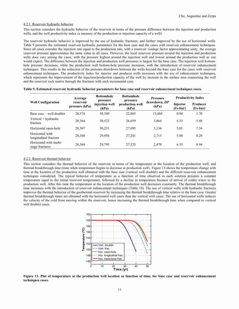
4.1. Reservoir enhancement techniques

Sedimentary geothermal systems with reservoir enhancement techniques were modeled and their performance compare to that of the

base case described above. The following well configurations were implemented to represent the reservoir enhancement techniques

considered in this study:

1. Vertical wells doublet with hydraulic fractures (shown in Figure 12a).

Hydraulic fractures half-length of 500 m, and fractures height of 50 m.

2. Horizontal wells with open-hole completion (shown in Figure 12b).

Length of horizontal wells is 1000 m. Horizontal well is located in center of formation thickness.

3. Horizontal wells with longitudinal hydraulic fracture (shown in Figure 12c).

Length of horizontal wells is 1000 m, and height of longitudinal fracture is 50 m along the length of the horizontal well (25 m

fracture half-length).

4. Horizontal wells with multi-stage hydraulic fractures (shown in Figure 12d).

Length of horizontal wells is 1000 m, with six evenly spaced hydraulic fractured stages, fractures half-length of 100 m, and

fractures height of 50 m (i.e., fractures span entire height of formation). Horizontal well is located in center of formation

thickness.

Figure 12: Four different reservoir enhancement techniques considered in this study: a) vertical well doublet with hydraulic

fractures; b) horizontal wells with open-hole completions; c) horizontal wells with longitudinal hydraulic fractures; and

d) horizontal wells with multi-stage hydraulic fractures.

4.2. Comparison of base case and reservoir enhancement techniques

The performance of the different scenarios considered is evaluated in terms of the hydraulic behavior (i.e., well productivity/injectivity),

and thermal evolution of the reservoir (i.e., thermal breakthrough time).


11

4.2.1. Reservoir hydraulic behavior

This section considers the hydraulic behavior of the reservoir in terms of the pressure difference between the injection and production

wells, and the well productivity index (a measure of the production or injection capacity of a well).

The reservoir hydraulic behavior is improved by the use of hydraulic fractures, and further improved by the use of horizontal wells.

Table 9 presents the estimated reservoir hydraulic parameters for the base case and the cases with reservoir enhancement techniques.

Since all cases consider the injection rate equal to the production rate, with a reservoir voidage factor approximating unity, the average

reservoir pressure approximates the same value in all cases. However, the local reservoir pressure around the injection and production

wells does vary among the cases, with the pressure highest around the injection well and lowest around the production well as one

would expect. The difference between the injection and production well pressures is largest for the base case. The injection well bottom-

hole pressure decreases, while the production well bottom-hole pressure increases, with the introduction of reservoir enhancement

techniques. This results in the reduction of the pressure drawdown between the wells beyond the base case for the cases with reservoir

enhancement techniques. The productivity index for injector and producer wells increases with the use of enhancement techniques,

which represents the improvement of the injection/production capacity of the well by increase in the surface area connecting the well

and the reservoir rock matrix through the fractures with each incremental case.

Table 9. Estimated reservoir hydraulic behavior parameters for base case and reservoir enhancement techniques cases.

Well Configuration

Average

reservoir

pressure (kPa)

Bottomhole

pressure

injection well

(kPa)

Bottomhole

pressure

production well

(kPa)

Pressure

drawdown, DP

(kPa)

Productivity Index

Injector

(l/s-bar)

Producer

(l/s-bar)

Base case – well doublet 28,374 38,349 22,865 15,484 0.94 1.70

Vertical + hydraulic

fracture 28,364 30,523 26,659 3,864 4.33 5.48

Horizontal open-hole 28,367 30,231 27,095 3,136 5.01 7.34

Horizontal with

longitudinal fracture 28,368 29,956 27,241 2,715 5.88 8.29

Horizontal with multi-

stage fractures 28,369 29,795 27,325 2,470 6.55 8.94

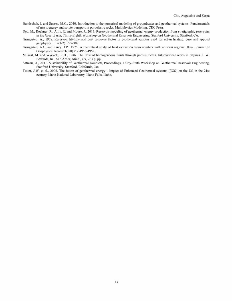
4.2.2. Reservoir thermal behavior

This section considers the thermal behavior of the reservoir in terms of the temperature at the location of the production well, and

thermal breakthrough time (time when temperature begins to decrease at production well). Figure 13 shows the temperature change with

time at the location of the production well obtained with the base case (vertical well doublet) and the different reservoir enhancement

techniques considered. The typical behavior of temperature as a function of time observed in each solution presents a constant

temperature equal to the initial reservoir temperature, followed by a decline in temperature because of arrival of colder water to the

production well. After this time the temperature at the location of the production well decreases constantly. The thermal breakthrough

time increases with the introduction of reservoir enhancement techniques (Table 10). The use of vertical wells with hydraulic fractures

improves the thermal behavior of the geothermal reservoir by increasing the thermal breakthrough time relative to the base case. Greater

thermal breakthrough times are obtained with the horizontal well cases than the vertical well cases. The use of horizontal wells reduces

the velocity of the cold front moving within the reservoir, hence increasing the thermal breakthrough time when compared to vertical

well doublet cases.

Figure 13. Plot of temperature at the production well location as function of time, for base case and reservoir enhancement

techniques cases.

0 10 20 30 40 50

146

148

150

152

154

156

158

160

162

Time (yr)

Tem

pera

ture

(ºC

)

Vert. doublet

Vert. frac.

Hor. open-hole

Hor. longitudinal frac.

Hor. transverse frac.


12

Table 10. Thermal breakthrough time obtained from base case and different reservoir enhancement techniques.

Well Configuration Thermal breakthrough

time (yr)

Base case – well doublet 27

Vertical + hydraulic fracture 36

Horizontal open-hole 40

Horizontal with longitudinal fracture 42

Horizontal with multi-fracture 41

5. CONCLUSIONS

A rigorous study comparing the results of the analytic model for the hydraulic and thermal behavior of flow between a well doublet pair

in a sedimentary reservoir to numerical modeling of the same system showed that the numeric model results for the hydraulic behavior

are insensitive to the grid configuration, but that the model results for thermal behavior can be heavily dependent on grid size, modeled

reservoir area (boundary effects), time step, and grid configuration. Systematic model runs showed that insufficient grid sizing causes

numerical dispersion that causes the numerical model to underestimate the thermal breakthrough time compared to the analytic model.

As grid sizing is decreased, the model results converge on a solution (Figure 4). Likewise, insufficient reservoir model area introduces

boundary effects in the numerical solution that cause the model results to differ from the numerical model. Increasing the reservoir

model area improves the agreement of the numerical model results to the analytical model results by better approximating the “infinite

reservoir” assumption of the analytical model. As reservoir model area increases, the numerical model results converge and the benefits

of using even larger reservoir model areas diminishes (Figure 6).

A numerical model using a small grid size (2.5x2.5 m) and large reservoir model area (37,765m x 36,265m) was found to give

numerical results for the thermal breakthrough time in good agreement with the analytical model (see Table 6 and Figure 7). However,

using small grid sizes and large reservoir model areas results in a large number of grid cells and prohibitive computational times (see

Table 7, case g). Different grid configurations that use a fine grid mesh in the area of interest and a coarse grid mesh in the outer regions

where the temperature and pressure gradients are small were tested to find one that gave an accurate solution in a reasonable amount of

computational time. The resulting optimal grid configuration was found to use a total reservoir model area of 34.5 km x 33 km, a 5x5 m

spacing in the area of interest closest to the well doublet, and a logarithmic medium algorithm to determine grid block size distribution

in areas around the reservoir boundary. This configuration resulted in a computed temperature breakthrough time within 6.6% of the

analytic solution. A numerical simulation using 2x2 m spacing in the area of interest confirmed that additional reductions in grid size

did not significantly change the numerical model results. Finally, a study of the impact of time step found that assuming a one-month

time step gave consistent results.

The study demonstrated that special attention must be paid to the reservoir grid used to ensure that numerical results are accurate and

not overly influenced by numerical dispersion and boundary effects. Trade-offs must be made in terms of the number of grid cells used

in the model and the computational time required. The systematic study of the influence of these factors on numerical model results

compared to an analytic model demonstrated that our numerical model can give accurate results and gave us guidance on the reservoir

model area and grid sizing to use in future numerical modeling.

Four different reservoir enhancement techniques were compared against a base case. The base case consists of a sedimentary

geothermal reservoir with an injection and production well doublet. The performance of the different scenarios considered was

evaluated in terms of the hydraulic behavior (i.e., productivity/injectivity), and thermal evolution of the reservoir (i.e., thermal

breakthrough time). The reservoir enhancement techniques can have a significant impact on geothermal reservoir performance. The

productivity index of injector and producer wells increase by a factor of 5, approximately, with the use of enhancement techniques. This

is due to the augmented surface area connecting the well and the reservoir rock matrix through the fractures in each reservoir

enhancement technique tested. The geothermal reservoir lifetime is increased by 50%, approximately, by the use of horizontal wells

using the same well spacing as the base case (vertical well doublet) and same injection/production rate. The use of horizontal wells

reduces the velocity of the cold front moving within the reservoir, hence increasing the thermal breakthrough time when compared to

vertical well doublet cases. The most promising reservoir enhancement techniques are horizontal wells with longitudinal fracture and

horizontal wells with multi-stage hydraulic fractures.

ACKNOWLEDGEMENTS

This work was supported by the U.S. Department of Energy, Office of Energy Efficiency and Renewable Energy (EERE), Geothermal

Technologies Office (GTO) under Contract No.DE-AC36-08-GO28308 with the National Renewable Energy Laboratory.

REFERENCES

Allis, R. et al., 2011. The potential for basin-centered geothermal resources in the Great Basin. Geothermal Resources Council

Transactions, 35: 683-688.

Augustine, C., 2014. Analysis of sedimentary geothermal systems using an analytical reservoir model. Geothermal Resources Council

Transactions, 38: 641-647.

Bjelm, L. and Alm, P., 2010. Reservoir Cooling After 25 Years of Heat Production in the Lund Geothermal Heat Pump Project,

Proceedings, World Geothermal Congress.


13

Bundschuh, J. and Suarez, M.C., 2010. Introduction to the numerical modeling of groundwater and geothermal systems: Fundamentals

of mass, energy and solute transport in poroelastic rocks. Multiphysics Modeling. CRC Press.

Deo, M., Roehner, R., Allis, R. and Moore, J., 2013. Reservoir modeling of geothermal energy production from stratigraphic reservoirs

in the Great Basin, Thirty-Eighth Workshop on Geothermal Reservoir Engineering. Stanford University, Stanford, CA.

Gringarten, A., 1978. Reservoir lifetime and heat recovery factor in geothermal aquifers used for urban heating. pure and applied

geophysics, 117(1-2): 297-308.

Gringarten, A.C. and Sauty, J.P., 1975. A theoretical study of heat extraction from aquifers with uniform regional flow. Journal of

Geophysical Research, 80(35): 4956-4962.

Muskat, M. and Wyckoff, R.D., 1946. The flow of homogeneous fluids through porous media. International series in physics. J. W.

Edwards, In., Ann Arbor, Mich., xix, 763 p. pp.

Satman, A., 2011. Sustainability of Geothermal Doublets, Proceedings, Thirty-Sixth Workshop on Geothermal Reservoir Engineering,

Stanford University, Stanford, California, Jan.

Tester, J.W. et al., 2006. The future of geothermal energy - Impact of Enhanced Geothermal systems (EGS) on the US in the 21st

century, Idaho National Laboratory, Idaho Falls, Idaho.

validation of a numerical reservoir model of sedimentary ... · pdf filecho, augustine and...

Documents