validation of a multivariable relay-based pid autotuner with specified

7/21/2019 Validation of a Multivariable Relay-Based PID Autotuner With Specified

http://slidepdf.com/reader/full/validation-of-a-multivariable-relay-based-pid-autotuner-with-specified 1/6

Validation of a multivariable Relay-Based PID Autotuner with Specified

Robustness

Robin De Keyser, Anca Maxim, Cosmin Copot, Clara M. Ionescu

Ghent University

Department of Electrical energy, Systems and Automation

Technologiepark 913, 9052 Gent, Belgium

{Robain.DeKeyser, Anca.Maxim, Cosmin.Copot, ClaraMihaela.Ionescu}@UGent.be

Abstract

This paper presents a multivariable relay-based PID

autotuning strategy, which ensures a specified modulusmargin (i.e. robustness). The algorithm is applied on

the coupled quadruple tanks from Quanser. The system

is challenging for control since it presents non-minimum

phase transmission zeros. The performance of the auto-

tuner is validated against a computer-aided design tool

based on the frequency response, i.e. FRTool. The ex-

perimental results suggest that the proposed autotuning

procedure has similar performance as the control design

based on full knowledge of the system. This is a remark-

able conclusion and provides a good motivation to claim

that our algorithm may be useful in chemical process ap-

plications where full knowledge of the systems model is

still a burden for the control engineer.

1 Introduction

Industrial applications of inter-connected systems are

manifold and present difficult control issues, such as time

delays, multivariable interaction, non-minimum phase dy-

namics, etc [1]. Process identification is usually very chal-

lenging and time consuming. To simplify this task and

to reduce the time required for it, many PID regulators

nowadays include autotuning capabilities, i.e. they are

equipped with a mechanism capable of computing the cor-rect parameters automatically when the regulator is con-

nected to the plant. A specific class of autotuners use re-

lay feedback in order to obtain some information on the

process frequency response [2, 3]. For multivariable sys-

tems, the autotuning procedure needs to take into account

the cross-coupling dynamics in order to converge to sta-

ble closed loop controllers [4]. Using a relay controller,

the outputs will oscillate in the form of limit cycles (after

an initial transient).The controller parameters are then it-

eratively obtained such that these output oscillations con-

verge to the critical frequency of the entire coupled system

[4, 5]. The number of iterations is usually related to the

number of input-output pairings [6].

Classical PID autotuning approaches such as the

Astrom-Hagglund (AH) autotuner and Phase Margin

(PM) autotuner [7, 8, 9, 10], identify the critical pointon the process frequency response using such relay feed-

back. Their advantage is that they are very simple to ap-

ply, i.e. few choices are left for the user (which is indeed

an advantage if the industrial user is lacking theoretical

control engineering insight). The autotuner performance

is compared against model-based techniques, employing

a computer-aided design toolbox based on the frequency

response (i.e. FRTool, also developed in-house) [11]. A

typical chemical process setup for laboratory use is the

quadruple tank from Quanser (www.Quanser.com). The

process is multivariable, highly coupled and presents non-

minimum phase transmission zero. This setup is then used

to illustrate the effectiveness of the proposed algorithm inreal-life tests.

The outline of this paper is as follows. The setup is

briefly given in section 2. The system model and identifi-

cation (for validation purposes only) are presented in the

third section. The control algorithms are described in the

fourth section and their results are presented in the fifth

section. A conclusion section summarizes the main out-

come of this work.

2 Description of the MIMO system

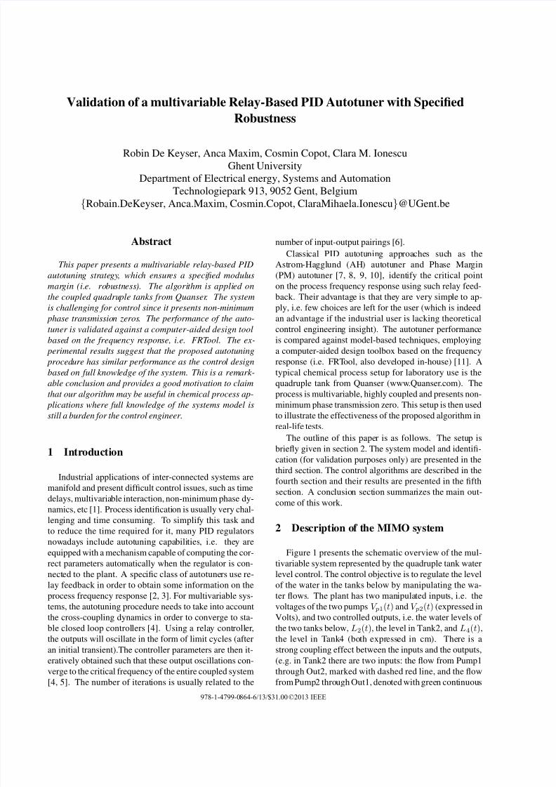
Figure 1 presents the schematic overview of the mul-tivariable system represented by the quadruple tank water

level control. The control objective is to regulate the level

of the water in the tanks below by manipulating the wa-

ter flows. The plant has two manipulated inputs, i.e. the

voltages of the two pumps V p1(t) and V p2(t) (expressed in

Volts), and two controlled outputs, i.e. the water levels of

the two tanks below, L2(t), the level in Tank2, and L4(t),

the level in Tank4 (both expressed in cm). There is a

strong coupling effect between the inputs and the outputs,

(e.g. in Tank2 there are two inputs: the flow from Pump1

through Out2, marked with dashed red line, and the flow

from Pump2 through Out1, denoted with green continuous

978-1-4799-0864-6/13/$31.00 ©2013 IEEE



line, that is the output flow from Tank1). Hence, the con-

trolled level in Tank2 is influenced by the two inputs, and

by adjusting the percentage of water flow from each input,

one can change the system for having minimum phase or

non-minimum phase dynamics.

Figure 1. Schematic diagram of the quadru-

ple tank process from Quanser

Based on the configuration depicted in Figure 1, in

Tank2 there is a greater flow coming from Pump2, via

Tank1, than the flow coming directly from Pump1. This

exotic situation originates from the fact that the outlet di-

ameter Out1 is bigger than the diameter Out2, while the

outgoing orifices from each tank Doi , i=1...4 have all the

same diameter. The same situation applies for Tank4. It

follows the conclusion that the dominant flow in the tanks

2 and 4 comes from the manner in which the physical cou-

pling is implemented via the choice of the setup.

3 Modelling and identification

In order to simplify matters, the modelling principle for

a single-input single output setup is given below, but it is

valid for the multivariable setup as well. The outflow from

Tank1 can be expressed as F o1 = Ao1vo1, with vo1 the

flow velocity.The cross-section area of the outflow orifice

in Tank1 can be expressed as Ao1 = 14πD2

o1, with Do1 the

diameter. Using Bernoullis equation, we have that:

F o1 = Ao1

√ 2

gL1 (1)

Using the mass balance equation in Tank1 it follows that

At1d

dtL1 = F i1 − F o1 (2)

Substituting for F i1 and F o1 we have that:

d

dtL1 =

K f V p − Ao1

√ 2√

gL1

At1. (3)

In steady-state, all time derivatives are zero and it re-

sults K f V p0 − Ao1

√ 2√

gL10 = 0. For any value of the

desired level in Tank1 (L10 = 10cm), the value of the

pump voltage in equilibrium can be calculated. Applying

linearization and Laplace transform, we have that:

L11

V p(s) =

K 1

τ 1s + 1, (4)

where K 1 = K f

√ 2√ gL10

Ao1g and τ 1 = At1

√ 2√ gL10

Ao1g Simi-larly, the outflow from Tank2 can be expressed as F o2 =Ao2vo2. The cross-section area of the outflow orifice

in Tank2 can be expressed as Ao2 = 14πD2

o2. Using

Bernoullis equation and the mass balance equation in

Tank2 it follows that:

At2

d

dtL2

= F i2 − F o2, (5)

Substituting for F i2 and F o2 assuming steady-state, it fol-

lows that:

L10 = A2

o2L20

A2

o1

. (6)

Applying linearization and Laplace transform, we have

that:L21

L11(s) =

K 2

τ 2s + 1, (7)

where K 2 = Ao1

√ L20

Ao2

√ L10

and τ 2 = At2

√ 2√ gL20

Ao2g .

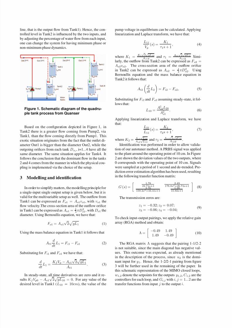
Identification was performed in order to allow valida-

tion of our autotuner method. A PRBS signal was applied

to the plant around the operating point of 10 cm. In Figure

2 are shown the deviation values of the two outputs, where

0 corresponds with the operating point of 10 cm. Signals

were sampled at a period of 1 second and de-trended. Pre-

diction error estimation algorithm has been used, resultingin the following transfer function matrix:

G (s) =

1.7822.71s+1

2.49178.8s2+26.74s+1

2.76159.2s2+33.41s+1

1.2815.92s+1

(8)

The transmission zeros are:

z1 = −0.32; z2 = 0.07;z3 = −0.06; z4 = −0.04;

(9)

To check input-output pairings, we apply the relative gain

array (RGA) method and obtain:

Λ = −0.49 1.49

1.49 −0.49

(10)

The RGA matrix Λ suggests that the pairing 1-1/2-2

is not suitable, since the main diagonal has negative val-

ues. This outcome was expected, as already mentioned

in the description of the process, since u2 is the domi-

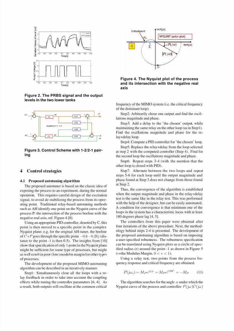
nant input for y1. Hence, the 1-2/2-1 pairing from figure

3 will be further used in the remaining of the paper. In

this schematic representation of the MIMO closed loops,

w1,2 denote the setpoints for the outputs y1,2, C 1,2 are the

controllers for each loop, and Gi,j with i, j = 1...2 are the

transfer functions from input j to the output i.



Figure 2. The PRBS signal and the outputlevels in the two lower tanks

Figure 3. Control Scheme with 1-2/2-1 pair-ing

4 Control strategies

4.1 Proposed autotuning algorithm

The proposed autotuner is based on the classic idea of

exposing the process to an experiment, during the normal

operation. This requires careful design of the excitation

signal, to avoid de-stabilizing the process from its oper-

ating point. Traditional relay-based autotuning methods

such as AH identify one point on the Nyquist curve of the

process P: the intersection of the process beeline with the

negative real axis, ref. Figure 4 [8].

Using an appropriate PID controller, denoted by C, this

point is then moved to a specific point in the complex

Nyquist plane; e.g. for the original AH-tuner, the beelineof C ∗P goes through the specific point −0.6−0.28 j (dis-

tance to the point -1 is then 0.5). The insights from [10]

show that specification of only 1 point in the Nyquist plane

might be sufficient for some type of processes, but might

as well result in poor (low) modulus margin for other types

of processes.

The development of the proposed MIMO autotuning

algorithm can be described in an iteratively manner.

Step1: Simultaneously close all the loops with a re-

lay feedback in order to take into account the coupling

effects while tuning the controller parameters [6, 4]. As

a result, both outputs will oscillate at the common critical

Figure 4. The Nyquist plot of the processand its intersection with the negative realaxis

frequency of the MIMO system (i.e. the critical frequency

of the dominant loop).

Step2: Arbitrarily chose one output and find the oscil-

lations magnitude and phase.

Step3: Add a delay to the ’the chosen’ output, while

maintaining the same relay on the other loop (as in Step1).

Find the oscillations magnitude and phase for the re-

lay+delay loop.

Step4: Compute a PID controller for ’the chosen’ loop.

Step5: Replace the relay+delay from the loop selected

at step 2 with the computed controller (Step 4). Find for

the second loop the oscillations magnitude and phase.

Step6: Repeat steps 3-4 (with the mention that the

other loop is closed with PID).

Step7: Alternate between the two loops and repeat

steps 5-6 for each loop until the output magnitude and

phase found at Step 3 does not change from those found

at Step 2.

Thus, the convergence of the algorithm is established

when the output magnitude and phase in the relay+delay

test is the same like in the relay test. This was performed

with the help of the designer, but can be easily automated.

A condition for convergence is that minimum one of the

loops in the system has a characteristic locus with at least

180 degrees phase lag [4, 5].

The controllers from this paper were obtained after

four iterations of the above procedure. Next, the method-

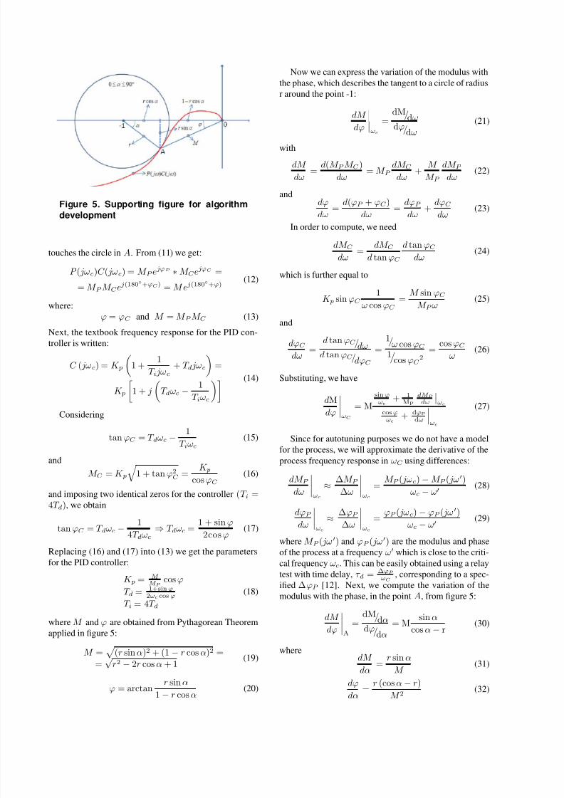
ology behind steps 2-4 is presented. The development of the proposed autotuning algorithm is based on imposing

a user-specified robustness. The robustness specification

can be translated using Nyquist plots as a circle of spec-

ified radius (r) around the point -1 as drawn in Figure 5

(r=the Modulus Margin, 0 < r < 1).

Using a relay test, two points from the process fre-

quency response and critical frequency are obtained.

P ( jωc) = M P ejϕP = M P e

j180◦ = −M P (11)

The algorithm searches for the angle α under which the

Nyquist curve of the process and controller P ( jω)C ( jω)



Figure 5. Supporting figure for algorithmdevelopment

touches the circle in A. From (11) we get:

P ( jωc)C ( jωc) = M P ejϕP

∗M C e

jϕC =

= M P M C ej(180◦+ϕC) = M ej(180

◦+ϕ) (12)

where:

ϕ = ϕC and M = M P M C (13)

Next, the textbook frequency response for the PID con-

troller is written:

C ( jωc) = K p

1 +

1

T i jωc+ T d jωc

=

K p

1 + j

T dωc − 1

T iωc

(14)

Considering

tan ϕC = T dωc − 1

T iωc(15)

and

M C = K p

1 + tan ϕ2

C = K p

cos ϕC (16)

and imposing two identical zeros for the controller (T i =4T d), we obtain

tan ϕC = T dωc − 1

4T dωc⇒ T dωc =

1 + sin ϕ

2cos ϕ (17)

Replacing (16) and (17) into (13) we get the parameters

for the PID controller:

K p = M M P

cos ϕ

T d = 1+sinϕ2ωc cos ϕ

T i = 4T d

(18)

where M and ϕ are obtained from Pythagorean Theorem

applied in figure 5:

M =

(r sin α)2 + (1 − r cos α)2 =

=√

r2 − 2r cos α + 1 (19)

ϕ = arctan r sin α

1 − r cos α

(20)

Now we can express the variation of the modulus with

the phase, which describes the tangent to a circle of radius

r around the point -1:

dM

dϕ

ωc

=dM/dωdϕ/dω

(21)

with

dM

dω =

d(M P M C )

dω = M P

dM C

dω +

M

M P

dM P

dω (22)

anddϕ

dω =

d(ϕP + ϕC )

dω =

dϕP

dω +

dϕC

dω (23)

In order to compute, we need

dM C

dω =

dM C

d tan ϕC

d tan ϕC

dω (24)

which is further equal to

K p sin ϕC 1

ω cos ϕC =

M sin ϕC

M P ω (25)

and

dϕC

dω =

d tan ϕC /dωd tan ϕC /dϕC

=1/ω cos ϕC

1

cos ϕC 2

= cos ϕC

ω (26)

Substituting, we have

dM

dϕ

ωC

= M

sinϕωc

+ 1MP

dM P dω

ωc

cosϕ

ωc +

dϕP

dωωc

(27)

Since for autotuning purposes we do not have a model

for the process, we will approximate the derivative of the

process frequency response in ωC using differences:

dM P

dω

ωc

≈ ∆M P

∆ω

ωc

= M P ( jωc)− M P ( jω )

ωc − ω (28)

dϕP

dω

ωc

≈ ∆ϕP

∆ω

ωc

= ϕP ( jωc) − ϕP ( jω )

ωc − ω (29)

where M P ( jω ) and ϕP ( jω ) are the modulus and phase

of the process at a frequency ω which is close to the criti-

cal frequency ωc. This can be easily obtained using a relay

test with time delay, τ d = ∆ϕP

ωC, corresponding to a spec-

ified ∆ϕP [12]. Next, we compute the variation of the

modulus with the phase, in the point A, from figure 5:

dM

dϕ

A

=dM/dαdϕ/dα

= M sin α

cos α− r (30)

wheredM

dα =

r sin α

M (31)

dϕ

dα

= r (cos α− r)

M 2

(32)



Then, by finding iteratively the angle ∝∗ for which the

error

dM dϕ

ωC

− dM dϕ

A

is minimum, we obtain the opti-

mal parameters of the controller for a specified modulus

margin r.

The procedure presented above, can be summarized as:

1) Find ωc and M P (ωc) via relay test [ϕc = −180◦]2) Find ω

c, M P (ωc) and ϕP (ω

c) via a relay+delay test

3) Calculate ∆M P ∆ω

and ∆ϕP ∆ω

4) For α = 0...90◦, calculate M (α), ϕ(α) and

δ (α) =

dM dϕ

ωC

− dM dϕ

A

5) Calculate M (α∗) and ϕ(α∗) with

α∗ = arg minαδ (α)6) Calculate {K p, T i, T d}.

This method of autotuning has been successfully vali-

dated on numerous examples for single input-single out-

put systems [12, 13].

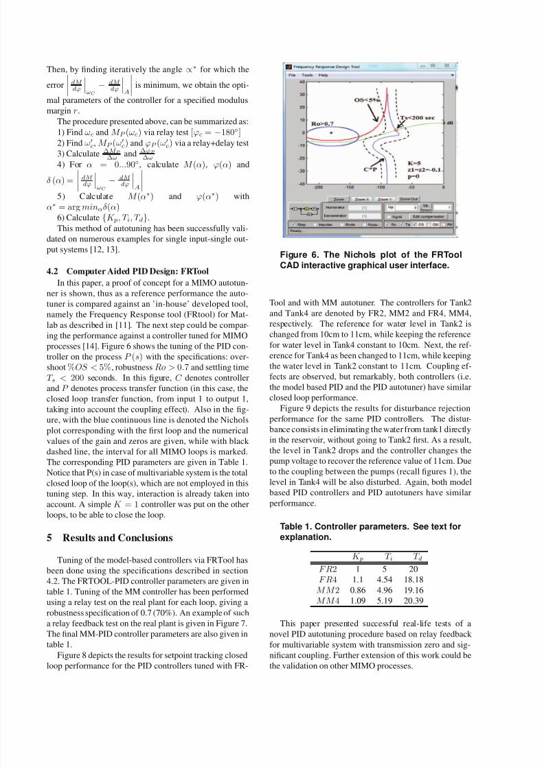
4.2 Computer Aided PID Design: FRToolIn this paper, a proof of concept for a MIMO autotun-

ner is shown, thus as a reference performance the auto-

tuner is compared against an ’in-house’ developed tool,

namely the Frequency Response tool (FRtool) for Mat-

lab as described in [11]. The next step could be compar-

ing the performance against a controller tuned for MIMO

processes [14]. Figure 6 shows the tuning of the PID con-

troller on the process P (s) with the specifications: over-

shoot %OS < 5%, robustness Ro > 0.7 and settling time

T s < 200 seconds. In this figure, C denotes controller

and P denotes process transfer function (in this case, the

closed loop transfer function, from input 1 to output 1,

taking into account the coupling effect). Also in the fig-

ure, with the blue continuous line is denoted the Nichols

plot corresponding with the first loop and the numerical

values of the gain and zeros are given, while with black

dashed line, the interval for all MIMO loops is marked.

The corresponding PID parameters are given in Table 1.

Notice that P(s) in case of multivariable system is the total

closed loop of the loop(s), which are not employed in this

tuning step. In this way, interaction is already taken into

account. A simple K = 1 controller was put on the other

loops, to be able to close the loop.

5 Results and Conclusions

Tuning of the model-based controllers via FRTool has

been done using the specifications described in section

4.2. The FRTOOL-PID controller parameters are given in

table 1. Tuning of the MM controller has been performed

using a relay test on the real plant for each loop, giving a

robustness specification of 0.7 (70%). An example of such

a relay feedback test on the real plant is given in Figure 7.

The final MM-PID controller parameters are also given in

table 1.

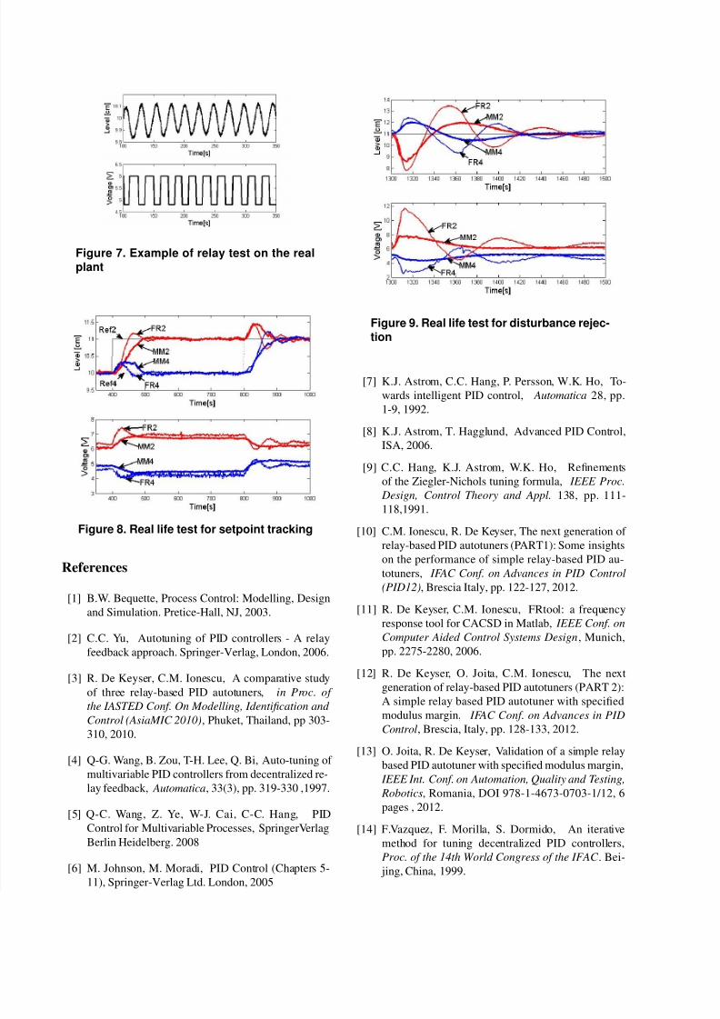
Figure 8 depicts the results for setpoint tracking closed

loop performance for the PID controllers tuned with FR-

Figure 6. The Nichols plot of the FRTool

CAD interactive graphical user interface.

Tool and with MM autotuner. The controllers for Tank2

and Tank4 are denoted by FR2, MM2 and FR4, MM4,

respectively. The reference for water level in Tank2 is

changed from 10cm to 11cm, while keeping the reference

for water level in Tank4 constant to 10cm. Next, the ref-

erence for Tank4 as been changed to 11cm, while keeping

the water level in Tank2 constant to 11cm. Coupling ef-

fects are observed, but remarkably, both controllers (i.e.

the model based PID and the PID autotuner) have similar

closed loop performance.

Figure 9 depicts the results for disturbance rejection

performance for the same PID controllers. The distur-

bance consists in eliminating the water from tank1 directly

in the reservoir, without going to Tank2 first. As a result,

the level in Tank2 drops and the controller changes the

pump voltage to recover the reference value of 11cm. Due

to the coupling between the pumps (recall figures 1), the

level in Tank4 will be also disturbed. Again, both model

based PID controllers and PID autotuners have similar

performance.

Table 1. Controller parameters. See text for

explanation.

K p T i T d

F R2 1 5 20

F R4 1.1 4.54 18.18

M M 2 0.86 4.96 19.16

M M 4 1.09 5.19 20.39

This paper presented successful real-life tests of a

novel PID autotuning procedure based on relay feedback

for multivariable system with transmission zero and sig-

nificant coupling. Further extension of this work could be

the validation on other MIMO processes.



Figure 7. Example of relay test on the realplant

Figure 8. Real life test for setpoint tracking

References

[1] B.W. Bequette, Process Control: Modelling, Design

and Simulation. Pretice-Hall, NJ, 2003.

[2] C.C. Yu, Autotuning of PID controllers - A relay

feedback approach. Springer-Verlag, London, 2006.

[3] R. De Keyser, C.M. Ionescu, A comparative study

of three relay-based PID autotuners, in Proc. of

the IASTED Conf. On Modelling, Identification and

Control (AsiaMIC 2010), Phuket, Thailand, pp 303-

310, 2010.

[4] Q-G. Wang, B. Zou, T-H. Lee, Q. Bi, Auto-tuning of

multivariable PID controllers from decentralized re-

lay feedback, Automatica, 33(3), pp. 319-330 ,1997.

[5] Q-C. Wang, Z. Ye, W-J. Cai, C-C. Hang, PID

Control for Multivariable Processes, SpringerVerlag

Berlin Heidelberg. 2008

[6] M. Johnson, M. Moradi, PID Control (Chapters 5-

11), Springer-Verlag Ltd. London, 2005

Figure 9. Real life test for disturbance rejec-tion

[7] K.J. Astrom, C.C. Hang, P. Persson, W.K. Ho, To-

wards intelligent PID control, Automatica 28, pp.

1-9, 1992.

[8] K.J. Astrom, T. Hagglund, Advanced PID Control,

ISA, 2006.

[9] C.C. Hang, K.J. Astrom, W.K. Ho, Refinements

of the Ziegler-Nichols tuning formula, IEEE Proc.

Design, Control Theory and Appl. 138, pp. 111-

118,1991.

[10] C.M. Ionescu, R. De Keyser, The next generation of relay-based PID autotuners (PART1): Some insights

on the performance of simple relay-based PID au-

totuners, IFAC Conf. on Advances in PID Control

(PID12), Brescia Italy, pp. 122-127, 2012.

[11] R. De Keyser, C.M. Ionescu, FRtool: a frequency

response tool for CACSD in Matlab, IEEE Conf. on

Computer Aided Control Systems Design, Munich,

pp. 2275-2280, 2006.

[12] R. De Keyser, O. Joita, C.M. Ionescu, The next

generation of relay-based PID autotuners (PART 2):

A simple relay based PID autotuner with specified

modulus margin, IFAC Conf. on Advances in PIDControl, Brescia, Italy, pp. 128-133, 2012.

[13] O. Joita, R. De Keyser, Validation of a simple relay

based PID autotuner with specified modulus margin,

IEEE Int. Conf. on Automation, Quality and Testing,

Robotics, Romania, DOI 978-1-4673-0703-1/12, 6

pages , 2012.

[14] F.Vazquez, F. Morilla, S. Dormido, An iterative

method for tuning decentralized PID controllers,

Proc. of the 14th World Congress of the IFAC . Bei-

jing, China, 1999.

validation of a multivariable relay-based pid autotuner with specified

Documents