validation of a fully automated 3d hippocampal...

1

Validation of a Fully Automated 3D Hippocampal Segmentation Method Using Subjects

with Alzheimer’s Disease, Mild Cognitive Impairment, and Elderly Controls

Jonathan H. Morra MS1, Zhuowen Tu PhD1, Liana G. Apostolova MD1,2, Amity E. Green1,2,Christina Avedissian1, Sarah K. Madsen1, Neelroop Parikshak1, Xue Hua MS1, Arthur W. Toga PhD1,

Clifford R. Jack Jr MD3, Michael W. Weiner MD4,5, Paul M. Thompson PhD1

and the Alzheimer’s Disease Neuroimaging Initiative*

1Laboratory of Neuro Imaging, Dept. of Neurology, UCLA School of Medicine, Los Angeles, CA2Dept. of Neurology, UCLA School of Medicine, Los Angeles, CA

3Mayo Clinic College of Medicine, Rochester, MN4Dept. Radiology, and 5Dept. Medicine and Psychiatry, UC San Francisco, San Francisco, CA

Submitted to NeuroImage: December 3, 2007Revised Version submitted: February 9, 2008

2nd Revision submitted: May 26, 2008

Please address correspondence to:Dr. Paul Thompson, Professor of Neurology

Laboratory of Neuro Imaging, Dept. of Neurology,UCLA School of Medicine

Neuroscience Research Building 225E635 Charles Young Drive, Los Angeles, CA 90095-1769, USA

Phone: (310) 206-2101 Fax: (310) 206-5518 E-mail: [email protected]

*Acknowledgments and Author Contributions: Data used in preparing this article were obtained from the Alzheimer's DiseaseNeuroimaging Initiative database (www.loni.ucla.edu/ADNI). Many ADNI investigators therefore contributed to the design andimplementation of ADNI or provided data but did not participate in the analysis or writing of this report. A complete listing ofADNI investigators is available at www.loni.ucla.edu/ADNI/Collaboration/ADNI_Citation.shtml. This work was primarilyfunded by the ADNI (Principal Investigator: Michael Weiner; NIH grant number U01 AG024904). ADNI is funded by theNational Institute of Aging, the National Institute of Biomedical Imaging and Bioengineering (NIBIB), and the Foundation forthe National Institutes of Health, through generous contributions from the following companies and organizations: Pfizer Inc.,Wyeth Research, Bristol-Myers Squibb, Eli Lilly and Company, GlaxoSmithKline, Merck & Co. Inc., AstraZeneca AB, NovartisPharmaceuticals Corporation, the Alzheimer’s Association, Eisai Global Clinical Development, Elan Corporation plc, ForestLaboratories, and the Institute for the Study of Aging (ISOA), with participation from the U.S. Food and Drug Administration.The grantee organization is the Northern California Institute for Research and Education, and the study is coordinated by theAlzheimer’s Disease Cooperative Study at the University of California, San Diego. Algorithm development for this study wasalso funded by the NIA, NIBIB, the National Library of Medicine, and the National Center for Research Resources (AG016570,EB01651, LM05639, RR019771 to PT). Author contributions were as follows: JM, ZT, LA, AG, CA, SM, NP, XH, AT, and PTperformed the image analyses; CJ, NS, and MW contributed substantially to the image acquisition, study design, quality control,calibration and pre-processing, databasing and image analysis. We thank the members of the ADNI Imaging Core for theircontributions to the image pre-processing and the ADNI project.

2

Abstract: (250; max: 250 words)

We introduce a new method for brain MRI segmentation, called the auto context model (ACM),

to segment the hippocampus automatically in 3D T1-weighted structural brain MRI scans of

subjects from the Alzheimer’s Disease Neuroimaging Initiative (ADNI). In a training phase,

our algorithm used 21 hand-labeled segmentations to learn a classification rule for

hippocampal versus non-hippocampal regions using a modified AdaBoost method, based

on ~18,000 features (image intensity, position, image curvatures, image gradients, tissue

classification maps of gray/white matter and CSF, and mean, standard deviation, and Haar

filters of size 1x1x1 to 7x7x7). We linearly registered all brains to a standard template to

devise a basic shape prior to capture the global shape of the hippocampus, defined as the

pointwise summation of all the training masks. We also included curvature, gradient,

mean, standard deviation, and Haar filters of the shape prior and the tissue classified

images as features. During each iteration of ACM - our extension of AdaBoost - the

Bayesian posterior distribution of the labeling was fed back in as an input, along with its

neighborhood features, as new features for AdaBoost to use. In validation studies, we

compared our results with hand-labeled segmentations by two experts. Using a leave-one-

out approach and standard overlap and distance error metrics, our automated

segmentations agreed well with human raters; any differences were comparable to

differences between trained human raters. Our error metrics compare favorably with

those previously reported for other automated hippocampal segmentations, suggesting the

utility of the approach for large-scale studies.

Introduction:

Alzheimer’s disease (AD) is the most common type of dementia, and affects over 5 million

people in the United States alone (Jorm et al., 1987). The disease is associated with the

pathological accumulation of amyloid plaques and neurofibrillary tangles in the brain, and first

affects memory systems, progressing to involve language, affect, executive function, and all

aspects of behavior. A major therapeutic goal is to assess whether treatments delay or resist

3

disease progression in the brain before widespread cortical and subcortical damage occurs. For

this, sensitive neuroimaging measures have been sought to quantify structural changes in the

brain in early AD which are automated enough to permit large-scale studies of disease and the

factors that affect it.

To track the disease process, several MRI- or PET-based imaging measures have been proposed.

Many studies have sought optimal volumetric measures (e.g., of the hippocampus or entorhinal

cortex) to differentiate normal aging from AD, and from mild cognitive impairment (MCI), a

transitional state that carries a 4-6 fold increased risk of imminent decline to AD relative to the

normal population (Petersen, 2000; Petersen et al., 2001; Petersen et al., 1999). A common

biological marker of disease progression is morphological change in the hippocampus, assessed

using volumetric measures (Jack et al., 1999; Kantarci and Jack, 2003) or by mapping the spatial

distribution of atrophy in 3D (Apostolova et al., 2006a; Apostolova et al., 2006b; Csernansky et

al., 1998; Frisoni et al., 2006; Thompson et al., 2004).

Using MRI at millimeter resolution, subtle hippocampal shape changes may be resolved.

However, isolating the hippocampus in a large number of MRI scans is time-consuming, and

most studies still rely on manual outlining guided by expert knowledge of the location and shape

of each region of interest (ROI) (Apostolova et al., 2006a; Du et al., 2001). To accelerate

epidemiological studies and clinical trials, this process should be automated. Some automated

systems have been proposed for hippocampal segmentation (Barnes et al., 2004; Crum et al.,

2001; Fischl et al., 2002; Hogan et al., 2000; Powell et al., 2008; Wang et al., 2007; Yushkevich

et al., 2006), but none is yet widely used.

Pattern recognition techniques (Duda et al., 2001) offer a range of promising algorithms for

automated subcortical segmentation. Most pattern recognition (or machine learning) algorithms

attempt to assign a probability to a specific outcome. In image segmentation, image cues are

pooled to determine with a specific probability whether each image voxel is part of an ROI (e.g.,

the hippocampus) or not. In pattern recognition, cues are usually referred to as features, and

different pattern recognition algorithms combine these features in different ways. When using

pattern recognition approaches, it is standard practice to divide a dataset into two non-

4

overlapping classes, for training and testing. The training set is used to learn the patterns (e.g.,

estimate a function or decision rule for classifying voxels), and the testing set is used to validate

how well new datasets can be classified, based on the patterns that were learned.

Since medical images are complex, many possible features may be created to represent each

voxel. Given the large number of voxels in an MRI scan, computing and storing this amount of

data may become unmanageable. For example, features may consist of image intensity, x, y, and

z positions, image curvature, image gradients, or the output of any other general image filter. To

overcome this problem, here we use a variant of a machine learning algorithm called AdaBoost

(Freund and Schapire, 1997). AdaBoost is a weighted voting algorithm, which combines “weak

learners” into a “strong learner.” A weak learner is any pattern recognition algorithm that

guesses correctly greater than half of the time. At each iteration, AdaBoost selects a weak

learner that minimizes the error for all voxels based on the classification of previously selected

weak learners. Therefore, an incorrectly classified example at one iteration will receive more

weight on subsequent iterations.

To segment the hippocampus in an MRI scan, here we use AdaBoost inside a new pattern

recognition algorithm we call the auto context model (ACM). ACM is not specific to AdaBoost

and may be used with any classification technique, but here we use it with AdaBoost, which has

previously been found to be effective for subcortical segmentation in smaller samples of subjects

(Morra et al., 2007; Quddus et al., 2005; Tu et al., 2007).

This paper presents a validation study of ACM using data from an Alzheimer’s disease

study. We show that this approach accurately captures the hippocampus and may

therefore be useful in large scale studies of AD where manual tracing would be prohibitive.

Methods:

Subjects

5

The Alzheimer’s Disease Neuroimaging Initiative (ADNI) (Mueller et al., 2005a; Mueller et al.,

2005b) is a large multi-site longitudinal MRI and FDG-PET (fluorodeoxyglucose positron

emission tomography) study of 800 adults, ages 55 to 90, including 200 elderly controls, 400

subjects with mild cognitive impairment, and 200 patients with AD. The ADNI was launched in

2003 by the National Institute on Aging (NIA), the National Institute of Biomedical Imaging and

Bioengineering (NIBIB), the Food and Drug Administration (FDA), private pharmaceutical

companies and non-profit organizations, as a $60 million, 5-year public-private partnership. The

primary goal of ADNI has been to test whether serial MRI, PET, other biological markers, and

clinical and neuropsychological assessment can be combined to measure the progression of MCI

and early AD. Determination of sensitive and specific markers of very early AD progression is

intended to aid researchers and clinicians to develop new treatments and monitor their

effectiveness, as well as lessen the time and cost of clinical trials. The Principal Investigator of

this initiative is Michael W. Weiner, M.D., VA Medical Center and University of California –

San Francisco.

All subjects underwent thorough clinical/cognitive assessment at the time of scan acquisition.

As part of each subject’s cognitive evaluation, the Mini-Mental State Examination (MMSE) was

administered to provide a global measure of cognitive status based on evaluation of five

cognitive domains (Cockrell and Folstein, 1988; Folstein et al., 1975); scores of 24 or less (out of

a maximum of 30) are generally consistent with dementia. Two versions of the Clinical

Dementia Rating (CDR) were also used as a measure of dementia severity (Hughes et al., 1982;

Morris, 1993). The global CDR represents the overall level of dementia, and a global CDR of 0,

0.5, 1, 2 and 3, respectively, indicate no dementia, very mild, mild, moderate, or severe

dementia. The “sum-of-boxes” CDR score is the sum of 6 scores assessing different areas of

cognitive function: memory, orientation, judgment and problem solving, community affairs,

home and hobbies, and personal care. The sum of these scores ranges from 0 (no dementia) to

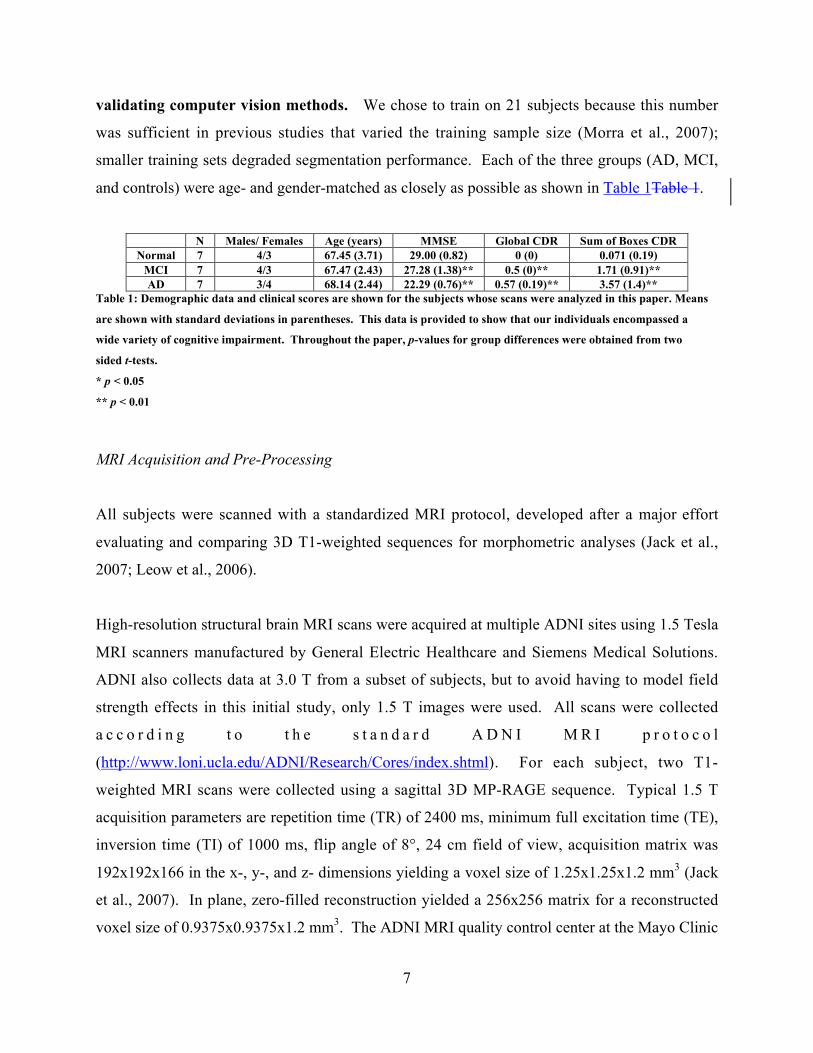
18 (very severe dementia). Table 1 shows the clinical scores and demographic measures for our

sample. The elderly normal subjects in our sample had MMSE scores between 26 and 30, a

global CDR of 0, a sum-of-boxes CDR between 0 and 0.5, and no other signs of MCI or other

forms of dementia. The MCI subjects had MMSE scores ranging from 24 to 30, a global CDR of

0.5, a sum-of-boxes CDR score between 0.5 and 5, and mild memory complaints. Memory

6

impairment was assessed via education-adjusted scores on the Wechsler Memory Scale - Logical

Memory II (Wechsler, 1987). All AD patients met NINCDS/ADRDA criteria for probable AD

(McKhann et al., 1984) with an MMSE score between 20 and 26, a global CDR between 0.5 and

1, and a sum-of-boxes CDR between 1.0 and 9.0. As such, these subjects would be considered

as having mild, but not severe, AD. Detailed exclusion criteria, e.g., regarding concurrent use of

psychoactive medications, may be found in the ADNI protocol (page 29, http://www.adni-

info.org/images/stories/Documentation/adni_protocol_03.02.2005_ss.pdf). Briefly, subjects

were excluded if they had any serious neurological disease other than incipient AD, any history

of brain lesions or head trauma, or psychoactive medication use (including antidepressants,

neuroleptics, chronic anxiolytics or sedative hypnotics, etc.).

The study was conducted according to Good Clinical Practice, the Declaration of Helsinki and

U.S. 21 CFR Part 50-Protection of Human Subjects, and Part 56-Institutional Review Boards.

Written informed consent for the study was obtained from all participants before protocol-

specific procedures, including cognitive testing, were performed.

Training and Testing Set Descriptions

As noted earlier, when using a pattern recognition approach to identify structures in images, two

non-overlapping sets of images must be defined, for training and testing (Morra et al., 2007;

Powell et al., 2008). The training set consists of a small sample of brain images, representative

of the entire dataset, which are manually traced by experts. The testing set is a group of brain

images that are to be segmented by the algorithm, but have not been used for training the

algorithm. Our training set consisted of 21 brain images, from 7 healthy elderly individuals, 7

individuals with MCI, and 7 individuals with AD. Since we only have manual tracings of

these brains, we construct our testing set using a leave-one-out approach. For testing, we

train 21 models, each one ignoring one subject (i.e., not using that subject for training), and

we then test each model on the subject that it ignored. This gives a testing set of the same

21 brains, each with a ground truth segmentation for comparison purposes; even so, it

ensures the independence of the training and testing sets, a common requirement in

7

validating computer vision methods. We chose to train on 21 subjects because this number

was sufficient in previous studies that varied the training sample size (Morra et al., 2007);

smaller training sets degraded segmentation performance. Each of the three groups (AD, MCI,

and controls) were age- and gender-matched as closely as possible as shown in Table 1Table 1.

N Males/ Females Age (years) MMSE Global CDR Sum of Boxes CDRNormal 7 4/3 67.45 (3.71) 29.00 (0.82) 0 (0) 0.071 (0.19)

MCI 7 4/3 67.47 (2.43) 27.28 (1.38)** 0.5 (0)** 1.71 (0.91)**AD 7 3/4 68.14 (2.44) 22.29 (0.76)** 0.57 (0.19)** 3.57 (1.4)**

Table 1: Demographic data and clinical scores are shown for the subjects whose scans were analyzed in this paper. Means

are shown with standard deviations in parentheses. This data is provided to show that our individuals encompassed a

wide variety of cognitive impairment. Throughout the paper, p-values for group differences were obtained from two

sided t-tests.

* p < 0.05

** p < 0.01

MRI Acquisition and Pre-Processing

All subjects were scanned with a standardized MRI protocol, developed after a major effort

evaluating and comparing 3D T1-weighted sequences for morphometric analyses (Jack et al.,

2007; Leow et al., 2006).

High-resolution structural brain MRI scans were acquired at multiple ADNI sites using 1.5 Tesla

MRI scanners manufactured by General Electric Healthcare and Siemens Medical Solutions.

ADNI also collects data at 3.0 T from a subset of subjects, but to avoid having to model field

strength effects in this initial study, only 1.5 T images were used. All scans were collected

a c c o r d i n g t o t h e s t a n d a r d A D N I M R I p r o t o c o l

(http://www.loni.ucla.edu/ADNI/Research/Cores/index.shtml). For each subject, two T1-

weighted MRI scans were collected using a sagittal 3D MP-RAGE sequence. Typical 1.5 T

acquisition parameters are repetition time (TR) of 2400 ms, minimum full excitation time (TE),

inversion time (TI) of 1000 ms, flip angle of 8°, 24 cm field of view, acquisition matrix was

192x192x166 in the x-, y-, and z- dimensions yielding a voxel size of 1.25x1.25x1.2 mm3 (Jack

et al., 2007). In plane, zero-filled reconstruction yielded a 256x256 matrix for a reconstructed

voxel size of 0.9375x0.9375x1.2 mm3. The ADNI MRI quality control center at the Mayo Clinic

8

(in Rochester, MN, USA) selected the MP-RAGE image with higher quality based on

standardized criteria (Jack et al., 2007). Additional phantom-based geometric corrections were

applied to ensure spatial calibration was kept within a specific tolerance level for each scanner

involved in the ADNI study (Gunter et al., 2006).

Additional image corrections were also applied, using a processing pipeline at the Mayo Clinic,

consisting of: (1) a procedure termed GradWarp for correction of geometric distortion due to

gradient non-linearity (Jovicich et al., 2006), (2) a “B1-correction”, to adjust for image intensity

non-uniformity using B1 calibration scans (Jack et al., 2007), (3) “N3” bias field correction, for

reducing intensity inhomogeneity (Sled et al., 1998), and (4) geometrical scaling, according to a

phantom scan acquired for each subject (Jack et al., 2007), to adjust for scanner- and session-

specific calibration errors. In addition to the original uncorrected image files, images with all of

these corrections already applied (GradWarp, B1, phantom scaling, and N3) are available to the

general scientific community, as described at http://www.loni.ucla.edu/ADNI. Ongoing studies

are examining the influence of N3 parameter settings on measures obtained from ADNI scans

(Boyes et al., 2007).

Image Pre-processing

To adjust for global differences in brain positioning and scale across individuals, all scans were

linearly registered to the stereotactic space defined by the International Consortium for Brain

Mapping (ICBM-53) (Mazziotta et al., 2001) with a 9-parameter (9P) transformation (3

translations, 3 rotations, 3 scales) using the Minctracc algorithm (Collins et al., 1994). Globally

aligned images were resampled in an isotropic space of 220 voxels along each axis (x, y, and z)

with a final voxel size of 1 mm3.

Feature Selection

All discriminative pattern recognition techniques involve taking some set of examples with a

label and learning a pattern based on those examples. Usually the examples are themselves each

a vector of problem-specific information, referred to as features. Each feature must be calculable

9

for each example (for implementation purposes, hopefully quickly), and the features should

provide some insight into the classification task. For medical image segmentation, these features

are derived at each voxel in all brains, so at each voxel, there exists a vector for which each entry

is a specific feature evaluated at that voxel.

In our case, we chose features based on image intensity, tissue classification maps of gray matter,

white matter, and CSF (binary maps obtained by an unsupervised classifier, PVC (partial volume

classifier; (Shattuck et al., 2001))) and neighborhood-based features derived from the tissue

classified maps, x, y, and z positions (along with combinations of positions such as x+y or x*z),

curvature filters, gradient filters, mean filters, standard deviation filters, and Haar filters (Viola

and Jones, 2004) of sizes varying from 1x1x1 to x , y, z positions were determined using

stereotaxic coordinates after spatial normalization to the standard space. In addition to these

features, we exploited the fact that all the brains had been registered to devise a basic shape prior

to capture the global shape of the hippocampus. Our shape prior was defined as the pointwise

summation of all the training masks. Differential positional effects in the x, y, and z positions are

therefore captured by using a shape prior, and also by including products of x, y, and z voxel

indices as features.

Since brain MRIs consist of many voxels, the product of the number of features and the number

of voxels can be exceedingly large. However, because all of our brains are registered to the

same template, the hippocampi will always appear in approximately the same localized region.

We can exploit this fact to reduce our search space by constructing a bounding box, and only

classifying examples (feature vectors at each voxel) for voxels that fall in this bounding box. To

define the box we scan over all the training examples and find the minimum and maximum x, y, z

positions of the hippocampus. Next, we add the size of the largest neighborhood feature (in this

case, 7 voxels) and some additional voxels to cope with as yet unseen testing brains (in this case,

10 voxels). Then training commences on only voxels inside of this box. Also, when testing a

new brain, only voxels inside this box are classified, all others are assumed negative. All

features are computed at each voxel, rather than averaging them over the bounding box. When

classifying each voxel, features such as image intensity, image gradient, and tissue classification

are computed voxel-wise. The number of features is approximately 18,000 per voxel, and the

10

same set of candidate features are available to the classifier at every voxel, so the number of

features does not depend on the size of the bounding box.

AdaBoost Description

AdaBoost is a machine learning method that uses a training set of data to develop rules for

classifying future data; it combines individual rules that do not work especially well into a pool

of rules that can be used to more accurately classify new data. The overall classifier can greatly

outperform the component classifiers. The component classifiers are often called “weak

learners”, as they may perform only slightly better than random; for example, a classifier of

hippocampal voxels based on the binary feature “voxel is gray matter” could classify the

hippocampus only slightly better than chance (i.e., 50% correct), as there are many non-

hippocampal gray matter voxels. AdaBoost iteratively selects weak learners, h(x), from a

candidate pool and combines them into a strong learner, H(x) (Freund and Schapire, 1997). In

what follows, an example is defined as the feature vector at a voxel in the training dataset, with

its associated classification; a weak learner classifies example voxels as belonging to the

hippocampus or not belonging to the hippocampus. When classifying an example, a weak

learner gives a binary output value of +1 for example voxels that it regards as positive (i.e., in the

hippocampus) and -1 for example voxels it regards as negative (i.e., outside the hippocampus).

11

Figure 1: An overview of the AdaBoost algorithm. 1 is an indicator function, returning 1 if the statement is true and 0

otherwise.

Figure 1 gives an overview of the AdaBoost algorithm. In our implementation, labeling the

hippocampus is formulated as a two-class classification problem, in which the training data

consists of input vectors of features, Nxx ...1 , also called examples, and associated labels, yi. The

components of the features are the outputs of the Haar filters, intensity measures, positions, and

other feature detectors detailed earlier. The training phase of AdaBoost attempts to find the best

combination of classifiers. Each data point, or example, is initially given a weight, D1(i). The

weighting parameter for each data point is initially set to 1/N for all data points.

At this point, the construction of the set of weak learners hj (of size J) needs to be defined. We

define a weak learner to be any feature, a threshold, and a boolean function representing whether

or not observations above that threshold are positive (belong to the ROI) or negative (do not

12

belong to the ROI). Therefore, our weak learner selects the feature that best separates the data

into positive and negative examples given Dt. In order to do this, two histograms are constructed

for each feature based on Dt, one that is only the positive examples, and another that is only the

negative examples, these are then normalized and converted into cumulative distribution

functions (CDFs). Finally, the threshold that minimizes the error based on these CDFs is chosen,

and the lowest error over all features determines which weak learner is selected.

More formally, as detailed in Figure 1, at each stage t of the algorithm (t = 1 to T), AdaBoost

trains a new weak learner in which the weighting coefficients, Dt(i), on the example data points

are adjusted to give greater weight to the previously misclassified data points. In Figure 1Figure

1, ε j is the total error of the jth weak learner, determined by counting up all the examples

misclassified, 1(yi ≠ hj(xi)), weighted by their current weights at time t, Dt(i). As such, they are

weighted measures of the error rates of the weak learners. The best weak learner for stage t is

the one with the lowest error, εt. This learner is based on a feature that is most “independent” of

the previous learners. The best weak learner at each step is chosen from the full set of weak

learners, not just from the new ones computed in successive steps by AdaBoost. The coefficient

)/)1log(()2/1( ttt εεα −= is defined to be a weighting coefficient for the t-th weak learner,

which favors learners with very low error. The key to AdaBoost is that the influence of each

example in the training set is re-weighted using the following rule: tititt ZxhyD /))(exp( α− , with

Zt a normalizer defined in Figure 1Figure 1, chosen so that the Dt+1(i) will be a probability

distribution, i.e., sum to 1 over all examples xi. This re-weighting emphasizes examples that

were wrongly labeled at the prior iteration. Successive classifiers are therefore forced to

prioritize examples that were incorrectly classified, and these data points receive increasing

priority, Dt(i). The formula for αt chosen such that it is the unique αt that minimizes Zt

analytically, by satisfying 0/)( =ttt ddZ αα ; picked in this way αt is guaranteed to minimize Zt.

The final vote H(x) is based on a thresholded weighted sum of all weak learners (Figure 1).

Because of the large number of examples to be classified, instead of using AdaBoost just once, a

cascade was created, where at each node in the cascade examples that are clearly negative are

discarded (a probability below 0.1). This allows the classifier to use different features for

13

examples that are difficult to classify. The value of 0.1 was chosen because it was empirically

shown to give good results in our other studies (Morra et al., 2007).

Probabilistic Interpretation

Friedman et al. (Friedman et al., 2000) noted that the update rule for weights (the “boosting”

steps) in AdaBoost can be given a probabilistic interpretation, i.e. it can be derived by assuming

that the goal is to sequentially minimize an exponential error function. Given a linear

combination of weak learners ∑ ==

T

t tt xhxf1

)()( rrα , then the exponential error of a mislabeling

may be defined as ∑ =−=

N

n nyn xfyE1

))(exp( r , where yi are the training set target values. If we

wish to minimize E by optimizing the weak learner ht( ), then it can be shown that the best re-

weighting of the examples is given by the update rule for Dt+1(i) (Friedman et al., 2000). Two

comments are necessary: first, other AdaBoost variants have proposed altering the exponential

error function, which AdaBoost minimizes, to be the cross-entropy, which is the log-likelihood

of a well-defined probabilistic model and generalizes to the case of K > 2 classes (Friedman et

al., 2000); and second, if the exponential error function is used, AdaBoost will find its variational

minimizer over all the functions in the span of the weak learners. In fact, AdaBoost iteratively

seeks a minimizer of the expected exponential error

xdxPxyPxyHxyHEiyallyx

rrrrr )()|())(exp())((exp(, −=− ∑ ∫and arrives at the final classification by constrained minimization. Although minimization of the

number of classification errors may seem like a better goal, in general the problem is intractable

(Hoffgen and Simon, 1992), so it is conventional to minimize some other nonnegative loss

function such as E. The process of selecting αt and ht( ) may be interpreted as a single

optimization step minimizing the upper bound on the empirical error; improvement of the bound

is guaranteed, so long as εt< 1/2, and choosing ht and α t in this way results in the greatest

decrease in the exponential loss, in the space of weak learners, and converges to the infimum of

the exponential loss (Collins et al., 2002).

14

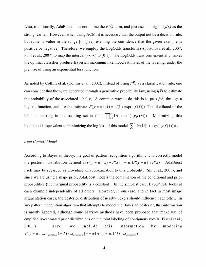
Also, traditionally, AdaBoost does not define the P( ) term, and just uses the sign of f( ) as the

strong learner. However, when using ACM, it is necessary that the output not be a decision rule,

but rather a value in the range [0 1] representing the confidence that the given example is

positive or negative. Therefore, we employ the LogOdds transform (Apostolova et al., 2007;

Pohl et al., 2007) to map the interval (-∞ ∞) to [0 1]. The LogOdds transform essentially makes

the optimal classifier produce Bayesian maximum likelihood estimates of the labeling, under the

premise of using an exponential loss function.

As noted by Collins et al. (Collins et al., 2002), instead of using f( ) as a classification rule, one

can consider that the yi are generated through a generative probability law, using f( ) to estimate

the probability of the associated label yi. A common way to do this is to pass f( ) through a

logistic function, and use the estimate )))(exp(1/(1)|1( xfxyP rr−+=±= The likelihood of the

labels occurring in the training set is then ∏ =−+

N

i i xfy1

)))(exp(1/(1 . Maximizing this

likelihood is equivalent to minimizing the log loss of this model ∑ =−+

N

i i xfy1

))))(exp(1/(1ln( r .

Auto Context Model

According to Bayesian theory, the goal of pattern recognition algorithms is to correctly model

the posterior distribution defined as )(/)1()1|()|1( xPyPyxPxyP ±=±==±= . AdaBoost

itself may be regarded as providing an approximation to this probability (Shi et al., 2005), and

since we are using a shape prior, AdaBoost models the combination of the conditional and prior

probabilities (the marginal probability is a constant). In the simplest case, Bayes’ rule looks at

each example independently of all others. However, in our case, and in fact in most image

segmentation cases, the posterior distribution of nearby voxels should influence each other. In

any pattern recognition algorithm that attempts to model the Bayesian posterior, this information

is mostly ignored, although some Markov methods have been proposed that make use of

empirically-estimated prior distributions on the joint labeling of contiguous voxels (Fischl et al.,

2 0 0 1 ) . H e r e , w e i n c l u d e t h i s i n f o r m a t i o n b y m o d e l i n g

),(/)1()1|,(),|1( neighborsneighborsneighbors xxPyPyxxPxxyP ±=±==±= .

15

ACM attempts to model the above distribution iteratively; a description is given in Figure 2.

Figure 2: An overview of the auto context model.

In our context, H is the cascade of AdaBoosts without the final binary classification step. In

order to improve ACM, instead of starting P1 with a uniform distribution, we instead start with

our shape prior. Also, in order to give more information about the classifications of neighboring

voxels, when running AdaBoost inside of ACM, we included neighborhood features defined on

Pt. Specifically we included the same Haar, curvature, gradient, mean, and standard deviation

filters on the posterior map as we do on the images.

We can prove that for each iteration of ACM, the error is monotonically decreasing. Define the

error of the classification algorithm (in our case a cascade of AdaBoosts) at iteration t to be _t,

we then prove that 1−≤ tt εε . First, we define )|( iit xyp to be the probability change associated

with iteration t of ACM. Next, since Pt-1 includes all previous iterations of ACM, we can write

∑ = −− −=N

i itt yiP1 11 )(loglogε and ∑ = −−=

N

i tiitt iPxyp1 1 ))(,|(loglogε . In the trivial case,

ittiit yiPiPxyp )())(,|( 11 −− = by simply choosing pt to be a uniform distribution. However, since

it has been shown that AdaBoost decreases the error at every iteration, it must choose weak

learners that decrease pt, so therefore 1−≤ tt εε .

Segmentation Overview

16

When implementing our method there are a number of parameters that must be set, but very few

that need to be tweaked. We used approximately 18,000 features in our feature pool. This

includes both features based on the images, and those based on the posterior maps from ACM.

We chose to run each AdaBoost for 200 iterations, obtaining 200 weak learners per AdaBoost

cascade node, a cascade depth of two nodes, and five ACM iterations. This leads to running ten

iterations of AdaBoost during the training phase. Overall, training takes about twelve hours.

Even so, testing is very short, taking less than one minute to segment the hippocampus on a new

brain image.

It is also of interest to note which features AdaBoost chose in order to obtain insight into

the segmentation process. During the first iteration of ACM, AdaBoost chose mostly

features based on the Haar filter and based on the tissue classified image (i.e., binary maps

of gray and white matter and CSF). Later iterations of ACM choose mostly Haar filter

outputs and mean filter outputs based on the previously selected posterior distribution,

which means that neighboring voxels are influencing each other, as is to be expected.

These features are not totally independent, since most are based on the same underlying

image intensities; however each adds some classification ability to the final decision rule.

An advantage of this approach is that the algorithm does not have to rely on the same small

subset of features when trained on different training sets, and can select different features

when trained on different examples, if they are optimal. As with other boosting methods, it

is not expected or even desirable that the same feature sets be recovered when analyzing

images from different sources, and it is not expected that each of the features used has good

classification ability in its own right; in fact, any boosting method uses so-called ‘weak

learners’, with individual classification performance only slightly better than chance, and

combines them effectively using the boosting strategy.

Results:

When validating a machine learning approach it is essential to examine error metrics on

both the training and testing sets. A test set independent of the training set is vital in

machine learning, in order to show the effectiveness of a classifier on data totally withheld

17

from the training set. Since we used 21 hand-labeled brains to train the algorithm, we

employed a leave-one-out analysis to guarantee a separation between the training and

testing sets. In order to put our error metrics in context and decide whether they were

acceptable for the application, we had a second independent expert rater trace the same 21

brains. We were then able to create a triangle of comparisons as shown in Figure 3Figure

3, in which the algorithm’s segmentations can be compared with those of the human rater

who trained the algorithm (rater 1; A.G.) and with those of an independent rater (rater 2;

C.A.) who did not train the algorithm.

Figure 3: A schematic description of the comparisons performed. For all of the tests performed in this paper, training

was performed on rater 1’s tracings.

In order to show agreement with a human expert not involved with training the algorithm,

we only trained our algorithm on manual segmentations from rater 1 and were still able to

achieve good segmentation results that agreed well with rater 2’s manual tracings. We

emphasize that the validation against rater 1 is also an independent validation in the sense

that our algorithm was classifying images that it was not trained on (i.e. a leave-one-out

approach).

Secondly, we further validated our approach using volumetric results of three kinds. We

hypothesized that hippocampal volume would decrease as the disease progresses further,

and verified this by comparing mean volumes in groups of controls, MCI subjects, and AD

patients. We also examined whether, in the full sample, hippocampal volume was

correlated with clinical measurements of cognitive impairment; encouragingly, we found

Rater 1 Rater 2

Our algorithm

18

that measures from our segmentations correlated more strongly with cognition, in the

hippocampus, than measures from a popular technique for quantification of brain atrophy,

tensor-based morphometry, which is closely related to voxel-based morphometry.

Finally, since longitudinal follow-up scans were available for the individuals tested in this

paper, we used scans taken six months later to assess the longitudinal stability of the

segmentations of the same subject. We showed that the amount of hippocampal volume

change was consistent with prior reports in the literature.

Error Metrics

To assess our segmentations’ performance, we first define a number of error metrics based on the

following definitions: A, the ground truth segmentation, and B, the testing segmentation.

Additionally, we define d(a,b) as the Euclidean distance between points a and b.

• Precision BBA∩

=

• Recall ABA∩

=

• Relative Overlap BABA

∪∩

=

• Similarity Index

+∩

=

2BABA

• ))),(((minmax1 badH BbAa ∈∈=

• ))),(((minmax2 abdH AaBb ∈∈=

• Hausdorff 2

21 HH +=

• Mean ))),(((minavg badBbAa ∈∈=

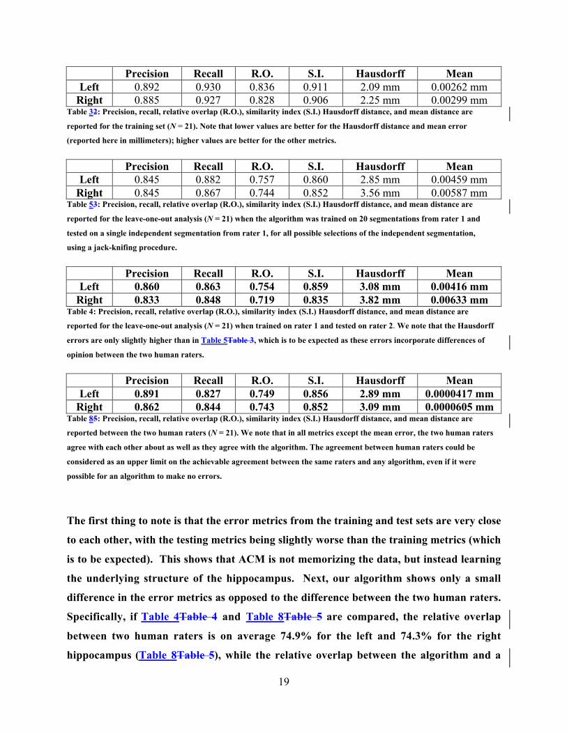
First, Table 3Table 2 presents our segmentation performance on the training set. For this

analysis, we used all 21 brains as training data, and tested on all 21 brains. These

performance results on the training set represent an upper bound for the expected

accuracy on the testing set. Next, we used our leave-one-out approach to obtain testing

metrics comparing our results to rater 1 (leg “b” in Figure 3Figure 3), shown in Table

5Table 3. Table 4 compares our method with rater 2 (leg “c” in Figure 3Figure 3), again

using the leave-one-out technique. Finally, we compared the two human raters directly

with one another (leg “a” in Figure 3Figure 3) in Table 8Table 5.

19

Precision Recall R.O. S.I. Hausdorff MeanLeft 0.892 0.930 0.836 0.911 2.09 mm 0.00262 mm

Right 0.885 0.927 0.828 0.906 2.25 mm 0.00299 mmTable 32: Precision, recall, relative overlap (R.O.), similarity index (S.I.) Hausdorff distance, and mean distance are

reported for the training set (N = 21). Note that lower values are better for the Hausdorff distance and mean error

(reported here in millimeters); higher values are better for the other metrics.



reported for the leave-one-out analysis (N = 21) when the algorithm was trained on 20 segmentations from rater 1 and

tested on a single independent segmentation from rater 1, for all possible selections of the independent segmentation,

using a jack-knifing procedure.



reported for the leave-one-out analysis (N = 21) when trained on rater 1 and tested on rater 2. We note that the Hausdorff

errors are only slightly higher than in Table 5Table 3, which is to be expected as these errors incorporate differences of

opinion between the two human raters.



reported between the two human raters (N = 21). We note that in all metrics except the mean error, the two human raters

agree with each other about as well as they agree with the algorithm. The agreement between human raters could be

considered as an upper limit on the achievable agreement between the same raters and any algorithm, even if it were

possible for an algorithm to make no errors.

The first thing to note is that the error metrics from the training and test sets are very close

to each other, with the testing metrics being slightly worse than the training metrics (which

is to be expected). This shows that ACM is not memorizing the data, but instead learning

the underlying structure of the hippocampus. Next, our algorithm shows only a small

difference in the error metrics as opposed to the difference between the two human raters.

Specifically, if Table 4Table 4 and Table 8Table 5 are compared, the relative overlap

between two human raters is on average 74.9% for the left and 74.3% for the right

hippocampus (Table 8Table 5), while the relative overlap between the algorithm and a

20

rater not involved in training it was 75.4% for the left and 71.9% for the right

hippocampus (Table 4Table 4). This shows that the errors in our algorithm are comparable

to the differences between two raters. In terms of precision, the agreement between the two

human raters is about 3% higher than the agreement between the algorithm and the rater

not used to train it, with all values in the 83-89% range. For recall, the algorithm agrees

with the 2nd rater at least as well as the 1st rater agrees with the 2nd rater, with all values in

the 82-86% range. The only metric for which the human raters agree with each other more

than they do with the algorithm is the mean error (see Table 4Table 4 and Table 8Table 5),

but for that metric agreement is very high between all three suggesting that any biases are

very small.

To further compare the performance of our approach with other segmentation methods, in Table

6Table 6 we present error metrics from three other papers that report either fully or semi-

automated hippocampal segmentations. We present these only to show that ours is within the

same range as other automated approaches. Since each study uses a different set of scans, an

exact comparison is not possible.

Recall R.O. S.I.(Powell et al., 2008) (Left: N = 5) 0.82 0.72 0.84(Powell et al., 2008) (Right: N = 5) 0.83 0.74 0.85(Fischl et al., 2002) (Left: N = 134) N.A. ~0.78 N.A.(Fischl et al., 2002) (Right: N = 134) N.A. ~0.80 N.A.(Hogan et al., 2000) (Left: N = 5) N.A. 0.7378 N.A.(Hogan et al., 2000) (Right: N = 5) N.A. 0.7578 N.A.

Table 6: This table reports hippocampal segmentation metrics for other semi- and fully automated approaches. Our

results compare favorably to those reported here. A complete comparison is not possible without testing performance on

the same set of brains.

Volumetric Validation

Figure 5Figure 4 shows an example brain from the test set, with the right and left hippocampi

overlaid in yellow and green. There is good differentiation of the hippocampus from the

surrounding amygdala, overlying CSF, and adjacent white matter, and the traces are spatially

21

smooth, simply connected, and visually resemble manual segmentations by experts. This image

was chosen at random from the test set, and is representative of the segmentation accuracy

obtainable on the test images.

Axial Coronal

Right Sagittal Left Sagittal

Figure 54: Automated segmentation results for an individual from the testing set. Here the right hippocampus is

encircled in yellow, and the left hippocampus in green. Axial, coronal, and two sagittal slices through the hippocampus

show that the hippocampal boundary is captured accurately.

22

Table 8Table 7 shows that the inter-rater r (intraclass correlation) between the two raters’

hippocampal volumes and the volumes obtained from our algorithm’s segmentations are

comparable. Although the inter-rater r is lower when comparing our approach to either

rater versus the difference between the two raters, the intraclass correlation is high, and, as

expected, statistically significant on both sides. For all of the tests in Table 8Table 7, we

trained the algorithm only on segmentations from rater 1, and this is one reason why there

is a slightly higher correlation observed with rater 1 than with rater 2.

Left Right MeanRater 1 – Us 0.740** 0.717** 0.724**Rater 2 – Us 0.694** 0.709** 0.699**

Rater 1 – Rater 2 0.844** 0.857** 0.854**Table 87: Inter-rater r when comparing the three sets of volumes. These volumes were obtained from the leave-one-out

analysis so a realistic testing environment can be observed.

* p < 0.05

** p < 0.01

Next, we present a disease-based validation technique, based on the premise that a

necessary but not sufficient condition for a valid classifier is that it differentiates group

mean hippocampal volumes between AD, MCI and controls. Since it is well-known that

reductions in hippocampal volume are associated with declining cognitive function (Jack et

al., 1999), we showed that our method is accurately capturing known mean volumetric

differences between subgroups of interest with different stages of dementia (controls, MCI,

and AD). Due to the limited sample size (N = 21), we pooled left and right hippocampal

volumes together for some of these results. Volumetric summaries were computed using

the segmentations obtained in the leave-one-out testing analysis.

23

Figure 75: Volumetric analysis for the three different diagnostic groups. The error bars represent standard errors of

the mean. Percent differences are tabulated in Table 10Table 8.

AllNormal-AD 20.32%**

Normal-MCI 4.13%MCI-AD 16.89%*

Table 108: Mean differences in hippocampal volume (as a percentage) are shown for the groups listed in the left column

for all subjects. Even though this is a very small sample (N=21; 7 of each diagnosis), there is a hippocampal volume

reduction associated with declining function, and the group differences are significant even in a sample this small. These

results are shown for validation purposes; a large sample in the future would allow more accurate estimation of deficits

and factors that influence them.

* p < 0.05

** p < 0.01

Figure 7Figure 5 and Table 10Table 8 show that there is a sequential reduction in volume

between controls, MCI, and AD subjects, consistent with many prior studies (Convit et al.,

1997). This shows that the brain MRIs we are working with show the expected profile of

volumetric effects with disease progression, and that the segmentation approach is measuring

hippocampal volumes with low enough methodological error to differentiate the 3 diagnostic

groups, at least at the group level, in a very small sample.

24

Left HP volume Right HP volume Mean HP volumeMMSE 0.423* 0.579** 0.587**

Sum of Boxes CDR -0.369* -0.705** -0.642**Table 129: This table reports the correlations between hippocampal volumes and clinical covariates. A desirable but not

sufficient condition for a hippocampal segmentation approach is that the methodological error is small enough for

correlations to be detected between cognition and hippocampal volume. As expected, correlations are positive between

MMSE scores and hippocampal volume, as higher MMSE scores denote better cognitive performance. Also as expected,

correlations are negative between hippocampal volume and sum-of-boxes CDR, as higher CDR scores denote more severe

impairment.

* p < 0.05

** p < 0.01

Table 12Table 9 shows strong and significant positive correlations between hippocampal

volume and MMSE scores (r = 0.587 for the average of the left and right hippocampal

volumes; p < 0.01), and with sum of boxes CDR scores, for both the left and right, and

mean hippocampal volumes (r = -0.642 for the mean volume, p < 0.01). Correlations are

high (around 0.6) when the average of the left and right hippocampal volumes is measured,

suggesting that the hippocampal volumes explain a significant proportion of the variation

in clinical decline. Although these associations are known, it provides evidence that the

classifier error is low enough to allow their detection in small samples. Each of these values

is significant despite the very small sample size, further confirming that our method is

capable of capturing disease-associated hippocampal degeneration.

In a previous cross-sectional study on the ADNI dataset, we used tensor-based

morphometry (TBM) to analyze brain differences associated with different stages of

disease progression (Hua et al., 2008). TBM is a method based on high-dimensional image

registration, which derives information on regional volumetric differences from a

deformation field that aligns the images. TBM and voxel-based morphometry (VBM

(Ashburner and Friston, 2000)) are closely linked and each measures voxelwise expansion

(or contraction) of the brain as compared to a minimal deformation template, which

represents the mean anatomy of the subjects (Lepore et al., 2007).

25

Voxel-based morphometry (Davatzikos et al., 2001; Good et al., 2001) is a related approach

that modulates the voxel intensity of a set of spatially normalized gray matter maps by the

local expansion factor of a 3D deformation field that aligns each brain to a standard brain

template.

Although TBM has proven useful in quantifying brain atrophy over time in 3D (Leow et

al., 2005a; Studholme et al., 2004; Teipel et al., 2007), in cross-sectional studies TBM can be

less effective for quantifying volumetric differences in small brain regions (such as the

hippocampus) when the ROI is defined on the minimal deformation template.

This is to be expected, as TBM may be considered a rudimentary hippocampal

segmentation approach that works by fluidly deforming a mean anatomical template onto

the target image – the criteria to guide accurate segmentations are typically limited to

measures of agreement in image intensities, such as the mutual information (Leow et al.,

2005b; Viola and Wells, 1995). Table 13Table 10 shows the correlation between

hippocampal volume (as measured with TBM) and MMSE and sum of boxes CDR scores.

Note that none of the correlations is even significant in this small sample, and the measures

compare poorly with those shown in Table 12Table 9. This suggests that our direct

segmentation of hippocampal anatomy via voxel-level classification is better correlated

with cognition than measures we previously obtained using a deformation-based

morphometry method.

Left HP expansion Right HP expansion Mean HP expansionMMSE 0.099 0.143 0.126

Sum of Boxes CDR -0.151 -0.272 -0.153Table 1310: This table reports the correlations between hippocampal volumes estimated using tensor-based morhometry

(as reported (Hua et al., 2008)) and clinical covariates on the hippocampus when using TBM. None of these correlations

has a significant p-value, by contrast with the hippocampal volume measures obtained by our algorithm, which correlate

strongly with cognitive and clinical decline Table 12Table 9.

Longitudinal Validation by Repeat Scanning

26

As a final validation approach, we segmented a set of six-month follow-up scans, acquired

using an identical imaging protocol, for the individuals whose baseline scans were analyzed

in this paper. At the time of writing, six-month follow-up scans were available for 18 of the

21 subjects analyzed in this paper, including 6 AD patients, 5 MCI patients, and 7 control

subjects. Due to the very small sample size (especially in the AD and MCI groups) and

short interval, we present this analysis to show that our algorithm is reproducible, giving

relatively consistent hippocampal volumes over a short interval, when minimal

hippocampal volume loss is expected. Table 15Table 11 shows that there is minimal loss

over 6 months, which is to be expected. We note that this change represents a combination

of biological changes and the methodological errors in segmentation, which derive partly

from the algorithm and partly from the fact that the image acquisition is not perfectly

reproducible. As these sources of methodological error are expected to be small and

additive, the fact that the mean change is near 1.5% for the left and 0% for the right

hippocampus is in line with expectation. Given that some small biological change is also

occurring, this suggests good longitudinal stability for the volume measurements obtained

by our algorithm.

Left HP Right HP Mean HP% Loss -1.47% 0.08% -0.01%

Table 1511: This table reports the % loss of the hippocampus for all 18 subjects that had follow up scans over a 6 month

interval. For both hippocampi (and the mean volume), the mean percent loss is very small. This indicates good

longitudinal reproducibility of our segmentation algorithm. For all of these tests, the p-value is greater than 0.3,

indicating that there is no significant difference between baseline and 6 month follow up hippocampal volumes. For this

test we segmented the follow-up scans using the leave one out analysis so that a separation between training and testing

brains at each time point is maintained. For the mean difference, first we took the mean hippocampal volume of each

subject (average of left and right), then calculated the percent loss for each subject, and then averaged. This is why the

mean loss is not an average of the left loss and right loss.

Discussion:

In this study, we have demonstrated that ACM is an effective method for segmenting the

hippocampus. There were three major findings. First, the agreement between our

algorithm and two different human raters was comparable with their agreement with each

27

other, which is a reasonable target for segmentation accuracy given that even trained

human raters do not entirely agree on the labeling of all hippocampal voxels. Second, we

found that the agreement with a rater not involved with training the algorithm was almost

as good as the agreement with the rater who trained it, suggesting acceptable inter-rater

reliability versus expert human raters. Third, we found that the hippocampal volumes

segmented by our algorithm correlated well with cognitive and clinical ratings of dementia

severity, which is an important characteristic for an automated volume measurement

algorithm. For an algorithm to be useable in a drug trial context for the quantification of

brain atrophy, it is necessary for the automatically measured volumes to replicate known

differences in mean hippocampal volume between AD, MCI, and controls, and it is also

desirable for the measures to be accurate enough to correlate with clinical measures of

disease burden as they did here in a small sample (21 subjects; 7 of each diagnosis). In a

further demonstration of longitudinal stability, we found that the change detected in 6-

month repeat scans was around 0-1.5% for a group of 18 subjects. As this group was

heterogeneous with regard to diagnosis and the time interval small, the intent of the

experiment was merely to show that the mean changes were small, and within the range of

expected biological variation.

This study is representative of several current research efforts that use automated methods to

measure hippocampal atrophy in AD, including large diffeomorphic metric mapping (Csernansky

et al., 2004; Wang et al., 2007), volumetric analysis (Geuze et al., 2005), and fluid registration

(van de Pol et al., 2007). For purposes of comparison with our technique, we computed

hippocampal volume measures from a related technique, known as tensor-based

morphometry (TBM), which estimates anatomical structure volumes from a deformation

transform that re-shapes a mean anatomical template onto each individual scan. Our TBM

measures correlated poorly with cognitive assessments, although clearly in such a small

sample the power to detect such associations is severely limited. Some reasons why TBM

may not be optimal for hippocampal volumetric study are detailed in Hua et al. (2008) and

(Apostolova et al., 2006a; Becker et al., 2006; Frisoni et al., 2006). TBM is typically best for

assessing differences at a scale greater than 3-4 mm (the typical resolution of the spectral

representation used to compute the deformation field) (Hua et al., 2008; Leow et al., 2005a).

28

For smaller-scale effects, direct modeling of the structure, e.g. using surface-based

geometrical methods, may offer additional statistical power to detect sub-regional

differences. Even then, it may not be possible to achieve accurate regional measurements of

atrophy, especially in small regions such as the hippocampus, since that would assume a

locally highly accurate registration. Direct assessments of hippocampal volume by our

ACM algorithm correlated better than TBM did with clinical dementia ratings and MMSE

scores, and explained a substantial proportion of their variance even in this relatively small

sample (r ~ 0.6; p < 0.01; N = 21). Conversely, a relative advantage of TBM, and other

voxel-based mapping approaches, such as voxel-based morphometry, is that they map the

profile of atrophy throughout the brain without the need for explicit segmentation of

anatomical structures. VBM has been widely used in Alzheimer’s disease studies, and does

not rely on an explicit segmentation of hippocampal anatomy in each scan, other than that

which is implied in a voxel-based analysis by aligning scans to a common template. Chetelat

et al. (Chetelat et al., 2005), for example, tracked gray matter loss with VBM in a

longitudinal study of 18 MCI patients. Whitwell and colleagues (Whitwell et al., 2007)

demonstrated the profile of gray matter loss over three years in 63 MCI subjects, and Good

et al. (Good et al., 2002) compared VBM to region-of-interest analysis and showed that they

compared favorably in detecting structural differences in Alzheimer’s disease.

The machine learning approach presented here selects features based on a training set of

expert segmentations, so it may generalize well for segmenting other subcortical structures,

such as the thalamus and basal ganglia. The next step will be to further examine ACM

with AdaBoost by evaluating it on a large sample, and examining its performance on other

subcortical structures.

References:

Apostolova, L.G., Akopyan, G.G., Partiali, N., Steiner, C.A., Dutton, R.A., Hayashi, K.M.,Dinov, I.D., Toga, A.W., Cummings, J.L., Thompson, P.M., 2007. Structural correlates of apathyin Alzheimer's disease. Dement Geriatr Cogn Disord 24, 91-97.Apostolova, L.G., Dinov, I.D., Dutton, R.A., Hayashi, K.M., Toga, A.W., Cummings, J.L.,Thompson, P.M., 2006a. 3D comparison of hippocampal atrophy in amnestic mild cognitiveimpairment and Alzheimer's disease. Brain 129, 2867-2873.

29

Apostolova, L.G., Dutton, R.A., Dinov, I.D., Hayashi, K.M., Toga, A.W., Cummings, J.L.,Thompson, P.M., 2006b. Conversion of mild cognitive impairment to Alzheimer diseasepredicted by hippocampal atrophy maps. Arch Neurol 63, 693-699.Ashburner, J., Friston, K.J., 2000. Voxel-based morphometry--the methods. Neuroimage 11,805-821.Barnes, J., Scahill, R.I., Boyes, R.G., Frost, C., Lewis, E.B., Rossor, C.L., Rossor, M.N., Fox,N.C., 2004. Differentiating AD from aging using semiautomated measurement of hippocampalatrophy rates. Neuroimage 23, 574-581.Becker, J.T., Davis, S.W., Hayashi, K.M., Meltzer, C.C., Toga, A.W., Lopez, O.L., Thompson,P.M., 2006. Three-dimensional patterns of hippocampal atrophy in mild cognitive impairment.Arch Neurol 63, 97-101.Boyes, R.G., Gunter, J., Frost, C., Janke, A.L., Yeatman, T., Hill, T., Dale, A.M., Bernstein, M.,Thompson, P., Weiner, M.W., Schuff, N., Alexander, G., Fox, N.C., Jack, C.R., 2007.Quantitative Analysis of N3 on 3 Tesla Scanners with Multichannel Phased Array Coils.Neuroimage in press.Chetelat, G., Landeau, B., Eustache, F., Mezenge, F., Viader, F., de la Sayette, V., Desgranges,B., Baron, J.C., 2005. Using voxel-based morphometry to map the structural changes associatedwith rapid conversion in MCI: a longitudinal MRI study. Neuroimage 27, 934-946.Cockrell, J.R., Folstein, M.F., 1988. Mini-Mental State Examination (MMSE). PsychopharmacolBull 24, 689-692.Collins, D.L., Neelin, P., Peters, T.M., Evans, A.C., 1994. Automatic 3D intersubject registrationof MR volumetric data in standardized Talairach space. J Comput Assist Tomogr 18, 192-205.Collins, D.L., Schapire, R.E., Singer, Y., 2002. Logistic Regression, AdaBoost and BregmanDistances. Machine Learning 48, 253-285.Convit, A., De Leon, M.J., Tarshish, C., De Santi, S., Tsui, W., Rusinek, H., George, A., 1997.Specific Hippocampal Volume Reductions in Individuals at Risk for Alzheimer's Disease.Neurobiology of Aging 18, 131-138.Crum, W.R., Scahill, R.I., Fox, N.C., 2001. Automated Hippocampal Segmentation by RegionalFluid Registration of Serial MRI: Validation and Application in Alzheimer's Disease.Neuroimage 13, 847-855.Csernansky, J.G., Joshi, S., Wang, L., Haller, J.W., Gado, M., Miller, J.P., Grenander, U., Miller,M.I., 1998. Hippocampal morphometry in schizophrenia by high dimensional brain mapping.Proc Natl Acad Sci U S A 95, 11406-11411.Csernansky, J.G., Wang, L., Joshi, S.C., Ratnanather, J.T., Miller, M.I., 2004. Computationalanatomy and neuropsychiatric disease: probabilistic assessment of variation and statisticalinference of group difference, hemispheric asymmetry, and time-dependent change. Neuroimage23 Suppl 1, S56-68.Davatzikos, C., Genc, A., Xu, D., Resnick, S.M., 2001. Voxel-based morphometry using theRAVENS maps: methods and validation using simulated longitudinal atrophy. Neuroimage 14,1361-1369.Du, A.T., Schuff, N., Amend, D., Laakso, M.P., Hsu, Y.Y., Jagust, W.J., Yaffe, K., Kramer, J.H.,Reed, B., Norman, D., Chui, H.C., Weiner, M.W., 2001. Magnetic resonance imaging of theentorhinal cortex and hippocampus in mild cognitive impairment and Alzheimer's disease. JNeurol Neurosurg Psychiatry 71, 441-447.Duda, D., Hart, P., Stork, D., 2001. Pattern Classification, 2nd ed. Wiley-Interscience.

30

Fischl, B., Salat, D.H., Busa, E., Albert, M., Dieterich, M., Haselgrove, C., van der Kouwe, A.,Killiany, R., Kennedy, D., Klaveness, S., Montillo, A., Makris, N., Rosen, B., Dale, A.M., 2002.Whole brain segmentation: automated labeling of neuroanatomical structures in the human brain.Neuron 33, 341-355.Folstein, M.F., Folstein, S.E., McHugh, P.R., 1975. "Mini-mental state". A practical method forgrading the cognitive state of patients for the clinician. J Psychiatr Res 12, 189-198.Freund, Y., Schapire, R.E., 1997. A decision-theoretic generalization of online learning and anapplication to boosting. J Comput Sys Sci. 55, 119-139.Friedman, J., Hastie, T., Tibshirani, R., 2000. Additive logistic regression: a statistical view ofboosting (With discussion and a rejoinder by the authors). Annals of Statistics 28, 337-407.Frisoni, G.B., Sabattoli, F., Lee, A.D., Dutton, R.A., Toga, A.W., Thompson, P.M., 2006. In vivoneuropathology of the hippocampal formation in AD: a radial mapping MR-based study.Neuroimage 32, 104-110.Geuze, E., Vermetten, E., Bremner, J.D., 2005. MR-based in vivo hippocampal volumetrics: 2.Findings in neuropsychiatric disorders. Mol Psychiatry 10, 160-184.Good, C.D., Johnsrude, I.S., Ashburner, J., Henson, R.N., Friston, K.J., Frackowiak, R.S., 2001.A voxel-based morphometric study of ageing in 465 normal adult human brains. Neuroimage 14,21-36.Good, C.D., Scahill, R.I., Fox, N.C., Ashburner, J., Friston, K.J., Chan, D., Crum, W.R., Rossor,M.N., Frackowiak, R.S., 2002. Automatic differentiation of anatomical patterns in the humanbrain: validation with studies of degenerative dementias. Neuroimage 17, 29-46.Gunter, J., Bernstein, M., Borowski, B., Felmlee, J., Blezek, D., Mallozzi, R., 2006. Validationtesting of the MRI calibration phantom for the Alzheimer's Disease Neuroimaging InitiativeStudy. ISMRM 14th Scientific Meeting and Exhibition.Hoffgen, K.U., Simon, H.U., 1992. Robust trainability of single neurons. Proceedings of the fifthannual workshop on Computational learning theory. Association for Computing Machinery,Pittsburgh, Pennsylvania, United States, pp. 428-439.Hogan, R.E., Mark, K.E., Wang, L., Joshi, S., Miller, M.I., Bucholz, R.D., 2000. Mesialtemporal sclerosis and temporal lobe epilepsy: MR imaging deformation-based segmentation ofthe hippocampus in five patients. Radiology 216, 291-297.Hua, X., Leow, A.D., Lee, S., Klunder, A.D., Toga, A.W., Lepore, N., Chou, Y.Y., Brun, C.,Chiang, M.C., Barysheva, M., Jack, C.R., Jr., Bernstein, M.A., Britson, P.J., Ward, C.P.,Whitwell, J.L., Borowski, B., Fleisher, A.S., Fox, N.C., Boyes, R.G., Barnes, J., Harvey, D.,Kornak, J., Schuff, N., Boreta, L., Alexander, G.E., Weiner, M.W., Thompson, P.M.,Alzheimer's Disease Neuroimaging, I., 2008. 3D characterization of brain atrophy in Alzheimer'sdisease and mild cognitive impairment using tensor-based morphometry. Neuroimage.Hughes, C.P., Berg, L., Danziger, W.L., Coben, L.A., Martin, R.L., 1982. A new clinical scalefor the staging of dementia. Br J Psychiatry 140, 566-572.Jack, C., Bernstein, M., Fox, N.C., Thompson, P., Alexander, G., Harvery, D., Borowski, B.,Britson, P., Whitwell, J., Ward, C., Dale, A., Felmlee, J., Gunter, J., Hill, D., Killiany, R.,Schuff, N., Fox-Bosetti, S., Lin, C., Studholme, C., DeCarli, C., Krueger, G., Ward, H., Metzger,G., Scott, E., Mallozzi, R., Blezek, D., Levy, J., Debbins, J., Fleisher, A., Albert, M., Green, R.,Bartzokis, G., Glover, G., Mugler, J., Weiner, M.W., 2007. The Alzheimer's DiseaseNeuroimaging Initiative (ADNI): The MR Imaging Protocol. Journal of MRI in press.

31

Jack, C.R., Jr., Petersen, R.C., Xu, Y.C., O'Brien, P.C., Smith, G.E., Ivnik, R.J., Boeve, B.F.,Waring, S.C., Tangalos, E.G., Kokmen, E., 1999. Prediction of AD with MRI-basedhippocampal volume in mild cognitive impairment. Neurology 52, 1397-1403.Jorm, A.F., Korten, A.E., Henderson, A.S., 1987. The prevalence of dementia: a quantitativeintegration of the literature. Acta Psychiatr Scand 76, 465-479.Jovicich, J., Czanner, S., Greve, D., Haley, E., van der Kouwe, A., Gollub, R., Kennedy, D.,Schmitt, F., Brown, G., Macfall, J., Fischl, B., Dale, A., 2006. Reliability in multi-site structuralMRI studies: effects of gradient non-linearity correction on phantom and human data.Neuroimage 30, 436-443.Kantarci, K., Jack, C.R., Jr., 2003. Neuroimaging in Alzheimer disease: an evidence-basedreview. Neuroimaging Clin N Am 13, 197-209.Leow, A., Huang, S.C., Geng, A., Becker, J., Davis, S., Toga, A., Thompson, P., 2005a. Inverseconsistent mapping in 3D deformable image registration: its construction and statisticalproperties. Inf Process Med Imaging 19, 493-503.Leow, A., Yu, C.L., Lee, S.J., Huang, S.C., Protas, H., Nicolson, R., Hayashi, K.M., Toga, A.W.,Thompson, P.M., 2005b. Brain structural mapping using a novel hybrid implicit/explicitframework based on the level-set method. Neuroimage 24, 910-927.Leow, A.D., Klunder, A.D., Jack, C.R., Jr., Toga, A.W., Dale, A.M., Bernstein, M.A., Britson,P.J., Gunter, J.L., Ward, C.P., Whitwell, J.L., Borowski, B.J., Fleisher, A.S., Fox, N.C., Harvey,D., Kornak, J., Schuff, N., Studholme, C., Alexander, G.E., Weiner, M.W., Thompson, P.M.,2006. Longitudinal stability of MRI for mapping brain change using tensor-based morphometry.Neuroimage 31, 627-640.Lepore, N., Brun, C., Pennec, X., Chou, Y.Y., Lopez, O.L., Aizenstein, H.J., Becker, J.T., Toga,A.W., Thompson, P.M., 2007. Mean template for tensor-based morphometry using deformationtensors. Med Image Comput Comput Assist Interv Int Conf Med Image Comput Comput AssistInterv 10, 826-833.Mazziotta, J., Toga, A., Evans, A., Fox, P., Lancaster, J., Zilles, K., Woods, R., Paus, T.,Simpson, G., Pike, B., Holmes, C., Collins, L., Thompson, P., MacDonald, D., Iacoboni, M.,Schormann, T., Amunts, K., Palomero-Gallagher, N., Geyer, S., Parsons, L., Narr, K., Kabani,N., Le Goualher, G., Boomsma, D., Cannon, T., Kawashima, R., Mazoyer, B., 2001. Aprobabilistic atlas and reference system for the human brain: International Consortium for BrainMapping (ICBM). Philos Trans R Soc Lond B Biol Sci 356, 1293-1322.McKhann, G., Drachman, D., Folstein, M., Katzman, R., Price, D., Stadlan, E.M., 1984. Clinicaldiagnosis of Alzheimer's disease: report of the NINCDS-ADRDA Work Group under theauspices of Department of Health and Human Services Task Force on Alzheimer's Disease.Neurology 34, 939-944.Morra, J., Tu, Z., Apostolova, L.G., Green, A., Toga, A., Thompson, P., 2007. Comparison ofAdaBoost and support vector machines for detecting Alzheimer’s disease through automatedhippocampal segmentation. IEEE Trans Med Imaging submitted.Morris, J.C., 1993. The Clinical Dementia Rating (CDR): current version and scoring rules.Neurology 43, 2412-2414.Mueller, S.G., Weiner, M.W., Thal, L.J., Petersen, R.C., Jack, C., Jagust, W., Trojanowski, J.Q.,Toga, A.W., Beckett, L., 2005a. The Alzheimer's disease neuroimaging initiative. NeuroimagingClin N Am 15, 869-877, xi-xii.

32

Mueller, S.G., Weiner, M.W., Thal, L.J., Petersen, R.C., Jack, C.R., Jagust, W., Trojanowski,J.Q., Toga, A.W., Beckett, L., 2005b. Ways toward an early diagnosis in Alzheimer's disease:The Alzheimer's Disease Neuroimaging Initiative (ADNI). Alzheimers Dement 1, 55-66.Petersen, R.C., 2000. Aging, Mild Cognitive Impairment, and Alzheimer's Disease. NeurologicClinics 18, 789-805.Petersen, R.C., Doody, R., Kurz, A., Mohs, R.C., Morris, J.C., Rabins, P.V., Ritchie, K., Rossor,M., Thal, L., Winblad, B., 2001. Current concepts in mild cognitive impairment. Arch Neurol 58,1985-1992.Petersen, R.C., Smith, G.E., Waring, S.C., Ivnik, R.J., Tangalos, E.G., Kokmen, E., 1999. Mildcognitive impairment: clinical characterization and outcome. Arch Neurol 56, 303-308.Pohl, K.M., Kikinis, R., Wells, W.M., 2007. Active mean fields: solving the mean fieldapproximation in the level set framework. Inf Process Med Imaging 20, 26-37.Powell, S., Magnotta, V.A., Johnson, H., Jammalamadaka, V.K., Pierson, R., Andreasen, N.C.,2008. Registration and machine learning-based automated segmentation of subcortical andcerebellar brain structures. Neuroimage 39, 238-247.Quddus, A., Fieguth, P., Basir, O., 2005. Adaboost and Support Vector Machines for WhiteMatter Lesion Segmentation in MR Images. Conf Proc IEEE Eng Med Biol Soc 1, 463-466.Shattuck, D.W., Sandor-Leahy, S.R., Schaper, K.A., Rottenberg, D.A., Leahy, R.M., 2001.Magnetic resonance image tissue classification using a partial volume model. Neuroimage 13,856-876.Shi, Y., Bobick, A., Essa, I., 2005. A Bayesian view of boosting and its extensions. GeorgiaTech's Institutional Repository. Georgia Institue of Technology.Sled, J.G., Zijdenbos, A.P., Evans, A.C., 1998. A nonparametric method for automatic correctionof intensity nonuniformity in MRI data. IEEE Trans Med Imaging 17, 87-97.Studholme, C., Cardenas, V., Blumenfeld, R., Schuff, N., Rosen, H.J., Miller, B., Weiner, M.,2004. Deformation tensor morphometry of semantic dementia with quantitative validation.Neuroimage 21, 1387-1398.Teipel, S.J., Born, C., Ewers, M., Bokde, A.L., Reiser, M.F., Moller, H.J., Hampel, H., 2007.Multivariate deformation-based analysis of brain atrophy to predict Alzheimer's disease in mildcognitive impairment. Neuroimage 38, 13-24.Thompson, P.M., Hayashi, K.M., De Zubicaray, G.I., Janke, A.L., Rose, S.E., Semple, J., Hong,M.S., Herman, D.H., Gravano, D., Doddrell, D.M., Toga, A.W., 2004. Mapping hippocampaland ventricular change in Alzheimer disease. Neuroimage 22, 1754-1766.Tu, Z., Narr, K., Dinov, I., Dollar, P., Thompson, P., Toga, A., 2007. Brain anatomical structureparsing by hybrid discriminative/generative models. IEEE Trans Med Imaging in press.van de Pol, L.A., Barnes, J., Scahill, R.I., Frost, C., Lewis, E.B., Boyes, R.G., van Schijndel,R.A., Scheltens, P., Fox, N.C., Barkhof, F., 2007. Improved reliability of hippocampal atrophyrate measurement in mild cognitive impairment using fluid registration. Neuroimage 34, 1036-1041.Viola, P., Jones, M.J., 2004. Robust Real-Time Face Detection. International Journal ofComputer Vision 57, 137-154.Viola, P., Wells, W.M., 1995. Alignment by Maximization of Mutual Information. IEEE, 16 -23.Wang, L., Beg, F., Ratnanather, T., Ceritoglu, C., Younes, L., Morris, J.C., Csernansky, J.G.,Miller, M.I., 2007. Large deformation diffeomorphism and momentum based hippocampal shapediscrimination in dementia of the Alzheimer type. IEEE Trans Med Imaging 26, 462-470.

33

Wechsler, D., 1987. Wechsler Memory Scale. Psychological Corp / Harcourt Brace Jovanovich,New York.Whitwell, J.L., Shiung, M.M., Przybelski, S.A., Weigand, S.D., Knopman, D.S., Boeve, B.F.,Petersen, R.C., Jack, C.R., Jr., 2007. MRI patterns of atrophy associated with progression to ADin amnestic mild cognitive impairment. Neurology.Yushkevich, P.A., Piven, J., Hazlett, H.C., Smith, R.G., Ho, S., Gee, J.C., Gerig, G., 2006. User-guided 3D active contour segmentation of anatomical structures: significantly improvedefficiency and reliability. Neuroimage 31, 1116-1128.

34

Figure 1: An overview of the AdaBoost algorithm. 1 is an indicator function, returning 1 if the statement is true and 0otherwise.Figure 1: An overview of the AdaBoost algorithm. 1 is an indicator function, returning 1 if the statement istrue and 0 otherwise.

Figure 2: An overview of the auto context model.Figure 2: An overview of the auto context model.

Figure 3: A schematic description of the comparisons performed. For all of the tests performed in this paper, trainingwas performed on rater 1’s tracings.Figure 3: A schematic description of the comparisons performed. For all of the testsperformed in this paper, training was performed on rater 1’s tracings.

Figure 5: Automated segmentation results for an individual from the testing set. Here the right hippocampus is encircledin yellow, and the left hippocampus in green. Axial, coronal, and two sagittal slices through the hippocampus show thatthe hippocampal boundary is captured accurately.Figure 4: Automated segmentation results for an individual from thetesting set. Here the right hippocampus is encircled in yellow, and the left hippocampus in green. Axial, coronal, and twosagittal slices through the hippocampus show that the hippocampal boundary is captured accurately.

Figure 7: Volumetric analysis for the three different diagnostic groups. The error bars represent standard errors of themean. Percent differences are tabulated in Table 10.Figure 5: Volumetric analysis for the three different diagnosticgroups. The error bars represent standard errors of the mean. Percent differences are tabulated in Table 8.

Table 1: Demographic data and clinical scores are shown for the subjects whose scans were analyzed in this paper. Meansare shown with standard deviations in parentheses. This data is provided to show that our individuals encompassed awide variety of cognitive impairment. Throughout the paper, p-values for group differences were obtained from twosided t-tests.* p < 0.05** p < 0.01Table 1: Demographic data and clinical scores are shown for the subjects whose scans were analyzed in thispaper. Means are shown with standard deviations in parentheses. This data is provided to show that our individualsencompassed a wide variety of cognitive impairment. Throughout the paper, p-values for group differences wereobtained from two sided t-tests.* p < 0.05** p < 0.01

Table 3: Precision, recall, relative overlap (R.O.), similarity index (S.I.) Hausdorff distance, and mean distance arereported for the training set (N = 21). Note that lower values are better for the Hausdorff distance and mean error(reported here in millimeters); higher values are better for the other metrics.Table 2: Precision, recall, relative overlap(R.O.), similarity index (S.I.) Hausdorff distance, and mean distance are reported for the training set (N = 21). Note thatlower values are better for the Hausdorff distance and mean error (reported here in millimeters); higher values are betterfor the other metrics.

Table 5: Precision, recall, relative overlap (R.O.), similarity index (S.I.) Hausdorff distance, and mean distance arereported for the leave-one-out analysis (N = 21) when the algorithm was trained on 20 segmentations from rater 1 andtested on a single independent segmentation from rater 1, for all possible selections of the independent segmentation,using a jack-knifing procedure.Table 3: Precision, recall, relative overlap (R.O.), similarity index (S.I.) Hausdorffdistance, and mean distance are reported for the leave-one-out analysis (N = 21) when the algorithm was trained on 20segmentations from rater 1 and tested on a single independent segmentation from rater 1, for all possible selections of theindependent segmentation, using a jack-knifing procedure.

Table 4: Precision, recall, relative overlap (R.O.), similarity index (S.I.) Hausdorff distance, and mean distance arereported for the leave-one-out analysis (N = 21) when trained on rater 1 and tested on rater 2. We note that the Hausdorfferrors are only slightly higher than in Table 5, which is to be expected as these errors incorporate differences of opinionbetween the two human raters.Table 4: Precision, recall, relative overlap (R.O.), similarity index (S.I.) Hausdorffdistance, and mean distance are reported for the leave-one-out analysis (N = 21) when trained on rater 1 and tested onrater 2. We note that the Hausdorff errors are only slightly higher than in Table 3, which is to be expected as these errorsincorporate differences of opinion between the two human raters.

35

Table 8: Precision, recall, relative overlap (R.O.), similarity index (S.I.) Hausdorff distance, and mean distance arereported between the two human raters (N = 21). We note that in all metrics except the mean error, the two human ratersagree with each other about as well as they agree with the algorithm. The agreement between human raters could beconsidered as an upper limit on the achievable agreement between the same raters and any algorithm, even if it werepossible for an algorithm to make no errors.Table 5: Precision, recall, relative overlap (R.O.), similarity index (S.I.)Hausdorff distance, and mean distance are reported between the two human raters (N = 21). We note that in all metricsexcept the mean error, the two human raters agree with each other about as well as they agree with the algorithm. Theagreement between human raters could be considered as an upper limit on the achievable agreement between the sameraters and any algorithm, even if it were possible for an algorithm to make no errors.

Table 6: This table reports hippocampal segmentation metrics for other semi- and fully automated approaches. Ourresults compare favorably to those reported here. A complete comparison is not possible without testing performance onthe same set of brains.Table 6: This table reports hippocampal segmentation metrics for other semi- and fully automatedapproaches. Our results compare favorably to those reported here. A complete comparison is not possible withouttesting performance on the same set of brains.

Table 8: Inter-rater r when comparing the three sets of volumes. These volumes were obtained from the leave-one-outanalysis so a realistic testing environment can be observed. * p < 0.05** p < 0.01Table 7: Inter-rater r when comparing the three sets of volumes. These volumes were obtained from the leave-one-out analysis so a realistic testing environment can be observed. * p < 0.05** p < 0.01

Table 10: Mean differences in hippocampal volume (as a percentage) are shown for the groups listed in the left columnfor all subjects. Even though this is a very small sample (N=21; 7 of each diagnosis), there is a hippocampal volumereduction associated with declining function, and the group differences are significant even in a sample this small. Theseresults are shown for validation purposes; a large sample in the future would allow more accurate estimation of deficitsand factors that influence them.* p < 0.05** p < 0.01Table 8: Mean differences in hippocampal volume (as a percentage) are shown for the groups listed in theleft column for all subjects. Even though this is a very small sample (N=21; 7 of each diagnosis), there is a hippocampalvolume reduction associated with declining function, and the group differences are significant even in a sample this small.These results are shown for validation purposes; a large sample in the future would allow more accurate estimation ofdeficits and factors that influence them.* p < 0.05** p < 0.01

Table 12: This table reports the correlations between hippocampal volumes and clinical covariates. A desirable but notsufficient condition for a hippocampal segmentation approach is that the methodological error is small enough forcorrelations to be detected between cognition and hippocampal volume. As expected, correlations are positive betweenMMSE scores and hippocampal volume, as higher MMSE scores denote better cognitive performance. Also as expected,correlations are negative between hippocampal volume and sum-of-boxes CDR, as higher CDR scores denote more severeimpairment.* p < 0.05** p < 0.01Table 9: This table reports the correlations between hippocampal volumes and clinical covariates. A desirablebut not sufficient condition for a hippocampal segmentation approach is that the methodological error is small enough forcorrelations to be detected between cognition and hippocampal volume. As expected, correlations are positive betweenMMSE scores and hippocampal volume, as higher MMSE scores denote better cognitive performance. Also as expected,correlations are negative between hippocampal volume and sum-of-boxes CDR, as higher CDR scores denote more severeimpairment.

36

* p < 0.05** p < 0.01

Table 13: This table reports the correlations between hippocampal volumes estimated using tensor-based morhometry (asreported (Hua et al., 2008)) and clinical covariates on the hippocampus when using TBM. None of these correlations has asignificant p-value, by contrast with the hippocampal volume measures obtained by our algorithm, which correlatestrongly with cognitive and clinical decline Table 12.Table 10: This table reports the correlations between hippocampalvolumes estimated using tensor-based morhometry (as reported (Hua et al., 2008)) and clinical covariates on thehippocampus when using TBM. None of these correlations has a significant p-value, by contrast with the hippocampalvolume measures obtained by our algorithm, which correlate strongly with cognitive and clinical decline Table 9.

Table 15: This table reports the % loss of the hippocampus for all 18 subjects that had follow up scans over a 6 monthinterval. For both hippocampi (and the mean volume), the mean percent loss is very small. This indicates goodlongitudinal reproducibility of our segmentation algorithm. For all of these tests, the p-value is greater than 0.3,indicating that there is no significant difference between baseline and 6 month follow up hippocampal volumes. For thistest we segmented the follow-up scans using the leave one out analysis so that a separation between training and testingbrains at each time point is maintained.Table 11: This table reports the % loss of the hippocampus for all 18 subjects thathad follow up scans over a 6 month interval. For both hippocampi (and the mean volume), the mean percent loss is verysmall. This indicates good longitudinal reproducibility of our segmentation algorithm. For all of these tests, the p-value isgreater than 0.3, indicating that there is no significant difference between baseline and 6 month follow up hippocampalvolumes. For this test we segmented the follow-up scans using the leave one out analysis so that a separation betweentraining and testing brains at each time point is maintained.

validation of a fully automated 3d hippocampal...

Documents