validating you io subsystem - new york oracle user...

A Texas Memory Systems Presentation

Validating your IO Subsystem

Coming Out of the Black Box

Mike Ault, Oracle Guru, TMS, Inc.


The Black Box

For most people the IO subsystem for their servers is a black box.

The capacity (as defined in megabytes) is easy to confirm

The performance (defined by input and output operations per second (IOPS) and latency (milliseconds, ms) may be more difficult to determine.

In this paper we will explore different methodologies to obtain the IOPS and latency for your application.


IO Is not a Black Box

We are led to believe that the entire IO

subsystem is out of our hands

The details of the IO subsystem will make

or break your database performance.

Eventually almost all performance issues

are traced to IO issues.


IO is Not a Black Box

Inside Oracle, views such as v$filestat and

v$tempstat provide cumulative information

about IO operations

Using some simple queries you can

determine long term averages for IOPS

and latency for the files in your system.

To get more granular data, tools such as

Statspack and AWR must be used


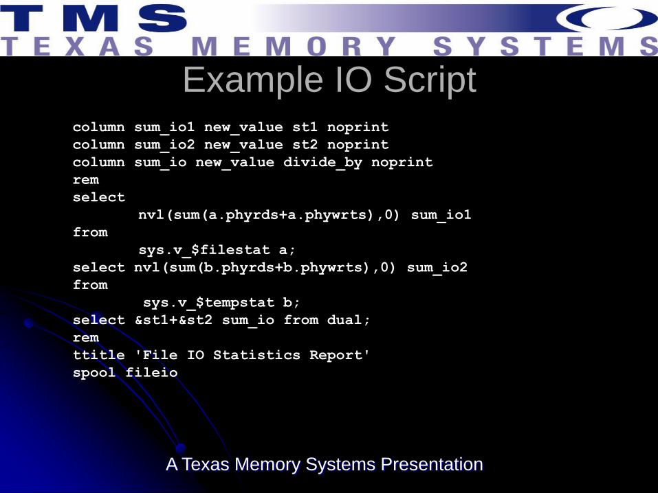
Example IO Script column sum_io1 new_value st1 noprint

column sum_io2 new_value st2 noprint

column sum_io new_value divide_by noprint

rem

select

nvl(sum(a.phyrds+a.phywrts),0) sum_io1

from

sys.v_$filestat a;

select nvl(sum(b.phyrds+b.phywrts),0) sum_io2

from

sys.v_$tempstat b;

select &st1+&st2 sum_io from dual;

rem

ttitle 'File IO Statistics Report'

spool fileio


Example IO Script

select

a.file#,b.name, a.phyrds, a.phywrts,

(100*(a.phyrds+a.phywrts)/&divide_by) Percent,

a.phyblkrd, a.phyblkwrt,

(a.phyblkrd/greatest(a.phyrds,1)) brratio,

(a.phyblkwrt/greatest(a.phywrts,1)) bwratio

from

sys.v_$filestat a, sys.v_$dbfile b

where

a.file#=b.file#

union


Example IO Script

select

c.file#,d.name, c.phyrds, c.phywrts,

(100*(c.phyrds+c.phywrts)/&divide_by) Percent,

c.phyblkrd,

c.phyblkwrt,(c.phyblkrd/greatest(c.phyrds,1)) brratio,

(c.phyblkwrt/greatest(c.phywrts,1)) bwratio

from

sys.v_$tempstat c, sys.v_$tempfile d

where

c.file#=d.file#

order by

1

/


IO Timing Report

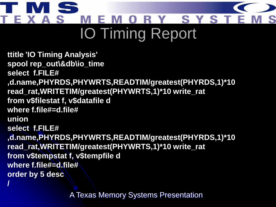
ttitle 'IO Timing Analysis'

spool rep_out\&db\io_time

select f.FILE#

,d.name,PHYRDS,PHYWRTS,READTIM/greatest(PHYRDS,1)*10

read_rat,WRITETIM/greatest(PHYWRTS,1)*10 write_rat

from v$filestat f, v$datafile d

where f.file#=d.file#

union

select f.FILE#

,d.name,PHYRDS,PHYWRTS,READTIM/greatest(PHYRDS,1)*10

read_rat,WRITETIM/greatest(PHYWRTS,1)*10 write_rat

from v$tempstat f, v$tempfile d

where f.file#=d.file#

order by 5 desc

/


What Every IO Subsystem Needs


What Every IO Subsystem Needs

Of course from a purely logical viewpoint the IO subsystem needs to provide three things to the servers:

1. Storage capacity (megabytes, gigabytes, terabytes, etc),

2. Bandwidth (megabytes, gigabytes or terabytes per second), and

3. Low response time (low enough latency for performance) (millisecond or sub-millisecond response).


Where are Storage Systems Going?

Disk based systems have gone from 5000 RPM and 30 or less megabytes to 15K RPM and terabytes in size in the last 20 years.

The first Winchester technology drive I came in contact with had a 90 megabyte capacity (9 times the capacity that the 12 inch platters I was used to had) and was rack mounted, since it weighed over 100 pounds!

Now we have 3 terabyte drives in a 3½ inch form factor.



As information density increased, the

bandwidth of information transfer didn’t

keep up

Most modern disk drives can only

accomplish 2 to 3 times the transfer rate of

their early predecessors, why is this?


HDD Limiting Components


Modern storage systems can deliver hundreds

of thousands of IOPS

You must provide enough disk spindles in the

array to allow this.

For 100,000 IOPS with 300 IOPS per disk you

need 334 disk drives

The IOPS latency would still be from 2-5

milliseconds or greater.

The only way to reduce disk latency to nearer to

the 2 millisecond level is short-stroking.



Short Stroking

Short stroking means only utilizing the

outer, faster, edges of the disk, in fact

usually less than 30% of the total disk

capacity.

Those 334 disks just became 1000 or

more to give 100,000 IOPS at 2

millisecond latency.


Disk Cost $ per GB RAW

$1.00

$10.00

$100.00

$1,000.00

5/24/2002 5/24/2003 5/23/2004 5/23/2005 5/23/2006 5/23/2007 5/22/2008 5/22/2009 5/22/2010 5/22/2011 5/21/2012 5/21/2013

$/GB HDD

$ GB HDD (est)

Expon. ($/GB HDD)


SSD The New Kids SSD technology is the new kid on the block (well,

actually they have been around since the first memory chips).

Costs have fallen to the point where SSD storage using Flash technology is nearly on par with enterprise disk costs with SSD cost per gigabyte falling below $40/gb.

SSD technology using SLC Flash memory chips provides reliable, permanent, and inexpensive storage alternatives to traditional hard drives.

Since each SSD doesn’t require its own motor, actuator and spinning disks, SSD’s price will continue to fall as manufacturing technology and supply-and-demand allows.


The Future

SSD

High

Performance

Disks

Archival Storage


SSD: The Future

Operational costs (electric, cooling) for SSD technology are lower than the costs for hard disk based technology.

With the smaller footprint per usable capacity you have a combination that sounds a death knoll for disk in the high performance end of the storage spectrum.

By the year 2012 or sooner, SSDs will be less expensive than enterprise level disks at dollars (or Euros) per gigabyte.

When a single 3-U chassis full of SSDs can replace over 1000 disks and nearly match the price, it is clear that SSDs will be taking over storage.


Numbers Don’t Lie


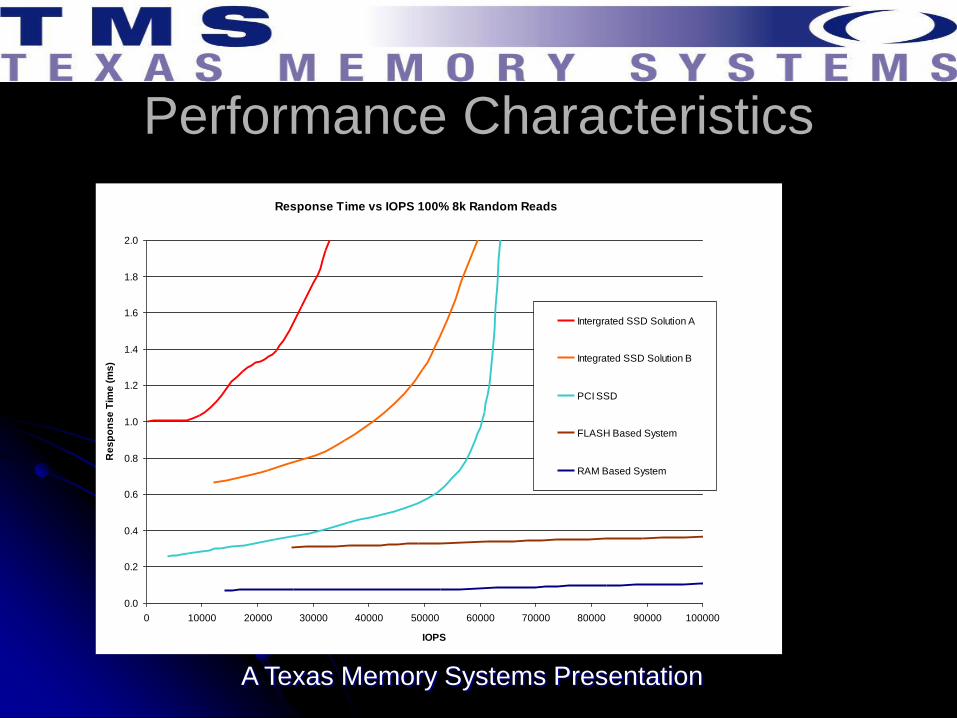
Performance Characteristics

Response Time vs IOPS 100% 8k Random Reads

0.0

0.2

0.4

0.6

0.8

1.0

1.2

1.4

1.6

1.8

2.0

0 10000 20000 30000 40000 50000 60000 70000 80000 90000 100000

IOPS

Re

sp

on

se

Tim

e (

ms

)

Intergrated SSD Solution A

Integrated SSD Solution B

PCI SSD

FLASH Based System

RAM Based System


Types of IO Subsystems

There are essentially three types of IO

subsystems, these are:

1. SAN – Storage area network,

2. NAS – Network attached storage, and

3. DAS – Direct attached storage.


Basic Interfaces SAN

SCSI Fibre Channel/InfiniBand

SATA Fibre Channel/InfiniBand

SSD Fibre Channel/InfiniBand

NAS Ethernet

iSCSI

SATA

DAS ATA

SATA

SCSI

PCIe


IO System Issues

Capacity

Bandwidth

Latency


Capacity

Depending on performance, you decide how

much of each disk can be used, subtract the rest

and then divide the needed capacity by the

amount available on each disk.

Use the proper multiplier for concurrency and

RAID level to determine the number of physical

platters required.

The number of disks needed for concurrency of

access depends on queuing theory.


Bandwidth

Bandwidth is fairly easy to determine if you have the maximum IOPS needed for your application and the size of each IO.

Once you know how many gigabytes or megabytes per second are needed, then the decision comes down to the number and type of host bus adapters (HBA) needed to meet the bandwidth requirement.


If all you need is Bandwidth…


Latency

Don’t try to tie latency and IOPS together.

IOPS are easy to get even with

horrendous latency.

With some disk based systems as latency

increases, so will IOPS until bandwidth is

saturated


Latency IOPS per Latency 6 Disks

0

100

200

300

400

500

600

700

800

900

1000

1100

1200

1300

1400

1500

1600

11 15 18 23 28 35 40 46 49 54 59 65 71 75 78 87 92 93 102

Latency

IOP

S

Max IopsMax MBPSMax PMBPS


Latency

lower latency will result in higher IOPS, but low latency is not required to get higher IOPS.

As long as bandwidth is available you can add disks to a SAN and increase IOPS, however, each IO will still be between 2-5 ms or worse in latency!

The lower the latency the better the chance that a transaction will take a shorter period of time to complete, thus response time is reduced and performance increases.

In a heavily cached SAN you can see 1 millisecond or better response times, until the cache is saturated.

Once the cache is saturated performance returns to disk based latency values.


Latency

To break the 1 ms barrier you need to look at

either DDR or Flash based SSD solutions.

In a DDR based SSD, latencies will be less than

20 microseconds (.02 ms) and in a Flash based

SSD the latency should be between .080-.250

ms.

Most enterprise level SSD systems will use a

combination of DDR buffers and Flash for

permanent storage.


Benchmarking Your Current IO

To accurately model databases we must

be able to control two parts of the

environment:

1. User load

2. Transaction mix


Use of Tools

To completely control both the users and

the transaction load utilize benchmarking

tools.

In the next section of this paper we look at

the benchmark tools you can utilize to

perform accurate trend analysis and

prediction.


Trend identification with

benchmark tools If all that benchmarking tools did were standard canned

benchmarks, they would be of limited use for trend analysis.

Benchmark Factory from Quest provide utilities that allow the reading of trace files from Oracle and the entry of SQL statements to test transactions.

The tools should allow for the specification of multiple user scenarios so that insert, update, delete as well as select transactions can be modeled.

Loadrunner and Mercury capture keystrokes and then use multiple users to provide for stress testing.


Performance Review Using

Oracle SQL Replay in Oracle10g

Real application testing or database replay in Oracle11g.

SQL Replay allows the capture and replay of a single set of SQL statements and these can then be used for a one-time run to perform regression testing in a before and after changes scenario.

Database replay in Oracle11g allows capturing all or portions of a running database’s transactions and then replaying those transactions in another system.

Both of the Oracle based tools only do regression tests.


Other Oracle Tools

Other Tools from Oracle are Statspack

and the automated workload repository

(AWR).

These are performance monitoring tools

but can be used to perform before and

after checks on a system providing the

identical workload can be run at will.


Profiling an Oracle Storage

Workload Oracle keeps storage statistics that are

accessible from AWR or Statspack

Finding the three storage characteristics

(bandwidth, latency, queue) and the two

workload characteristics (average transfer size,

application queue) is a straightforward exercise.

The website www.statspackanalyzer.com

automates this process and outputs the storage

profile for an AWR/Statspack report.

http://www.statspackanalyzer.com/


IOPS, Bandwidth, and Average

IO Size - Oracle 10g Simply collect an AWR report for a busy period for the

database, go to the Instance Activity Stats and look for

the per second values for the following counters:

physical read total IO requests – Total read (input) requests

per second

physical read total bytes – Read Bandwidth

physical write total IO requests – Total write (output)

requests per second

physical write total bytes – Write bandwidth


AWR Example Instance Activity Stats DB/Inst: RAMSAN/ramsan Snaps: 22-23

Statistic Total per Second per Trans

--------------------------------- ------------------ -------------- -----------

physical read IO requests 302,759 4,805.7 20,183.9

physical read bytes 35,364,380,672 561,339,375.8 ###########

physical read total IO requests 302,945 4,808.7 20,196.3

physical read total bytes 35,367,449,600 561,388,088.9 ###########

physical read total multi block r 292,958 4,650.1 19,530.5

…

physical reads prefetch warmup 0 0.0 0.0

physical write IO requests 484 7.7 32.3

physical write bytes 5,398,528 85,690.9 359,901.9

physical write total IO requests 615 9.8 41.0


AWR Example From this example you can see that the IO traffic is

almost exclusively reads: ~560 MB/s bandwidth and ~4,800 IOPS.

Using a variant of one of the formulas presented above, the average size per IO can be calculated as 116 KB per IO.

The queue depth for this traffic can’t be deduced from these measurements alone, because it is dependent on the response time of the storage device (where device latency, device bandwidth, and the maximum device queue are factors).

Response time is available from another section of the report which is unchanged from earlier Oracle 8 and 9 Statspack reports.


Bandwidth, IOPS, and Average IO Size

A single Statspack report from an Oracle 9

database will be used for the remainder of

this paper so data from various sections

can be compared, Statspack and AWR

reports from versions 9, 10 and 11 are

similar and this information will apply to all

versions.


Bandwidth Load Profile

~~~~~~~~~~~~ Per Second Per Transaction

--------------- ---------------

Redo size: 17,007.41 16,619.62

Logical reads: 351,501.17 343,486.49

Block changes: 125.08 122.23

Physical reads: 11,140.07 10,886.06

Physical writes: 1,309.27 1,279.41

User calls: 7,665.49 7,490.70

Parses: 14.34 14.02

Hard parses: 4.36 4.26

Sorts: 2.85 2.78

Logons: 0.17 0.17

Executes: 22.41 21.90

Transactions: 1.02


Bandwidth

These are recorded as database blocks per second rather than IOs per second.

A single large read of 16 sequential database blocks has the same count as 16 single block reads of random locations.

Since the storage system will see this as one large IO request in the first case and 16 IO requests in the second, the IOPS can’t be determined from this data.

To determine the bandwidth the database block size needs to be known.

The standard database block size is recorded in the header for the report.


Bandwidth

STATSPACK report for

DB Name DB Id Instance Inst Num Release Cluster Host

------------ ----------- ------------ -------- ----------- ------- -------

MTR 3056795493 MTR 1 9.2.0.6.0 NO Oraprod

Snap Id Snap Time Sessions Curs/Sess Comment

------- ------------------ -------- --------- ----------------

Begin Snap: 25867 13-Dec-06 11:45:01 31 .9

End Snap: 25868 13-Dec-06 12:00:01 127 7.5

Elapsed: 15.00 (mins)

Cache Sizes (end)

~~~~~~~~~~~~~~~~~

Buffer Cache: 7,168M Std Block Size: 8K

Shared Pool Size: 400M Log Buffer: 2,048K


Bandwidth

The IO profile for this database is mainly reads, and is ~12,500 database blocks per second.

For this database the block size is 8 KB. The bandwidth of the database is the physical reads and physical writes multiplied by the blocksize

In this case about 100 MB/s (90 MB/s reads and 10 MB/s writes).


IOPS and Response Time The IOPS, bandwidth, and response time can be found

from the Tablespace IO Statistics section

If you have more than one tier of storage available you can use the Tablespace IO Stats to determine the table spaces that can benefit the most from faster storage.

Take the Av Reads/s multiplied by the Av Rd (ms) and save this data. This is the amount of time spent waiting (Tw) on IO for a tablespace.

Next find the used capacity of each tablespace. (DBA_EXTENTS) Select tablespace_name, sum(bytes)/(1024*1024) meg from

dba_extents;

The tablespaces with the highest amount of wait time per used capacity are the top candidates for higher performance storage. (Tw/meg)


IOPS and Tw/mb The Av Reads/s and the Av Writes/s for each tablespace

are shown; sum across all tablespaces to get the IOPS.

The 10,000 IOPS is predominantly reads.

The average read response time is Av Rd(ms) for each tablespace.

For overall read response time, use the weighted average response time across all tablespaces using Av reads/s for the weighting. For this database it is ~5.5 milliseconds.

The write response time for the tablespaces isn’t directly measureable because the DBWR process is a background process.

For simplicity take the read response time to be the storage response time because writes in Oracle are either storage array cache friendly (logs) or background processes


Storage Workload

The storage workload for this database is now

fully defined:

Predominantly reads

100 MB/s

10,000 IOPS

5.5 ms response time

The average request size and queue for the profile

can be found using the formulas provided earlier:

Application queue depth: ~55

Average request size: 10 KB


Benchmarking For many databases, exact test environment is next to

impossible.

Incorrect conclusions can be drawn by a test environment when loads don’t compare to production.

Even if hardware is available for testing, the ability to generate a heavy user work load isn’t a possibility.

If an application-level test is performed, it is critically important to measure the storage workload of the test environment and compare it to what was measured in production before beginning any software or hardware optimization changes.

If there is a big difference in the storage profile, then the test environment is not a valid proxy for production.


Benchmarking

If a dedicated enterprise storage array with a

large cache is available in a test environment,

the response time could be quite good

If in production the array supports a wide

number of applications and the array cache

cannot be considered a dedicated resource,

response time of the array will be wildly different.

Applications that perform wonderfully in test may

fail miserably in production.


Benchmarking

The storage profile for an application is

used to create a synthetic environment

This is be helpful to evaluate different

storage devices after storage has been

found to be the bottleneck for a database.


Storage Benchmarking Tools

IOmeter

Oracle’s IO benchmarking utility: ORION

Oracle11g CALIBRATE_IO

These benchmarking tools don’t actually process any of the data that is sent or received to a storage array so the processing power requirements of the server running the test are slight.

As many storage vendors will provide equipment free of charge for a demo or trial period for prospective customers, the costs associated with running these tests are minimal.


IOMeter

IOmeter is a free tool available at www.iometer.org that can be used to create virtually any I/O workload desired.

It is a very powerful tool that can be a bit intimidating on the first use but is easy to use once the main control points are identified.

It is easiest to use from a Windows platform.

http://www.iometer.org/


IOMeter Setup


IOMeter Setup

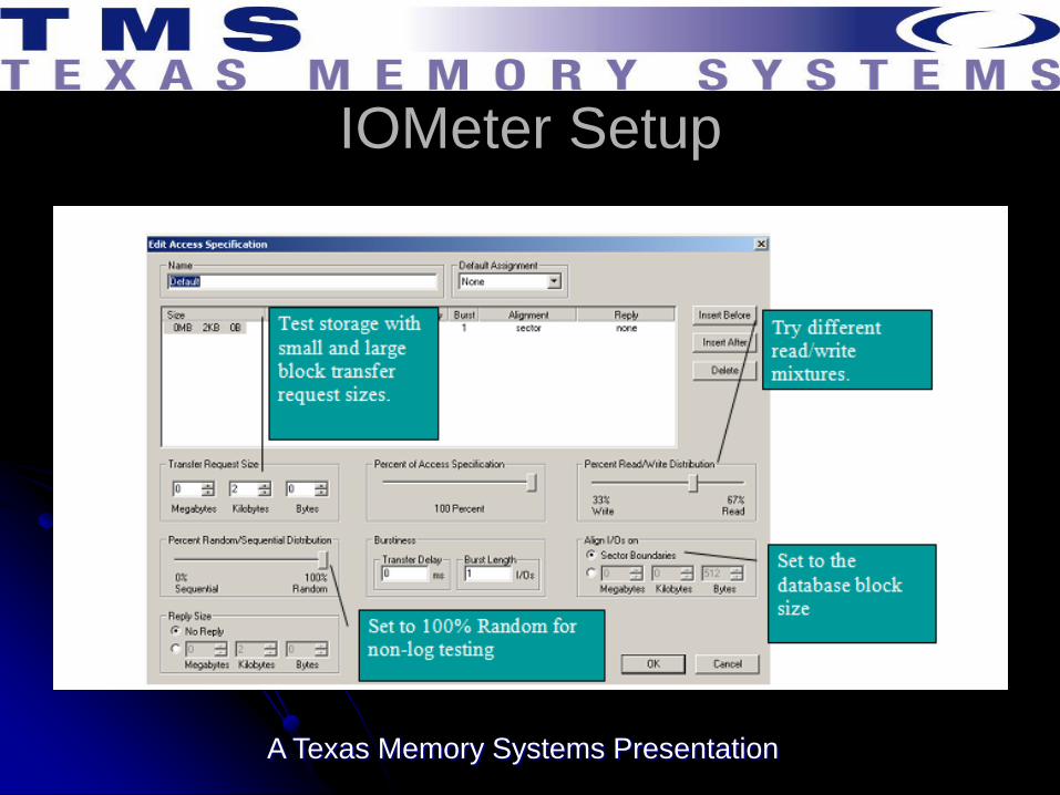
Simulating a storage profile

A basic simulation of a storage profile that was determined from AWR/Statspack analysis is very straightforward with IOmeter. Simply set a single worker to test a target storage device and put the measured storage profile metrics in the following configuration locations: Measured Application Queue = # of oustanding I/Os.

Average Request Size = Transfer Request size.

Set the measured read/write distribution.

Set the test to 100% random.

Align I/Os by the Std Block Size.


Example Runs 8 KB blocksize, 100% read access, with a queue depth of 4.

RamSan 300 (Write Accelerator) results


Examples

Little’s Law relates response time, queue

depth, and IOPS. Here IOPS (40755) *

response time (0.0000975 seconds) = 4 as

expected.


Example Runs 8 KB blocksize, 100% read access, with a queue depth of 4.

90 drive disk array


Examples

Notice that Little’s Law is still maintained:

IOPS (790) * response time (0.00506

seconds) = 4, the workload’s queue depth.


Oracle's ORION

ORION (ORacle I/O Numbers) is a tool designed by Oracle to predict the performance of an Oracle database without having to install Oracle or create a database.

It simulates Oracle I/O by using the same software stack and simulates the effect of disk striping on performance done by ASM.

It has a wide range of parameters and can be used to fully profile a storage device’s performance or run a particular I/O workload against a storage array.

ORION is available from the following URL (Requires free Oracle Technology Network login): http://www.oracle.com/technology/software/tech/orion/

http://www.oracle.com/technology/software/tech/orion/


Oracles Orion

Binaries are available for:

Linux, EM64 Linux

Solaris

Windows

AIX


Running Orion

ORION is a command line driven utility; however, a configuration file is also required.

An example ORION command would be: EX:

orion –run simple –testname <Configuation File> -num_disks 8

The configuration file contains the path to the physical drives being tested.

For example, under Windows “\\.\e:” would be the only line in the file for testing only the E: drive.

Under Linux /dev/sda specifies testing SDA.


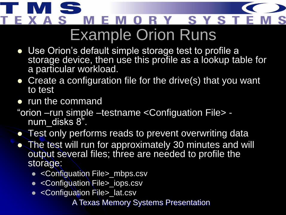
Example Orion Runs Use Orion’s default simple storage test to profile a

storage device, then use this profile as a lookup table for a particular workload.

Create a configuration file for the drive(s) that you want to test

run the command

“orion –run simple –testname <Configuation File> -num_disks 8”.

Test only performs reads to prevent overwriting data

The test will run for approximately 30 minutes and will output several files; three are needed to profile the storage: <Configuation File>_mbps.csv

<Configuation File>_iops.csv

<Configuation File>_lat.csv


Orion Simple Test These files are formatted as spreadsheets with the

columns corresponding to the number of small outstanding I/O requests and the rows corresponding to the number of large I/O requests.

The small I/O size is set to 8 KB and the large I/O is set to 1 MB.

This is meant to simulate single block reads and full table scans.

The latency and IOPS data is captured by using only small I/Os and the bandwidth is captured using only large I/Os.

The outstanding I/Os are linearly increased for both the large and small I/O case to provide a profile of the storage device’s performance.


Orion Example

Latency (8k Random Read)

0

0.2

0.4

0.6

0.8

1

1.2

0 5 10 15 20 25 30 35 40 45

Outstanding IOs

Late

ny (

ms)

IOPS (8k Random Read)

0

5000

10000

15000

20000

25000

30000

35000

40000

45000

0 5 10 15 20 25 30 35 40 45

Outstanding IOs

IOP

S

An example of the latency and IOPS output from the simple

test on the RamSan-300


Orion Examples The output data can be used with the application storage

profile to compare different storage devices’ behavior.

First run a “long” version of the test to get the performance of mixed small and large I/Os for a full storage profile.

Next, take the measured average request size to determine the right ratio of small and large I/O requests.

The measured queue depth is the sum of the large and small I/O requests, and combined with the small/large ratio will identify which data point in the output files from ORION is closest to the measured storage profile.

The profiles of different storage devices can be compared at this point to determine if they would be better for this workload.


Oracle11g Calibrate IO

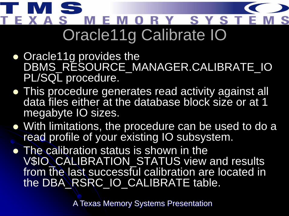
Oracle11g provides the DBMS_RESOURCE_MANAGER.CALIBRATE_IO PL/SQL procedure.

This procedure generates read activity against all data files either at the database block size or at 1 megabyte IO sizes.

With limitations, the procedure can be used to do a read profile of your existing IO subsystem.

The calibration status is shown in the V$IO_CALIBRATION_STATUS view and results from the last successful calibration are located in the DBA_RSRC_IO_CALIBRATE table.


Running Calibrate IO To perform a calibration using CALIBRATE_IO you must

have the SYSDBA privilege and the database must use async IO: filsystemio_options set to ASYNC or SETALL

timed_statistics set to TRUE.

Only one calibration run is allowed at a time. In a RAC environment the IO is spread across all nodes.

Provide the maximum number of disks and the maximum acceptable latency (between 10-100 milliseconds) and the CALIBRATE_IO package returns: Maximum sustained IOs per second (IOPS) (db block size random

reads),

Throughput in megabytes per second (1 megabyte random reads) and

Maximum throughput for any one process in process megabytes per second.


Calibrate IO Variables


Using CALIBRATE_IO

The HDD tests here were run using a dual node RAC cluster with a NexStor18F-18 disk array and a NexStor8F-8 disk array for storage, 2 of the disks were used for OCFS leaving 24 disks for use in ASM with normal redundancy.

The disk arrays utilized a 1GB Fibre Channel switch via dual paths and RedHat 4 mpio software.

The system ran on Oracle11g with the 11.1.0.7 release of the software.


Finger Printing Your IO Subsystem

The first test is for various numbers of disks (1 to

n, I used 1-30 for the 24 disk subsystem) and a

fixed allowable latency (for disks: 30 ms).

Use a PL/SQL procedure that runs the

CALIBRATE_IO routine and stores the results in

a permanent table called CAL_IO, which is

created using a CTAS from the

DBA_RSRC_IO_CALIBRATE table.


PL/SQL Script

set serveroutput on

Declare

v_max_iops PLS_INTEGER:=1;

v_max_mbps PLS_INTEGER:=1;

v_actual_latency PLS_INTEGER:=1;

i integer;

begin

for i in 1..30 loop

dbms_resource_manager.calibrate_io(i,30,

max_iops=>v_max_iops,

max_mbps=>v_max_mbps,

actual_latency=>v_actual_latency);

dbms_output.put_line('Results follow: ');

dbms_output.put_line('Max IOPS: '||v_max_iops);

dbms_output.put_line('Max MBPS: '||v_max_mbps);

dbms_output.put_line('Actual Latency: '||v_actual_latency);

insert into io_cal select * from dba_rsrc_io_calibrate;

commit;

end loop;

end;

/


Calibrate IO Results IOPS verses Disks

0

100

200

300

400

500

600

700

800

900

1000

1 3 5 7 9 11 13 15 17 19 21 23 25 27 29

Disks

Iop

s

Laency

Max IOPS

Max MBPS

Max PMBPS


Keeping Disk Count Constant

and Increasing Latency - HDD

In the second test, hold the number of

disks constant at what level you deem

best (I chose 6) and vary the acceptable

latency.


PL/SQL Routine set serveroutput on

Declare

v_max_iops PLS_INTEGER:=1;

v_max_mbps PLS_INTEGER:=1;

v_actual_latency PLS_INTEGER:=1;

i integer;

begin

for i in 10..100 loop

if (mod(i,5):=0) then

dbms_resource_manager.calibrate_io(I,30,

max_iops=>v_max_iops, max_mbps=>v_max_mbps,

actual_latency=>v_actual_latency);

dbms_output.put_line(‘Results follow: ‘);

dbms_output.put_line(‘Max IOPS: ‘||v_max_iops);

dbms_output.put_line(‘Max MBPS: ‘||v_max_mbps);

dbms_output.put_line(‘Actual Latency: ‘||v_actual_latency);

insert into io_cal select * from dba_rsrc_io_calibrate;

commit;

end if;

end loop;

end;


Results IOPS per Latency 6 Disks

0

100

200

300

400

500

600

700

800

900

1000

1100

1200

1300

1400

1500

1600

11 15 18 23 28 35 40 46 49 54 59 65 71 75 78 87 92 93 102

Latency

IOP

S

Max IopsMax MBPSMax PMBPS


HDD Results This is an unexpected result based on a derivation of Little’s law

(IOPS=QUEUE/Response time) which seems to indicate that as the response time (latency) is allowed to increase with a fixed queue size (6 disks) the IOPS should decrease.

It can only be assumed that the number of disks is not being used as a queue size determiner in the procedure.

What this does show is that if we allow latency to creep up, as long as we don’t exceed the queue capability of the IO subsystem, we will get increasing IOPS.

The maximum throughput hovers around 100, but unlike in the first test there is no overall downward trend, seeming to indicate as the number of disks input into the procedure increases, the overall throughput trends slightly downward.

The process maximum throughput hovered around 30, just like in the previous test.


HDD Results

During my tests the average queue according to iostat was at 16 with jumps to 32 on some disks but not all.

The utilization for each disk was at about 40-50 with peaks as high as 90 depending on the test. I suggest monitoring queue depth with OS monitoring tools during the test.

Based on the two result sets you should be able to determine the best final run settings to load the DBA_RSRC_IO_CALIBRATE table with to get your best results.


SDD and Calibrate IO

Latency starts at 10 milliseconds. That makes it useless for profiling SSD based components because even the worst- performing SSDs achieve max latencies of less than 2 milliseconds with most being less than 1 millisecond.

Developer of this package obviously had never heard of SSDs, has never profiled SSDs and wasn’t addressing this for use with SSDs.

The package should be re-written to allow starting at 100 microseconds and ramping up at 100 microsecond intervals to 2000 microseconds to be useful for SSD profiling and testing.


SSD Results – Increasing Latency

SSD IOPS Per Latency 6 Disks

1

10

100

1000

10000

100000

1000000

10 15 20 25 30 35 40 45 50 55

Set Latency

IOP

S

Latency

Max Iops

Max MBPS

Max PMBPS


SSDs and Calibrate IO

At the lowest allowed latency, 10ms, the IOPS for the SSD are maxed out

The procedure does no write testing, only read testing.

I agree that with the lazy write algorithms (delayed block cleanout for you old timers) that writes aren’t generally important in the context of Oracle performance, except when those writes interfere with reads, which for disk systems is generally always.

So, while the CALIBRATE_IO procedure has limited usability for disk based systems (most of whom have less than 10 ms latency) it will have less and less usefulness as SSDs push their way into the data center.


Summary

Understanding storage’s behavior can be a very powerful tool.

The mathematical relationships can seem a bit unwieldy but are actually quite simple and easy to master.

Oracle provides very comprehensive data in AWR or Statspack reports that include a wealth of data about what load the application is creating on the storage device and how the storage is handling it.

Using this data, various storage devices can quickly be tested in a simple benchmark environment that accurately simulates a large production workload.

validating you io subsystem - new york oracle user...

Documents