uwe mühlich fundamentals of tensor calculus for engineers
TRANSCRIPT

Solid Mechanics and Its Applications
Uwe Mühlich
Fundamentals of Tensor Calculus for Engineers with a Primer on Smooth Manifolds
Solid Mechanics and Its Applications
Volume 230
Series editors
J.R. Barber, Ann Arbor, USAAnders Klarbring, Linköping, Sweden
Founding editor
G.M.L. Gladwell, Waterloo, ON, Canada

Aims and Scope of the Series
The fundamental questions arising in mechanics are: Why?, How?, and How much?The aim of this series is to provide lucid accounts written by authoritativeresearchers giving vision and insight in answering these questions on the subject ofmechanics as it relates to solids.
The scope of the series covers the entire spectrum of solid mechanics. Thus itincludes the foundation of mechanics; variational formulations; computationalmechanics; statics, kinematics and dynamics of rigid and elastic bodies: vibrationsof solids and structures; dynamical systems and chaos; the theories of elasticity,plasticity and viscoelasticity; composite materials; rods, beams, shells andmembranes; structural control and stability; soils, rocks and geomechanics;fracture; tribology; experimental mechanics; biomechanics and machine design.
The median level of presentation is to the first year graduate student. Some textsare monographs defining the current state of the field; others are accessible to finalyear undergraduates; but essentially the emphasis is on readability and clarity.
More information about this series at http://www.springer.com/series/6557

Uwe Mühlich
Fundamentals of TensorCalculus for Engineerswith a Primer on SmoothManifolds
123
Uwe MühlichFaculty of Applied EngineeringUniversity of AntwerpAntwerpBelgium
ISSN 0925-0042 ISSN 2214-7764 (electronic)Solid Mechanics and Its ApplicationsISBN 978-3-319-56263-6 ISBN 978-3-319-56264-3 (eBook)DOI 10.1007/978-3-319-56264-3
Library of Congress Control Number: 2017935015
© Springer International Publishing AG 2017This work is subject to copyright. All rights are reserved by the Publisher, whether the whole or partof the material is concerned, specifically the rights of translation, reprinting, reuse of illustrations,recitation, broadcasting, reproduction on microfilms or in any other physical way, and transmissionor information storage and retrieval, electronic adaptation, computer software, or by similar or dissimilarmethodology now known or hereafter developed.The use of general descriptive names, registered names, trademarks, service marks, etc. in thispublication does not imply, even in the absence of a specific statement, that such names are exempt fromthe relevant protective laws and regulations and therefore free for general use.The publisher, the authors and the editors are safe to assume that the advice and information in thisbook are believed to be true and accurate at the date of publication. Neither the publisher nor theauthors or the editors give a warranty, express or implied, with respect to the material contained herein orfor any errors or omissions that may have been made. The publisher remains neutral with regard tojurisdictional claims in published maps and institutional affiliations.
Printed on acid-free paper
This Springer imprint is published by Springer NatureThe registered company is Springer International Publishing AGThe registered company address is: Gewerbestrasse 11, 6330 Cham, Switzerland

Preface
Continuum mechanics and its respective subtopics such as strength of materials,theory of elasticity, and plasticity are of utmost importance for mechanical and civilengineers. Tensors of different types, such as vectors and forms, appear mostnaturally in this context. Ultimately, when it comes to large inelastic deformations,operations like push-forward, pull-back, covariant derivative, and Lie derivativebecome inevitable. The latter form a part of modern differential geometry, alsoknown as tensor calculus on differentiable manifolds.
Unfortunately, in many academic institutions, an engineering education stillrelies on conventional vector calculus and concepts like dual vector space, andexterior algebra are successfully ignored. The expression “manifold” arises more orless as a fancy but rather diffuse technical term. Analysis on manifolds is onlymastered and applied by a very limited number of engineers. However, the mani-fold concept has been established now for decades, not only in physics but, at leastin parts, also in certain disciplines of structural mechanics like theory of shells.Over the years, this has caused a large gap between the knowledge provided toengineering students and the knowledge required to master the challenges, con-tinuum mechanics faces today.
The objective of this book is to decrease this gap. But, as the title alreadyindicates, it does not aim to give a comprehensive introduction to smooth mani-folds. On the contrary, at most it opens the door by presenting fundamentalconcepts of analysis in Euclidean space in a way which makes the transition tosmooth manifolds as natural as possible.
The book is based on the lecture notes of an elective course on tensor calculustaught at TU-Bergakademie Freiberg. The audience consisted of master students inMechanical Engineering and Computational Materials Science, as well as doctoralstudents of the Faculty of Mechanical, Process and Energy Engineering. Thisintroductory text has a special focus on those aspects of which a thorough under-standing is crucial for applying tensor calculus safely in Euclidean space, partic-ularly for understanding the very essence of the manifold concept. Mathematicalproofs are omitted not only because they are beyond the scope of the book butalso because the author is an engineer and not a mathematician. Only in some
v
particular cases are proofs sketched in order to raise awareness of the effort made bymathematicians to work out the tools we are using today. In most cases, however,the interested reader is referred to corresponding literature. Furthermore, invariants,isotropic tensor functions, etc., are not discussed, since these subjects can be foundin many standard textbooks on continuum mechanics or tensor calculus.
Prior knowledge in real analysis, i.e., analysis in R, is assumed. Furthermore,students should have a prior education in undergraduate engineering mechanics,including statics and strength of materials. The latter is surely helpful for under-standing the differences between the traditional and modern version of tensorcalculus.
Antwerp, Belgium Uwe MühlichFebruary 2017
vi Preface
Acknowledgements
I would like to express my gratitude to my former colleagues of the solid mechanicsgroup of the Institute of Mechanics and Fluid Dynamics at TU-BergakademieFreiberg, and in particular to Michael Budnitzki, Thomas Linse, and ChristophHäusler. Without their open-minded interest in the subject and their constantreadiness to discuss it, this book would not exist. I am especially grateful to HeinzGründemann for his support and inspiring discussions about specific topics relatedto the subject. In this context, I would also like to thank Jarno Hein, who brought usinto contact.
Additionally, this book could not have been accomplished without the educationI received in engineering mechanics, and I would like to take this opportunity toexpress my sincere gratitude to my teachers, Reinhold Kienzler and WolfgangBrocks.
I would like to thank TU-Bergakademie Freiberg and especially Meinhard Kunafor the opportunity to teach a course about tensor calculus and for providing thefreedom to teach a continuum mechanics lecture during the summer term of 2014which deviated significantly from the approach commonly applied in engineeringeducation. In addition, I would like to express my appreciation to all students andcolleagues who attended the courses mentioned above for their interest and aca-demic curiosity, but especially for critical remarks which helped to uncover mis-takes and to clarify doubts.
Besides, I would like to acknowledge the support provided by the Faculty ofApplied Engineering of the University of Antwerp in terms of infrastructure andtime necessary to finalize the process of converting the course notes into a book.
Furthermore, I would like to thank Nathalie Jacobs, Almitra Gosh, Naga KumarNatti, Henry Pravin, and Cynthia Feenstra from Springer Scientific Publishing fortheir support throughout the process of publishing this book. My thanks are alsodue to Marc Beschler for language editing the book.
vii

Contents
1 Introduction . . . . . . . . . . . . . . . . . . . . . . . . . . . . . . . . . . . . . . . . . . . . . . 11.1 Space, Geometry, and Linear Algebra . . . . . . . . . . . . . . . . . . . . . 11.2 Vectors as Geometrical Objects . . . . . . . . . . . . . . . . . . . . . . . . . . 21.3 Differentiable Manifolds: First Contact . . . . . . . . . . . . . . . . . . . . . 31.4 Digression on Notation and Mappings . . . . . . . . . . . . . . . . . . . . . 6References. . . . . . . . . . . . . . . . . . . . . . . . . . . . . . . . . . . . . . . . . . . . . . . . 8
2 Notes on Point Set Topology. . . . . . . . . . . . . . . . . . . . . . . . . . . . . . . . . 92.1 Preliminary Remarks and Basic Concepts. . . . . . . . . . . . . . . . . . . 92.2 Topology in Metric Spaces . . . . . . . . . . . . . . . . . . . . . . . . . . . . . . 102.3 Topological Space: Definition and Basic Notions . . . . . . . . . . . . . 152.4 Connectedness, Compactness, and Separability. . . . . . . . . . . . . . . 172.5 Product Spaces and Product Topologies . . . . . . . . . . . . . . . . . . . . 192.6 Further Reading . . . . . . . . . . . . . . . . . . . . . . . . . . . . . . . . . . . . . . 21References. . . . . . . . . . . . . . . . . . . . . . . . . . . . . . . . . . . . . . . . . . . . . . . . 22
3 The Finite-Dimensional Real Vector Space . . . . . . . . . . . . . . . . . . . . . 233.1 Definitions . . . . . . . . . . . . . . . . . . . . . . . . . . . . . . . . . . . . . . . . . . 233.2 Linear Independence and Basis. . . . . . . . . . . . . . . . . . . . . . . . . . . 253.3 Some Common Examples for Vector Spaces . . . . . . . . . . . . . . . . 283.4 Change of Basis . . . . . . . . . . . . . . . . . . . . . . . . . . . . . . . . . . . . . . 293.5 Linear Mappings Between Vector Spaces . . . . . . . . . . . . . . . . . . . 303.6 Linear Forms and the Dual Vector Space . . . . . . . . . . . . . . . . . . . 323.7 The Inner Product, Norm, and Metric. . . . . . . . . . . . . . . . . . . . . . 353.8 The Reciprocal Basis and Its Relations with the Dual Basis. . . . . 37References. . . . . . . . . . . . . . . . . . . . . . . . . . . . . . . . . . . . . . . . . . . . . . . . 40
4 Tensor Algebra . . . . . . . . . . . . . . . . . . . . . . . . . . . . . . . . . . . . . . . . . . . 414.1 Tensors and Multi-linear Forms . . . . . . . . . . . . . . . . . . . . . . . . . . 414.2 Dyadic Product and Tensor Product Spaces . . . . . . . . . . . . . . . . . 434.3 The Dual of a Linear Mapping . . . . . . . . . . . . . . . . . . . . . . . . . . . 46
ix

4.4 Remarks on Notation and Inner Product Operations . . . . . . . . . . . 464.5 The Exterior Product and Alternating Multi-linear Forms. . . . . . . 484.6 Symmetric and Skew-Symmetric Tensors . . . . . . . . . . . . . . . . . . . 504.7 Generalized Kronecker Symbol . . . . . . . . . . . . . . . . . . . . . . . . . . 514.8 The Spaces KkV and KkV� . . . . . . . . . . . . . . . . . . . . . . . . . . . . . . 524.9 Properties of the Exterior Product and the Star-Operator . . . . . . . 534.10 Relation with Classical Linear Algebra. . . . . . . . . . . . . . . . . . . . . 55References. . . . . . . . . . . . . . . . . . . . . . . . . . . . . . . . . . . . . . . . . . . . . . . . 57
5 Affine Space and Euclidean Space . . . . . . . . . . . . . . . . . . . . . . . . . . . . 595.1 Definitions and Basic Notions . . . . . . . . . . . . . . . . . . . . . . . . . . . 595.2 Alternative Definition of an Affine Space
by Hybrid Addition . . . . . . . . . . . . . . . . . . . . . . . . . . . . . . . . . . . 615.3 Affine Mappings, Coordinate Charts
and Topological Aspects. . . . . . . . . . . . . . . . . . . . . . . . . . . . . . . . 62References. . . . . . . . . . . . . . . . . . . . . . . . . . . . . . . . . . . . . . . . . . . . . . . . 67
6 Tensor Analysis in Euclidean Space. . . . . . . . . . . . . . . . . . . . . . . . . . . 696.1 Differentiability in R and Related Concepts Briefly Revised . . . . 696.2 Generalization of the Concept of Differentiability. . . . . . . . . . . . . 726.3 Gradient of a Scalar Field and Related Concepts in RN . . . . . . . . 736.4 Differentiability in Euclidean Space Supposing
Affine Relations . . . . . . . . . . . . . . . . . . . . . . . . . . . . . . . . . . . . . . 776.5 Characteristic Features of Nonlinear Chart Relations . . . . . . . . . . 846.6 Partial Derivatives as Vectors and Tangent Space at a Point . . . . 866.7 Curvilinear Coordinates and Covariant Derivative . . . . . . . . . . . . 896.8 Differential Forms in RN and Integration . . . . . . . . . . . . . . . . . . . 936.9 Exterior Derivative and Stokes’ Theorem in Form Language . . . . 95References. . . . . . . . . . . . . . . . . . . . . . . . . . . . . . . . . . . . . . . . . . . . . . . . 98
7 A Primer on Smooth Manifolds . . . . . . . . . . . . . . . . . . . . . . . . . . . . . . 997.1 Introduction . . . . . . . . . . . . . . . . . . . . . . . . . . . . . . . . . . . . . . . . . 997.2 Basic Concepts Regarding Analysis on Surfaces in R3. . . . . . . . . 1037.3 Transition to Smooth Manifolds . . . . . . . . . . . . . . . . . . . . . . . . . . 1087.4 Tangent Bundle and Vector Fields . . . . . . . . . . . . . . . . . . . . . . . . 1097.5 Flow of Vector Fields and the Lie Derivative. . . . . . . . . . . . . . . . 1147.6 Outlook and Further Reading . . . . . . . . . . . . . . . . . . . . . . . . . . . . 118References. . . . . . . . . . . . . . . . . . . . . . . . . . . . . . . . . . . . . . . . . . . . . . . . 119
Solutions for Selected Problems . . . . . . . . . . . . . . . . . . . . . . . . . . . . . . . . . 121
Index . . . . . . . . . . . . . . . . . . . . . . . . . . . . . . . . . . . . . . . . . . . . . . . . . . . . . . 123
x Contents
Selected Symbols
N Set of natural numbersZ Set of integer numbersQ Set of rational numbersR Set of real numbersC Set of complex numbers\ Intersection of sets: A\B ¼ fxjx 2 A and x 2 Bg[ Union of sets: A[B ¼ fxjx 2 A or x 2 Bg� Subset A � BAc Complement of a set AA ! B Mapping from set A to set Bu;ex Vector, dual vector
⊕, ⊞, + Symbols used to indicate addition of elements of a vector space⊙, ⊡ Symbols used to indicate multiplication of elements of a vector space by
a real numberHybrid addition between points and vectors
^ Exterior product�u Star operator applied to a vectorgH; gH Push forward and pull back operation under a mapping g> General tensordki Kronecker symbol, see (3.9)
edjpf ðuÞ Directional derivative of the function f at point p in direction u
›ijp Tangent vector at a point p on a smooth manifold
e›ijp Cotangent vector at a point p on a smooth manifold
xi

@@xi��lðpÞ Tangent vector at the image of point p in a chart generated by a mapping
l with coordinates xi
edjlðpÞxi Cotangent vector at the image of point p in a chart generated by a
mapping l with coordinates xi
xii Selected Symbols
Chapter 1Introduction
Abstract The introduction aims to remind the reader that engineering mechanics isderived from classical mechanics, which is a discipline of general physics. Therefore,engineering mechanics also relies on a proper model for space, and the relationsbetween space andgeometry are discussed briefly. The idea of expressing geometricalconcepts by means of linear algebra is sketched together with the concept of vectorsas geometrical objects. Although this book provides only the very first steps of themanifold concept, this chapter intends to make its importance for modern continuummechanics clear by raising a number of questions which cannot be answered by theconventional approach. Furthermore, aspects regarding mathematical notation usedin subsequent chapters are discussed briefly.
1.1 Space, Geometry, and Linear Algebra
One of the most important tools for mechanical and civil engineers is certainlymechanics, and in particular continuum mechanics, together with its subtopics, lin-ear and nonlinear elasticity, plasticity, etc. Mechanics is about the motion of bodiesin space. Therefore, a theory of mechanics first requires concepts of space and time,particularly space–time, and, in addition, a concept to make the notion of a materialbody more precise. Traditionally, the scientific discipline concerned with the formu-lation of models for space is geometry. Starting from a continuum perspective ofspace–time, the simplest model one can think of is obtained by assuming euclideangeometry for space and by treating time separately as a simple scalar parameter.
In two-dimensional euclidean geometry, points and straight lines are primitiveobjects and the theory of euclidean space is based on a series of axioms. The mostcrucial one is the fifth postulate, which distinguishes euclidean geometry from otherpossible geometries. It introduces a particular notion of parallelism, and one way toexpress this in two dimensions is as follows. Given a straight line L , there is onlyone straight line through a point P not on L which never meets L .
It took mankind centuries to understand that euclidean geometry is only one ofmany possible geometries, see e.g., Holme [2] and BBC [1]. But, once this funda-mental fact had been discovered, it became apparent rather quickly that the question
© Springer International Publishing AG 2017U. Mühlich, Fundamentals of Tensor Calculus for Engineers with a Primeron Smooth Manifolds, Solid Mechanics and Its Applications 230,DOI 10.1007/978-3-319-56264-3_1
1

2 1 Introduction
as to which space or space–time model is appropriate for developing a particulartheory of physics can only be answered through experiments and not just throughlogical reasoning.
Historically, mechanics has been developed based on the assumption that euclid-ean space is an appropriate model for our physical space, i.e., the space we live inperforming observations and measurements. The idea of force as an abstract conceptof what causes a change in the motion of a body was a cornerstone of this devel-opment. However, at the beginning of the twentieth century, it became apparent totheoretical physicists that physical space is actually curved, and gravitation is seennowadays as the cause for space curvature. Models for space, other than euclideangeometry, had to be employed in order to develop the corresponding theories.
In the course of this development, it became clear as well that new mathematicaltools are required in order to encode new physical ideas properly. Tensor analy-sis using Ricci calculus was elaborated, Grassmann algebra was rediscovered, thedifferentiable manifold concept gained more and more use in theoretical physics,etc. Nowadays, these tools are matured and rather well established. However, theprocess of using them for reformulating existing theories in order to gain deeperunderstanding, is still going on.
Differentiablemanifolds are by definition objects which are at least locally euclid-ean. Therefore, affine and euclidean geometry are crucial for the treatment of moregeneral differentiablemanifolds. Although linear algebra is not the same as euclideangeometry, the former provides concepts which can be used to formulate euclideangeometry in an elegant way by employing the vector space concept. A straight linein the language of linear algebra is a point combined with a the scalar multiple ofa vector. Euclidean parallelism is expressed by the notion of linear dependence ofvectors, etc.
1.2 Vectors as Geometrical Objects
Most of us were confronted with vectors for the first time in the following way.Starting with the definition that a vector a is an object which possesses directionand magnitude, this object is visualized by taking, e.g., a sheet of paper, drawing astraight line of some length, related to the magnitude, and indicating the directionby an arrow. Afterwards, it is agreed upon that two vectors are equal if they havesame length and direction. A further step consists in the definition of two operations,namely the addition of vectors and multiplication of a vector with a real number. Atthis stage, these operations are defined only graphically, which can be expressed bythe following definitions.
Definition 1.1 (Addition of two vectors (graphically)) In order to determine thesum c of two vectors a and b graphically, written as c = a ⊕ b
1. displace a and b in parallel such that the head of a meets the tail of b and2. c is the directed line from the tail of a to the head of b,
1.2 Vectors as Geometrical Objects 3
where displace in parallel means to move the corresponding vector without changingits length or direction.
Definition 1.2 (Multiplication of a vector with a real number (graphically)) Themultiplication of a vector a of length ||a|| with a real number α gives a vector d withlength |α| ||a||. If α > 0, then the directions of a and d coincide, and if α < 0 thend has the direction opposite to that of a.
Of course, it is rather tedious to perform this operations graphically. This alreadygives motivation for an algebraic definition, which allows for a computation withnumbers instead of performing graphical operations by means of drawings andeventually extracting the results with rulers. This algebraic definition, which willbe discussed with more rigor later on, is based on the idea of defining vectors bytheir behavior under the operations mentioned above, leading to the notion of thevector space.
However, there is more which motivates an algebraic treatment of vectors. Avery common picture from structural mechanics is the following. Some structure,for example, a straight beam, is drawn on a sheet of paper together with two forcevectors acting on it. The position of the beam in space, for which the paper is a kindof image or model, is indicated by position vectors after choosing an origin. Theresulting force is now obtained by the method defined by Definition1.1. Although,this picture is seemingly quite intuitive, and is widely used also by the author, thereare some serious objections against it. The most important one is, that the space ofobservationS, and vector spaceswith different underlyingmeanings are freelymixedtogether. This may, and often does, cause severe confusions when approaching morecomplex problems.
1.3 Differentiable Manifolds: First Contact
A general idea about space is that it consists of points together with a topology. Onlyin the presence of the latter does it make sense to talk about neighborhoods, interiorand boundary of objects, etc. For a large number of problems, a three dimensionaleuclidean space is an appropriate model for physical space. Objects and operationsbetween themcan be defined in accordancewith the properties of euclidean space, butthose operations can only be performed symbolically. In order to allow for computa-tion with numbers, the points of this space are labeled by triples of real numbers afterchoosing an origin which gets the label (0, 0, 0). These labels are called coordinates.Through such a labeling, we actually generate a chart of our space of observationand all computations are performedwithin this chart. For a three-dimensional euclid-ean space, a single chart is sufficient which coincides with the R3. Technically, wemap points from one euclidean space into a particular representative of an euclideanspace in which computations can be carried out. In order to quantify observationsin space, like the motion of some body, these observations are first transferred, andhence mapped, into the chart.
4 1 Introduction
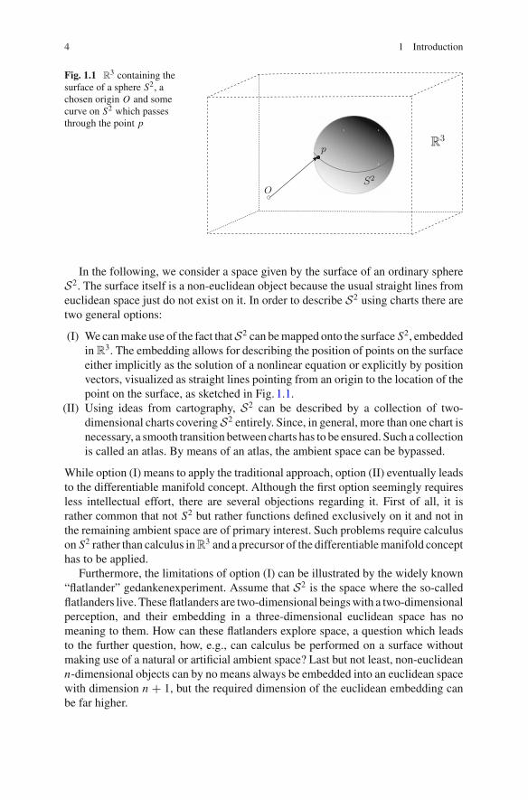
Fig. 1.1 R3 containing the
surface of a sphere S2, achosen origin O and somecurve on S2 which passesthrough the point p
S2
R3
O
p
In the following, we consider a space given by the surface of an ordinary sphereS2. The surface itself is a non-euclidean object because the usual straight lines fromeuclidean space just do not exist on it. In order to describe S2 using charts there aretwo general options:
(I) We canmake use of the fact thatS2 can bemapped onto the surface S2, embeddedinR3. The embedding allows for describing the position of points on the surfaceeither implicitly as the solution of a nonlinear equation or explicitly by positionvectors, visualized as straight lines pointing from an origin to the location of thepoint on the surface, as sketched in Fig. 1.1.
(II) Using ideas from cartography, S2 can be described by a collection of two-dimensional charts covering S2 entirely. Since, in general, more than one chart isnecessary, a smooth transition between charts has to be ensured. Such a collectionis called an atlas. By means of an atlas, the ambient space can be bypassed.
While option (I) means to apply the traditional approach, option (II) eventually leadsto the differentiable manifold concept. Although the first option seemingly requiresless intellectual effort, there are several objections regarding it. First of all, it israther common that not S2 but rather functions defined exclusively on it and not inthe remaining ambient space are of primary interest. Such problems require calculuson S2 rather than calculus inR3 and a precursor of the differentiablemanifold concepthas to be applied.
Furthermore, the limitations of option (I) can be illustrated by the widely known“flatlander” gedankenexperiment. Assume that S2 is the space where the so-calledflatlanders live. These flatlanders are two-dimensional beingswith a two-dimensionalperception, and their embedding in a three-dimensional euclidean space has nomeaning to them. How can these flatlanders explore space, a question which leadsto the further question, how, e.g., can calculus be performed on a surface withoutmaking use of a natural or artificial ambient space? Last but not least, non-euclideann-dimensional objects can by no means always be embedded into an euclidean spacewith dimension n + 1, but the required dimension of the euclidean embedding canbe far higher.

1.3 Differentiable Manifolds: First Contact 5
Nevertheless, there are usually objections with regard to the second option too.The most common of these is:
For the problems I am working on, the concept of euclidean space is sufficient.
However, just by drawing the sketch and thinking about it before the additionof any technical details, important questions arise from the argument that physicalphenomena are just there and do not depend on our way of describing them, e.g., byusing a natural or artificial embedding. Some of these questions are:
• Global vector balances, like the global balance of momentum in continuummechanics, rely on the parallel transport of vectors in euclidean space. There-fore, those balances only have a meaning in euclidean space. Can such statementsactually be general laws of physics at all?
• Another concept widely used in continuummechanics is the concept of invarianceunder finite rigid body motion. Imagine continuum mechanics on a surface withchanging curvature. A finite rigid body motion is just not possible in this case.
• If something is moving in a non-euclidean space, there is still a velocity for whichit makes sense to talk about a direction and amagnitude. Hence, the vector conceptwill be needed in non-euclidean spaces as well. But how to work with vectors inthis case without any embedding?
At the end of this short introduction, another argument employed frequently toavoid the manifold concept should be mentioned. It goes as follows:
Even if the manifold approach could give me more insight, it seems far too complicated, andtraditional vector calculus works fine for me.
It is true that the mere act of obtaining even a basic understanding of the calculus ondifferentiable manifolds requires considerable effort. However, some tedious mat-ters, for example integration theorems, becomemuch easier. Furthermore, traditionalvector calculus also relies on an underlying manifold approach. One just does not seeit because it remains hidden all the time. A main objective of this book is to uncoverthis underlying approach.
Last but not least, most engineers design and develop constructions, machinery,and devices in order to get things done. Smart engineering solutions usually alsopossess certain aesthetics easily discerned by other engineers. In the end, linearalgebra, analysis, etc., as well as calculus on manifolds are mental constructionsdesigned to get things done safely and as efficiently as possible. And most likely,greater familiarity with these constructions will cause their efficiency and eleganceto become apparent.

6 1 Introduction
1.4 Digression on Notation and Mappings
Engineers and physicists are not the only ones to express concepts and ideas inwords before translating them into the language ofmathematics. Regarding the latter,some standards have evolved over time which are subsumed here under the termmathematical notation. The use of such a notation does not make ideas or conceptssmarter and it does not change the principal informational content either. However,a standardized notation is not only more concise and encourages precision, but theinformation can also be accessed by a larger group of people and not just by alimited community. Furthermore, notation helps in discovering structural similaritiesbetween concepts which might have emerged in different contexts.
Although it is assumed that the reader does possess knowledge of applied mathe-matics at least at the undergraduate level, a few explanatory remarks seemappropriateat this point. The concept of a function is undoubtedly one of the most widely usedin all areas of engineering and science. The notation commonly used in school or inundergraduate courses in applied mathematics at universities, for instance,
f (n) = √n , n ∈ N , (1.1)
is sufficient to understand that the function f takes a natural number as argumentand that it delivers a real number. Therefore, f relates every element of the set ofnatural numbers N to an element of the set of real numbers R. In other words, f isa mapping of N into R. This concept also applies to sets, the elements of which canbe objects of any kind.
Definition 1.3 (Mapping) Given two sets D and C . A mapping M from D to C ,written as M : D → C , relates every element of D to at least one element of C . Dis called domain whereas C is referred to as co-domain.
The notation
f : N → R , (1.2)
emphasizes that f is only a particular case of amapping. If more specific informationabout f is available, e.g., (1.1), then (1.2) is supplemented by it, i.e.,
n �→ a = √n
which leads to the use of the combined notation
f : N → R
n �→ a = √n
instead of (1.1).
1.4 Digression on Notation and Mappings 7
Definition 1.4 (Cartesian product) The Cartesian product between two sets A andB, written as A×B, is a set which contains all ordered pairs (a, b)with a ∈ A, b ∈ B.
For instance, a mapping
f : N × N → R
(m, n) �→ a = √m + n
takes two natural numbers and delivers a real number.Furthermore, some essential properties of generalmappingswill be briefly revised
next. These properties will become rather important in the next chapters.
Definition 1.5 (Injective mapping) A mapping D → C is called injective or one-to-one if every element of D is mapped to exactly one element of C .
Definition 1.6 (Surjective mapping) Amapping D → C is called surjective or ontoif at least one element of D corresponds to every element of C .
Definition 1.7 (Bijective mapping) A mapping is called bijective if it is injectiveand surjective.
Often, it is not only one mapping but rather the composition of various mappingsthat is of interest. Consider the mappings
f : R → R × R (1.3)
t �→ (cos t, 2 sin t)
and
g : R × R → R (1.4)
(x, y) �→ √x2 + y2
as an example. The composition h = g ◦ f is a mapping
h : R → R (1.5)
τ �→√cos2 τ + sin2 τ ,
and so-called commutative diagrams, as shown in Fig. 1.2, are commonly used tovisualize such situations. The interested reader is referred to Valenza [3].
Before getting into the main matter, some general aspects of notation issuesshould be discussed. Ideally, notation should be as precise as possible. However, withincreasing degrees of complexity, this can lead to formulas with symbols surroundedby clouds of labels, indices, etc. Despite the comprehensiveness of the information,it usually makes it almost impossible to capture the essence of a symbol or equation,

8 1 Introduction
Fig. 1.2 Commutativediagram for the mappingsgiven by (1.3)–(1.5) R R
R × R
g ◦ f
f
g
respectively. The other extreme is to keep notation as plain as possible, leaving it tothe reader to deduce the specific meaning of symbols from the context. Here, as inmost books, a reasonable compromise is intended.
References
1. BBC (2013) Non-euclidean geometry. http://www.youtube.com/watch?v=an0dXEImGHM2. Holme A (2010) Geometry our cultural heritage, 2nd edn. Springer, Berlin3. Valenza R (1993) Linear algebra: an introduction to abstract mathematics. Undergraduate texts
in mathematics. Springer, Berlin

Chapter 2Notes on Point Set Topology
Abstract The chapter provides a brief exposition of point set topology. In particular,it aims to make readers from the engineering community feel comfortable withthe subject, especially with those topics required in latter chapters. The implicitappearanceof topological concepts in the context of continuummechanics is sketchedfirst. Afterwards, topological concepts like interior and boundary of sets, continuityof mappings, etc., are discussed within metric spaces before the introduction of theconcept of topological space.
2.1 Preliminary Remarks and Basic Concepts
Here, tensor calculus is not seen as an end in itself, but rather in the context ofengineering mechanics, particularly continuum mechanics. As already discussedearlier, the latter first requires a model for space.
Afirst step in defining such amodel is to interpret space as a set of points.However,if, for instance, different points should refer somehow to different locations, then aset of points, as such, is rather useless. Although sets already possess a kind ofstructure due to the notion of subsets and operations like union, intersection, etc.,some additional structure is required by which a concept like location makes sense.Experience tells us that location is usually expressed with respect to a previouslydefined point of reference. This, on the other hand, requires relating different pointswith each other, for instance, by means of a distance.
Distance is primarily a quantitative concept. However, apart from quantitativecharacteristics like distances between points, length of a curve, etc., there are alsoothers, commonly subsumed under the term topological characteristics. For instance,in continuum mechanics, the concept of a material body is usually introduced asfollows. A material body becomes apparent to us by occupying a region in space ata certain instant in time, i.e., a subset of the set of points mentioned above. A look atthe sketches commonly used to illustrate basic ideas of continuummechanics revealsthat it is tacitly assumed that this region is “connected” and usually has an “interior”and a “boundary.”
© Springer International Publishing AG 2017U. Mühlich, Fundamentals of Tensor Calculus for Engineers with a Primeron Smooth Manifolds, Solid Mechanics and Its Applications 230,DOI 10.1007/978-3-319-56264-3_2
9

10 2 Notes on Point Set Topology
Intuitively,we have no problemaccepting “connected,” “interior,” and “boundary”as topological properties. However, there are other properties whose topologicalcharacter is not at all that obvious. Therefore, the question arises as to how to definemore precisely what topological properties actually are. The following experimentmight give us some initial clues. A party balloon is inflated until it is possible todraw geometric figures on it. This might be called state one. Afterwards, the balloonis inflated further up to a state two. The figures can be inspected in order to workout those properties which do not change under the transition from state one to statetwo. Having this experiment in mind, one might be tempted to state that topologicalproperties are those which do not change under a continuous transformation, i.e.,a continuous mapping. However, without a precise notion of continuity, this is notreally a definition but, at best, a starting point from which eventually to work out arigorous framework. Furthermore, it turns out that not all continuous mappings aresuitable for distinguishing unambiguously topological properties from others, butrather only so-called homeomorphisms, bijective mappings which are continuous inboth directions, to be discussed in greater detail later.
The discipline which covers the problems sketched so far is called point set topol-ogy and it can be outlined in a variety of ways. Perhaps the most intuitive one is tostart with metric spaces, i.e., a set of points together with a structure which allowsus to measure distances between points. Most texts on topology in metric spacesfocus first on convergence of series and continuity. Properties of sets like interior orboundary are addressed only afterwards in order to prepare the next level of abstrac-tion, namely topological spaces. Here, however, we follow Geroch [2] and start withtopological properties of sets in metric spaces.
2.2 Topology in Metric Spaces
The concept of a metric space is a generalization of the notion of distance.Measuringdistances consists in assigning real numbers to pairs of points by means of someruler, hence, it is essentially a mapping d : X × X → R where d is called a distancefunction. A second step toward a more general scheme is to abstain from interpretingthe elements of X in a particular way. In the following, the elements of X can beobjects of any kind. By combining the set X with a distance function d, a space(X, d) is generated. Themost challenging part is to define aminimal set of rules that adistance functionmust obey such that certain concepts can be defined unambiguouslyand facts about (X, d) can be deduced by logical reasoning.
Defining this minimal set of rules is an iterative process for a variety of reasons.The design of a particular distance function has to take into account the specificnature of the elements of X . Furthermore, as in daily life, different rulers, hencedifferent distance functions, should be possible for the same X . A minimal set ofrules must cover all these cases and should therefore be rather general. In addition,the set of rules has to account for what should be agreed upon no matter whichparticular distance function is used to perform a measurement on a given set X . And

2.2 Topology in Metric Spaces 11
last but not least, for cases in which we do not even need mathematics because thingsare simply obvious just by looking at them, facts about (X, d) compiled in respectivetheorems should be in line with our intuition. The final result of this process is thefollowing definition.
Definition 2.1 (Metric) Given a point set X , a metric is a mapping
d : X × X → R
with the properties:
(i) d(p, q) > 0,(ii) d(p, q) = 0 implies p = q and vice versa,(iii) d(p, q) = d(q, p),(iv) d(p, q) ≤ d(p, r) + d(r, q),
where p, q, r ∈ X .
The most common representatives of a metric are the absolute value of the differenceof two real numbers in R and the euclidean metric in R
n . However, there are otheroptions (see Example2.1). While the properties (i)–(iii) in Definition2.1 are ratherobvious, the triangle inequality (iv) is not. Although (iv) is true for absolute valueand euclidean metric, it is not obvious at this point why a metric should possess thisproperty in general. This will become clear only later (see Example2.3).
Example 2.1 The following distance functions are commonly used for X = Rn ,
• d1(p, q) =n∑
i=1|pi − qi |,
• d2(p, q) =√
n∑
i=1[pi − qi ]2,
• d∞(p, q) = max1≤i≤n
|pi − qi |,where |a| denotes the absolute value of the argument a. Regarding the notation, seeFig. 2.1 as well.
The following definitions refer to a metric space (X, d), specifically subsetsA, B ⊂ X . By means of a metric, the interior of a set can now be defined unam-biguously after introducing a so-called ε-neighborhood.
Definition 2.2 (Open ε-ball) The set of points q fulfilling d(p, q) < ε is called theopen ε-ball around p or ε-neighborhood of p.
Definition 2.3 (Interior) Given a point set A. The interior of A, int(A), is the set ofall points p for which some ε-neighborhood exists which is completely in A.
It is important for further understanding to dissect Definition2.3 thoroughly, sinceit illustrates a rather general idea. Although a metric allows for assigning numbersto pairs of points, what matters are not the specific values but only the possibility assuch to assign numbers.

12 2 Notes on Point Set Topology
x1
x2
p1
p2 p
Fig. 2.1 Visualization of the R2 = R × R
Example 2.2 Given the interval A = [0, 1] ⊂ R and d(p, q) = |p − q|. Do thepoints p1 = 0.5, p2 = 0.99 and p3 = 1.0 belong to the interior of A?In order to check for p1, some positive number ε has to be found such that all pointsq with d(0.5, q) < ε belong to A. Any ε with 0 < ε ≤ 0.5 does the job. Since thereexists some positive number according to Definition2.3, p1 belongs to the interiorof A. The point p2 belongs to the interior of A too, but now we have to chose an εaccording to 0 < ε ≤ 0.01. However, p3 does not belong to the interior of A.More generally, the interior of A is the open interval (0, 1).
Similarly, other properties of subsets of X can be defined precisely, for instance,the boundary of a subset of X .
Definition 2.4 (Boundary) Given a point set A. The boundary of A, bnd(A), is theset of all points p such that for every ε > 0 there exists a point q with d(p, q) < εin A and also a point q ′ with d(p, q ′) < ε not in A.
Based on the properties of the distance function and the foregoing definitions,certain facts about sets in metric spaces can be deduced. Some of these are:
1. int(A) ⊂ A,2. int(int(A)) = int(A),3. if A ⊂ X then every point of X is either in int(A) or int(Ac) or bnd(A) and no
point of X is in more than one of these sets, where Ac is the complement of A.
Example 2.3 In order to illustrate the need for the triangle inequality inDefinition2.1, int(int(A)) = int(A) is discussed in more detail. If a point p belongsto int(A), then p has an ε-neighborhood of points which all belong to A. On the

2.2 Topology in Metric Spaces 13
p q
r
A
X
∗
∗
Fig. 2.2 Sketch related to Example2.3
other hand, if p belongs to int(int(A)) there must exist an ε∗-neighborhood of pwhich belongs entirely to int(A). In other words, all points in an ε∗-neighborhood ofp must have themselves an ε∗-neighborhood of points which belong to A. A sketch,see Fig. 2.2, based on subsets and points in a plane reveals that in this case, this isobviously true for any p ∈ int(A). However, in order to ensure the functionality ofa metric space (X, d) independently of the particular nature of the elements of X , aformal proof is required.
If p ∈ int(A), and, for instance, ε∗ ≤ 12ε is used, then every point q with d(p, q) ≤
ε∗ belongs to A and has itself an ε∗-neighborhood of points which are in A. The latteris ensured by the triangle inequality d(p, r) ≤ d(p, q) + d(q, r)whereq is any pointwithin the ε∗-neighborhood of p and r is a point within the ε∗-neighborhood of q.Since d(p, q) ≤ ε/2 and d(q, r) ≤ ε/2, the point r belongs to A, since d(p, r) ≤ ε.According to our intuition, an operation which deletes the boundary of an argumentshould leave that argument, which no longer has a boundary, unchanged. Withouttriangle inequality, this cannot be assured in general, and such a space (X, d) wouldnot fulfill its purpose.
As already mentioned, the concept of a continuous mapping plays a crucial rolein topology. We first define continuity by means of a metric.
Definition 2.5 (Continuousmapping: ε − δ version)Given themetric spaces (X, dX )
and (Y, dY ). A mapping f : X → Y is continuous at a ∈ X if for every ε > 0, thereexists a δ > 0 such that dX (x, a) < δ whenever dY ( f (x), f (a)) < ε with x ∈ X .
The following examples use cases, the reader might already know from analysisin R, in the more general setting of this section.

14 2 Notes on Point Set Topology
Example 2.4 We consider X = R, Y = R, both with the absolute value distancefunction and f = 2x + 14. Is f continuous at x = a?We have dY ( f (x), f (a)) = 2|x − a| < ε and dX (x, a) = |x − a| < δ. Choosing aparticular value for ε, e.g., ε = 0.01, every δ < 0.05 assures that the images of x anda are within a distance smaller than 0.01. However, this must work for every ε > 0,e.g., ε = 0.001, ε = 0.0001, etc. Since, in general we can set δ < ε
2 , a δ > 0 can befound for every ε > 0, and hence, f is continuous at x = a. Since this is true for anya, f is continuous everywhere.
So far, this is just the very beginning of an exposition of the theory of metricspaces. However, since here the main objective is to provide a working knowledgein point set topology, we take a short cut. So far, all definitions rely on a distancefunction. However, a distance can hardly be a topological property, which is a ratherunsatisfying situation. One alternative way of defining a minimal structure by whichtopological concepts can be discussed requires the definition of self-interior sets,also called open sets.
Definition 2.6 (Open set) A set A is said to be open or self-interior if A = int(A).
Once open sets have been defined by means of a distance function d, thelatter can be avoided in all subsequent definitions and theorems referringto concepts considered as purely topological. For instance, it can be shownthat for metric spaces, the following definition is completely equivalent toDefinition2.7, see, e.g., Mendelson [4].
Definition 2.7 (Continuous mapping: open sets version) A mapping f : X → Y iscontinuous if for every open subset U ⊂ Y , the subset f −1(U ) ⊂ X is open.
However, such a reformulation also makes use of the following properties of thecollection τ of all open sets induced by the distance function:
1. The empty set ∅ and X are open.2. Arbitrary unions of open sets are open.3. The intersections of two open sets is open.
This leads to the conclusion that a distance function is not needed at all to imposea topological structure on a set. It is sufficient to provide an appropriate collection ofsets which are defined formally as open. This is done in the following section. Priorto this, another observation which supports a metric independent generalization ofpoint set topology should be mentioned. A closer look at Example2.1 reveals thatmost distance functions are defined through the use of addition, subtraction, andmultiplication. This requires the existence of a structure on the considered set whichis already rather elaborated. This additional structure is by no means necessary fordiscussing fundamental topological concepts and it might even obscure the view asto what is important.
2.3 Topological Space: Definition and Basic Notions 15
2.3 Topological Space: Definition and Basic Notions
Definition 2.8 (Topological space) A nonempty set X together with a collection τof subsets of X with the properties:
(i) the empty set ∅ and X are in τ ,(ii) arbitrary unions of members of τ are in τ ,(iii) the intersection of any two members of τ is in τ ,
is called a topological space (X, τ ). The elements of τ are by definition open sets.
Remark 2.1 There is a number of equivalent definitions which can be obtained ina similar way as that sketched for open sets in the previous section. For instance,defining closed sets and working out their properties in a metric space eventuallyleads to the definition of a topological space based on the notion of closed sets.Another alternative can be worked out using so-called neighborhood systems.
Definition 2.9 (Closed set) Given a topological space (X, τ ). A set A ⊂ X is closed,if its complement Ac is open.
Remark 2.2 From Definitions2.9 and 2.8 it follows that ∅ and X of (X, τ ) are bothopen and closed since X c = ∅ and ∅c = X .
Example 2.5 The collection of all open intervals τ = {(a, b)}, a, b ∈ R defines atopological space (R, τ ). On the other hand, the collection of all open intervalsτ ∗ = {(x − a, x + a)}, a, b, x ∈ R defines the same topological space.
Metric spaces are automatically topological spaces, because a distance functioninduces a topology. In this context, two questions arise. The first asks whether thereverse is true as well and the answer here is no. There are topological spaces whichdo not arise from metric spaces. The second question asks whether the topology ofa metric space depends on the choice of a particular distance function. Here, theanswer is yes, since different distance functions may induce different topologies.However, it turns out that the distance functions d1, d2 and d∞ defined for Rn (seeExample2.1) induce the same topology, which is called the standard topology ofRn .One way to prove this is to show that every set that is open in terms of one distancefunction is also open if one of the other distance functions is used, and vice versa.
Defining the notion of continuous mapping now consists essentially in repeatingDefinition2.7 in the context of topological spaces according to Definition2.8.
Definition 2.10 (Continuous mapping) Given two topological spaces (X, τ ) and(Y, τ ∗). A mapping f : X → Y is continuous if for every open subset U ⊂ Y , thesubset f −1(U ) ⊂ X is open.
It can be shown that the composition of continuous mappings is again contin-uous, which is a important fact, for obvious reasons.
16 2 Notes on Point Set Topology
Example 2.6 Consider the finite sets X = Y = {0, 1}. In order to check whether themapping
f : X → Y
0 → 1
1 → 0
is continuous or not, it has to be checked as to whether the domains of all open setsin Y are open sets in X . The first observation is that there is not enough informationavailable to do this, since it is not clear which topologies are used. Given the topolo-gies τ1 = {X,∅}, τ2 = {X,∅, {0}, {1}}, then f : (X, τ1) → (Y, τ2) is not continuous,since the domain of {1} is {0} but {0} does not belong to τ1.
Remark 2.3 (Continuity) Intuitively, one associates continuity with mappingsbetween infinite sets like R or subsets of R. But Example2.6 illustrates that afterintroducing the concept of topological spaces, continuity makes sense for finite setstoo. This, on the other hand, has reverse effects. For instance, it provides a reasoningfor the transparent motivation of compactness, a far reaching concept to be discussedin more detail later.
Having defined what is meant by a continuous mapping, it is about time tomake the notion of topological properties more precise. Intuitively accepting theproperty of being open as a topological property of a set, the standard example off = x2 shows that defining topological characteristics as those which are invariantunder continuous mappings does not work properly. This can be seen by taking theopen interval (−1, 1), which is mapped by f to the half open interval [0, 1), i.e.,f ( (−1, 1) ) = [0, 1). Although f is continuous, the property of being open is notpreserved under f . The reason for this is that f is not bijective. This leads to thenotion of homeomorphism.
Definition 2.11 (Homeomorphism) Given two topological spaces (X, τX ) and(Y, τY ). A homeomorphism is a bijective mapping f : X → Y where f and f −1
are continuous.
Since a homeomorphism preserves what is accepted intuitively as topologicalcharacteristics, it might serve as a general criterion for distinguishing topologicalcharacteristics from others. Eventually, this hypothesis can be confirmed, and topo-logical spaces which can be related by such a mapping are called topologicallyequivalent or homeomorphic.
One of the most familiar applications of homeomorphisms are coordinate charts,the definition of which also implies a notion of dimensionality of a topological space.
Definition 2.12 (Coordinate chart) Given a topological space (X, τ ) and an opensubset U ⊂ X . A homeomorphism φ : U → V where V is an open subset of Rn iscalled a coordinate chart.
2.3 Topological Space: Definition and Basic Notions 17
Definition 2.13 (Dimension of a topological space) Given a topological space(X, τ ). X has dimension n if every open subset of X is homeomorphic to someopen subset of Rn .
2.4 Connectedness, Compactness, and Separability
After introducing the most basic notions, it is rather compulsory to ask under whichconditions certain operations can be safely performed. In this context, a number ofadditional topological concepts will be discussed in the following section, startingwith the idea of subspace.
Definition 2.14 (Subspace) A topological space (Y, τY ) is a subspace of the topo-logical space (X, τX ), if all members of τY can be derived from o = O ∩ Y for o ∈ τXand some O ∈ τY . The topology τY is called the relative topology on Y induced byτX .
In order to discuss the concept of connectedness, we start with the definition of apath in a topological space X .
Definition 2.15 (Path) A path is a continuous function f which maps a closedinterval of R to a topological space X ,
f : R → X
[a, b] → � ⊂ X ,
in this way connecting the start point f (a) with the end point f (b).
Definition 2.16 (Path-connected) A topological space is path-connected if for eachpair of points x, y ∈ X , there is a path which connects them.
It can be shown that a topological space is connected if it is path-connected.According to Definition2.16, finite spaces with more than one point can obviouslynot be connected. The connectedness of subsets of a topological space can be dis-cussed by adapting Definitions2.15 and 2.16 using the relative topology accordingto Definition2.14.
Remark 2.4 In continuum mechanics, the configuration of a material body at aninstant of time, e.g., τ = t0 can be encoded as a mapping κ(t0) which maps allpoints of the body to a subset of the space X . A motion is now described as asequence of suchmappings, onemapping for each instant of time τ = t . It is supposedthat these mappings and their inverses are continuous, i.e., the motion is assembledfrom homeomorphisms. This ensures automatically that a connected body remainsconnected in the course of the motion.
18 2 Notes on Point Set Topology
Certain properties of continuous mappings are of particular interest. This will beillustrated by means of continuous functions f : A → Rwhere A ⊂ R. We are oftenparticularly interested in where a function attains its maximum or minimum values.However, existence of such properties first requires that the considered function bebounded.
Definition 2.17 (Bounded) A function f : A → R with A ⊂ R is boundedif | f (x)| ≤ M for x ∈ A and M ∈ R.
The standard example f (x) = 1x indicates that being bounded depends somehow
on the properties of the domain, since f is bounded on the intervals [0.001, 1) and[0.001, 1] but not on (0, 1) or (0, 0.5]. Therefore, the question arises if there areconditions regarding the domain under which a continuous function is definitelybounded. At this point, the concept of compactness enters the scene. One possibleline of argument to motivate compactness takes finite sets as a role model, sincefunctions on finite sets are bounded in any case.
Remark 2.5 Care should be be taken here regarding the interpretation of ±∞ in thecontext of real analysis. There is no number 1
0 inR and∞ is no element ofR but onlyan indication for something arbitrarily big. Therefore, A = {0, 1} and g = 1
x , x ∈ Adoes not make sense, because the element 0 is not mapped to an element of R. Forthe same reason, g together with A = [−1, 1] is not a proper definition of a functionaccording to Definition1.3, since not every element of A has an image. On the otherhand, g together with A = (0, 1), for example, is correct.
If A is a finite set, then a function f : A → R is locally bounded, since it assignsto every element of A some real number. One of these numbers will be the one withthe largest absolute value, and f is bounded globally by the latter. This argument,trivial for finite sets, does not apply if A is infinite. Here, a similar line of argumentis developed by means of the concept of open covers.
Definition 2.18 (Open cover) A collection of open sets is a cover of a set A if A isa subset of the union of these open sets.
Suppose that an infinite set can be covered by a finite number of open sets. If, inaddition f is bounded on all these open sets, the same argument used for finite setscan be adapted. However, there are many possible open covers for a given set and thefiniteness argument must not depend on the choice of a particular cover. This givesraise to the following definition of compactness.
Definition 2.19 (Compactness) A set A of a topological space is compact if everyopen cover of A has a finite sub-cover which covers A.
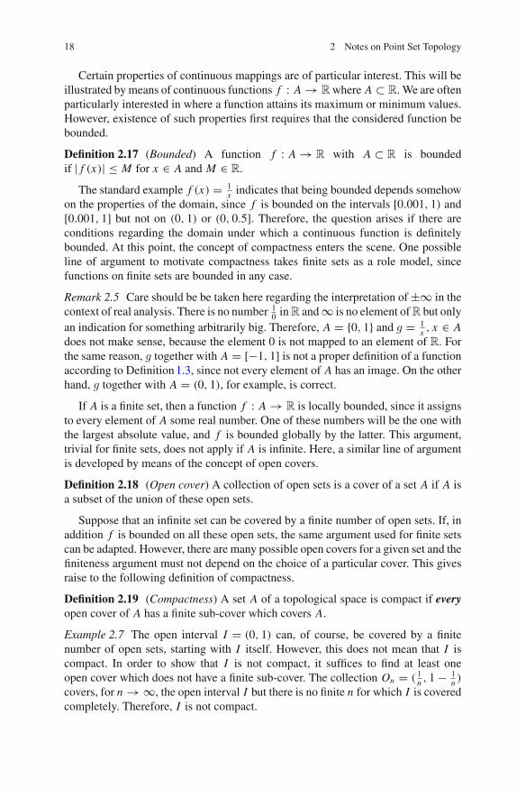
Example 2.7 The open interval I = (0, 1) can, of course, be covered by a finitenumber of open sets, starting with I itself. However, this does not mean that I iscompact. In order to show that I is not compact, it suffices to find at least oneopen cover which does not have a finite sub-cover. The collection On = ( 1n , 1 − 1
n )
covers, for n → ∞, the open interval I but there is no finite n for which I is coveredcompletely. Therefore, I is not compact.

2.4 Connectedness, Compactness, and Separability 19
Of course, to check compactness for a topological space or some subspace bymeans of Definition2.19 might be an option for a mathematician, but will not befor nonmathematicians. However, it turns out that, for instance, all closed intervals[a, b] with a, b ∈ R are compact.
Last but not least, the so-called Hausdorff property ensures that if a sequenceconverges in a topological space X , it converges to exactly one point of X .
Definition 2.20 (Hausdorff) A topological space X is separable or Hausdorff if, forevery x, y ∈ X and x �= y, there exist two disjoint open sets A, B ⊂ X such thatx ∈ A and y ∈ B.
The concept of a basis for a topology is, among other things, useful for checkingif a topological space is a Hausdorff-space.
Definition 2.21 (Basis) Given a topological spaces (X, τ ). A collection τB of ele-ments of τ is called a basis if every member of τ is a union of members of τB .
It can be shown that every space for which a countable basis can be constructedis a Hausdorff-space. All metric spaces in particular fulfill this condition. A possiblebasis for the standard topology in R consists of all open sets (a, b) with a, b ∈ Q,whereQ is the set of rational numbers. SinceQ is countable,R is a Hausdorff-space.
2.5 Product Spaces and Product Topologies
Building a new set X from two sets X1 and X2 bymeans of the Cartesian product, i.e.,X = X1 × X2, is a common and most natural thing to do. If X1 and X2 are equippedwith respective topologies τ1 and τ2, the question about the topology of X inevitablyemerges. Since τ1 is the collection of all open sets in X1 and τ2 is the collection of allopen sets in X2, it seems reasonable to try with the Cartesian product of these sets,specifically to define a collection
B = {U1 ×U2 |U1 ∈ τ1 and U2 ∈ τ2} (2.1)
and to check if B may serve as a topology.
Remark 2.6 In the following, most examples refer to Rn . Since we started with the
intention of working out a minimal structure, suitable for discussing topologicalconcepts, this might seem inconsistent, because Rn has a lot of additional structure.However, R and R
2 especially are quite accessible to our intuition. Furthermore, atopology on a set X can be defined, for instance, by means of a bijective mappingg : X → R
n . Since the existence of a topology is assured inRn , a topology on X canbe defined as the collection of the images g−1(U ) of all open sets U of the standardtopology of Rn . This makes X a topological space and g a continuous mapping.
20 2 Notes on Point Set Topology
X1 = R X1 = R
X2 = R X2 = R
U1U1
U2U2 U1 × U2
W1
W2
(U1 × U2) ∪ (W1 × W2)
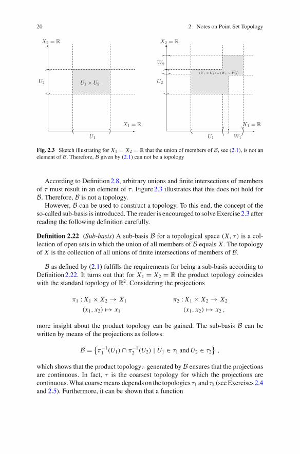
Fig. 2.3 Sketch illustrating for X1 = X2 = R that the union of members of B, see (2.1), is not anelement of B. Therefore, B given by (2.1) can not be a topology
According to Definition2.8, arbitrary unions and finite intersections of membersof τ must result in an element of τ . Figure2.3 illustrates that this does not hold forB. Therefore, B is not a topology.
However, B can be used to construct a topology. To this end, the concept of theso-called sub-basis is introduced. The reader is encouraged to solve Exercise2.3 afterreading the following definition carefully.
Definition 2.22 (Sub-basis) A sub-basis B for a topological space (X, τ ) is a col-lection of open sets in which the union of all members of B equals X . The topologyof X is the collection of all unions of finite intersections of members of B.
B as defined by (2.1) fulfills the requirements for being a sub-basis according toDefinition2.22. It turns out that for X1 = X2 = R the product topology coincideswith the standard topology of R2. Considering the projections
π1 : X1 × X2 → X1 π2 : X1 × X2 → X2
(x1, x2) → x1 (x1, x2) → x2 ,
more insight about the product topology can be gained. The sub-basis B can bewritten by means of the projections as follows:
B = {π−11 (U1) ∩ π−1
2 (U2) | U1 ∈ τ1 andU2 ∈ τ2}
,
which shows that the product topologyτ generated by B ensures that the projectionsare continuous. In fact, τ is the coarsest topology for which the projections arecontinuous.What coarsemeans depends on the topologies τ1 and τ2 (seeExercises2.4and 2.5). Furthermore, it can be shown that a function

2.5 Product Spaces and Product Topologies 21
f : Z → X1 × X2
z → ( f1(z), f2(z) )
is continuous if f1 : Z → X1 and f2 : Z → X2 are continuous, and vice versa.The step toward general finite products, i.e., X1 × X2 × · · · × Xn , is straight
forward. Infinite products, however, require additional considerations.
2.6 Further Reading
A didactic introduction to topology, which nicely illustrates the creativity behind theformal “definition-theorem-proof” structure by showing how the formal language oftopology evolves from first ideas accompanied by trial and error, is given in Geroch[2]. The classic book by Mendelson [4] is a compact and accessible introduction.Also recommendable are Conover [1] and Runde [5], the latter of which also con-tains a number of historical notes. For further steps in topology, we recommend, forexample, Jänich [3]. In addition, summaries of point set topology can be found inmost textbooks on differentiable manifolds.
Exercises
2.1 Check continuity of f in Example2.6 for the following cases:
• f : (X, τ2) → (Y, τ1)• f : (X, τ2) → (Y, τ2)
2.2 Check if (Y, τY )with Y = {a, b} and τY = {∅, {a} , {b}} is a subspace of (X, τX )
with X = {a, b, c, d} and τx = {∅, {a} , {b} , {c} , {d}}.2.3 Given X1 = {0, 1}, X2 = {a, b} together with the topologies τ1 ={X1,∅, {0} , {1}} and τ2 = {X2,∅, {a} , {b}}. Determine the sub-basisB for the prod-uct topology of X = X1 × X2.
2.4 Given X1, X2 and τ1 as in Exercise2.3. Determine the sub-basis B for the topol-ogy τ of X = X1 × X2 for τ2 = {X2,∅}. Determine τ and show that the projectionsare continuous.
2.5 Given X1, X2 and τ2 as in Exercise2.4. Determine the sub-basis B for the topol-ogy τ of X = X1 × X2 for τ1 = {X1,∅}. Determine τ and show that the projectionsare continuous. Compare τ with the corresponding result of Exercise2.4.
22 2 Notes on Point Set Topology
References
1. Conover R (1975) A first course in topology. The Wiliams & Wilkins Company, Baltimore2. Geroch R (2013) Topology. Minkowski Institute Press, Montreal3. Jänich K (1994) Topology. Undergraduate texts in mathematics. Springer, Berlin4. Mendelson B (1975) Introduction to topology. Dover Publications, New York5. Runde V (2000) A taste of topology. Universititext. Springer, Berlin

Chapter 3The Finite-Dimensional Real Vector Space
Abstract The chapter introduces the notion of the finite-dimensional real vectorspace together with fundamental concepts like linear independence, vector spacebasis, and vector space dimension. The discussion of linear mappings between vectorspaces prepares the ground for introducing the dual space and its basis. Finally,inner product space and reciprocal basis are contrasted with dual space and thecorresponding dual basis.
3.1 Definitions
Within the previous chapter, the combination of a set with a topological structurehas been discussed. Now the objective is to discuss a set in combination with analgebraic structure.
Algebraic structures consist of at least one set of objects, also called points in amore general sense, together with a set of operations defined between these objectssatisfying a number of axioms. Specific meanings of objects and operations arecertainly important, for instance, in order to discuss implications of certain results fortechnical applications.On the other hand, abstraction from specific details classifyingproblems by the underlying algebraic structure has proved to be extremely economicand flexible.
Within the hierarchy of algebraic structures, the vector space sits already at arather high level, preceded by the concepts of groups, rings, and fields.
Definition 3.1 (Real vector space) A real vector space V is a set whose elementsare called vectors, for which two binary operations are defined:
1. addition (inner composition “⊕”)The addition of two vectors a and b, a,b ∈ V , is a mapping from V × V to V
⊕ : V × V → V(a,b) �→ a ⊕ b
© Springer International Publishing AG 2017U. Mühlich, Fundamentals of Tensor Calculus for Engineers with a Primeron Smooth Manifolds, Solid Mechanics and Its Applications 230,DOI 10.1007/978-3-319-56264-3_3
23
24 3 The Finite-Dimensional Real Vector Space
with the properties:
(i) a ⊕ b = b ⊕ a(ii) (a ⊕ b) ⊕ c = a ⊕ (b ⊕ c)(iii) there exists a neutral element 0 such that
a ⊕ 0 = a
holds for arbitrary a ∈ V(iv) to every element a, a ∈ V , there exists exactly one element −a, such that
a ⊕ (−a) = 0
holds.
2. multiplication with a real number (outer composition “�”)The multiplication of a vector a ∈ V with a real number α ∈ R is a mapping fromR × V to V
� : R × V → V(α, a) �→ α � a
with the properties:
(I) α � (β � a) = (α β) � a(II) α � (a ⊕ b) = α � a ⊕ α � b(III) (α + β) � a = α � a ⊕ β � a(IV) there exists a neutral element 1, such that
1 � a = a
holds.
The inner composition combines two elements of V , whereas the outer composi-tion combines an element ofV with an element ofR. Both operations are by definitionclosed with respect to V , which means that the result is again an element of V .
The use of⊕ and� indicates that these operations are not necessarily summationand scalar multiplication in the usual sense. On the contrary, they can even meangraphical operations, as defined in the Chap.1.
In the geometrical setting sketched within Chap.1, vectors have been definedby specific properties, namely magnitude and direction. Neither one of these twothings appear in the algebraic definition. On the contrary, specific properties are ofno importance in the algebraic definition but a vector is defined by its behavior underthe considered operations. Furthermore, at this stage, it does not even make sense totalk about a magnitude, because of the lack of a way to measure length, which wouldrequire the definition of a metric first.

3.1 Definitions 25
Be aware that the use of the ordinary “+” on the left-hand side of the thirdproperty of the multiplication is not a mistake, because it expresses the sum of tworeal numbers.
In order to simplify the notation, the “⊕” is often replaced by “+” and λa isused instead of λ � a. This is commonly known as operator overloading.
Remark 3.1 Usually, operator overloading does not cause confusion; however, thereare vector spaces for which it is better to drop this overloading of operation symbolsand to return to the original notation, see, e.g. Exercise3.1. In the follow-up, operationoverloading will be used as long as it does not cause confusion.
Definition3.1 provides the minimal amount of statements necessary to deducethe remaining properties of a vector space by logical reasoning. Two of them are asfollows:
• The neutrals are uniquely determined.• The operations “⊕” and “�” give unique results.
Proving these statements falls under the duties of mathematicians and is beyond thescope here. The interested reader is referred, for example, to Valenza [3].
3.2 Linear Independence and Basis
Definition3.1 provides an abstract frame for vector spaces. On the other hand, theinterpretation of vectors as geometrical objects in the plane, as used in Chap. 1, isactually a particular realization of a vector space. Again, in this context, the additionof vectors and multiplication by scalar are graphical operations. Given a vector a andtwo other vectors g 1 and g 2, and let us assume that
a = a1g 1 + a2g 2 (3.1)
holds, where a1 and a2 are two real numbers. In this context, the superscripts alsomean indices, not powers. The use of upper and lower indices may seem strange atfirst glance, but it provides the possibility of transmitting additional information justby notation. The advantage of this will become clearer later on. Furthermore, let usassume that for another vector b,
b = b1g 1 + b2g 2 (3.2)
holds. According to Definition3.1, the summation of a and b with result c can bewritten as
c = a + b = c1g 1 + c2g 2 (3.3)
26 3 The Finite-Dimensional Real Vector Space
with
c1 = a1 + b1
c2 = a2 + b2 ,
which indicates away to replace the graphical operationswith computations, becausethe real numbers c1 and c2 can be determined just by adding other real numbers.Of course, the result refers to the use of g 1 and g 2. Without this information, thenumbers c1 and c2 are completely meaningless. Obviously, the scheme works onlyif a and b can be expressed by the very same set of vectors {g 1, g 2}. Furthermore,in order for this scheme to be applicable in general, the following questions haveto be answered. Is there always a set of vectors by which every other vector can beexpressed uniquely? Are there always two vectors which have to be chosen for this,and if not, how many are necessary? Can these vectors be chosen arbitrarily, or arethere restrictions? In order to answer these questions, the following definitions arerequired.
Definition 3.2 (Linear independence) N vectors gi , i = 1, . . . , N , gi ∈ V, i ∈ N
are linearly independent if
α1g1 + α2g2 + · · · + αNgN = 0
with αi ∈ R can be fulfilled only by αi = 0, i = 1, . . . , N .
Definition 3.3 (Maximal set of linearly independent vectors) A set consisting ofN vectors {gi }, i = 1, . . . , N , gi ∈ V, i ∈ N is called a maximal set of linearlyindependent vectors if it cannot be extended by any other element of V withoutviolating Definition3.2.
For a finite-dimensional vector space V , the size of all possible maximal setsaccording to Definition3.3 is equal and uniquely determined.
Definition 3.4 (Dimension of a vector space) The dimension of a finite-dimensionalvector space is defined as the size of the sets defined by Definition3.3 and denotedby dim(V).
Before proceeding further, it seems appropriate to do something about notation.Definition3.2 already indicates how tedious notation can become if N is just suffi-ciently large. Of course, the right-hand side in Definition3.2 could be written shorterusing the summation symbol
α1g1 + α2g2 + · · · + αNgN =N∑
i=1
αig i , (3.4)

3.2 Linear Independence and Basis 27
but even this could be dropped if the following conventions, commonly subsumedunder the term Einstein notation, are applied.
Definition 3.5 (Einstein notation) InEinstein notation, indexingobeys the followingrules:
(i) an index appears, at most, twice within a term;(ii) indices which appear only once per term must be the same in every term of an
expression;(iii) if an index appears twice, it must appear exactly once as upper index and once
as lower index, and it indicates that this index is a summation index;(iv) summation indices can be chosen freely as long as this does not conflict with
(i)–(iii).
By employing Einstein notation, the right-hand side of the equation in Definition3.2can be written concisely as αig i without any ambiguity or loss of information. Therange of summation is also clear from the context because it starts with one and theupper range is given by dim(V). An important advantage of such a concise notationis that the structure of a theory or a problem can be apprehended much more easily.Einstein notation is nothing difficult, it only requires some training to get used to it.
Definition 3.6 (Basis of a vector space) Every maximal set of linearly independentvectors according to Definition3.3 forms a basis of the considered vector space. Themembers of such a set are called base vectors.
Based on the two foregoing definitions, answers to the questions raised at thebeginning of this section can be provided.
Every element b of a vector space V can be uniquely represented by a basis{gi } as follows:
b = big i , i = 1, . . . , N
where the bi are called the coordinates or the components of a vector withrespect to the basis {gi }.
A vector space usually has at least dimension one, and it should be noted thatthe zero vector cannot belong to the set of base vectors, since α0 = 0 for anyα ∈ R. On the other hand, the set {0} endowed with vector space operations is alegitimate vector space. Difficulties which may be caused by this are avoided bydefining dim({{0},⊕,�}) = 0.

28 3 The Finite-Dimensional Real Vector Space
3.3 Some Common Examples for Vector Spaces
In the following, some vector spaces are defined which will be used to generateexamples.
Definition 3.7 (The vector spaceR) The set of real numbers, denoted byR togetherwith the usual addition and multiplication defined for real numbers, is a vector space.
Definition 3.8 (The vector space RN ) The elements of RN are all N -tuples of realnumbers
x = (x1, x2, . . . , xN ) ,
for which addition and scalar multiplication are defined as follows:
y + z = (y1 + z1, y2 + z2, . . . , yN + zN )
αy = (αy1,αy2, . . . ,αyN ) ,
with x, y, z ∈ RN ,α, xi , yi ∈ R. Keep in mind that just defining R
N as the set ofall N -tuples of real numbers is not sufficient. RN becomes a vector space only bydefining the respective operations at the same time.
Definition 3.9 (The vector space PM ) The elements of PM are all polynomials oforder M with real coefficients
p(x) = p0 + p1 pow(x, 1) + p2 pow(x, 2) · · · + pM pow(x,M) ,
where pow(x, k) stands for the k-th power of x in order to distinguish powers fromupper indices. Addition and multiplication by scalar are defined by
p(x) + q(x) = (p0 + q0) + (p1 + q1) pow(x, 1) + · · · + (pM + qM) pow(x,M)
λp(x) = λp0 + λp1 pow(x, 1) + · · · + λpM pow(x,M) ,
where, subsequently, pow(x, k) and (x)k are used synonymously. Please note thatdim(PM) = M + 1.
More examples can be found, e.g., in Winitzki [4]. While {(1, 2), (4, 1)} is a suitablebasis for R2, a possible basis for P2 is given by {1, x, (x)2}. Seemingly unrelatedobjects like triples of real numbers and second-order polynomials possess the sameunderlying algebraic structure. This might be surprising at first glance and it alreadygives an idea regarding the power of the vector space concept.
Remark 3.2 RN with N = 2 is a short-hand notation for R × R, which can be
extended easily for arbitrary N ∈ N, as used in Definition3.8. The latter indicateshow new vector spaces can be generated by means of the Cartesian product.

3.4 Change of Basis 29
3.4 Change of Basis
Given a vector space V and a basis {gi }. What happens if we want to use anotherbasis, say {gi }. Besides the importance of this question in general, it is a good startfor practicing the Einstein notation.
Because every element of V can be expressed by means of the basis {gi }, this alsoholds for a vector gi . For dim(V) = 2, we have
g1 = A11 g1 + A2
1 g2
g2 = A12 g1 + A2
2 g2 ,
or for arbitrary dimension using Einstein notation,
gi = Ami gm , (3.5)
where the A ji are real numbers. On the other hand, the gi can be written in terms of
the base vectors gi as follows:
gi = Ami gm . (3.6)
The very same vector v can be expressed using the basis {gi } but also by means of{gi }. The coordinates of both representations will differ, but
vigi = vi gi (3.7)
must hold, because the left- and right-hand sides are just different representationsof the same vector. Evaluating (3.7) by replacing the gi on the right-hand side with(3.5) leads to
vigi − vi Ami gm = 0 . (3.8)
By means of the so-called Kronecker symbol defined by
δji =
{10
ifi = ji �= j
, (3.9)
Equation (3.8) can be written as
[viδmi − vi Am
i
]gm = 0 .
Because the gm are linearly independent, the above equation can be fulfilled onlyif all coefficients are equal to zero. Therefore, the term within the brackets has tovanish, from which
30 3 The Finite-Dimensional Real Vector Space
vm = Ami v
i
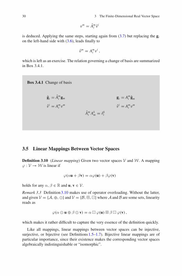
is deduced. Applying the same steps, starting again from (3.7) but replacing the gion the left-hand side with (3.6), leads finally to
vm = Ami v
i ,
which is left as an exercise. The relation governing a change of basis are summarizedin Box 3.4.1.
Box 3.4.1 Change of basis
gi = Ami gm gi = Am
i gm
vi = Ami v
m vi = Ami v
m
Ami A
km = δki
3.5 Linear Mappings Between Vector Spaces
Definition 3.10 (Linear mapping) Given two vector spaces V and W . A mappingϕ : V → W is linear if
ϕ(αu + βv) = αϕ(u) + βϕ(v)
holds for any α,β ∈ R and u, v ∈ V .Remark 3.3 Definition3.10 makes use of operator overloading. Without the latter,and given V = {A,⊕,�} and V = {B,�,�}whereA andB are some sets, linearityreads as
ϕ(α � u ⊕ β � v) = α � ϕ(u) � β � ϕ(v) ,
which makes it rather difficult to capture the very essence of the definition quickly.
Like all mappings, linear mappings between vector spaces can be injective,surjective, or bijective (see Definitions1.5–1.7). Bijective linear mappings are ofparticular importance, since their existence makes the corresponding vector spacesalgebraically indistinguishable or “isomorphic”.

3.5 Linear Mappings Between Vector Spaces 31
Definition 3.11 (Isomorphism) An isomorphism between vector spaces V andW isa bijective linear mapping. Vector spaces for which an isomorphism exists are calledisomorphic, which is denoted by V ∼= W .
Example 3.1 LetV be the vector space of geometric vectors in the plane, as discussedin Sect. 1.2. Although we might have graphical objects in mind, graphical operationscan be replaced by operations with real numbers in R2 simply because V ∼= R
2.
Important properties of a linear mappingϕ follow from its two key characteristics,namely its kernel and its image.
Definition 3.12 (Kernel of a linear mapping) Given two vector spaces V andW anda mapping ϕ : V → W . The kernel of ϕ, denoted by ker ϕ, is the set of all v ∈ Vfor which ϕ(v) = 0 holds, specifically
ker ϕ = {v ∈ V|ϕ(v) = 0}
using set notation.
Definition 3.13 (Image of a linear mapping) Given two vector spaces V andW anda mapping ϕ : V → W . The image of ϕ, denoted by Imϕ, is the set of all w ∈ Wfor which there exist at least one v ∈ W with ϕ(v) = w, specifically
Imϕ = {w ∈ W|w = ϕ(v), v ∈ V}
using set notation.
Considering two vector spaces V and W and a linear mapping ϕ : V → W , theso-called rank-nullity theorem states that
rank ϕ + dim(ker ϕ) = dim(V) , (3.10)
with rank ϕ = dim(Imϕ). Other important facts about linear mappings betweenvector spaces, some of them a direct consequence of (3.10), can be summarized asfollows:
1. Imϕ and ker ϕ are subspaces of their respective vector spaces.2. If dim(ker ϕ) = 0, then ϕ is injective.3. If dim(V) = dim(W), then ϕ is injective if it is surjective, and vice versa, which
implies that finite vector spaces of equal dimensions are isomorphic.4. The inverse of an isomorphism is an isomorphism.
Item one emphasizes the fact that the kernel and image of a linear mapping arenot just subsets of the sets associated with the respective vector spaces but alsovector spaces according to Definition3.1. This has far reaching implications. It canbe used, for instance, to filter out an important or unimportant part, respectively, ofa vector space by means of a linear mapping. The second and third items allow for
32 3 The Finite-Dimensional Real Vector Space
checking the bijectivity of a linear mapping rather easily. Furthermore, item threereveals that all finite-dimensional real vector spaces of dimension N are isomorphicto RN . That vector spaces are algebraically indistinguishable does not mean that thecorresponding operations are equally comfortable to perform (see, e.g., Example3.1).An isomorphism ϕ in the spirit of Example3.1 is really advantageous only, if theresults can be transferred back to the original vector space of interest. This requires theexistence of the inverseϕ−1 and the possibility of derivingϕ−1 explicitly. Fortunately,this is the case which is the essence of item four above. Regarding the respectiveproofs, see, e.g., Axler [1] or Lang [2].
Remark 3.4 The concept of linearity is of outstanding importance. However, aswith most fundamental concepts, the passage from an intuitive understanding to arigorous algebraic definition is by nomeans entirely obvious from the very beginning.Definition3.10 reveals that linearity cannot be definedwithout a notion of summation.In this context, it might be helpful to remember that multiplicationwith a real numberis a generalization of adding things n times, n ∈ N. The reader is encouraged to reviseDefinition3.1 in order to see that it relies entirely on the concept of linearity, andhence vector space is a synonym for linear space.
3.6 Linear Forms and the Dual Vector Space
Definition 3.14 (Linear form) A linear form ω˜is a linear mapping ω
˜: V → R.
The space PM as defined in Definition3.9 with M = 2 is used to discuss theimplications of the concept in more detail. Evaluating the polynomial p(x) ∈ P2
with p(x) = p0 + p1x + p2 (x)2 for some number x
eval x (p(x)) = p0 + p1 x + p2(x)2
is a linear form but also integration with limits
b∫
a
dx(p(x)) = p0[b − a] + p11
2[(b)2 − (a)2] + p2
1
3[(b)3 − (a)3]
and differentiation at some x
d
dx
∣∣∣∣x=x
(p(x)) = p00 + p1 + 2p2 x
are also linear forms over P2. The notation used above differs from the commonnotation for integrals and derivatives in order to stress explicitly that these operationsrequire an argument. Keep in mind that (y)k denotes the k-th power of y.
3.6 Linear Forms and the Dual Vector Space 33
The example illustrates that there are infinitely many linear forms over a givenvector spaceV . Interpreting all these linear forms asmembers of one set, the questionarises as to whether this set possesses an algebraic structure or if some structure canbe imposed on it. As a first step, linearity in Definition3.14 can be explored as
ω˜(v) = ω
˜(vkgk) = vkω
˜(gk) (3.11)
for v ∈ V and some basis {gi } of V . Since the ω˜(gk) have to be real numbers,
ωk = ω˜(gk)
is used in the following. Hence, (3.11) reads as
ω˜(v) = vkωk ,
and the following observations can be made. First of all, any linear form can berepresented by a sum of N products, where N = dim(V). Furthermore, differentlinear forms are obviously represented by different values for the ωi and the questionarises as to whether these representations are unique. In other words, can the samelinear form be represented by more than one set of coefficients? Considering twolinear forms ω
˜and η
˜, ω˜(v) = η
˜(v) leads to
vkωk = vkηk
and
vk[ωk − ηk] = 0 ,
respectively. Since this holds for any v ∈ V , two linear forms are equal only if theirrespective coefficients are equal. This, on the other hand, implies that the represen-tation of a linear form ω
˜by the numbers ωi is unique.
The next step consists in considering particular linear forms, namely those whichread of the j-th component of a given vector. For reasons which will become clearlater, we denote these linear forms by g
˜j , and
g˜
j (v) = v j (3.12)
defines them explicitly. Using (3.12) in (3.11) reads as
ω˜(v) = ωk g
˜k(v) , (3.13)
the implications of which are illustrated for dim(V) = 2. In this case, (3.13) readsas
ω˜(v) = ω1 g
˜1(v) + ω2 g
˜2(v) , (3.14)

34 3 The Finite-Dimensional Real Vector Space
which in view of Sect. 3.2 indicates that the linear forms over V might form a vectorspace. In order to exploit this idea further, the forms have to be separated from theirarguments. This, on the other hand, requires defining a summation of linear formsindirectly by means of (3.14). This also has to be done for multiplication of a linearform with a real number and is part of the following definition.
Definition 3.15 (Dual space) The set of all linear forms over a vector space V ,together with two operations “⊕” and “�”, is called the dual space of V and denotedby V∗. The operations are defined according to
[ω˜
⊕η˜
](v) = ω
˜(v) + η
˜(v) (3.15)
[λ�ω
˜](v) = ω
˜(λv) , (3.16)
and the elements of V∗ are called co-vectors or dual vectors, respectively.
The meaning of the operations “⊕” and “�” depends on V . It is important in thefollowing to distinguish between the mapping itself and the result when evaluatedfor the respective argument. That
dim(V) = dim(V∗)
is clear due to the observation discussed after (3.11) together with (3.13). Further-more, (3.12) implies that
g˜i (g j ) = δij
and the g˜i are called dual base vectors. Here, the advantage of using the index
positions in order to transmit additional information by notation becomes apparent.That the index position alone is not sufficient to distinguish between base vectorsand dual base vectors is due to the existence of the so-called reciprocal basis whichwill be discussed later.
In the following, the notations ω˜
+ ν˜
:= ω˜
⊕ν˜and λω
˜:= λ�ω
˜are used as
long as this operator overloading does not cause confusion.
The properties of ω˜(v) (see (3.11)) suggest an alternative notation which empha-
sizes the pairing of a vector and a co-vector
⟨ω˜, v
⟩ := ω˜(u) , (3.17)
where⟨ω˜, v
⟩is called dual product since it is distributive regarding addition defined
for V and V∗. The coordinates of vectors and dual vectors can be expressed by meansof (3.17), and the corresponding base vectors as
3.6 Linear Forms and the Dual Vector Space 35
vi =⟨g˜i , v
⟩(3.18)
ωi = ⟨ω˜, gi
⟩, (3.19)
which will be used extensively in the follow-up.
Example 3.2 Let V = P2 with {g i } = {1, x, (x)2}. The corresponding dual basis isgiven by
{eval 0, d
dx
∣∣0, (d)2
d(x)2
∣∣∣0
}.
Remark 3.5 (Importance of the dual space in mechanics) Imagine the state of asystem is described by a scalar function, e.g., work which depends on the actualposition expressed by a vector x(τ ) where τ stands for time. Derivative of W wrt.time at a specific time t leads to the concept of power, which is actually a linearizationconcept. Although derivatives are not discussed more rigorously until Chap. 6, it isclear from previous education in analysis that a kind of chain rule will be involvedby which the vector x(t) appears. The result of the time derivative is a real number,obtained by pairing the vector x(t) with something else, hence
W (x(t) ) =⟨dW
dx
∣∣∣∣x(τ=t)
, x(t)
⟩.
If x is a vector paired with something and the result is a real number, then dWdx
∣∣x(τ=t)
is a co-vector. In mechanics, dWdx
∣∣x(τ=t)
is interpreted as a force. Nowadays, it istherefore understood that forces should be encoded mathematically as dual vectorsrather than as vectors.
3.7 The Inner Product, Norm, and Metric
Definition 3.16 (Inner product) A mapping
· : V × V → R
(a,b) �→ a · b
with the properties:
(i) a · b = b · a(ii) (αa + βb) · c = αa · c + βb · c(iii) a �= 0 ⇒ a · a > 0
for all a,b, c ∈ V und α,β ∈ R is called an inner product. A vector space equippedwith an inner product is called an inner product space or pre-Hilbert space.
Example 3.3 Here again, definitions are derived from studying different situationsand extracting common patterns. This leads eventually to definitions providing aminimum amount of information from which other facts can be deduced by logical

36 3 The Finite-Dimensional Real Vector Space
reasoning. For instance, that for v �= 0, u · v = 0 implies u = 0 is not part of thedefinition. However, using the fact that u + 0 = u leads to
u · v + 0 · v = 0 .
Since u ·v = 0, the only inner product involving v which evaluates to zero is the onewith the zero vector. Hence, u = 0.
According to Definition3.16, the inner product u · v with u, v ∈ V takes twoarguments and it is linear in both. This is referred to as bilinear mapping. If oneargument is fixed, e.g., u = u, then the inner product becomes a linear form. Becausethe dual space V∗ is the space of all linear forms, there has to be a correspondingdual vector η
˜∈ V∗ by which exactly the same result can be obtained, specifically
⟨η˜, v
⟩= u · v .
In other words, a mapping
G : V → V∗ (3.20)
u �→ η˜
= G(u)
must exist such that⟨G(u), v
⟩= u · v . (3.21)
Linearity of G is implied by the linearity of the inner product together withDefinition3.15. Bijectivity follows from ker G = 0
˜and dim(V) = dim(V∗). There-
fore, the inner product induces an isomorphism between V andV∗ (see also Exer-cise3.4).
The importance of the inner product consists in the fact that it induces a norm.The latter is a generalization of measuring length.
Definition 3.17 (Norm) A norm ||.|| on a vector space V is a mapping with theproperties:
(i) ||αv|| = α||v||(ii) ||u + v|| ≤ ||u|| + ||v||(iii) ||v|| = 0 implies u = 0
for α ∈ R and u, v ∈ V .The norm of a vector u induced by the inner product is simply
||u|| = √u · u ,
and a norm on the other hand induces a metric by means of the distance function

3.7 The Inner Product, Norm, and Metric 37
d(u, v) = ||u − v||
(see also Definition2.1). Therefore, V becomes a metric space in the presence of aninner product.
3.8 The Reciprocal Basis and Its Relations with the DualBasis
Definition 3.18 (Reciprocal basis) Given a vector space V with inner product andsome basis {gi }. The reciprocal basis {gi } is defined by
gi · g j = δji
with gi , g j ∈ V .
Box 3.8.1 Relation between inner product and dual product
vector space V
u ∈ Vbasis {g i }
ω˜
: V → R
common notations (α ∈ R):
α = ω˜(u)
α = ⟨ω˜,u
⟩
or even
α = ω˜
· u
dual space V∗
ω˜
∈ V∗
basis {g˜i }
If V is an inner product space then the reciprocal basis {g j } is defined byg i · g j = δ
ji . Furthermore,
⟨g˜i , v
⟩= gi · v
holds.
38 3 The Finite-Dimensional Real Vector Space
Using the knowledge of the previous subsection about the isomorphism estab-lished by the existence of an inner product,
⟨G(gi ), v⟩ = gi · (vkgk) = gi · gkvk = vi (3.22)
where the properties of the reciprocal basis were used. On the other hand,
⟨g˜i , v
⟩= vi (3.23)
holds, and comparison of (3.22) with (3.23) yields
G(gi ) = g˜i ,
from which⟨g˜i , v
⟩= gi · u (3.24)
can be deduced. This does not mean that dual basis and reciprocal basis are the
same thing. It just means that⟨g˜i ,u
⟩could be replaced by gi · u because it gives the
same result, the same real number, to be precise. The relations between inner productand dual product are summarized in Box 3.8.1 together with notations commonlyemployed for the dual product.
Remark 3.6 The result (3.24) is often used to abandon the concept of the dual spacecompletely, which is by no means a good idea, because most of the underlyinginformation becomes invisible without getting any benefit in exchange.
In the presence of an inner product, the so-called metric coefficients gi j and gi j
can be defined by
gi j = gi · g j (3.25)
gi j = gi · g j , (3.26)
which will play an important role later. A basis {Ei } with the property
Ei · E j ={10
ifi = ji �= j
.
is called orthonormal. In this case, base vectors and reciprocal vectors coincide. Thissubject will be enlarged upon later (see Sect. 6.3).
Exercises
3.1 Show that the set of all positive real numbers R+
R+ := {x | x ∈ R and x > 0}

3.8 The Reciprocal Basis and Its Relations with the Dual Basis 39
together with the operations
a ⊕ b := a · bλ � a := aλ
with a, b ∈ R+,λ ∈ R forms a real vector space. Hints: show that R+ is closed
under the given operations and that the operations obey the rules defined for vectorspaces. Furthermore, determine explicitly the neutral element for the operation ⊕,the neutral element for the operation � and the inverse with respect to the operation⊕.
3.2 Consider V = R2. The elements of V are pairs of real numbers, e.g., (x1, x2).
Choose g 1 and g 1 and deduce the meanings of ⊕ and ⊗ for this case.
3.3 Determine the transformation relationship for the dual base vectors in case of achange of basis (see Box 3.4.1).
3.4 Show that G as defined by (3.20) and (3.21) is an isomorphism.
3.5 Show that1∫
0dx p(x)q(x) is a suitable definition for an inner product in P2.
3.6 Evaluate explicitly δii , δii δ
jj , and δ
ji δ
ij for i, j, k = 1, 2, 3.
3.7 Simplify Akjδ
jk , δ
ji δ
kj , and δ
ji A j − δki Ak .
3.8 Given the space W = V∗ × V with elements (ω˜,u) where ω
˜∈ V∗,u ∈ V . W
becomes a vector space by defining
(ω˜,u) ⊕ (ν
˜, v) = (ω
˜+ ν
˜,u + v) ,
λ � (ω˜,u) = (λω
˜,λu)
with λ ∈ R, v ∈ V,ν˜
∈ V∗. Show that dim(V) = 3 implies dim(W) = 6.
Hint: Since (ω˜,u) = ωiv
k(g˜i , gk), the question can be answered by determining the
number of linearly independent pairs (g˜i , gk).
3.9 Given a vector space V with inner product. Use the relationship
gi · g j ≡ δj
i (gi , g j ∈ V)
1. to determine the component matrix Bi j for the basis transformation gi = Bi j g j ,
2. to prove the identity gik gk j = δj
i where the gi j := gi · g j and gi j := gi · g j arethe so-called metric coefficients.

40 3 The Finite-Dimensional Real Vector Space
References
1. Axler S (2010) Linear algebra done right. Undergraduate texts in mathematics. Springer, Berlin2. Lang S (1997) Introduction to linear algebra. Undergraduate texts in mathematics. Springer,
Berlin3. Valenza R (1993) Linear algebra: an introduction to abstract mathematics. Undergraduate texts
in mathematics. Springer, Berlin4. Winitzki S (2010) Linear algebra via exterior products. www.lulu.com

Chapter 4Tensor Algebra
Abstract Dyadic product and tensors are introduced in the context of bilinear formsbefore extending this scheme to arbitrary but finite dimensions. Afterwards, tensorproduct spaces are defined. The exterior product is motivated within this chapter bythe aim to generalize the notion of volume for arbitrary dimensions and to overcomethe limitations implied by the cross product of conventional vector calculus. Withinthis context, symmetric and skew-symmetric tensors, as well as a generalized versionof the Kronecker symbol, are discussed. Furthermore, basic aspects of the so-calledstar-operator are examined. The latter relates spaces of alternating tensors of equaldimension based on the existence of an inner product.
4.1 Tensors and Multi-linear Forms
The coordinate representation of tensors involves systematic indexing, which makesthe use of tensors of arbitrary order somewhat difficult at the beginning. Hence, thefundamental relations will be derived first for second order tensors.
Consider the vector space V and its dual V∗ without any inner product togetherwith the following linear mapping:
A : V∗ × V → R . (4.1)
Due to the linearity, applying the mapping A for two particular arguments ω˜
∈ V∗and v ∈ V reads as
α = A(ω˜
, v) = ωivj A(g
˜
i , g j ) , (4.2)
where α is the result of the operation, and according to the definition above, α ∈ R.Because the objects on both sides of (4.2) have to be real numbers, the A(g
˜
i , g j )
must be real numbers. If the abbreviation
Aij = A(g
˜
i , g j )
© Springer International Publishing AG 2017U. Mühlich, Fundamentals of Tensor Calculus for Engineers with a Primeron Smooth Manifolds, Solid Mechanics and Its Applications 230,DOI 10.1007/978-3-319-56264-3_4
41
42 4 Tensor Algebra
is used, (4.2) can be written as
α = A(ω˜
, v) = Aij ωi v
j ,
and it can be shown that the right hand side is invariant under a change of basis, whichis left as an exercise to the reader. Again, the idea is to isolate themapping (operation)from its arguments. This can be done by means of the dual product, which can beused to read off the coordinates of a vector or a covector, respectively. Applicationof (3.18) and (3.19) yields
A(ω˜
, v) = Aij
⟨
ω˜
, gi
⟩
⟨
g˜
i , v⟩
. (4.3)
The term⟨
ω˜
, gi⟩
⟨
g˜
i , v⟩
is a bilinear form itself and written symbolically as
⟨
ω˜
, gi⟩
⟨
g˜
i , v⟩
= gi ⊗ g˜
j (ω˜
, v) , (4.4)
where “⊗” is the so-called dyadic product. The mapping (4.1) can therefore berepresented by the object
A = Aij gi ⊗ g
˜
j ,
and A(ω˜
, v) again yields (4.3) if the definition (4.4) is used. A is called a secondorder tensor.
Of course, the right hand side of (4.3) consists of real numbers, the order of whichcan be chosen arbitrarily. However, here the convention is used that the order of thearguments according to the definition (4.1) determines the order of the base vectorsand dual base vectors, respectively, such that the n-th argument meets the n-th basevector or dual base vector. As long as no inner product is defined for V , the operationcan be performed only if a vector argument meets a dual base vector, and vice versa.
Obviously, this scheme can be used to encode other possible bilinear forms. Theresults are summarized as follows:
A : V∗× V → R A = Aij gi⊗g
˜
j
B : V × V → R B = Bi j g
˜
i⊗g
˜
j
C : V × V∗→ R C = C ji g
˜
i⊗g j
D : V∗× V∗→ R D = Di j gi⊗g j .
Remark 4.1 Regarding the RHS of (4.4), the notation gi g˜
j (ω˜
, v) might seemmore natural at this point, and, in fact, it can be found in the literature as well. Theappearance of ⊗ in (4.4) and calling gi ⊗ g
˜
j a product is justified by the distributiveproperty of this construction, to be discussed in more detail later.
4.1 Tensors and Multi-linear Forms 43
The generalization from bilinear forms discussed above to multi-linear forms isstraight forward.
Definition 4.1 (Tensor as multi-linear form) A tensor T(nm)
is a mapping
T(mn): V∗ × · · · × V∗︸ ︷︷ ︸
m-times
×V × · · · × V︸ ︷︷ ︸
n-times
→ R , (4.5)
which is linear in all of its arguments.
Since m and n can be arbitrary natural numbers, it is advisable to work with so-called multi-indices. This will be illustrated by means of a T(22)
tensor. T(22)can be
expressed byT(22)
= T i jkl gi ⊗ g j ⊗ g
˜
k ⊗ g˜
l . (4.6)
Performing the replacements
i → i1 , j → i2 , k → j1 , l → j2 , (4.7)
T(22)reads as
T(22)= T i1i2
j1 j2gi1 ⊗ gi2 ⊗ g
˜
j1 ⊗ g˜
j2 .
As long as m and n are small, a representation like the one in (4.6) is preferable.However, form, n large or arbitrary, the following representation of the tensor relatedto Definition4.1 is possible:
T(mn)= T i1...im
j1... jngi1 · · · ⊗ · · · gim ⊗ g
˜
j1 · · · ⊗ · · · g˜
jn .
Definition4.1 considers only a vector spaceV and its dual. However, more generalcases are not only possible but also rather important. Therefore, more general settingsare also discussed subsequently.
4.2 Dyadic Product and Tensor Product Spaces
The intention of the following discussion is to generalize the operation “⊗”, whichfirst appeared in the definition of the dyadic product (4.4),
gi ⊗ g˜
j (ω˜
, v) = ⟨
ω˜
, gi⟩
⟨
g˜
i , v⟩
,
with gi ∈ V, g˜
i ∈ V∗, for arbitrary elements of V and V∗.The dual product is a linear mapping, hence (4.4) is a bilinear mapping, meaning
linear in both arguments. Because the gi and g˜
j are themselves just vectors and dualvectors, (4.4) is adapted as follows:

44 4 Tensor Algebra
u ⊗ η˜
(ω˜
, v) = uiηk gi ⊗ g˜
k (ω˜
, v) ,
which indicates that “⊗” can be defined in a more general way that includes (4.4).
Definition 4.2 (Tensor space V ⊗ W) Given two vector spaces V and W withdim(V) = N , dim(W) = K . The tensor product space V ⊗ W is defined by thefollowing properties:
(i) There exists a mapping “⊗” called tensor product or dyadic product such that
⊗ : V × W → V ⊗ W(u,W) �→ u ⊗ W .
(ii) If {gi } is a basis of V and {Gi } a basis of W , then the {gi ⊗G j } form a basis ofV ⊗ W . Every element T of V ⊗ W can therefore be expressed by
T = T i jgi ⊗ G j .
(iii) Summation and multiplication with scalar are defined for V ⊗ W by
A + B = [Ai j + Bi j ]gi ⊗ G j
λA = λAi jgi ⊗ G j .
(iv) The mapping “⊗” has the following properties:
u ⊗ (V + W) = u ⊗ V + u ⊗ W
(u + v) ⊗ W =u ⊗ W + v ⊗ W
(λu) ⊗ W =u ⊗ (λW) = λ(u ⊗ W) ,
with u, v ∈ V,V,W ∈ W , λ, T i j ∈ R, and i = 1 . . . N , j = 1 . . . K .
Due to (iii), V ⊗ W is a vector space. Obviously, v ⊗ W, v ∈ V,W ∈ W is anelement of V ⊗ W . However, not all elements of V ⊗ W are of this form. This canbe seen easily through simple examples (see Exercise4.3).
Remark 4.2 Without operator overloading, (iv) ofDefinition4.2would take the form
u ⊗ (V � W) = u ⊗ V�u ⊗ W
(u ⊕ v) ⊗ W = u ⊗ W�v ⊗ W
(λ � u) ⊗ W = u ⊗ (λ � W) = λ�(u ⊗ W)
for {V,⊕,�}, {W,�,�}, and {V ⊗ W, �, �}, which makes it hardly readable.
Defining the spaces V ⊗ W∗, W∗ ⊗ V , etc., works analogously to Definition4.2.Furthermore, the tensor space concept can be generalized in a straightforwardmannerfor dyadic products of more than two vector spaces.

4.2 Dyadic Product and Tensor Product Spaces 45
The tensor space V ⊗ V can be written more concisely as ⊗2V . If the tensorproduct is applied k times, then ⊗kV is commonly used for the corresponding tensorspace.
In order to illustrate the relation between multi-linear forms and tensor productspaces, the bilinear form
F : V∗ × W → R , (4.8)
which corresponds toF = F j
i G j ⊗ g˜
i , (4.9)
is considered together with a mapping ϕ : W ⊗ V∗ → R. Evaluating ϕ with respectto the argument Ω
˜
⊗ v and standard manipulation yields
ϕ(Ω˜
⊗ v) = Ωi vkϕ(G˜
i ⊗ gk) = Φ ik Gi ⊗ g
˜
k(Ω˜
, v) ,
which shows thatϕ can be converted into a bilinear form similar toF in (4.8). Feedingϕ and F with the same arguments gives equal results if
F ji = Φ
ji (4.10)
holds. Since (4.10) has a unique solution for either F orΦ given, there exists a uniqueϕ for every F. This is a particular case reflecting the so-called universal property ofthe tensor product illustrated in Fig. 4.1. It justifies a definition of a tensor as an objectin its own right, i.e., as an element of a tensor product space
T(mn)∈ W ⊗ · · · ⊗ W
︸ ︷︷ ︸
m-times
⊗ V∗ ⊗ · · · ⊗ V∗︸ ︷︷ ︸
n-times
. (4.11)
Equivalence with Definition4.1 is ensured by the universal property.Definition4.2 relies on the existence of a basis. Once the construction of the
tensor space is established, it can be shown that this construction is independent ofa particular choice for a basis by means of the transformation properties of tensors.
Fig. 4.1 Commutativediagram illustrating theuniversal property of thetensor product
V∗ × W
W ⊗ V∗
R
F
ϕ
⊗

46 4 Tensor Algebra
Alternatively, basis-free constructions can be performed, an action which has theadvantage that a tensor product can be established for arbitrary sets that might noteven have a basis. However, these constructions are more involved and work viathe notion of the free vector space and an appropriate quotient space. The interestedreader is referred, e.g., to Lee [2].
As long as all involved vector spaces have the same dimension, which is often thecase, the universal property ensures that it is sufficient to define tensors by Defini-tion4.1, since by choosing one vector space as V , all others can be related to V byproper isomorphisms.
4.3 The Dual of a Linear Mapping
The dual A∗ of a linear mapping A : V → W is defined as follows:
⟨
Ω˜
,A(v)⟩ = ⟨
A∗(Ω˜
), v⟩
, (4.12)
with v ∈ V and ω ∈ V∗. Since the dual product is only defined between a vectorspace and its own dual space, A∗ has to be a mapping
A∗ : W∗ → V∗ .
Using the bases {gi } ∈ V and {Gi } ∈ W together with their duals, A and A∗ read as
A = Aik Gi ⊗ g
˜
k
A∗ = A∗ik g˜
k ⊗ Gi ,
and direct evaluation of (4.12) yields
Aik = A∗i
k .
While the linear mapping A : V → W establishes a relation between two vectorspaces, its dual establishes a corresponding relation between the respective dualspaces.
4.4 Remarks on Notation and Inner Product Operations
Regarding the notation employed so far, there is not much space for ambiguity.GivenT(01)
(u),T(11)(u) orT(02)
(u), Definition4.1 or (4.11) indicate the correspondingoperations

4.4 Remarks on Notation and Inner Product Operations 47
T(01)(u) = Tig
˜
i (ukgk) = Tiui
T(11)(u) = T j
i g j ⊗ g˜
i (ukgk) = T ji u
ig j
T(02)(u) = Ti jg
˜
i ⊗ g˜
j (ukgk) = Ti j ujg˜
i ,
but an expression like T(u), for instance, does not provide sufficient information. Itis also clear that T(10)
(u) and T(20)(u) do not make sense because the dual product is
defined for a dual vector paired with a vector.If, however, dual vectors are replaced by reciprocal vectors and operations are
expressed by means of the inner product, additional conventions are commonlyintroduced in order to avoid ambiguity. Of course, this is only possible for innerproduct spaces. Since in
T ji g j ⊗ gi · (ukgk) , (4.13)
g j · gk as well as gi · gk make sense, it has to be agreed upon as to how the operationshould be performed. Furthermore, inner products of arbitrary order, e.g., a doubleinner product A · ·B, can be defined. Here, we define for a single inner productbetween two tensors that the last vector/reciprocal vector of the first tensor meetsthe first vector/reciprocal vector of the second tensor. Furthermore, a multiple innerproduct proceeds to the left regarding the first tensor and to the right with respect tothe second tensor. For example,
T(11)· u = T j
i ukg j (gi · gk) = T j
i uig j
T(20)· u = T i j ukgi (g j · gk) = T j
i uig jk gi
T(11)· ·T(20)
=[
T ji g j ⊗ gi
]
· · [T kl gk ⊗ gl] = T j
i Tikg jl ,
where the gi j are the metric coefficients discussed in Sect. 3.8. Please note that otherconventions are also possible, and used in the literature.
Two very common operations when working with inner product spaces and usingthe reciprocal basis instead of the dual basis are raising and lowering indices. Avector u can be expressed either by {gi } or
{
gi}
. Taking the inner product of bothsides of
ui gi = uk gk
with gl and gl , respectively, yields
ul = ukgkl , ul = ukgkl ,
which means that
u = uk gk = ukgkl gl = ukgkl gl = uk gk .
This scheme extends in a straightforward manner to tensors of arbitrary order.
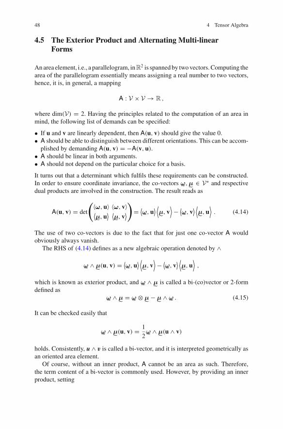
48 4 Tensor Algebra
4.5 The Exterior Product and Alternating Multi-linearForms
Anarea element, i.e., a parallelogram, inR2 is spanned by twovectors. Computing thearea of the parallelogram essentially means assigning a real number to two vectors,hence, it is, in general, a mapping
A : V × V → R ,
where dim(V) = 2. Having the principles related to the computation of an area inmind, the following list of demands can be specified:
• If u and v are linearly dependent, then A(u, v) should give the value 0.• A should be able to distinguish between different orientations. This can be accom-plished by demanding A(u, v) = −A(v,u).
• A should be linear in both arguments.• A should not depend on the particular choice for a basis.
It turns out that a determinant which fulfils these requirements can be constructed.In order to ensure coordinate invariance, the co-vectors ω
˜
,μ˜
∈ V∗ and respectivedual products are involved in the construction. The result reads as
A(u, v) = det
(〈ω˜
,u〉 〈ω˜
, v〉⟨
μ˜
,u⟩ ⟨
μ˜
, v⟩
)
= ⟨
ω˜
,u⟩
⟨
μ˜
, v⟩
− ⟨ω˜
, v⟩
⟨
μ˜
,u⟩
. (4.14)
The use of two co-vectors is due to the fact that for just one co-vector A wouldobviously always vanish.
The RHS of (4.14) defines as a new algebraic operation denoted by ∧
ω˜
∧ μ˜
(u, v) = ⟨
ω˜
,u⟩
⟨
μ˜
, v⟩
− ⟨ω˜
, v⟩
⟨
μ˜
,u⟩
,
which is known as exterior product, and ω˜
∧ μ˜
is called a bi-(co)vector or 2-formdefined as
ω˜
∧ μ˜
= ω˜
⊗ μ˜
− μ˜
∧ ω˜
. (4.15)
It can be checked easily that
ω˜
∧ μ˜
(u, v) = 1
2ω˜
∧ μ˜
(u ∧ v)
holds. Consistently, u ∧ v is called a bi-vector, and it is interpreted geometrically asan oriented area element.
Of course, without an inner product, A cannot be an area as such. Therefore,the term content of a bi-vector is commonly used. However, by providing an innerproduct, setting
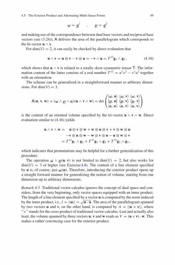
4.5 The Exterior Product and Alternating Multi-linear Forms 49
ω˜
= g˜
1 , μ˜
= g˜
2
and making use of the correspondence between dual base vectors and reciprocal basevectors (see (3.24)), A delivers the area of the parallelogram which corresponds tothe bi-vector u ∧ v.
For dim(V) = 2, it can easily be checked by direct evaluation that
u ∧ v = u ⊗ v − v ⊗ u = −v ∧ u = T 12g1 ∧ g2 , (4.16)
which shows that u ∧ v is related to a totally skew-symmetric tensor T. The infor-mation content of the latter consists of a real number T 12 = u1v2 − v1u2 togetherwith an orientation.
The scheme can be generalized in a straightforward manner to arbitrary dimen-sions. For dim(V) = 3,
A(u, v,w) = (ω˜
∧ μ˜
∧ κ˜
)(u ∧ v ∧ w) = det
⎛
⎝
〈ω˜
,u〉 〈ω˜
, v〉 〈ω˜
, v〉⟨
μ˜
,u⟩ ⟨
μ˜
, v⟩ ⟨
μ˜
, v⟩
〈κ˜
, u〉 〈κ˜
, v〉 〈κ˜
, v〉
⎞
⎠
is the content of an oriented volume specified by the tri-vector u ∧ v ∧ w. Directevaluation similar to (4.16) yields
u ∧ v ∧ w = u ⊗ v ⊗ w + w ⊗ u ⊗ v + v ⊗ w ⊗ u
−v ⊗ u ⊗ w − w ⊗ v ⊗ u − u ⊗ w ⊗ v
= T 12g1 ∧ g2 + T 13g1 ∧ g3 + T 23g2 ∧ g3 ,
which indicates that permutations may be helpful for a further generalization of thisprocedure.
The operation ω˜
∧ μ˜
(u, v) is not limited to dim(V) = 2, but also works fordim(V) = 3 or higher (see Exercise4.8). The content of a line element specifiedby u is, of course, just ω
˜
(u). Therefore, introducing the exterior product opens upa straight forward manner for generalizing the notion of volume, starting from onedimension up to arbitrary dimensions.
Remark 4.3 Traditional vector calculus ignores the concept of dual space and con-siders, from the very beginning, only vector spaces equipped with an inner product.The length of a line element specified by a vector u is computed by the norm inducedby the inner product, i.e., l = ||u|| = √
u · u. The area of the parallelogram spannedby two vectors u and v, on the other hand, is computed by A = ||u × v||, where“×” stands for the cross product of traditional vector calculus. Last and actually alsoleast, the volume spanned by three vectors u, v andw reads as V = (u× v) ·w. Thismakes a rather convincing case for the exterior product.

50 4 Tensor Algebra
According to Sect. 3.6, a dual vector ω˜
is a linear form. Consistently, ω˜
∧ η˜
iscommonly called an alternating 2-form or just a 2-form. This scheme extends in astraightforward manner to n-forms.
This section indicates distinctly that a more general treatment of skew-symmetrictensors is necessary, which implies the need to consider symmetric tensors as well.
4.6 Symmetric and Skew-Symmetric Tensors
The following definitions refer to the definition of tensors in the context of multi-linear forms (see Definition4.1).
Definition 4.3 (Symmetric tensors) A T(m0)tensor is symmetric with respect to its
k th and l th argument if
α = T(m0)(. . . ,
(k)v , . . . ,
(l)v , . . .) = T(m0)
(. . . ,(l)v , . . . ,
(k)v , . . .)
holds. T(m0)is totally symmetric if, for every possible permutation of its arguments,
α remains unchanged. Analogously, a T(0n)tensor is symmetric with respect to its k th
and l th argument if
α = T(0n)(. . . ,
(k)ω˜
, . . . ,(l)ω˜
, . . .) = T(0n)(. . . ,
(l)ω˜
, . . . ,(k)ω˜
, . . .)
holds. T(0q)is totally symmetric if, for every possible permutation of its arguments,
α remains unchanged.
Definition 4.4 (Skew-symmetric tensors) A T(0n)tensor is skew symmetric with
respect to its k th and l th argument if
T(0n)(. . . ,
(k)ω˜
, . . . ,(l)ω˜
, . . .) = −T(0n)(. . . ,
(l)ω˜
, . . . ,(k)ω˜
, . . .)
holds. It is totally skew symmetric if
T(0n)((i1)ω˜
,(i2)ω˜
, . . . ,(in)ω˜
) = q T(0n)(( j1)ω˜
,( j2)ω˜
, . . . ,( jn)ω˜
)
with
q =⎧
⎨
⎩
−1 an oddfor j1 j2 . . . jn distinct and permutation of i1 i2 . . . in
1 an even,
and q = 0 otherwise, holds. Skew-symmetry of a T(m0)tensor is defined analogously.
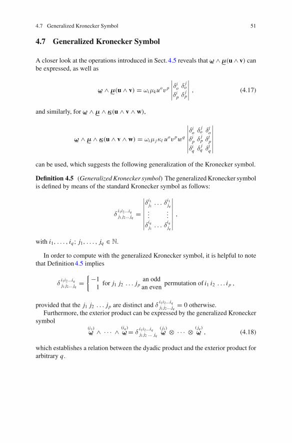
4.7 Generalized Kronecker Symbol 51
4.7 Generalized Kronecker Symbol
A closer look at the operations introduced in Sect. 4.5 reveals that ω˜
∧ μ˜
(u∧ v) canbe expressed, as well as
ω˜
∧ μ˜
(u ∧ v) = ωiμkuov p
∣
∣
∣
∣
∣
δio δjo
δip δjp
∣
∣
∣
∣
∣
, (4.17)
and similarly, for ω˜
∧ μ˜
∧ κ˜
(u ∧ v ∧ w),
ω˜
∧ μ˜
∧ κ˜
(u ∧ v ∧ w) = ωiμ jκl uov pwq
∣
∣
∣
∣
∣
∣
∣
δio δjo δlo
δip δjp δlp
δiq δjq δlq
∣
∣
∣
∣
∣
∣
∣
can be used, which suggests the following generalization of the Kronecker symbol.
Definition 4.5 (GeneralizedKronecker symbol) The generalizedKronecker symbolis defined by means of the standard Kronecker symbol as follows:
δi1i2...iqj1 j2... jq
=
∣
∣
∣
∣
∣
∣
∣
∣
δi1j1 . . . δi1jq...
...
δiqj1
. . . δiqjq
∣
∣
∣
∣
∣
∣
∣
∣
,
with i1, . . . , iq; j1, . . . , jq ∈ N.
In order to compute with the generalized Kronecker symbol, it is helpful to notethat Definition4.5 implies
δi1i2...iqj1 j2... jq
={−1
1for j1 j2 . . . jp
an oddan even
permutation of i1 i2 . . . i p ,
provided that the j1 j2 . . . jp are distinct and δi1i2...iqj1 j2... jq
= 0 otherwise.Furthermore, the exterior product can be expressed by the generalized Kronecker
symbol(i1)ω˜
∧ · · · ∧ (iq )ω˜
= δi1i2...iqj1 j2 ... jq
( j1)ω˜
⊗ · · · ⊗ ( jq )ω˜
, (4.18)
which establishes a relation between the dyadic product and the exterior product forarbitrary q.

52 4 Tensor Algebra
4.8 The Spaces ΛkV and ΛkV∗
The totally skew-symmetric tensors of a tensor space form a linear subspace ofparticular interest. In order to explore this, totally skew-symmetric projections arefirst discussed for the spaceV⊗V . In this context, a totally skew-symmetric projectionis a linear mapping
P : V ⊗ V → V ⊗ V (4.19)
B �→ C = P(B)
with the properties
P(C) = C (4.20)
C(ω˜
,η˜
) = −C(η˜
,ω˜
) , (4.21)
withω˜
,η˜
∈ V∗. Property (4.20) classifies P as a projection, whereas (4.21) demandsskew-symmetry.
Applying the procedure used in Sect. 4.2, it can be deduced from (4.19) that P isencoded by a forth order tensor P. The representation of P in terms of a basis {gi }of V reads as
P = Pi jkl gi ⊗ g j ⊗ gk ⊗ gl .
The coordinates Pi jkl can be specified by means of (4.20) and (4.21). From (4.20),
Pi jkl = −P ji
kl
follows, and using this result together with (4.21) yields
Pi jkl = 1
2
[
δikδjl − δ
jk δ
il
]
= 1
2δi jkl (4.22)
(see Exercise4.9). The result of the projection applied to a tensor B is then given by
C = P(B) = 1
2Bi j gi ∧ g j , (4.23)
if (4.18) is used.The skew-symmetric projection P generates a space Λ2V . The latter contains the
zero element of V ⊗ V , P(0) = 0. Furthermore, Λ2V is closed under addition andmultiplication with scalar. Therefore, it is a subspace of V ⊗ V .
Every result of P can be represented by gi ∧ g j and respective coordinates.Therefore, a basis for Λ2V is given by
{
gi ∧ g j}
i < j , (4.24)

4.8 The Spaces ΛkV and ΛkV∗ 53
where the condition i < j is necessary in order to assure that the elements of thebasis are linearly independent, i.e., it accounts for gi ∧ g j = −g j ∧ gi . Furthermore,it excludes gi ∧ gi , since a zero element can never be part of a basis. The dimensionof Λ2V follows directly from the length of the set of base vectors. Constructing(4.24) for dim(V) = N requires forming groups with two members each from Nbase vectors of V without repetitions, i.e.,
dim(Λ2V) =(
N
2
)
= N !2!(N − 2)! .
Generalization of (4.19) for⊗kV is straightforward. For dim(V) = N , the dimen-sion of the corresponding subspace ΛkV is given by
dim(ΛkV) =(
N
k
)
= N !k!(N − k)! ,
which reveals thatΛkV is isomorphic to the spaceΛqV if q = N −k. This result canbe used to relate the algebra of multi-linear forms with the conventional approach,i.e., cross product, etc. The space ΛkV∗ is constructed analogously.
4.9 Properties of the Exterior Productand the Star-Operator
From the definition (4.15), the following properties of the exterior product can bededuced:
(ω˜
∧ μ˜
) ∧ ν˜
= ω˜
∧ (μ˜
∧ ν˜
)
(αω˜
+ βν˜
) ∧ η˜
= αω˜
∧ η˜
+ βν˜
∧ η˜
η˜
∧ (αω˜
+ βν˜
) = αη˜
∧ ω˜
+ βη˜
∧ ν˜
andω˜
∧ μ˜
= (−1)pqμ˜
∧ ω˜
for ω˜
∈ ΛpV∗,μ˜
∈ ΛqV∗ and α,β ∈ R. These relations hold analogously for
multi-vectors, i.e., elements of ΛkV .The observation thatΛkV andΛN−kV with N = dim(V) have the same dimension
indicates that there exists a relation between classical vector calculus and calculuswith alternating forms. This will be discussed subsequently for N = 3.
As sketched in Fig. 4.2, a parallelogram area in R3 can be characterized by a
bi-vector a ∧ b or by means of a surface normal vector n, where n ∈ Λ1V = Vand a ∧ b ∈ Λ2V , which leads to the question as to whether there is a canonicalway to relate these two spaces. Since dim(V) = dim(Λ2V), the two spaces are

54 4 Tensor Algebra
n
a
b
e1
e1e1
e1
e2
e2e2
e2
e3
e3e3
e3
e1 ∧ e3
e1 ∧ e2
e2 ∧ e3
Fig. 4.2 A parallelogram area in R3 described by a bi-vector a∧b or by a surface normal vector n
(left) and normal vectors to surfaces defined by e1 ∧ e3, e1 ∧ e2, and e2 ∧ e3 according to the righthand rule (right)
isomorphic, i.e., V ∼= Λ2V . The question arises as to how to extract one particularisomorphism from all possible isomorphisms. A similar problem has already beendiscussed in Sect. 3.7, where the isomorphism was induced by the inner product.There, the isomorphismG was defined by the condition 〈G(v),u〉 = u ·v for arbitraryu. Choosing an orthonormal basis {ei } for simplicity, we are looking for a bijective,linear mapping
H : V → Λ2Vv �→ wi j ei ∧ e j ,
In order to specify H, a condition is required. Since we want to state an equationwith u · v on one side and H(v) paired with u on the other side, H(v) and u have tobe connected by an operation. A natural way seems to be u∧H(v). The result of thelatter is a 3-vector. Therefore,
u ∧ H(v) = u · v Ω (4.25)
turns out to be a suitable condition. The 3-vector Ω , e.g.,
Ω = ω e1 ∧ e2 ∧ e3 , (4.26)
on the right hand side is required for consistency, since the inner product returns areal number. Computation of (4.25) using the basis {ei } ∈ V yields
[u1w23−u2w13+u3w12]e1∧e2 ∧e3 = [u1v1+u2v2 +u3v2]ωe1∧e2 ∧e3 , (4.27)

4.9 Properties of the Exterior Product and the Star-Operator 55
and setting v = e1 = e1 + 0 e2 + 0 e3 gives H(e1) = ω e2 ∧ e3 by equating thecoefficients. It shows that the result depends on the choice for ω. Furthermore, itdepends on the choice regarding the orientation, since, e.g., Ω = ω e1 ∧ e3 ∧ e2could be used instead of (4.26). Commonly, ∗v is used in the literature as shorthand notation for H(v) and called Hodge-star-operator. Evaluating (4.27) for allbase vectors using (4.26) with ω = 1 gives
∗e1 = e2 ∧ e3∗e2 = −e1 ∧ e3∗e3 = e1 ∧ e2 ,
which looks rather convincing since it reflects orientation in terms of the well-knownright hand rule sketched in Fig. 4.2. However, it has to be checked if the result ofthe Hodge-star-operator is independent of the choice for a basis and if it is really anisomorphism, i.e., linear and bijective. This is actually the case (see, e.g., Jänich [1]).
By means of a Hodge-star operation, the spaces ΛkV , ΛkV∗ can be related withthe spaces ΛN−kV and ΛN−kV∗, respectively. Formulas for arbitrary N and k exist,but they are rather cumbersome due to the need for multi-indexing. As long asthe dimensions are small, we recommend to derive required formulas from scratchbased on the methodology discussed above. Furthermore, modern computer algebrasystems could be used as well.
Remark 4.4 In order to avoid limitations in terms of dimensions, induced, forinstance, by the cross product in classical vector calculus, an existing theory ormodel could be reformulated in the language of exterior algebra. However, it is notalways entirely clear what this reformulation should look like. The Hodge operatorcan give valuable hints in the course of the process of reformulation. This is onereason for its importance.
4.10 Relation with Classical Linear Algebra
Classical linear algebra takes place in RN using an orthonormal basis {ei } called thestandard basis in R
N . The i-th base vector is commonly written as a column wherethe i-th entry is one and all other entries are zero. If, for a vector space of dimensionN and basis {gi }, a so-called basis isomorphism is used, i.e., a linear mapping
ϕ : V → RN
with the propertyϕ(gi ) = ei ,
then all computations reduce to classical linear algebra. For example, the represen-tation of a tensor T with respect to the basis {ei } reads, in general, as
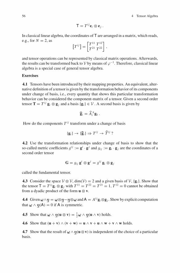
56 4 Tensor Algebra
T = T i jei ⊗ e j .
In classical linear algebra, the coordinates of T are arranged in a matrix, which reads,e.g., for N = 2, as
[
T i j] =
[
T 11 T 12
T 21 T 22
]
,
and tensor operations can be represented by classical matrix operations. Afterwards,the results can be transformed back to V by means of ϕ−1. Therefore, classical linearalgebra is a special case of general tensor algebra.
Exercises
4.1 Tensors have been introduced by their mapping properties. An equivalent, alter-native definition of a tensor is given by the transformation behavior of its componentsunder change of basis, i.e., every quantity that shows this particular transformationbehavior can be considered the component-matrix of a tensor. Given a second ordertensor T = T i j gi ⊗ g j and a basis {gi } ∈ V . A second basis is given by
gi = A ki gk .
How do the components T i j transform under a change of basis
{gi } → {gi } ⇒ T i j → T i j ?
4.2 Use the transformation relationships under change of basis to show that theso-called metric coefficients gi j := gi · g j and gi j := gi · g j are the coordinates of asecond order tensor
G = gi j gi ⊗ g j = gi j gi ⊗ g j
called the fundamental tensor.
4.3 Consider the space V ⊗ V , dim(V) = 2 and a given basis of V , {gi }. Show thatthe tensor T = T i jgi ⊗ g j with T 11 = T 22 = T 21 = 1, T 12 = 0 cannot be obtainedfrom a dyadic product of the form u ⊗ v.
4.4 Givenω˜
∧η˜
= ω˜
⊗η˜
−η˜
⊗ω˜
andA = Ai jgi⊗g j . Showby explicit computationthat ω
˜
∧ η˜
(A) = 0 if A is symmetric.
4.5 Show that ω˜
∧ η˜
(u ⊗ v) = 12ω˜
∧ η˜
(u ∧ v) holds.
4.6 Show that (u + v) ∧ (v + w) = u ∧ v + u ∧ w + v ∧ w holds.
4.7 Show that the result ofω˜
∧η˜
(u⊗v) is independent of the choice of a particularbasis.

4.10 Relation with Classical Linear Algebra 57
4.8 Given V = R3 with the standard basis {ei }. An area element can be represented
by a bi-vector AA = a ∧ b
with a,b ∈ V .1. Express A by means of coordinates and base vectors.2. Determine the coordinates A12, A13 and A23 related to the following representation
of A:A = A12e1 ∧ e2 + A13e1 ∧ e3 + A23e2 ∧ e3 ,
3. Give an interpretation of the coordinates A12, A13 and A23.
4.9 Show by means of (4.20) that the skew-symmetric projection defined by (4.19)corresponds to the tensor
P = 1
2[δkoδlp − δloδ
kp] g k ⊗ g l ⊗ g
˜
o ⊗ g˜
p .
References
1. Jänich K (2001) Vector analysis. Undergraduate texts in mathematics. Springer, New York2. LeeM (2002) Introduction to smoothmanifolds. Graduate texts inmathematics. Springer, Berlin

Chapter 5Affine Space and Euclidean Space
Abstract Affine and euclidean space are discussed primarily in view of their useas models for physical space. Affine mappings and coordinate charts generated bythem are examined. Furthermore, topological aspects are addressed.
5.1 Definitions and Basic Notions
As mentioned earlier, the general idea of a model for physical space is to endow aset of points X with a structure which allows us to encode certain physical concepts.It seems obvious to try the simplest case first, namely a point set X together with alinear structure. This, on the other hand, is tantamount to combining X with a vectorspace V . In addition, the model for space should allow for choosing an origin freely.Such a model is called affine space. It relies on the idea of assigning vectors to pairsof points by means of some mapping F . However, an affine structure on X requiresmore than just that, but such an assignment has to be consistent with the vector spaceoperations. In order to achieve this, F has to obey certain rules which form part ofthe following definition.
Definition 5.1 (Affine space) An affine space A = (X,V, F) consists of a point setX , a vector space V according to Definition3.1 and a mapping F ,
F : X × X → V(p, q) �→ F(p, q) = v ,
with the following properties for p0, p, r, q ∈ X and v ∈ V:(i) F(p, q) = −F(q, p)(ii) F(p, q) = F(p, r) + F(r, q)
(iii) For all p0 and v, there exists a unique q, such that F(p0, q) = v.
© Springer International Publishing AG 2017U. Mühlich, Fundamentals of Tensor Calculus for Engineers with a Primeron Smooth Manifolds, Solid Mechanics and Its Applications 230,DOI 10.1007/978-3-319-56264-3_5
59

60 5 Affine Space and Euclidean Space
Example 5.1 Points in R2 are represented by pairs of real numbers, e.g., the point pcorresponds to (p1, p2) with p1, p2 ∈ R. A mapping F is usually defined by
F(p, q) =[q1 − p1
q2 − p2
],
by which the point set R2 becomes an affine space.
The dimension of an affine space coincides with the dimension of the associatedvector space.One of themost important properties of an affine space is that everythingwhich can be interpreted as a result of F is an element of V and can, therefore,be added with any other element of V (see (ii) of Definition5.1). Furthermore, anaffine space is homogeneous and isotropic. The choice of a particular point p0 (seeDefinition5.1 (iii)) is equivalent to choosing an origin. After choosing an origin, anaffine space is indistinguishable from V .Example 5.2 Figure5.1 illustrates a possible exploration of space applying the affinespace concept. It sketches a bird’s eye view of a limited part of the surface of theearth. The filled polygons could be the roofs of houses. Some landmarks in termsof corners of these houses are chosen. One point, e.g., p0, is defined as origin. Pairsof points are chosen and respective vectors are assigned to these pairs by meansof a mapping F . The pairs (p0, p) and (p0, q) could be used to define a basisg1 = F(p0, p), g2 = F(p0, q). A point z can be addressed now by a correspondingvector z = F(p0, x), and z can be expressed by means of the base vectors andrespective coordinates
z = z1g1 + z2g2 .
g 1g 2
z
q
p
p0
z
F0 = F (p0, ♦)
XV
Fig. 5.1 Sketch regarding the exploration of the space of observation X based on the assumptionthat X is an affine space and choosing p0 as the origin. The symbol ♦ indicates a place-holder

5.1 Definitions and Basic Notions 61
The example illustrates the limits of this concept as well. The reader is encouragedto reflect on the situation described here in terms of the validity of the concept inrelation to the extension of the surface explored this way.
An affine space does not provide a structure which allows for measuring length,distance, or angles. A model for space, for which these concepts make sense, can bederived from an affine space in the following manner.
Definition 5.2 (Euclidean space E) An affine space where V is an inner productspace is an euclidean space.
5.2 Alternative Definition of an Affine Space by HybridAddition
Definition 5.3 (Hybrid addition of points and vectors) Given an affine space accord-ing to Definition5.1 with {V,⊕,�}. Hybrid addition “✛ ” is a mapping
✛ : X × V → X
(p,u) �→ q = p ✛ u
with the properties:
(i) [p ✛u] ✛ v = p ✛ [u ⊕ v](ii) p ✛ u = p implies u = 0(iii) For all p, q, there exists a unique u such that q = p ✛ u.
The properties of the hybrid addition can be deduced from the properties of F inDefinition5.1, and vice versa (see e.g., Epstein [2]). This means that hybrid additionand F are equivalent. Therefore, an affine space can be defined either by (X,V, F)
as in Definition5.1 or by (X,V, ✛ ).Hybrid addition is rather useful for encoding geometrical concepts transparently.
A straight line L , for instance, can simply be expressed by
L = p ✛ λu .
Furthermore, L is parallel with respect to another straight line L
L = q ✛ λv .
if u and v are linearly dependent. If, in addition, p = q, then L = L .

62 5 Affine Space and Euclidean Space
5.3 Affine Mappings, Coordinate Charts and TopologicalAspects
Within this section, mappings are discussed which preserve the affine structure. Twoaffine spaces A1 = (X1,V1, F1) and A2 = (X2,V2, F2) are considered. Due to thecorrespondence of X1 and V1 established by F1, respectively X2 and V2 due to F2,every affine mapping
μ : X1 → X2 ,
automatically induces a mapping A : V1 → V2, and vice versa. Furthermore, everylinear mapping between V1 and V2, as well as every global shift, preserves the affinestructure. This is the essence of the following definition.
Definition 5.4 (Affine mapping) Given two affine spaces (X1,V1, F1), (X2,V2, F2)
according to Definition5.1 and some linear mapping B : V1 → V2. A mapping μ :X1 → X2 with the property
B( F1(p, q) ) = F2(μ(p),μ(q) )
is called an affine mapping.
The most general form of μ which ensures that μ is an affine mapping accordingto Definition5.4 reads as
μ : X1 → X2
q �→ Q ✛B(F1(p0, q)) ,
where Q ∈ X2 and p0 ∈ X1 can be chosen arbitrarily. The second-order tensor Bencodes the mapping between the respective vector spaces.
Affine coordinate charts, also called affine coordinate systems, are common appli-cations of themappings discussed above. In the following,we consider an affine spaceA = (X,V, ✛ ). Explanations will be given by means of examples corresponding todim(A) = dim(V) = 2.
In X , there exist points, curves, e.g., Γ : R → X and functions, e.g.,Φ : A → R.In order to be able to perform computations with numbers, a pair of real numbers isassigned to each point by a mapping
μ : X → R2
p �→ (x1(p), x2(p)) ,
where xi (p) : A → R is called the i-th coordinate function because it assigns to apoint p its i-th coordinate. The mapping μ generates a coordinate system, also calleda coordinate chart. Different mappings of this kind establish different coordinatesystems. As illustrated in Fig. 5.2, these systems differ in the meaning of a specific

5.3 Affine Mappings, Coordinate Charts and Topological Aspects 63
p
q
µ(p)
µ(q)
µ(p)
µ(q)
Γ
X R2
R
Fig. 5.2 Sketch illustrating the effect of two affine mappings μ and μ on two points p and q,respectively, on a curve in X
p
q
µ(p)
µ(q)
µ(p)
µ(q)
Γ
X
R2
R2
R
µ µ
µ ◦ µ−1
Fig. 5.3 Visualization of different coordinate charts established by different mappings and thetransition between these charts
pair of real numbers. However, the visualization in Fig. 5.2 will become confusingas the complexity of the problem increases.
Therefore, a different visualization is commonly preferred which better accountsfor the transition between different coordinate charts. This is illustrated in Fig. 5.3.

64 5 Affine Space and Euclidean Space
When referring to coordinate charts of A established by mappings μ and μ, thenotations (X,μ) and (X, μ) are used in the following. In order to distinguish betweenthe function Φ and its representation in a chart f = Φ ◦ μ−1, the notation
f = f (x1, x2) (5.1)
with f = Φ ◦ μ−1 is employed in general, which reveals a common notational abuse(see e.g., Crampin and Pirani [1]), since in (5.1), the xi are coordinates and notcoordinate functions. Hence, (x1, x2) denotes either a point in R
2, the coordinatesof a point in X , or the mappings which generate the coordinate system (X,μ).Although the specific meaning of xi is usually clear from the context, it requires acareful reading of the respective equations in order to avoid misinterpretations andmistakes. Similarly,
f = f (x1, x2)
expresses that f = Φ ◦ μ−1 is the coordinate representation of Φ in chart (A, μ).The transition between (A,μ) and (A, μ) is expressed by the mapping
g = μ ◦ μ−1 : R2 → R2
(x1, x2) �→ (x1(x1, x2), x1(x1, x2)) ,
where the x i are actually again coordinate functions, whereas the xi are coordinatesof points in R2.
In the following, we consider Example 5.2 together with a mapping from V intothe R2, which just reads off the coordinates of z related to the basis {gi }
ϕ : V → R2 (5.2)
z = z1g1 + z2g2 �→ (x1 = z1, x2 = z2) .
Its inverse is given by
ϕ−1 : R2 → V(z1, z2) �→ z = z1g1 + z2g2 .
A topology can be defined for V by the collection of all sets U of the standardtopology of R2 under ϕ−1, i.e., ϕ−1(U ). Obviously, ϕ and ϕ−1 are continuous forthis topology, and since ϕ is a homeomorphism, φ = ϕ ◦ F , is a coordinate chart,according to Definition2.12.
The generalization for arbitrary but finite dimensions is straightforward. Since Vcan be endowed with a topology, an affine space is a possible model for physicalspace, but again, it depends on the problem as to whether it is also a suitable model.
The compositionμ = ϕ ◦ F sketched in Fig. 5.4 is an affinemappingμ : X → R2
according to Definition5.4 with Q = (0, 0) and

5.3 Affine Mappings, Coordinate Charts and Topological Aspects 65
g 1
g 2
g 1
g 2
e1e1
e2e2
p0p1
p2
q1
q2
µ µ
µ ◦ µ−1
ΓR
µ(p0) µ(p1)
µ(p2)
µ(q1)
µ(q2)
µ(p0)
µ(q1)
µ(q2)
µ(p1)
µ(p1)
X
V
R2
R2
Fig. 5.4 Sketch of the affine coordinates which result from the mappings μ and μ, where thesemappings differ with respect to the choice of base vectors in V and {e1, e2} is the standard basisin R
2
B = δikei ⊗ g˜k , (5.3)
where {ei } is the standard basis in R2. This is an example for a basis isomorphism.A second mapping μ using a different origin p0 and a basis
{gi
}is considered.
While a point x ∈ X has coordinates (x1, x2) in the chart induced by μ, the samepoint is referred to by the coordinates (x1, x2) in the chart induced by μ. In order tofigure out how these coordinates are related, (iii) of Definition5.1 is applied:
F(p0, x) = F(p0, p0) + F( p0, x) , (5.4)
where the LHS corresponds to x, the term F( p0, x) equals x and F(p0, p0) is ashift due to the change of the origin called c in the following. According to thetransformation rules given in Box3.4.1, the base vectors gi and g j are related by
gi = A ki gk .
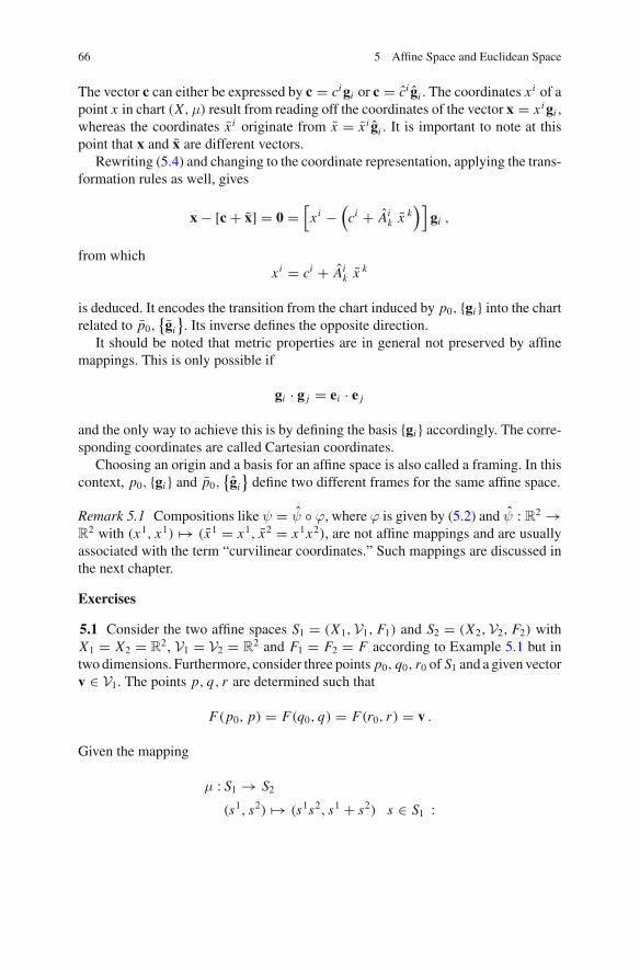
66 5 Affine Space and Euclidean Space
The vector c can either be expressed by c = cigi or c = ci gi . The coordinates xi of a
point x in chart (X,μ) result from reading off the coordinates of the vector x = xigi ,whereas the coordinates x i originate from x = x i gi . It is important to note at thispoint that x and x are different vectors.
Rewriting (5.4) and changing to the coordinate representation, applying the trans-formation rules as well, gives
x − [c + x] = 0 =[xi −
(ci + Ai
k xk)]
gi ,
from whichxi = ci + Ai
k xk
is deduced. It encodes the transition from the chart induced by p0, {gi } into the chartrelated to p0,
{gi
}. Its inverse defines the opposite direction.
It should be noted that metric properties are in general not preserved by affinemappings. This is only possible if
gi · g j = ei · e j
and the only way to achieve this is by defining the basis {gi } accordingly. The corre-sponding coordinates are called Cartesian coordinates.
Choosing an origin and a basis for an affine space is also called a framing. In thiscontext, p0, {gi } and p0,
{gi
}define two different frames for the same affine space.
Remark 5.1 Compositions like ψ = ψ ◦ ϕ, where ϕ is given by (5.2) and ψ : R2 →R
2 with (x1, x1) �→ (x1 = x1, x2 = x1x2), are not affine mappings and are usuallyassociated with the term “curvilinear coordinates.” Such mappings are discussed inthe next chapter.
Exercises
5.1 Consider the two affine spaces S1 = (X1,V1, F1) and S2 = (X2,V2, F2) withX1 = X2 = R
2, V1 = V2 = R2 and F1 = F2 = F according to Example 5.1 but in
two dimensions. Furthermore, consider three points p0, q0, r0 of S1 and a given vectorv ∈ V1. The points p, q, r are determined such that
F(p0, p) = F(q0, q) = F(r0, r) = v .
Given the mapping
μ : S1 → S2
(s1, s2) �→ (s1s2, s1 + s2) s ∈ S1 :

5.3 Affine Mappings, Coordinate Charts and Topological Aspects 67
(a) Determine the images of the points p0, p, q0, q, r0, r in S2 under μ.(b) Determine the vectors
a = F(μ(P0),μ(P)) , b = F(μ(Q0),μ(Q)) , c = F(μ(R0),μ(R)) ,
where a,b, c ∈ V2.(c) The vector spaces V1 and V2 can be related by a linear mapping which is an
isomorphism (1-1 and onto), but is there a unique mapping which maps a,b, c ∈V∈ to v ∈ V1?
5.2 Perform Exercise5.1 for
μ : S1 → S2
(s1, s2) �→ (s1 + s2, s1 − s2) s ∈ S1 .
References
1. Crampin M, Pirani F (1987) Applicable differential geometry, vol 58. London mathematicalsociety lecture note series. Cambridge University Press, Cambridge
2. Epstein M (2010) The geometrical language of continuum mechanics. Cambridge UniversityPress, Cambridge

Chapter 6Tensor Analysis in Euclidean Space
Abstract After briefly reviewing differentiability in R, a generalization of differ-entiability based on the directional derivative in R
N is established. Gradients ofscalar and vector fields are first discussed in R
N before adapting these concepts forgeneral euclidean spaces in combination with global charts. Afterwards, nonlinearchart relations, also known as curvilinear coordinates, are examined, and the conceptof tangent space at a point is introduced. In this context, the covariant derivativeis derived, insinuating its character as special case of the covariant derivative forsmooth manifolds. Aspects of integration based on differential forms are discussedtogether with the exterior derivative and Stoke’s theorem in R
N .
6.1 Differentiability inRRR and Related ConceptsBriefly Revised
The derivative from the left of a function f (x) at some x = x0 is defined by
d f
dx
∣∣∣∣x0−
= limh→0−
1
h[ f (x0 + h) − f (x0)] , (6.1)
whereas the derivative from the right may be written as
d f
dx
∣∣∣∣x0+
= limh→0+
1
h[ f (x0 + h) − f (x0)] . (6.2)
These derivatives may or may not exist. If they exist, they may be equal or not. Theexistence and equality of both derivatives is referred to as a continuous derivative. Itimplies continuity of f at x = x0 and
d f
dx
∣∣∣∣x0
= limh→0
1
h[ f (x0 + h) − f (x0)] (6.3)
© Springer International Publishing AG 2017U. Mühlich, Fundamentals of Tensor Calculus for Engineers with a Primeron Smooth Manifolds, Solid Mechanics and Its Applications 230,DOI 10.1007/978-3-319-56264-3_6
69

70 6 Tensor Analysis in Euclidean Space
is sufficiently precise. The reverse does not hold, a fact that can be seen easily fromthe standard example f (x) = |x |, which is continuous at x = 0 but not continuouslydifferentiable. The derivative at some arbitrary x is indicated by d f
dx , and performingthis operation yields a function of x . That way, derivatives of arbitrary order can bedefined for which the notation
dk f
dxk
∣∣∣∣x0
= limh→0
1
h
[dk−1
dxk−1f (x0 + h) − dk−1
dxk−1f (x0)
]
k = 1, . . . , N
is commonly employed together with the definition
d0
dx0f := f .
This allows for a classification of functions by the following definition.
Definition 6.1 (Set of continuously differentiable functions) The set of all functionsdefined on an interval [a, b] or [a, b), etc., having continuous derivatives up to orderk is called Ck([a, b]), or Ck([a, b)), respectively, etc. If the interval is (−∞,+∞),the notation Ck(R) is used.
The scheme sketched so far is rather intuitive and successful. However, it is notobvious how we might transfer the concept of being continuously differentiable ina straightforward manner to higher dimensions, and more general objects, such astensor fields over RN . In order to obtain hints as to what a more general schememight look like, it is useful to dissect (6.3) first. If f is continuously differentiableat x0, then (6.3) exists and can be written as
limh→0
1
h
[
f (x0 + h) − f (x0) − d f
dx
∣∣∣∣x0
h
]
= 0 . (6.4)
It reveals that being continuously differentiable implies the existence of a uniquelinear approximation of f at x0,
d|x0 f (h) = d f
dx
∣∣∣∣x0
h , (6.5)
which is the differential of f at x0 and usually denoted by d f |x0 . The reason foremploying a more expressive notation will become clear shortly. If f is continuouslydifferentiable at x0, then the differential is unique, because in this case, there exists,
by definition, exactly one number d fdx
∣∣∣x0. In one dimension, this also implies linearity
of (6.5). The differential (6.5) can also be written as
dh |x0 f = limt→0
1
t[ f (x0 + th) − f (x0)] , (6.6)

6.1 Differentiability in R and Related Concepts Briefly Revised 71
which is the so-called directional derivative in one dimension. It has a straightfor-ward generalization to higher dimensions just by replacing x0 + th by, e.g., p0 ✛ th.Furthermore, general tensor functions on RN , e.g., A(p), do not induce any concep-tual difficulty either. However, (6.6) must be handled with care, since it can also becomputed for functions which are not continuously differentiable (see Exercise 6.2).The key is that continuous differentiability not only implies the existence of (6.6),but also its linearity wrt. h, or—vice versa—the existence of (6.6) implies contin-uous differentiability only if (6.6) is also linear wrt. h. Hence, the following threestatements are equivalent:
1. the function f (x) is continuously differentiable at x = x0,2. the derivatives (6.1) and (6.2) exist and are equal,3. there exists a unique linear approximation of f (x) at x = x0,
where the second statement is tantamount to (6.3).In the following, only functions belonging to C∞ are considered in order to keep
the discussion simple. Then, the right hand side of (6.6) can be interpreted as a linearmapping from C∞ into R,
dh |x0 : C∞(R) → R
or as a linear mapping from R into R
d|x0 f : R → R ,
depending on whether a function f or a real number h is considered as the argumentof (6.6).
If a function f is differentiable at a certain x = x0, it can be approximated by aTaylor series
f (x0 + t) ≈ f (x0) + d f
dx
∣∣∣∣x0
t + 1
2
d2 f
dx2
∣∣∣∣x0
t2 + · · ·
in the vicinity of x0 exclusively using information about f at x0.In what follows, we consider a function f (x) together with a mapping
g : R → R
x �→ y = α(x) ,
where α is a function of x , e.g., α = 2x . By means of its inverse
g−1 : R → R
y �→ x = β(y)

72 6 Tensor Analysis in Euclidean Space
the functionΦ = f ◦ g−1 = f (β(y))
can be defined. With a slight abuse of notation, Φ(y) = f (x(y)) is commonly used,as long as it does not cause confusion. The derivative ofΦ with respect to y at y = y0reads as
dΦ
dy
∣∣∣∣y0
= limt→0
1
t[Φ(y0 + t) − Φ(y0)]
= limt→0
1
t[ f (x(y0 + t)) − f (x(y0))] . (6.7)
Linearizing first x(y0 + t) by applying Taylor series expansion
x(y0 + t) ≈ x(y0) + dx
dy
∣∣∣∣y0
t
and taking into account that x(y0) = x0, a subsequent linearization can be performed:
f (x(y0 + t)) ≈ f (x0) + d f
dx
∣∣∣∣x0
dx
dy
∣∣∣∣y0
t . (6.8)
Using (6.8), (6.7) finally gives
dΦ
dy
∣∣∣∣y0
= d f
dx
∣∣∣∣x0
dx
dy
∣∣∣∣y0
(6.9)
which is known as chain rule in R.
6.2 Generalization of the Concept of Differentiability
Apowerful generalization of (6.6) is provided by the so-called directional derivative.
Definition 6.2 (Directional derivative) Given some finite-dimensional euclideanspace En = (X,V, ✛ ) and a mapping F : U → V where U is an open subset ofX and V is some vector space. The directional derivative of F at point p in thedirection determined by h ∈ V is defined by
d˜
|p F(h) = limt→0
1
t[F(p ✛ th) − F(p)] .
Because Definition 6.2 refers to the difference of images ofF ,V has to be a vectorspace. Since the limit is performed with respect to a real number, Definition 6.2 is

6.2 Generalization of the Concept of Differentiability 73
extremely flexible in terms ofF . Possible examples forF areF : U → R,F : U →W or F : U → W ⊗ W , etc., and V and W do not have to be equal. The directionalderivative forms part of the following definition of differentiability.
Definition 6.3 (Differentiability in En) Given some finite dimensional euclideanspace En = (X,V, ✛ ) and a mapping F : U → V where U is an open subset of Xand V is some vector space. F is differentiable at p if
limh→0
1
||h||[
F(p ✛ h) − F(p) − d˜
|p F(h)]
= 0
exists, and in addition, d|p F(h) is linear wrt. h ∈ V .Definition 6.3 is based on the idea of relating differentiability to the existence of
a linear approximation, as discussed within the previous section. It is worth notingthat Definition 6.3 relies only on the norm defined for En . Of course, the meaning ofthe RHS in Definition 6.3 depends on the meaning of F .
It can be shown that if the directional derivative of F is linear with respect to h,then F is differentiable in the sense of Definition 6.3. The type of linear mappingwhich ensures differentiability ofF under consideration can be read off immediatelyfrom Definition 6.3. This allows for computing the linear approximation at a specificpoint and is discussed in the following.
It should be noted that Definitions 6.2 and 6.3 are also known as the Gateauxdifferential and the Fréchet derivative, respectively, in the much wider context offunctional analysis in Banach spaces. Without going into detail, we remark thatfinite dimensional euclidean spaces are Banach spaces. However, the latter havebeen designed in the first place for infinite dimensional vector spaces, e.g., the spaceof all functions of a certain type defined on the interval [a, b] ⊂ R.
Functions were characterized in Sect. 1.4 as mappings which assign a real numberto every point of a given set. On the other hand, functions are also called scalar fields.Consistently, mappings which assign a vector to every point of a set are also knownas vector fields. In the following, these terms are also used, because the term tensorfield is simpler than talking about a mapping which assigns a tensor to every point.
6.3 Gradient of a Scalar Field and Related Concepts inRRRN
In RN , every point is addressed by an N-tuple of real numbers (see Definition 3.8).
As already pointed out in Sect. 4.10, the standard basis {ei } in RN corresponds to
columns with N entries. The k th base vector ek consists of zeros, except for the k th
entry, which equals one.For R
N endowed with the usual inner product,⟨
e˜
i , e j⟩ = ei · e j holds (see
Sect. 3.8). This allows for replacing dual vectors with reciprocal vectors, and cor-respondingly dual products with inner products. Here, we will make use of this

74 6 Tensor Analysis in Euclidean Space
eventually in order to provide those operators commonly used in conventional vec-tor analysis.
Since {ei } is an orthonormal basis, base vectors and reciprocal base vectors evencoincide, i.e., ei = ei . Therefore, provided that summation convention is adaptedaccordingly, the distinction between vectors and reciprocal vectors, and correspond-ingly lower and upper indices, could be dropped as well. However, this implies theabandonment of a simple and efficient control mechanism regarding index notation.More importantly, all underlying structure becomes invisible without any real benefitin return. Therefore, we continue with the notation used so far.
For a given scalar function f : RN → R to be continuously differentiable,d |p F(h) in (6.3) has to be a linear mapping
d |p f : V → R , (6.10)
with V = RN . Please note the subtlety in the meaning ofRN . While in the definition
of f ,RN means just the set of points, (6.10) refers toRN as a vector space accordingto Definition 3.8. Linearity is explored by applying the very same chain of stepswidely used in Chap.4,
d |p f (h) = hi d˜
∣∣p f (ei ) , (6.11)
where the d˜
∣∣p f (ei ) have to be real numbers. The abbreviation
λi := d˜
∣∣p f (ei )
is used in the following. The remaining steps aim to separate the objectwhich encodesthe mapping (6.10) from the argument. This yields
d |p f (h) = hiλi = λi⟨
e˜
i ,h⟩ = λi e
˜
i (h) ,
and therefored |p f = λi e
˜
i . (6.12)
This is the so-called gradient of f at p, which is a dual vector, i.e., d |p f ∈ V∗.Computation of the coordinates λi requires the notion of partial derivatives.
Definition 6.4 (Partial derivatives in RN ) The partial derivatives of a function
f (x1, x2, . . . , xN ) at a point p = (p1, p2, . . . , pN ) with respect to the coordinatexk , where k = 1 . . . N , are defined by
∂ f
∂xk
∣∣∣∣p−
= limt→0−
1
t
[
f (p1, . . . , pk−1, pk + t, pk+1, . . . , pN ) − f (p1, p2, . . . , pN )]
∂ f
∂xk
∣∣∣∣p+
= limt→0+
1
t
[
f (p1, . . . , pk−1, pk + t, pk+1, . . . , pN ) − f (p1, p2, . . . , pN )]
,

6.3 Gradient of a Scalar Field and Related Concepts in RN 75
and if both derivatives exist and are equal,
∂ f
∂xk
∣∣∣∣p
= limt→0
1
t
[
f (p1, . . . , pk−1, pk + t, pk+1, . . . , pN ) − f (p1, p2, . . . , pN )]
is used.
For the sake of simplicity, we first consider the case N = 2 in (6.10). Accordingto Definition 6.4, there are two partial derivatives in R2:
∂ f
∂x1
∣∣∣∣p
= limt→0
1
t
[
f (p1 + t, p2) − f (p1, p2)]
∂ f
∂x2
∣∣∣∣p
= limt→0
1
t
[
f (p1, p2 + t) − f (p1, p2)]
.
Comparing Definition 6.4 with Eq. 6.11, taking into account hybrid addition in R2,
reveals that∂ f
∂x1
∣∣∣∣p
= d |p f (e1) ,∂ f
∂x2
∣∣∣∣p
= d |p f (e2) ,
since p ✛ te1 = (p1, p2) ✛ t
(
10
)
= (p1 + t, p2), and similarly for p ✛ te2. This
extends to higher dimensions, i.e.,
∂ f
∂xi
∣∣∣∣p
= d |p f (ei ) . (6.13)
On the other hand,d |p f (ei ) = λk
⟨
e˜
k, ei⟩ = λi , (6.14)
and therefore
d |p f = ∂ f
∂xi
∣∣∣∣p
e˜
i (6.15)
results. Furthermore, (6.15) shows that inRN , Definition 6.3 is equivalent to the exis-tence of partial derivatives. Therefore, an alternative definition of being continuouslydifferentiable can be given.
Definition 6.5 (Set of continuously differentiable functions in RN ) The set of all
functions defined on RN having continuous partial derivatives up to order k is calledCk(RN ).
Not only are scalar fields usually of interest, but vector fields are as well. Next,we consider a vector field
f : RN → W
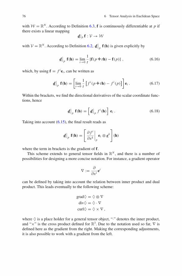
76 6 Tensor Analysis in Euclidean Space
with W = RN . According to Definition 6.3, f is continuously differentiable at p if
there exists a linear mappingd |p f : V → W
with V = RN . According to Definition 6.2, d
˜
∣∣p f(h) is given explicitly by
d˜
∣∣p f(h) = lim
t→0
1
t[f(p ✛ th) − f(p)] , (6.16)
which, by using f = f iei , can be written as
d˜
∣∣p f(h) =
[
limt→0
1
t
[
f i (p ✛ th) − f i (p)]]
ei . (6.17)
Within the brackets, we find the directional derivatives of the scalar coordinate func-tions, hence
d˜
∣∣p f(h) =
[
d˜
∣∣p f i (h)
]
ei . (6.18)
Taking into account (6.15), the final result reads as
d˜
∣∣p f(h) =
[
∂ f i
∂xk
∣∣∣∣p
ei ⊗ e˜
k
]
(h)
where the term in brackets is the gradient of f .This scheme extends to general tensor fields in R
N , and there is a number ofpossibilities for designing a more concise notation. For instance, a gradient operator
∇ := ∂
∂xiei
can be defined by taking into account the relation between inner product and dualproduct. This leads eventually to the following scheme:
grad♦ = ♦ ⊗ ∇div♦ = ♦ · ∇curl♦ = ♦ × ∇ ,
where ♦ is a place holder for a general tensor object, “·” denotes the inner product,and “×” is the cross product defined for R3. Due to the notation used so far, ∇ isdefined here as the gradient from the right. Making the corresponding adjustments,it is also possible to work with a gradient from the left.

6.4 Differentiability in Euclidean Space Supposing Affine Relations 77
6.4 Differentiability in Euclidean Space SupposingAffine Relations
Analysis inRN usuallymeans treating some real world problem employing an appro-priate coordinate chart. In what follows, the aim is to discuss how to relate analysisregarding physical space with the results obtained within the previous section, pro-vided all involved mappings between charts and physical space are affine mappings.Such charts are called affine charts in the following.
For a given scalar field Φ defined over an euclidean space E = (X,V, ✛ ) andcontinuously differentiable at point p, d
˜
∣∣p F(h) in (6.3) has to be a linear mapping
d˜
∣∣p Φ : V → R . (6.19)
By now it should be clear that d˜
∣∣p Φ ∈ V∗ (see Sect. 3.6). Choosing a basis {gi } for
V and exploring linearity again eventually yields
d˜
∣∣p
Φ = Li g˜
i . (6.20)
However, this result is only useful if the coordinates Li of L˜
can be computed.Computation, on the other hand, requires a chart. Since affine mappings are globalhomeomorphisms, i.e., they are invertible everywhere, we can work with globalcharts as long as the latter are generated by affine mappings. We consider a chart(X,μ) induced by a mapping μ : X → R
N . The image of Φ in the chart is given byf = Φ ◦ μ−1, and regarding the corresponding d |μ(p) f , we just have to adapt (6.15)accordingly
d˜
∣∣μ(p) f = ∂ f
∂xi
∣∣∣∣μ(p)
e˜
i ,
where μ(p) is the image of p in the chart. This is sketched for a two-dimensionalproblem in Fig. 6.1.
The value of Φ at a point p coincides with the value of f at the image of p inthe chart, i.e., Φ(p) = f (μ(p)). The operation d
˜
∣∣p Φ(H) refers to a limit process
passing through points in X addressed by p ✛ tH. If the limit process in the chart,d˜
∣∣μ(p) f (h), passes through the images of the very same points, then both limit
processes yield identical results.Sinceμ is an affinemapping according to Definition 5.4 with an associated second
order tensor B, then μ(q) = μ(p) ✛B(V) holds for two points p and q in X relatedby q = p ✛V. Therefore,
d˜
∣∣p Φ(H) = d
˜
∣∣μ(p) f (h ) (6.21)
holds if h = B(H). The tensor B encodes a mapping

78 6 Tensor Analysis in Euclidean Space
x1
x2
x 1
x 2
p
q
μ(p)
μ(q)
μ(p)
μ(q)
g
g−1
A
μ μ
e1
e2
e1
e2
h
h
H
Φ
f = Φ ◦ μ−1f = Φ ◦ μ−1
V
Fig. 6.1 Contour plot of a function Φ in a two-dimensional euclidean spaces together with twopossible charts induced by affine mappings
μ� : V → RN (6.22)
called the push forward under the mapping μ. It relates the two vector spaces V andR
N based on (6.21), i.e., it establishes a correspondence between H and h in thesense that H acts on Φ as h acts on the image of Φ in the chart induced by μ. Itsdual, defined by (see Sect. 4.3)
⟨
μ�(η˜
),H⟩
=⟨
η˜
,μ�(H)⟩
, (6.23)
relates the corresponding dual spaces
μ� : RN∗ → V∗ (6.24)

6.4 Differentiability in Euclidean Space Supposing Affine Relations 79
and is called the pull back under μ. The reason for assigning specific names to themappings (6.22) and (6.24) lies in the importance of the underlying concepts. Thisis discussed in more detail later.
Evaluating (6.21) for the corresponding bases and taking into account the corre-spondence between h and H gives
LkHk = ∂ f
∂xi
∣∣∣∣μ(p)
hi = ∂ f
∂xi
∣∣∣∣μ(p)
Bik H
k , (6.25)
from which
d˜
∣∣pΦ = ∂ f
∂xi
∣∣∣∣μ(p)
Bik g˜
k = ∂ f
∂xi
∣∣∣∣μ(p)
e˜
i (6.26)
follows. Depending on which coordinate base vector representation for the gradientof Φ is used, the corresponding argument, either H = Hkgk or h = hkek , has to beprovided when computing the directional derivative.
In the particularly simple case of affine coordinates, Bik = δik holds and, therefore,
d˜
∣∣pΦ = ∂ f
∂xi
∣∣∣∣μ(p)
g˜
i = ∂ f
∂xi
∣∣∣∣μ(p)
e˜
k ,
which means that, at first glance, there is no difference to analysis in RN except for
the fact that f means the image of some function Φ. But for transferring resultsobtained through computations performed in charts back into the real world, the wayphysical space has been explored must be taken into account, i.e., eventually themeaning of the gi matters.
In order to check that the scheme discussed above does not depend on the choicefor a chart, another affine mapping μ with its associated second order tensor B isconsidered. It induces a chart (X,μ) ⊂ R
N with coordinates x k , and the image of Φ
in this chart is f = Φ ◦ μ−1. Analogously to the case discussed above, we demand
d˜
∣∣p Φ(H) = d
˜
∣∣μ(p) f (h ) , (6.27)
which is fulfilled if h = B(H).The aim in what follows is to show that the result for d
˜
∣∣p
Φ(H) does not dependon the choice for a particular chart by showing that the right hand sides of (6.21) and(6.27) coincide, i.e.,
d˜
∣∣μ(p)
f (h ) = d˜
∣∣μ(p)
f (h ) .
This requires some preparatory work. Using the identity
Φ ◦ μ−1 = Φ ◦ μ−1 ◦ μ ◦ μ−1 , (6.28)
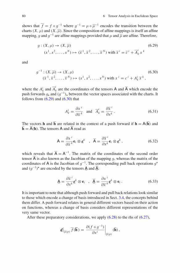
80 6 Tensor Analysis in Euclidean Space
shows that f = f ◦ g−1 where g−1 = μ ◦ μ−1 encodes the transition between thecharts (X,μ) and (X,μ). Since the composition of affine mappings is itself an affinemapping, g and g−1 are affine mappings provided that μ and μ are affine. Therefore,
g : (X,μ) → (X,μ) (6.29)
(x1, x2, . . . , xN ) �→ (x 1, x 2, . . . , x N ) with x i = c i + Aik x
k
and
g−1 : (X,μ) → (X,μ) (6.30)
(x 1, x 2, . . . , x N ) �→ (x1, x2, . . . , xN ) with x i = c i + Aik x
k ,
where the Aik and A
ik are the coordinates of the tensors A and A which encode the
push forwards g� and (g−1)� between the vector spaces associated with the charts. Itfollows from (6.29) and (6.30) that
Aik = ∂x i
∂x k and Aik = ∂x i
∂xk. (6.31)
The vectors h and h are related in the context of a push forward if h = A(h) andh = A(h). The tensors A and A read as
A = ∂x i
∂x k ei ⊗ e˜
k , A = ∂x i
∂xkei ⊗ e
˜
k , (6.32)
which reveals that A = A−1. The matrix of the coordinates of the second ordertensor A is also known as the Jacobian of the mapping g, whereas the matrix of thecoordinates of A is the Jacobian of g−1. The corresponding pull back operations g�
and (g−1)� are encoded by the tensors A˜and A
˜:
A˜
= ∂x i
∂xke˜
k ⊗ ei , A˜
= ∂x i
∂x k e˜
k ⊗ ei . (6.33)
It is important to note that although push forward and pull back relations look similarto those which encode a change of basis introduced in Sect. 3.4, the concepts behindthem differ. A push forward relates in general different vectors based on their actionon functions, whereas a change of basis considers different representations of thevery same vector.
After these preparatory considerations, we apply (6.28) to the rhs of (6.27),
d˜
∣∣μ(p) f (h ) = ∂( f ◦ g−1)
∂xi
∣∣∣∣μ(p)
(h) ,

6.4 Differentiability in Euclidean Space Supposing Affine Relations 81
which shows that a generalization of the chain rule (6.9) is needed to proceed. Thisgeneralization is not really challenging and is left as an exercise (see Exercise 6.4).Applying chain rule, also taking into account h = A(h), gives
d˜
∣∣μ(p) f (h ) = ∂ f
∂xi
∣∣∣∣μ(p)
∂xi
∂xk∂xk
∂xmhm = ∂ f
∂xi
∣∣∣∣∣μ(p)
h i ,
which reveals that (6.20) does not depend on the choice of a particular chart.
The directional derivative of a function defined in an N -dimensional euclideanspace E = (X,V, ✛ ) can be computed by using a chart (X,μ) ⊂ R
N obtainedfrom an affine mapping μ : X → R
N .
Similarly, the directional derivative d˜
∣∣p F(h) in (6.3) for a vector fieldW defined
over an euclidean space E = (X,V, ✛ ) is a linear mapping
d˜
∣∣p W : V → V
ifW is continuously differentiable. Adapting (6.16) and (6.17) accordingly yields
d˜
∣∣p W(H) =
[
d˜
∣∣p W
i (H)]
gi
for a basis {gi } ∈ V . After choosing a chart (X,μ)with μ according to Definition 5.4,(6.18) can be evaluated at a point p ∈ X by
d˜
∣∣p W(H) = ∂ wi
∂xk
∣∣∣∣μ(p)
BkmH
m gi
withwi = Wi ◦ μ−1. Separation of the mapping from the argument can be achieved,
as usual, by using Hm =⟨
g˜
m,H⟩
:
d˜
∣∣p W(H) =
[
∂ wi
∂xk
∣∣∣∣μ(p)
Bkm gi ⊗ g
˜
m
]
(H) ,
where the term within brackets is the gradient ofW at p with reference to the bases{gi } ∈ V . Using affine coordinates, the gradient of W reads as
d˜
∣∣p W = ∂ wi
∂xk
∣∣∣∣μ(p)
gi ⊗ g˜
k = ∂ wi
∂xk
∣∣∣∣μ(p)
ei ⊗ e˜
k ,
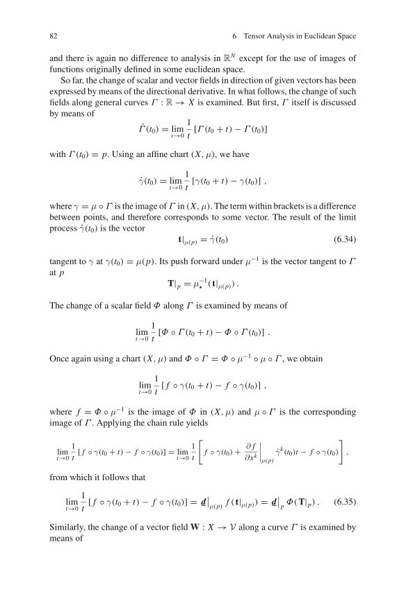
82 6 Tensor Analysis in Euclidean Space
and there is again no difference to analysis in RN except for the use of images of
functions originally defined in some euclidean space.So far, the change of scalar and vector fields in direction of given vectors has been
expressed by means of the directional derivative. In what follows, the change of suchfields along general curves Γ : R → X is examined. But first, Γ itself is discussedby means of
Γ (t0) = limt→0
1
t[Γ (t0 + t) − Γ (t0)]
with Γ (t0) = p. Using an affine chart (X,μ), we have
γ(t0) = limt→0
1
t[γ(t0 + t) − γ(t0)] ,
where γ = μ ◦ Γ is the image ofΓ in (X,μ). The termwithin brackets is a differencebetween points, and therefore corresponds to some vector. The result of the limitprocess γ(t0) is the vector
t|μ(p) = γ(t0) (6.34)
tangent to γ at γ(t0) = μ(p). Its push forward under μ−1 is the vector tangent to Γ
at pT|p = μ−1
� ( t|μ(p)) .
The change of a scalar field Φ along Γ is examined by means of
limt→0
1
t[Φ ◦ Γ (t0 + t) − Φ ◦ Γ (t0)] .
Once again using a chart (X,μ) and Φ ◦ Γ = Φ ◦ μ−1 ◦ μ ◦ Γ , we obtain
limt→0
1
t[ f ◦ γ(t0 + t) − f ◦ γ(t0)] ,
where f = Φ ◦ μ−1 is the image of Φ in (X,μ) and μ ◦ Γ is the correspondingimage of Γ . Applying the chain rule yields
limt→0
1
t[ f ◦ γ(t0 + t) − f ◦ γ(t0)] = lim
t→0
1
t
[
f ◦ γ(t0) + ∂ f
∂xk
∣∣∣∣μ(p)
γk(t0)t − f ◦ γ(t0)
]
,
from which it follows that
limt→0
1
t[ f ◦ γ(t0 + t) − f ◦ γ(t0)] = d
˜
∣∣μ(p) f ( t|μ(p)) = d
˜
∣∣p Φ(T|p) . (6.35)
Similarly, the change of a vector field W : X → V along a curve Γ is examined bymeans of
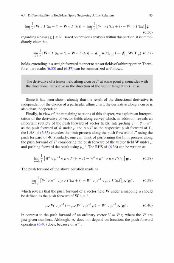
6.4 Differentiability in Euclidean Space Supposing Affine Relations 83
limt→0
1
t[W ◦ Γ (t0 + t) − W ◦ Γ (t0)] = lim
t→0
1
t
[
Wi ◦ Γ (t0 + t) − Wi ◦ Γ (t0)]
gi(6.36)
regarding a basis {gi } ∈ V . Based on previous analysis within this section, it is imme-diately clear that
limt→0
1
t[W ◦ Γ (t0 + t) − W ◦ Γ (t0)] = d
˜
∣∣p w( t|μ(p)) = d
˜
∣∣p W(T|p) (6.37)
holds, extending in a straightforwardmanner to tensor fields of arbitrary order. There-fore, the results (6.35) and (6.37) can be summarized as follows.
The derivative of a tensor field along a curve Γ at some point p coincides withthe directional derivative in the direction of the vector tangent to Γ at p.
Since it has been shown already that the result of the directional derivative isindependent of the choice of a particular affine chart, the derivative along a curve isalso chart independent.
Finally, in view of the remaining sections of this chapter, we explore an interpre-tation of the derivative of vector fields along curves which, in addition, reveals animportant subtlety of the push forward of vector fields. Interpreting f = Φ ◦ μ−1
as the push forward of Φ under μ and μ ◦ Γ as the respective push forward of Γ ,the LHS of (6.35) encodes the limit process along the push forward of Γ using thepush forward of Φ. Similarly, one can think of performing the limit process alongthe push forward of Γ considering the push forward of the vector field W under μand pushing forward the result using μ−1
� . The RHS of (6.36) can be written as
limt→0
1
t
[
Wi ◦ μ−1 ◦ μ ◦ Γ (t0 + t) − Wi ◦ μ−1 ◦ μ ◦ Γ (t0)]
gi . (6.38)
The push forward of the above equation reads as
limt→0
1
t
[
Wi ◦ μ−1 ◦ μ ◦ Γ (t0 + t) − Wi ◦ μ−1 ◦ μ ◦ Γ (t0)]
μ�(gi ) , (6.39)
which reveals that the push forward of a vector field W under a mapping μ shouldbe defined as the push forward ofW ◦ μ−1,
μ�(W ◦ μ−1) = μ�(Wi ◦ μ−1gi ) = Wi ◦ μ−1μ�(gi ) , (6.40)
in contrast to the push forward of an ordinary vector V = V igi where the V i arejust given numbers. Although, μ� does not depend on location, the push forwardoperation (6.40) does, because of μ−1.

84 6 Tensor Analysis in Euclidean Space
The result of (6.39) is given by
∂wi
∂xk
∣∣∣∣μ(p)
t k∣∣μ(p)
μ�(gi ) ,
which is an ordinary vector and its push forward under μ−1 equals (6.37).Defining the push forward of vector fields according to (6.40) ensures that the
result of the push forward is a well-defined vector field in RN in the sense that
μ�(W ◦ μ−1) : RN → RN and not a mapping from X to RN .
6.5 Characteristic Features of Nonlinear Chart Relations
As discussedwithin the previous section, one global chart (X,μ) induced by an affinemapping is sufficient to perform computations related to E = (X,V, ✛ ). However,it can be more convenient to adapt to the geometry of a considered problem by usingcharts generated by nonlinear mappings, called nonlinear charts from here on in.
Anumber of problems emerge in the case of nonlinear chart relations. For instance,nonlinear mappings are usually not global homeomorphisms, but there exist, in gen-eral, points where either the mapping itself or its inverse are not well defined. There-fore, the use of nonlinear charts is limited to subsets, e.g., U ⊂ X , for which thecorresponding mappings exist and are invertible. The following example is used toillustrate the key ideas discussed in the remaining part of this chapter.
Example 6.1 Given an euclidean space E = (X,V, ✛ ) and U ⊂ X . In addition,there are two charts (X,V) and (U,μ). The mapping μ : X → R
2 is an affine map-ping, whereas μ : U → R
2 is nonlinear. The example is depicted in Fig. 6.2. Thecoordinates in (X,V) are labeled by (x1, x2) whereas (x1, x2) are used for (U,μ).The image of a function Φ : U → R in chart (X,V) is given by
f : (X ,V) → R
(x1, x2) �→ x1 + x2 .
The charts are related by the mapping g,
g : (X ,V) → (U,μ)
(x1, x2) �→(
x1 =√
(
x1)2 + (
x2)2
, x2 = arctanx2
x1
)
,
or, respectively, its inverse,
g−1 : (U,μ) → (X ,V)
(x1, x2) �→ (
x1 = x1 cos x2, x2 = x1 sin x2)
,
which should be familiar to the reader at the latest when setting x1 = r and x2 = ϕ.

6.5 Characteristic Features of Nonlinear Chart Relations 85
p1
p2q1
q2
ν(p1)
ν(p2)ν(q1)
ν(q2)
00
1
1
μ(p1)
μ(p2)
μ(q1)μ(q2)
00
1
1
g
νμ
Fig. 6.2 Graphical representation of Example 6.1 showing four points in U ⊂ X and their imagesin the charts (U, ν) and (U,μ) together with contour lines of Φ : U → R, where the representationof the latter in (U, ν) is given by f = Φ ◦ ν−1 = x1 + x2
The visualization of Example 6.1 in Fig. 6.2 reveals the essential differencebetween affine and nonlinear chart relations.
For affine charts, push forward and pull back operations are valid globally.In the case of nonlinear chart relations, however, push forward and pull backdepend on position.
The dependence of push forward and pull back operations on location has severeconsequences regarding the computation of directional derivatives. As discussed indetail within the previous section, such derivatives rely on evaluating differences,hence multiplication by scalar and summation. For scalar fields, no difficulties arisein the case of nonlinear charts in terms of adding values associated with differentpoints.
The interpretation related to the computation of directional derivatives of vectorfields at the end of the previous section can give us an impression regarding thedifficulties to be expected if nonlinear charts are used. We consider an euclidean

86 6 Tensor Analysis in Euclidean Space
space E = (X,V, ✛ ) and vectors W|p and W|q assigned to different points p andq in X . In order to see what happens if we work with a nonlinear chart (U,μ), weapply the respective push forwards which now depend on location, i.e.,
w|μ(p) = μ�|p (W|p) , w|μ(q) = μ�|q (W|q) .
Computing the differences W|p − W|q and w|μ(p) − w|μ(q) reveals that this schemewill definitely fail. For instance, W|p = W|q does not necessarily mean that thedifference of the push forwards also vanishes. Furthermore, whatever the meaningof the result in the chart might be, we do not even know if we shall use μ−1
� at μ(p)or at μ(q) in order to bring it back to E .
Before giving a solution for this problem, the concept of tangent space at a pointis introduced within the next section because it is more suitable for attacking theproblem.
6.6 Partial Derivatives as Vectors and Tangent Spaceat a Point
The dependence of push forwards and pull backs on location in the chart can be dealtwith in at least two ways. The first consists in working with global vector spacesassociated with the charts and taking into account the dependence on location in therespective computations.
However, there is an alternative concept eventually generating a notationalmachinery that is also more suitable in view of Chap.7. This concept is described inthe following. First of all, an alternative interpretation of d
˜
f (h) at a point μ(p) insome chart (U,μ) is employed in the sense that d
˜
f (h) at μ(p) is the result of theaction of a vector on a function f ,
h : C∞(RN ) → R
f �→ limt→0
1
t[ f (μ(p) ✛ th) − f (μ(p))] ,
or, respectively,
f �→ ∂ f
∂xi
∣∣∣∣μ(p)
hi (6.41)
due to (6.15). This mapping is linear and it obeys the product rule, also known as theLeibniz rule
h( f g) = f (μ(p))h(g) + h( f )g(μ(p))
forh applied at p to the product of two functions f and g. Thismotivates the followingdefinition.
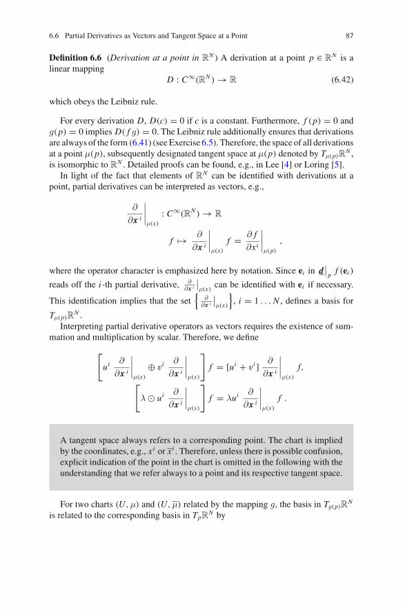
6.6 Partial Derivatives as Vectors and Tangent Space at a Point 87
Definition 6.6 (Derivation at a point in RN ) A derivation at a point p ∈ R
N is alinear mapping
D : C∞(RN ) → R (6.42)
which obeys the Leibniz rule.
For every derivation D, D(c) = 0 if c is a constant. Furthermore, f (p) = 0 andg(p) = 0 implies D( f g) = 0. The Leibniz rule additionally ensures that derivationsare always of the form (6.41) (seeExercise 6.5). Therefore, the space of all derivationsat a point μ(p), subsequently designated tangent space at μ(p) denoted by Tμ(p)R
N ,is isomorphic to RN . Detailed proofs can be found, e.g., in Lee [4] or Loring [5].
In light of the fact that elements of RN can be identified with derivations at apoint, partial derivatives can be interpreted as vectors, e.g.,
∂
∂x i
∣∣∣∣μ(x)
: C∞(RN ) → R
f �→ ∂
∂x i
∣∣∣∣μ(x)
f = ∂ f
∂xi
∣∣∣∣μ(p)
,
where the operator character is emphasized here by notation. Since ei in d˜
∣∣pf (ei )
reads off the i-th partial derivative, ∂∂x i
∣∣μ(x)
can be identified with ei if necessary.
This identification implies that the set{
∂∂x i
∣∣μ(x)
}
, i = 1 . . . N , defines a basis for
Tμ(p)RN .
Interpreting partial derivative operators as vectors requires the existence of sum-mation and multiplication by scalar. Therefore, we define
[
ui∂
∂x i
∣∣∣∣μ(x)
⊕ vi ∂
∂x i
∣∣∣∣μ(x)
]
f = [ui + vi ] ∂
∂x i
∣∣∣∣μ(x)
f,
[
λ ui∂
∂x i
∣∣∣∣μ(x)
]
f = λui∂
∂x i
∣∣∣∣μ(x)
f .
A tangent space always refers to a corresponding point. The chart is impliedby the coordinates, e.g., xi or xi . Therefore, unless there is possible confusion,explicit indication of the point in the chart is omitted in the following with theunderstanding that we refer always to a point and its respective tangent space.
For two charts (U,μ) and (U,μ) related by the mapping g, the basis in Tg(p)RN
is related to the corresponding basis in TpRN by

88 6 Tensor Analysis in Euclidean Space
g�
(∂
∂x i
)
= ∂xk
∂xi∂
∂x k and g−1�
(∂
∂x i
)
= ∂xk
∂xi∂
∂x k. (6.43)
Furthermore, given a vector u ∈ Tg(p)RN as a push forward of a vector u ∈ TpR
N
and considering
g�(u) = uig�
(∂
∂x i
)
= ui∂xk
∂xi∂
∂x k = ui∂
∂x i
yields
ui = ∂xi
∂xkuk
for the transformation of the coordinates.In order to find a corresponding representation for elements of the dual space
T ∗pR
k , we evaluate the gradient of the i-th coordinate function according to (6.15):
d˜
xi = ∂xi
∂xke˜
k = δik e˜
k = e˜
i .
Therefore,d˜
xi : TpRk → R ,
where d˜
xi ∈ T ∗pR
k can be identified with e˜
i if necessary. The identification of thebase vectors and dual base vectors with ei and e
˜
i , respectively, implies
⟨
d˜
xi ,∂
∂x k
⟩
= δik ,
and since, analogously,
⟨
d˜
xi ,∂
∂x k
⟩
= δik
holds, the pull back relations for the corresponding dual vectors
(g−1)�(
d˜
xi) = ∂xi
∂xkd˜
x k , g�(
d˜
xi) = ∂xi
∂xkd˜
xk
can be deduced by taking into account (6.43). Finally, d˜
f can be encoded by
d˜
f = ∂ f
∂xke˜
i = ∂ f
∂xkd˜
xi .

6.6 Partial Derivatives as Vectors and Tangent Space at a Point 89
Box 6.6.1 Summary regarding push forward and pull back for charts (U,μ)
with coordinates xi and (U,μ) with coordinates xi related by g.
g�
(∂
∂x i
) = ∂xk
∂xi∂
∂x k g−1�
(∂
∂x i
)
= ∂xk
∂xi∂
∂x k
g�(
d˜
xi) = ∂xi
∂xk d˜
xk (g−1)�(
d˜
xi) = ∂xi
∂xkd˜
xk
⟨∂
∂x i , d˜
xk⟩ = δki
⟨∂
∂x i , d˜
xk⟩
= δki
Given A = (X,V, ✛ ) and U ⊂ X . The tangent space at a point p in U , TpA isrelated to the tangent space at the image of p in a chart (X,U ) by the push forwardunder μ−1 at μ(p). A basis in Tμ(p)R
N induces a basis ∂ i |p in TpA given by
∂ i |p = μ−1�
(
∂
∂x i
∣∣∣∣μ(p)
)
. (6.44)
From RN ∼= V and Tμ(p)R
N ∼= RN , we deduce TpA ∼= V .
At the end of this section, a property of affine respectively euclidean spaces calledabsolute parallelism is discussed in terms of tangent spaces at points.
Definition 6.7 (Absolute parallelism) Given an affine space A = (X,V, ✛ ). Twovectors u and v where u ∈ TpA and v ∈ TqA are parallel if their coordinates withrespect to a basis {gi } ∈ V are equal.
6.7 Curvilinear Coordinates and Covariant Derivative
Within this section, the following situation is considered. Given a euclidean spaceE = (X,V, ✛ ) and a global affine chart (X,μ). To adapt, for instance, to the geom-etry of a specific problem, a nonlinear chart (U,μ) with U ⊂ X is used in addition.This procedure is known as curvilinear coordinates since the images of the coordi-nate lines of (U,μ) in (X,μ) appear as curved lines. In E , a vector field W exists,and the respective push forwards in the charts are denoted by w and w.
The aim is to determine thederivative ofW along a curveΓ : R → X at p = Γ (t0)bymeans of the respective computation in chart (U,μ). The images ofΓ in the chartsare γ and γ.
E , as well as (X,μ) and (U,μ), disposes of an absolute parallelism. However,while E and (X,μ) are compatible in this respect, the parallelism of (U,μ) is incom-patible with the remaining two due to the nonlinearity of μ. Therefore, we define the

90 6 Tensor Analysis in Euclidean Space
derivative
∇γw = limt→t0
1
t
[
(w ◦ γ(t0 + t))|| − w ◦ γ(t0)]
, (6.45)
where ()|| stands for “transporting in parallel” from Tγ(t0+t)RN to Tγ(t0)R
N , but interms of the parallelism in E . Using the representation of vectors by means of coordi-nates and basis, it is sufficient to discuss the parallel transport of ∂
∂x i from Tγ(t0+t)RN
to Tγ(t0)RN . This should yield a relation
(
∂
∂x i
∣∣∣∣γ(t0+t)
)
||= aki (t0 + t)
∂
∂x k
∣∣∣∣γ(t0)
. (6.46)
In order to determine the aki , the following scheme is used:
1. push forward ∂∂x i at γ(t0 + t) under g−1
2. parallel transport of the result of step 1 from Tγ(t0+t)RN to Tγ(t0)R
N by the identitymap Id
3. express the result of step 2 in terms of the push forwards of the base vectors ∂∂x i
under g−1 at γ(t0)4. push forward the result of step 3 under g at γ(t0)
which is also sketched in Fig. 6.3.Performing step 1 and denoting the result of the respective push forward by
Gi |γ(t0+t), we have
x1
x2
x1
x2
γ(t0)γ(t0 + t)
γ(t0)
γ(t0 + t)
g−1
g
g
g−1
Id a
∂∂x 1 γ(t0)
∂∂x 2 γ(t0)
∂∂x 1 γ(t0+t)
∂∂x 2 γ(t0+t)
∂∂x 1 γ(t0)
∂∂x 2 γ(t0)
∂∂x 1 γ(t0+t)
∂∂x 2 γ(t0+t)
Tγ(t0)R2
Tγ(t0)R2
Tγ(t0+t)R2 Tγ(t0+t)R
2
Fig. 6.3 Sketch of parallel transport in (U, μ) according to the notion of parallelism in E

6.7 Curvilinear Coordinates and Covariant Derivative 91
x1 = r
x2 = ϕ
x1
x2
γ(τ) γ(τ)
g−1
e1
e2
e1
e1G1|γ(τ)
G2|γ(τ)
Fig. 6.4 Meaning of the vectors Gi for Example 6.1. Regarding chart (X,μ) (LHS), the ei can beidentified with ∂
∂x i whereas they are identified with respect to chart (U, μ) (RHS) with ∂∂x i
Gi |γ(t0+t) = g−1�
(∂
∂x i
)
γ(t0+t)
= ∂xm
∂xi
∣∣∣∣γ(t0+t)
∂
∂x m.
Regarding the meaning of Gi , see also Fig. 6.4. Step 2 is trivial, and for step 3,
Gi |γ(t0) = g−1�
(∂
∂x i
)
γ(t0)
= ∂xm
∂xi
∣∣∣∣γ(t0)
∂
∂x m
is required. From the above equation,
∂
∂x m= ∂x j
∂xm
∣∣∣∣∣γ(t0)
G j
∣∣γ(t0)
can be deduced, by which (6.7) can be written as
Gi |γ(t0+t) = ∂xm
∂xi
∣∣∣∣γ(t0+t)
∂x j
∂xm
∣∣∣∣∣γ(t0)
G j
∣∣γ(t0)
= a ji (γ(t0 + t)) G j
∣∣γ(t0)
.
Performing step 4 with the result above as input yields (6.46).Based on the results obtained above, (6.45) reads as
∇γw = limt→t0
1
t
[
wi ◦ γ(t0 + t)ami (γ(t0 + t)) − wm ◦ γ(t0)] ∂
∂x m .
Taylor expansion of the termswithin brackets and performing the limit process resultseventually in

92 6 Tensor Analysis in Euclidean Space
∇γw =[∂w i
∂x j γj + w kΓ i
kq γq]
∂
∂x i , (6.47)
which is called the covariant derivative of a vector field along a curve γ evaluated atγ(t0).
The so-called Christoffel-symbols at γ(t0) are given by
Γ mik
∣∣γ(t0)
= ∂αmi
∂xk
∣∣∣∣γ(t0)
= ∂2x j
∂xi∂xk
∣∣∣∣γ(t0)
∂xm
∂x j
∣∣∣∣γ(t0)
.
According to the point of view introduced within this section, the αmi in (6.46)
relate, i.e. connect, tangent spaces of different points with each other. The Christoffelsymbols are a linearization of this connection valid in the vicinity of a consideredpoint. Therefore, they are also known as coefficients of a so-called affine connection.It should be noted that the Γ m
ik are not the coordinates of a third order tensor. Foraffine chart relations, the Γ m
ik vanish. Hence, the covariant derivative generalizes thedirectional derivative for nonlinear chart relations and contains affine chart relationsas a special case.
The γkin (6.47) are the coordinates of the tangent vectors of γ at γ(t0). This
indicates that (6.47) can be generalized as covariant derivative of a vector field wwith respect to another vector field v,
∇vw =[∂w i
∂x j v j + w kΓ ikqv
q
]∂
∂x i . (6.48)
The following properties of the covariant derivative can be deduced from itsdefinition (6.48):
∇Φu+Ψ vW = Φ ∇uW + Ψ ∇vW
∇u(αW + βV) = α∇u(W) + β∇u(V)
∇u(ΦW) = ∇u(Φ)W + Φ∇u(W) ,
where Φ and Ψ are scalar fields and α and β are real numbers.
Remark 6.1 Inspired by Gründeman [2], the derivation of the covariant derivativewithin this section differs from expositions often found in the context of curvilinearcoordinates (see, e.g., Itskov [3], Fleisch [1] or Neuenschwander [6]). This is moti-vated by the objective of showing how this subject is related to Chap.7. First of all,computation of the connection coefficients within this section was only possible dueto the information that the space in question is euclidean. Furthermore, the informa-tion about parallel transport defines the connection coefficients Γ i
kq , and vice versa.On the other hand, a covariant derivative defines the parallel transport, etc., whichalready indicates at this point the equivalence of these concepts. Furthermore, it is

6.7 Curvilinear Coordinates and Covariant Derivative 93
important to note that normed versions of theGi are used most often in the literature,which has to be taken into account when comparing results.
6.8 Differential Forms inRRRN and Integration
According to Sect. 4.5, the gradient of a function f , d˜
f , defined on RN , is a 1-form.In order to take account of the specific nature of d
˜
f , it is called a differential 1-form.Given two differential 1-forms, d
˜
f and d˜
g, a differential 2-form
ω˜
= d˜
f ∧ d˜
g
can be constructed by means of the exterior product. However, more general objectsare possible, and the set of all possible ω
˜= ωi d
˜
xi forms a space Ω1, whereas theω˜
= ωi j d˜
xi ∧ d˜
x j form a space Ω2, etc. The distinction between Λk introduced inSect. 4.5 and Ωk is that Ωk is related to the tangent space at a point TpR
N .It turns out that differential forms are the proper objects for integration, since
integration defined by means of forms is applicable in more general contexts. There-fore, in what follows, a reformulation of integration based on differential forms isdiscussed. We start with an extremely simple case in R
2.Given a two form
ω˜
= f (x1, x2) d˜
x1 ∧ d˜
x2 (6.49)
at every point p which belongs to a rectangular domain [0, 1] × [0, 1] in R2. The
function f (x1, x2) is supposed to be continuous. Performing at some point p =(p1, p2)
ω˜
(
Δx1∂
∂x 1,Δx2
∂
∂x 2
)
= f (p1, p2)Δx1Δx2
with Δx1,Δx2 ∈ R not only indicates how integration based on differential formsshould be designed, it also reveals the relation with traditional integration in R
N .Technically, we define a grid of points p[m,n] with coordinates
p[m,n] = ((m − 1)Δx1, (n − 1)Δx2) .
For simplicity, we use
Δx1 = Δx2 = 1
N,

94 6 Tensor Analysis in Euclidean Space
and define
∫
[0,1]×[0,1]ω˜
= limN→∞
N+1∑
m=1
N+1∑
n=1
ω˜
[m,n](
Δx1∂
∂x 1,Δx2
∂
∂x 2
)
= limN→∞
N+1∑
m=1
N+1∑
n=1
f (p[m,n])Δx1Δx2 ,
which ensures that regarding RN integration by means of forms coincides with stan-dard integration, e.g.,
∫
D
ω˜
=∫
D
f (x1, x2)dx1dx2 (6.50)
for a 2-form (6.49) in R2.A rather simple approach to handling more complicated domains of integration
D is to replace the argument ω˜by Dω
˜with
D ={
1 p ∈ D0 p /∈ D
,
the integration∫ Dω
˜then being performed with respect to a domain which
includes D.In order to ensure that the result of integration does not depend on the choice of
a particular chart, the pull back operation already discussed for 1-forms (see (6.24))has to be generalized for differential n-forms. We consider the setting sketched inFig. 6.3 and a 2-form in chart (U,μ),
ω˜
= ω(x1, x2) d˜
x1 ∧ d˜
x2 .
The pull back of ω˜under g is defined by
g�ω˜
(u, v) = ω˜
(g�(u), g�(v)) , (6.51)
i.e., the pull back g�ω˜
should give the same result when evaluated for the vectors uand v as ω
˜when evaluated for the respective push forwards. The push forwards of
u and v read as (see Box 6.6.1)
g�(u) = [
u1β11 + u2β1
2
] ∂
∂x 1 + [
u1β12 + u2β2
2
] ∂
∂x 2
g�(v) = [
v1β11 + v2β1
2
] ∂
∂x 1 + [
v1β12 + v2β2
2
] ∂
∂x 2
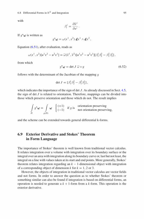
6.8 Differential Forms in RN and Integration 95
with
βji = ∂x j
∂xi.
If g�ω˜is written as
g�ω˜
= ω(x1, x2) d˜
x1 ∧ d˜
x2 ,
Equation (6.51), after evaluation, reads as
ω(x1, x2)[u1v2 − u2v1] = ω(x1, x2)[u1v2 − u2v1][β11β
22 − β2
1β12 ] ,
from whichg�ω
˜= det J ω ◦ g (6.52)
follows with the determinant of the Jacobian of the mapping g
det J = [β11β
22 − β2
1β12 ] ,
which indicates the importance of the sign of det J . As already discussed in Sect. 4.5,the sign of det J is related to orientation. Therefore, mappings can be divided intothose which preserve orientation and those which do not. The result implies
∫
D
g�ω˜
=∫
g(D)
ω˜
{
(+1)(−1)
if g isorientation preservingnot orientation preserving,
and the scheme can be extended towards general differential k-forms.
6.9 Exterior Derivative and Stokes’ Theoremin Form Language
The importance of Stokes’ theorem is well known from traditional vector calculus.It relates integration over a volume with integration over its boundary surface or theintegral over an areawith integration along its boundary curve or, last but not least, theintegral on a line with values taken at its start and end points. More generally, Stokes’theorem relates integration regarding an k − 1-dimensional object with integrationof a corresponding object of dimension k for k = 1, 2 or 3.
However, the objects of integration in traditional vector calculus are vector fieldsand not forms. In order to answer the question as to whether Stokes’ theorem orsomething similar can also be found if integration is based on differential forms, anoperation is needed to generate a k + 1-form from a k-form. This operation is theexterior derivative.

96 6 Tensor Analysis in Euclidean Space
The operation d˜
f generates a 1-form from a function. Interpreting a function as a0-form, there is a certain temptation to proceed this way. However, evaluating d
˜
(d˜
f )yields
d˜
(d˜
f ) = ∂2 f
∂xi∂x jd˜
xi ⊗ d˜
x j ,
which is not an alternating 2-form, and therefore not suitable as an object of inte-gration. However, the result of an operation which takes a differential form as itsargument and is defined as
d := d˜
∧ (6.53)
is again an alternating differential form. For instance,
d(d˜
f ) = d
(∂ f
∂xid˜
xi)
= ∂2 f
∂xi∂xkd˜
xk ∧ d˜
xi .
By means of the exterior derivative (6.53), Stokes’ theorem can be stated in formlanguage as follows:
∫
∂D
ω˜
=∫
D
dω˜
(6.54)
for a differential form defined on the domain D where ∂D is the boundary of D.In order to see how (6.54) works, we consider the square [0, 1] × [0, 1] in R2 and adifferential 1-form
ω˜
= ω1(x1, x2)d
˜
x1 + ω2(x1, x2)d
˜
x2 .
The exterior derivative of ω˜reads as
dω˜
= ∂
∂xkd˜
xk ∧ ω˜
= ∂ω1
∂x2d˜
x2 ∧ d˜
x1 + ∂ω2
∂x1d˜
x1 ∧ d˜
x2
or, respectively,
dω˜
=[∂ω2
∂x1− ∂ω1
∂x2
]
d˜
x1 ∧ d˜
x2 .
Integrating according to (6.50), taking into account
1∫
x2=0
1∫
x1=0
∂
∂x1ω2(x
1, x2)dx1dx2 =1∫
x2=0
[
ω2(1, x2) − ω2(0, x
2)]
dx2
eventually yields the integral of ω˜along the boundary of the square according to the
orientation in Fig. 6.5 (left).Stokes’ theorem in form language reveals one of the advantages of integration
based on differential forms. There is one general formula no matter the dimension

6.9 Exterior Derivative and Stokes’ Theorem in Form Language 97
Fig. 6.5 Two possibleorientations for the unitsquare
of the problem. General proofs of Stokes’ theorem can be found, e.g., in Lee [4] andmany other texts on differentiable manifolds.
The exterior derivative is linear in both arguments and has, in addition, the fol-lowing properties:
d(ω˜
∧ η˜
) = dω˜
∧ η˜
+ (−1)rqω˜
∧ dη˜
,
d(dω˜
) = 0 ,
for ω˜
∈ Ωr and η˜
∈ Ωq at some point p. Furthermore, the exterior derivative com-mutes with the pull back, i.e.,
d(g∗ω˜
) = g∗(dω˜
) .
For a 0-form f and a 1-form η˜
, it can be shown that d f = d˜
f , ∗dη˜
, and ∗d ∗ η˜correspond to the operations grad, curl and div of classical vector calculus.
Remark 6.2 The operations curl and divmentioned at the end of Sect. 6.3 are definedfor vector fields. Vector fields, on the other hand, are the objects of integration intraditional vector calculus. However, if integration is performed entirely by meansof differential forms, curl and div of vector fields are of no use any more.
Exercises
6.1 Compute d |x0 f for f = x2 according to (6.6).
6.2 Compute d |x0=0 f for f = |x | according to (6.6) for h = −1 and h = 1. Is d |0|x |linear wrt. h?
6.3 Show that (6.6) is equivalent to
d |x0 f =[d
dε[ f (x0 + εh) − f (x0)]
]
ε=0
.
Hint: use Taylor series expansion.
6.4 Derive a generalization of the chain rule (6.9) for RN .

98 6 Tensor Analysis in Euclidean Space
6.5 Given two functions Φ and Ψ defined in R2. Show that the mapping
f �→ limt→0
1
t[ f (p ✛ th) − f (p)]
with f = ΦΨ obeys the Leibniz rule by applying Taylor series expansion.
6.6 Show that a derivation D at a point p ∈ RN is always of the form
D( f ) = ∂ f
∂xk
∣∣∣∣p
vk
for any f ∈ C∞(RN ).Hint: Use Taylor series with remainder
f (x) = f (p) + ∂ f
∂xi
∣∣∣∣p
[xi − pi ] + R(x)[xi − pi ]
for representing f at points x close to p and apply D. Take into account that R(p)= 0.
6.7 For the Example 6.1, determine the push forward of the vector field
w = x1∂
∂x 1+ x2
∂
∂x 2
from (U,μ) to (U,μ) at x1 = x2 = 1.
6.8 Given ω˜
= ω1(x1, x2)d˜
x1 + ω2(x1, x2)d˜
x2 in R2. Evaluate∫
∂D
ω˜
= ∫
Ddω˜with
D the unit square using the orientation sketched in Fig. 6.5 (right).
References
1. Fleisch D (2011) A student’s guide to vectors and tensors. Cambridge University Press,Cambridge
2. Gründeman H (2015) HS Mittweida, private communication3. ItskovM (2012) Tensor algebra and tensor analysis for engineers: with applications to continuum
mechanics. Mathematical engineering. Springer, Berlin4. LeeM (2002) Introduction to smoothmanifolds. Graduate texts inmathematics. Springer, Berlin5. Loring WT (2011) An introduction to manifolds, 2nd edn. Universitext. Springer, New York6. Neuenschwander D (2014) Tensor calculus for physics: a concise guide. Johns Hopkins
University Press, Baltimore
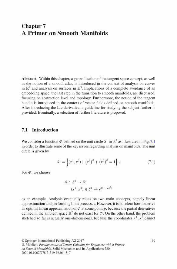
Chapter 7A Primer on Smooth Manifolds
Abstract Within this chapter, a generalization of the tangent space concept, as wellas the notion of a smooth atlas, is introduced in the context of analysis on curvesin R
2 and analysis on surfaces in R3. Implications of a complete avoidance of an
embedding space, the last step in the transition to smooth manifolds, are discussed,focusing on abstraction level and topology. Furthermore, the notion of the tangentbundle is introduced in the context of vector fields defined on smooth manifolds.After introducing the Lie derivative, a guideline for studying the subject further isprovided. Eventually, a selection of further literature is proposed.
7.1 Introduction
We consider a function Φ defined on the unit circle S1 in R2 as illustrated in Fig. 7.1in order to illustrate some of the key issues regarding analysis on manifolds. The unitcircle is given by
S1 ={(x1, x2) | (
x1)2 + (
x2)2 = 1
}. (7.1)
For Φ, we choose
Φ : S1 → R
(x1, x2) ∈ S1 �→ e(x1+2x2)
as an example. Analysis eventually relies on two main concepts, namely linearapproximation and performing limit processes. However, it is not clear how to derivean optimal linear approximation ofΦ at some point p, because the partial derivativesdefined in the ambient space R2 do not exist for Φ. On the other hand, the problemsketched so far is actually one-dimensional, because the coordinates x1, x2 cannot
© Springer International Publishing AG 2017U. Mühlich, Fundamentals of Tensor Calculus for Engineers with a Primeron Smooth Manifolds, Solid Mechanics and Its Applications 230,DOI 10.1007/978-3-319-56264-3_7
99
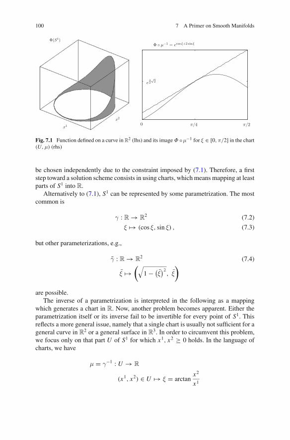
100 7 A Primer on Smooth Manifolds
x1
x2
Φ(S1)
0 π/4 π/2
Φ ◦ μ−1 = ecos ξ+2 sin ξ
e32
√2
Fig. 7.1 Function defined on a curve in R2 (lhs) and its image Φ ◦μ−1 for ξ ∈ [0,π/2] in the chart(U,μ) (rhs)
be chosen independently due to the constraint imposed by (7.1). Therefore, a firststep toward a solution scheme consists in using charts, which means mapping at leastparts of S1 into R.
Alternatively to (7.1), S1 can be represented by some parametrization. The mostcommon is
γ : R → R2 (7.2)
ξ �→ (cos ξ, sin ξ) , (7.3)
but other parameterizations, e.g.,
γ : R → R2 (7.4)
ξ �→(√
1 − (ξ)2
, ξ
)
are possible.The inverse of a parametrization is interpreted in the following as a mapping
which generates a chart in R. Now, another problem becomes apparent. Either theparametrization itself or its inverse fail to be invertible for every point of S1. Thisreflects a more general issue, namely that a single chart is usually not sufficient for ageneral curve in R2 or a general surface in R3. In order to circumvent this problem,we focus only on that part U of S1 for which x1, x2 ≥ 0 holds. In the language ofcharts, we have
μ = γ−1 : U → R
(x1, x2) ∈ U �→ ξ = arctanx2
x1

7.1 Introduction 101
and
μ = γ−1 : U → R
(x1, x2) ∈ U �→ ξ = 1√2
√1 − (
x1)2 + x2 ,
together with μ−1 = γ and μ−1 = γ given by (7.2) and (7.4). The image of Φ in thechart (U,μ) reads as
f = Φ ◦ μ−1 = e(cos ξ+2 sin ξ) ,
whereas the image of Φ in the chart (U, μ) is given by
f = Φ ◦ μ−1 = e√1−(ξ)
2+ξ.
Since f and f are functions of one variable, the derivatives of these functions at thepoint in the charts which correspond to p = ( 12
√2, 1
2
√2) can be determined, and
we obtaind
dξf
∣∣∣∣ξ=π/4
= 1
2
√2e
32
√2 , (7.5)
andd
dξf
∣∣∣∣ξ= 1
2
√2
= e32
√2 . (7.6)
Since Φ(p) = f (μ(p)) = f (μ(p)), one might be tempted to estimate the valueof Φ at a point q, e.g. q = (0, 1) based on a linear approximation of the image of Φ
at p in some chart. For the chart (U,μ) the linear approximation of f reads as
dμ(p) f (h) = 1
2
√2e
32
√2 h ,
and setting h = μ(q) − μ(p) = π4 yields the estimate
f (μ(q)) ≈ f (μ(p)) + π
8
√2e
32
√2 .
For the chart (U, μ), the estimate
f (μ(q)) ≈ f (μ(p)) + e32
√2
is obtained, fromwhich it can be seen that results generated this way are chart depen-dent, and therefore completely useless. This chart dependence is just a manifestationof a deeper problem.
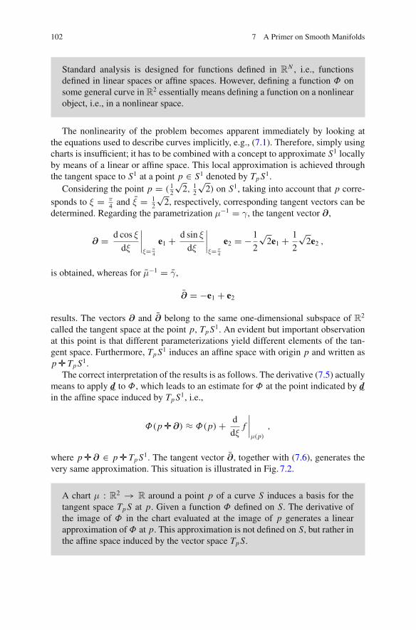
102 7 A Primer on Smooth Manifolds
Standard analysis is designed for functions defined in RN , i.e., functions
defined in linear spaces or affine spaces. However, defining a function Φ onsome general curve in R2 essentially means defining a function on a nonlinearobject, i.e., in a nonlinear space.
The nonlinearity of the problem becomes apparent immediately by looking atthe equations used to describe curves implicitly, e.g., (7.1). Therefore, simply usingcharts is insufficient; it has to be combined with a concept to approximate S1 locallyby means of a linear or affine space. This local approximation is achieved throughthe tangent space to S1 at a point p ∈ S1 denoted by TpS1.
Considering the point p = ( 12
√2, 1
2
√2) on S1, taking into account that p corre-
sponds to ξ = π4 and ξ = 1
2
√2, respectively, corresponding tangent vectors can be
determined. Regarding the parametrization μ−1 = γ, the tangent vector ∂,
∂ = d cos ξ
dξ
∣∣∣∣ξ= π
4
e1 + d sin ξ
dξ
∣∣∣∣ξ= π
4
e2 = −1
2
√2e1 + 1
2
√2e2 ,
is obtained, whereas for μ−1 = γ,
∂ = −e1 + e2
results. The vectors ∂ and ∂ belong to the same one-dimensional subspace of R2
called the tangent space at the point p, TpS1. An evident but important observationat this point is that different parameterizations yield different elements of the tan-gent space. Furthermore, TpS1 induces an affine space with origin p and written asp ✛ TpS1.
The correct interpretation of the results is as follows. The derivative (7.5) actuallymeans to apply d˜ to Φ, which leads to an estimate for Φ at the point indicated by d˜in the affine space induced by TpS1, i.e.,
Φ(p ✛ ∂) ≈ Φ(p) + d
dξf
∣∣∣∣μ(p)
,
where p ✛ ∂ ∈ p ✛ TpS1. The tangent vector ∂, together with (7.6), generates thevery same approximation. This situation is illustrated in Fig. 7.2.
A chart μ : R2 → R around a point p of a curve S induces a basis for thetangent space TpS at p. Given a function Φ defined on S. The derivative ofthe image of Φ in the chart evaluated at the image of p generates a linearapproximation of Φ at p. This approximation is not defined on S, but rather inthe affine space induced by the vector space TpS.

7.1 Introduction 103
p
x1
x2
Γ
∂∂
p 1 √2
∂
∂0
Φ(p)
Φ(p) + ∂Φ
Φ(p) + ∂Φ
Fig. 7.2 Curve S1 inR2, togetherwith the tangent space at point p, TpS1 (LHS). Different base vec-tors of TpS1 induced by different charts are sketched as well. Furthermore, the linear approximationof a function Φ in the affine space induced by TpS1 is plotted (RHS). See also Fig. 7.1
The example already illustrates two of the key ideas of smooth manifolds, namelycharts and tangent space. However, due to its simplicity, not everything can be illus-trated properly by it. Therefore, we proceed with analysis on surfaces in R3.
7.2 Basic Concepts Regarding Analysis on Surfaces inRRR3
Within this section, functions defined on surfaces in R3 are considered. S is used
to indicate a general surface and Φ denotes a function defined on it. The aim is todiscuss decisive concepts like charts, atlases, and tangent space to a point of S in thiscontext. Since we can still rely on the ambient spaceR3, continuity, and convergencecan still be discussed, for instance, using the metric of the ambient space togetherwith the implicit representation of S. Therefore, topological aspects do not have tobe discussed yet.
The unit sphere S2 in R3
S2 ={(y1, y2, y3) | (
y1)2 + (
y2)2 + (
y3)2 − 1 = 0
}(7.7)
serves as specific example to illustrate certain concepts. S2 can be represented by two-dimensional charts. A possible collection of charts (U,μ) and (U, μ) is generatedby the mappings
μ : S2 → R2
(y1, y2, y3 = −1) ∈ S2 �→(x1 = y1
1 + y3, x2 = y2
1 + y3
)
μ : S2 → R2
(y1, y2, y3 = +1) ∈ S2 �→(x1 = y1
1 − y3, x2 = y2
1 − y3
),
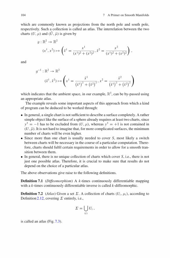
104 7 A Primer on Smooth Manifolds
which are commonly known as projections from the north pole and south pole,respectively. Such a collection is called an atlas. The interrelation between the twocharts (U,μ) and (U , μ) is given by
g : R2 → R2
(x1, x2) �→(x1 = x1
(x1)2 + (x2)2, x2 = x2
(x1)2 + (x2)2
),
and
g−1 : R2 → R2
(x1, x2) �→(x1 = x1(
x1)2 + (
x2)2 , x2 = x2(
x1)2 + (
x2)2
)
which indicates that the ambient space, in our example, R3, can be by-passed usingan appropriate atlas.
The example reveals some important aspects of this approach from which a kindof program can be deduced to be worked through:
• In general, a single chart is not sufficient to describe a surface completely. A rathersimple object like the surface of a sphere already requires at least two charts, sincey3 = −1 has to be excluded from (U,μ), whereas y3 = +1 is not contained in(U, μ). It is not hard to imagine that, for more complicated surfaces, the minimumnumber of charts will be even higher.
• Since more than one chart is usually needed to cover S, most likely a switchbetween charts will be necessary in the course of a particular computation. There-fore, charts should fulfil certain requirements in order to allow for a smooth tran-sition between them.
• In general, there is no unique collection of charts which cover S, i.e., there is notjust one possible atlas. Therefore, it is crucial to make sure that results do notdepend on the choice of a particular atlas.
The above observations give raise to the following definitions.
Definition 7.1 (Diffeomorphism) A k-times continuously differentiable mappingwith a k-times continuously differentiable inverse is called k-diffeomorphic.
Definition 7.2 (Atlas) Given a set Σ . A collection of charts (Ui ,μi ), according toDefinition2.12, covering Σ entirely, i.e.,
Σ =⋃(i)
Ui ,
is called an atlas (Fig. 7.3).

7.2 Basic Concepts Regarding Analysis on Surfaces in R3 105
x1
x2
x 1
x 2
p r
sq
μ(p)
μ(q)
μ(r)
μ(s)
μ(p)μ(q)
μ(r) μ(s)
g
g−1
μ μ
f = Φ ◦ μ−1f = Φ ◦ μ−1
Fig. 7.3 Surface with a function defined on it and two possible charts of the neighborhood of apoint p on the surface
Definition 7.3 (Ck-Atlas) If for any two charts (Ui ,μi ) and (Uk,μk) of an atlas A,the mappings
μk ◦ μ−1i
are k-diffeomorphic, then A is a Ck-atlas. A smooth atlas is a C∞-atlas.
Definition 7.4 (Set of continuously differentiable functions on a set Σ) The setof all functions f : Σ → R whose images in the charts have continuous partialderivatives up to order k is called Ck(Σ).
Please note that the above definitions are not limited to sets which form surfacesinRn . In consideration of the topics discussed within the subsequent sections, a moregeneral point of view is already employed here.
As already discussed within the previous section, the concept of a linearizationof S at a point p on S is required in order to proceed. Tangent vectors at points ofa surface can be defined as vectors tangent to curves passing through p. Given acurve Γ ,
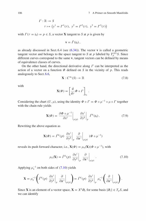
106 7 A Primer on Smooth Manifolds
Γ : R → S
τ �→ (y1 = Γ 1(τ ), y2 = Γ 2(τ ), y3 = Γ 3(τ )
)
with Γ (τ = t0) = p ∈ S, a vector X tangent to S at p is given by
v = Γ (t0) ,
as already discussed in Sect. 6.4 (see (6.34)). The vector v is called a geometrictangent vector and belongs to the space tangent to S at p labeled by T (G)
p S. Sincedifferent curves correspond to the same v, tangent vectors can be defined by meansof equivalence classes of curves.
On the other hand, the directional derivative along Γ can be interpreted as theaction of a vector on a function Φ defined on S in the vicinity of p. This readsanalogously to Sect. 6.6,
X : C∞(S) → R (7.8)
with
X(Φ) =[d
dτΦ ◦ Γ
]
t0
.
Considering the chart (U,μ), using the identity Φ ◦ Γ = Φ ◦ μ−1 ◦ μ ◦ Γ togetherwith the chain rule yields
X(Φ) = ∂Φ ◦ μ−1
∂xi
∣∣∣∣μ(p)
∂xi
∂yk
∣∣∣∣p
Γ k(t0) . (7.9)
Rewriting the above equation as
X(Φ) = Γ k(p)∂xi
∂yk
∣∣∣∣p
∂
∂x i
∣∣∣∣μ(p)
(Φ ◦ μ−1)
reveals its push forward character, i.e., X(Φ) = μ�(X)(Φ ◦ μ−1), with
μ�(X) = Γ k(p)∂xi
∂yk
∣∣∣∣p
∂
∂x i
∣∣∣∣μ(p)
. (7.10)
Applying μ−1� on both sides of (7.10) yields
X = μ−1�
(Γ k(p)
∂xi
∂yk
∣∣∣∣p
∂
∂x i
∣∣∣∣μ(p)
)= Γ k(p)
∂xi
∂yk
∣∣∣∣p
μ−1�
(∂
∂x i
∣∣∣∣μ(p)
).
Since X is an element of a vector space, X = Xk∂k for some basis {∂ i } ∈ TpS, andwe can identify

7.2 Basic Concepts Regarding Analysis on Surfaces in RRR3 107
∂ i = μ−1�
(∂
∂x i
∣∣∣∣μ(p)
), Xi = Γ k(p)
∂xi
∂yk
∣∣∣∣p
.
Using another chart (U, μ), the same line of arguments yields the identification
∂ i = μ−1�
(∂
∂ x i
∣∣∣∣μ(p)
), X i = Γ k(p)
∂ x i
∂yk
∣∣∣∣p
,
i.e., different charts induce different bases in TpS. Regarding a basis {∂ i } in TpSinduced by the chart (U,μ) with coordinates xi , the notation
∂
∂x i
∣∣∣∣p
= ∂ i
is also often found in literature. It has the advantage of making the origin of the basisexplicit.
In the previous considerations, we tacitly assumed that addition and multiplica-tion in TpS are defined, because a representation by means of coordinates and basevectors would not otherwise be possible. However, analogously to Sect. 6.6, properdefinitions have to be provided. Hence, we define
[X ⊕ Y] (Φ) = X(Φ) + Y(Φ) (7.11)
[λ � X] (Φ) = λX(Φ) = X(λΦ) (7.12)
for X,Y ∈ TpS, Φ ∈ C∞(S) and λ ∈ R. The definition is only appropriate if it canbe shown that the results of X + Y and λ � X are again elements of TpS.
Furthermore, it can be shown that tangent vectors defined according to (7.8) obeythe Leibniz rule
X(ΦΨ ) = Φ(p)X(Ψ ) + Ψ (p)X(Φ)
for X,Y ∈ TpS.The methodology applied here for the purpose of proceeding toward general
smooth manifolds is somehow similar to the one used in Chap.2 regarding the stepfrommetric spaces to topological spaces. For surfaces in an ambient spaceRn , it canbe shown that TpS is isomorphic to the geometric tangent space at a point p. Just likegeometric tangent vectors, the elements of TpS obey the Leibniz rule. The transitionto smooth manifolds now consist, roughly speaking, in defining a manifold by theexistence of a smooth atlas and tangent vectors at a point p as derivations, henceobjects according to (7.8), (7.11), and (7.12) which obey the Leibniz rule, and noreference to some ambient space is required. This is discussed in more details in theremaining part of this chapter.

108 7 A Primer on Smooth Manifolds
7.3 Transition to Smooth Manifolds
Within the previous sections, we have seen that the ambient space can be bypassed bymeans of an appropriate atlas, i.e., a suitable collection of charts. The total avoidanceof an embedding, i.e., the complete absence of an ambient space, however, alsoimplies the absence of a topology on the set of points S meant to serve as a modelfor physical space. At this point, it is worth noting that without being at least awareof the concept of topological space, it would be difficult to proceed further.
From now on, S refers to a general set, and not just to a set which forms a surfacein R
3. S can be endowed with a topology by means of an atlas A, since the latterconsist of charts which are by definition homeomorphisms.
Definition 7.5 (Topological manifold) A topological manifold M = (S,A) is a setS together with an atlas, according to Definition7.2.
Unfortunately, it is not possible now to define a differentiable or smooth manifoldjust by means of a differentiable atlas, according to Definition7.3. The reason is thatit can not be shown that the topology induced on S by the collection of charts makesS a Hausdorff-space (see, e.g., Crampin and Pirani [1]). Therefore, the Hausdorff-property must form part of the definition.
Definition 7.6 (Smooth manifold) A smooth manifold M = (S,A) is a Hausdorff-space according to Definition2.20, equipped with a C∞ atlas defined by Defini-tion7.3.
In view of the last section, it is more or less obvious that the next step towardcalculus on manifolds will be the definition of a tangent space at a point on amanifold M .
Definition 7.7 (Tangent space at a point p of a smooth manifold) A derivation ata point p on M is a linear mapping X : C∞(M) → R which obeys the Leibniz rule.The set of all derivations at p, together with
[X ⊕ Y] (Φ) = X(Φ) + Y(Φ)
[λ � X] (Φ) = λX(Φ) = X(λΦ)
and Φ ∈ C∞(M), forms a vector space called TpM .
Two goals are achieved by Definition7.7. Firstly, a linearization of M at a pointp is defined without reference to an ambient space. Secondly, if there is an ambientspace, then the well-known case of geometric tangent vectors with all its potentialfor graphical illustration is recovered due to T (G)
p M ∼= TpM . Alternative ways forconstructing a tangent space at a point ofM exist that are all equivalent. The interestedreader is referred, e.g., to Jänich [3].
Consistently, the space of all linear mappings X˜ : TpM → R is called the dualtangent space T ∗
p M or the cotangent space at p.

7.3 Transition to Smooth Manifolds 109
Given two manifolds M and N together with a mapping F : M → N , the pushforward F� of a vector X ∈ TpM is defined analogously to Sect. 6.4 by the condition
X(Φ) = F�(X)(Φ ◦ F−1)
with F�(X) ∈ TF(p)N and Φ ∈ C∞(M). The corresponding condition that definesthe pull back operation, ⟨
F�(Ω˜),X⟩ = ⟨
Ω˜, F�(X)⟩,
also shows the analogy to Sect. 6.4.Due to the avoidance of an embedding, tangent vectors and cotangent vectors
become rather abstract objects. IfM is a smoothmanifold according toDefinition7.6,it is certain that these objects exist. There are operations defined for these objects,e.g., summation, multiplication by a real number, push forward and pull back, butthat is all. Computations have to be performed in charts which looks the same as inthe previous section.
Charts are also used in the context of proofs through the performing of all neces-sary steps in a chart and showing afterwards that the result does not depend on thechoice for a particular chart.
The concept of differentiable/smooth manifolds provides a unifying languagefor analysis in topological spaces with differentiable/smooth structure. Analy-sis in euclidean space is included as a special case for which one global chartis sufficient for performing analysis.
7.4 Tangent Bundle and Vector Fields
Regarding some euclidean space E = (X,V, ✛ ), vector fields can be simply definedas mappings which assign to every point p ∈ X an element of the associated globalvector space V . A basis {gi } for V induces a global chart (X,μ) and continuity anddifferentiability of a vector field V = V i (p)gi can be discussed in terms of thefunctions V i ◦ μ−1 in the global chart.
For a general smoothmanifoldM , this scheme is not applicable due to the absenceof a global vector space. At this point, the concept of the tangent bundle enters thescene. The idea resides in defining a set consisting of the manifold M and all itstangent spaces TpM , i.e.,
T M = {(p, v) | p ∈ M, v ∈ TpM
}.
In order to illustrate certain aspects of this approach, the unit circle S1 in R2
is again used as an example, i.e., M = S1. The tangent bundle T S1 is one of the

110 7 A Primer on Smooth Manifolds
pp qq
rr
TpM
TqM
TrM
Fig. 7.4 Visualization of the tangent bundle for M = S1. Since the visualization shown in theleft picture causes spurious intersections of lines which indicate tangent spaces at different points,the visualization given in the right picture is commonly preferred. The latter allows in addition forinterpretating tangent spaces as fibers attached to the manifold M (see, e.g., Schutz [10])
few cases for which a graphical illustration is possible. As shown in Fig. 7.4, T S1
can be visualized as an infinite cylinder formed by S1, together with a vertical fiberR ∼= TpS1 attached to every point of S1. A smooth vector field on S1 can now beinterpreted as a smooth function on a cylinder, as sketched in Fig. 7.6. However,converting these ideas into a concept which can be applied safely requires someformal work.
Figure7.4 suggests that T S1 is a product space, i.e., T S1 = S1 × R, becausethere exist two natural projections, π : T S1 → S and π∗ : T S1 → R, which arecontinuous. The inverse of π reads off the fiber at p as
π−1(p) = {p} × R ,
whereas the inverse of π∗ provides a circle shifted vertically,
π−1∗ (z) = S1 × {z}
with p ∈ S1 and z ∈ R. Since S1 andR are topological spaces, T S1 can be endowedwith a topology according toSect. 2.5.Moreover, since S1 andR canboth be treated assmoothmanifolds, T S1 is even a productmanifold, T S1 = S1×R. But unfortunately,this does not hold in general, since, for instance, T S2 is not a product manifold.
In order to discuss the implications of the preceding discussion in more detail,while still being able to supplement the discussion with graphical visualizations, weconsider the more general concept of fiber bundles. As before, S1 is used as thebase manifold. A cylinder C of finite height and a Möbius band M as sketched inFig. 7.5 are constructed by combining S1 with the fiber F = (−1, 1) in different

7.4 Tangent Bundle and Vector Fields 111
−1
+1
0
F
p
Fig. 7.5 Sketch of the Möbius band generated from S1 and the fiber F
ways. Both constructions are fiber bundles over the same base manifold. In bothcases, a continuous projection π exists and π−1(p) reads off the fiber associated withp, which is isomorphic to F . However, while for C, the projection π∗ is continuous,there is no such continuous projection for M except for z = 0, z ∈ F . For instance,starting at some p ∈ S1, moving along S1 and choosing z = − 1
2 in every fibereventually delivers a curve with a jump of magnitude 1 at p.
This leads to the conclusion that a common framework for C and M cannot relyon a projection π∗ in a global sense. A projection π, i.e., the projection onto the basemanifold, on the other hand, does not introduce any difficulties. Its inverse at somep ∈ S1 delivers, in both cases, the fiber corresponding to p isomorphic to F . Hence,πcan be used globally. Furthermore, although globally not a product manifold, locally,i.e., in the vicinity of a given point p ∈ S1, M indeed possesses the properties of aproduct manifold as sketched in Fig. 7.5.
Summarizing the discussion so far, a fiber bundle consists at least of the followingingredients: a space E , a base manifold M , a fiber F and a projection π : E → Mwith π−1(p) ∼= F .
Already when introducing the smooth manifold concept, we encountered the ideaof giving up certain concepts globally but retaining them locally. Smooth manifoldsare spaces which cannot be treated globally as affine or euclidean. But, as long asthey can be endowed at least locally with an affine/euclidean structure, a smoothmanifold is, roughly speaking, obtained by gluing together small affine/euclideanpieces. A similar approach is used in the context of fiber bundles. As long as theconcept of a product manifold applies locally, a fiber bundle is obtained by gluingtogether individual product manifolds. The last point indicates that the preliminarysummary with respect to fiber bundles within the previous paragraph is not completeyet, because it does not contain any recipe as to how to glue local parts together.
At this point, we return to our original problem, the tangent bundle T M . Thetangent bundle is a rather special case of a fiber bundle in the sense that the gluingprocedure is already implied by the following definition.
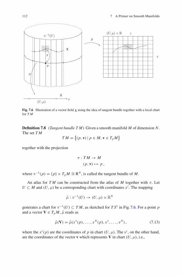
112 7 A Primer on Smooth Manifolds
p
R
(U, μ)
χ
π
μ
μ
x
x
z(U, μ) × Rπ−1(U)
Fig. 7.6 Illustration of a vector field χ using the idea of tangent bundle together with a local chartfor T M
Definition 7.8 (Tangent bundle T M) Given a smooth manifold M of dimension N .The set T M
TM = {(p, v) | p ∈ M, v ∈ TpM
}
together with the projection
π : T M → M
(p, v) �→ p ,
where π−1(p) = {p} × TpM ∼= RN , is called the tangent bundle of M .
An atlas for T M can be constructed from the atlas of M together with π. LetU ⊂ M and (U,μ) be a corresponding chart with coordinates xi . The mapping
μ : π−1(U ) → (U,μ) × RN
generates a chart for π−1(U ) ⊂ T M , as sketched for T S1 in Fig. 7.6. For a point pand a vector V ∈ TpM , μ reads as
μ(V) = μ(x1(p), . . . , xN (p), v1, . . . , vN ) , (7.13)
where the xi (p) are the coordinates of p in chart (U,μ). The vi , on the other hand,are the coordinates of the vector v which represents V in chart (U,μ), i.e.,

7.4 Tangent Bundle and Vector Fields 113
v = vi ∂
∂x i
∣∣∣∣μ(p)
.
Since M is supposed to be a smooth manifold, the atlas for M is a collection ofcharts (Uk,μk) with smooth transition functions (see Definition7.3). Consequently,an atlas for T M can be defined as the collection of charts (π−1(Uk), μk) whichnaturally raises the question regarding the transition between these charts. As (7.13)shows, this transition involves coordinates of points and vectors. With respect to theformer, a smooth transition is ensured by the atlas of M . More interesting is thequestion regarding the vi in (7.13) because it eventually yields the gluing procedure.
Unfortunately, discussing the effect of a chart transition on the vi in (7.13) canmake notation quite cumbersome. We consider two subsets U1 and U2 of M withoverlap U1
⋂U2 and a vector V ∈ TpM with p ∈ U1
⋂U2. In addition, there are
two charts (U1,μ1) and (U2,μ2). The vector which represents V in chart (U1,μ1)
reads as
v1 = vi1
∂
∂xi1
∣∣∣∣μ1(p)
,
whereas for chart (U2,μ2), V is represented by
v2 = vi2
∂
∂xi2
∣∣∣∣μ2(p)
.
A change from chart (U1,μ1) to (U2,μ2) at p requires a push forward of v1 underthe transition map μ2 ◦ μ−1
1 which gives
vi2 = ∂xi2
∂xk1
∣∣∣∣μ2(p)
vk1 = (t12)
ik vk
1
(see as well Box6.6.1). The (t12)ik are the entries of an invertible quadratic matrix t12
of dimension N . Such matrices belong to a specific Lie group, namely the generallinear group GL(N ,R).
This scheme discussed above extends in a straightforward manner to a generalcollection of charts {(Un,μn)}, where transitions with regard to fibers are given bymatrices t
mnwith the following properties:
tmm
= I
tmn
= t−1mn
with the identity matrix I .Similar to the situation in euclidean space, the aim is to define vector fields in the
sense that there is an assignment of a vector to every point p ∈ M . The existenceof vectors is ensured by the tangent space concept. But, since the individual tangent

114 7 A Primer on Smooth Manifolds
spaces are actually unrelated, it does not make sense to assign to a point p a vectorwhich does not belong to the tangent space defined at p.
Definition 7.9 (Vector field on a manifold) A vector field χ on a manifold is amapping
χ : M → T M
p �→ (p, v) ,
which fulfils the condition π ◦ χ = Id.
For a particular point p ∈ M , the condition imposed on vector fields inDefinition7.9 reads as π(χ(p)) = p. This ensures that a vector field indeed assignsto every point p ∈ M not just some vector, but a member of the correspondingtangent space TpM , as demanded earlier.
The definition of vector fields implies that a vector field V is smooth if the coor-dinates of V are smooth functions in the respective smooth charts (see, e.g., inLee [4]).
7.5 Flow of Vector Fields and the Lie Derivative
Due to the avoidance of an ambient space in the definition of smooth manifolds andtheir local linearization, tangent spaces at different points are completely unrelated atthis stage. Without relations between tangent spaces, however, analysis on a smoothmanifold cannot be performed.
Objects available to work with on a smooth manifold M so far are functions andcurves defined on M . On the other hand, curves can be interpreted as integral curvesinduced by a vector field, and vice versa. Exploring this idea further leads to thenotion of the flow of a vector field and the Lie derivative.
The key ideas are explained in the following by means of an elementary examplein R2. Given a vector field
v = v1 e1 + v2 e2 (7.14)
with v1 = a, v2 = b, where a and b are just real numbers. An integral curve Γ ,τ → (x1(τ ), x2(τ )) of this vector field fulfils the condition
dΓ
dτ= Γ = v|Γ (τ ) ,
or, in coordinate representation,
Γ 1 = v1∣∣Γ (τ )
Γ 2 = v2∣∣Γ (τ )
7.5 Flow of Vector Fields and the Lie Derivative 115
for arbitrary values of τ within a given interval. This is a system of ordinary differ-ential equations which can be solved by direct integration, the solution containing Nintegration constants. N coincideswith the dimension of the spacewhich, on the otherhand, equals the number of equations. Focusing on a point p using p = Γ (τ = 0) asthe initial condition to determine the integration constants, yields a particular curvereferring to p. For the example (7.5), this curve reads as
Γp = (aτ + p1, bτ + p2) ,
and a common interpretation of Γp as the trajectory of a material point which atτ = 0 has position p is rather instructive for what follows.
Instead of focusing only on one point, we could also consider a set U of pointsoccupying a connected region in space, or even the whole space. Regarding R
2,the points belonging to U can be identified by their coordinates, x1, x2. In thiscase, χ(τ , x1, x2) is called the flow of the vector field defined on U . In continuummechanics, χ is usually called the motion. For the example (7.14), χ is simply
χ(τ , x1, x2) = (aτ + x1, bτ + x2) .
Evaluating χ for a particular τ = t is then a mapping χt : R2 → R
2. Here, weconsider only a small neighborhoodU(p) of a point p, and thereforeχt : U(p) → U(q),whereU(p),U(q) ∈ R
2. This is illustrated in Fig. 7.7 for a motion a bit more complexthan the one in the example. In the language of continuum mechanics, χt is calleda configuration and χ0 usually serves as a reference configuration for the so-calledLagrangian description.
For a particular point p, χt (p) = Γp(t) = q and χ−t (q) = Γq(−t) = p. On theother hand, p = Γ −1
p (t) and therefore Γ −1p (t) = Γq(−t), and for a set of points
χ−1t (U(q)) = χ−t (U(q)) .
Analogously, for the respective linearized mappings,
(χ−t )�(U(q)) = (χ−1t )�(U(q)) (7.15)
holds.The mapping χt can now be used to relate the tangent spaces at p = Γp(0) and
q = Γp(t) by means of the push forwards induced by χt . This, on the other hand,allows for defining a directional derivative of a vector field w along the integralcurves of another vector field v,
Lvw|p = limt→0
1
t
[(χ−1
t )�(w|Γp(t)) − w|Γp(0)
], (7.16)
known as the Lie derivative. Using the standard basis, we write the push forward(χ−1
s )�(w|Γp(t)) as

116 7 A Primer on Smooth Manifolds
p
q
r
U(p)
U(q)
τ = t
τ = 0
χt
χ−1t
Γp
v|γp(0) v|γp(t)
v|r
Fig. 7.7 Illustration of the flow of a vector field
(χ−1t )�(w|Γp(t)) = αk
i wi (Γ (t)) ek ,
where αki are the coordinates of the push forward and wk(Γ (t)) takes into account
that the coordinates of w change along Γp. Taylor series expansion of wk(Γ (t))yields
wk(Γ (t)) ≈ wk(p) + ∂wk
∂xm
∣∣∣∣p
Γ m(0) t = wk(p) + ∂wk
∂xm
∣∣∣∣p
vm t . (7.17)
For small t , Γp(t) can be approximated by
Γp(t) ≈ p + t v|p ,
but regarding χt , it has to be taken into account that v changes in the vicinity of p.Therefore, χt is approximated for small t by
χt = ξ + t v|ξ ,
where ξ ∈ U(p). The directional derivative
d˜∣∣p χt (h) = lim
s→0
1
s[ξ ✛ sh + tv(ξ ✛ sh) − ξ − tv(ξ)] =
[δki + t
∂vk
∂xi
∣∣∣∣p
]hiek
7.5 Flow of Vector Fields and the Lie Derivative 117
yields the coordinates of the push forward of χt
αki = δki + t
∂vk
∂xi
∣∣∣∣p
,
which can also be obtained just by differentiating the coordinate representation ofχt
χ1t = x1 + tv1(x1, x2)
χ2t = x2 + tv2(x1, x2)
accordingly. Applying (7.15), the coordinates of (χ−t )� read as
αki = δki − t
∂vk
∂xi
∣∣∣∣p
(7.18)
Using (7.17) and (7.18) in (7.16) eventually yields
Lvw|p =[
∂wk
∂xm
∣∣∣∣p
vm(p) − ∂vk
∂xm
∣∣∣∣p
wm(p)
]ek = [v,w]p , (7.19)
where [v,w]p is the so-called Lie bracket evaluated at p.The computation above can be interpreted as a computation performed in a chart
(U,μ). Afterwards, it has to be shown that the result is chart independent. For details,see, e.g., Lee [4].
The Lie bracket is bilinear, and has, in addition, the following properties:
[V,W] = −[W,V][V, [W,Z]] + [W, [Z,V]] + [Z, [V,W]] = 0 ,
which imply the following properties of the Lie derivative:
LVW = −LWV
LV[W,Z] = [LWV,Z] + [W,LVZ]L fVW = (V f )W + f LVW
F�(LVW) = LF�(V)F�(W) ,
where (V f ) is the directional derivative of the function f with respect to V and F�
is the push forward of a mapping F : M → N provided that F is diffeomorphic.It should be noted that the Lie derivative extends to general tensor fields (again see,e.g., Lee [4]).

118 7 A Primer on Smooth Manifolds
For a vector fieldW which depends on time τ , the nonautonomous Lie derivative
LVW = ∂W∂τ
+ LVW
measures the change ofW over timewith respect to the flow induced byV. It iswidelyused, e.g., in continuummechanics in order to measure the change of a quantity overtime in case the support of this quantity changes in time as well, e.g, stress in amoving and deforming body.
7.6 Outlook and Further Reading
The objective of this section is to provide some guidance to the reader regardingthe further exploration of the smooth manifold concept. We intend to give a shortoverview in terms of topics the reader will most likely be confronted with in thisendeavor and to recommend appropriate literature. Regarding the latter, a large num-ber of excellent textbooks exist, many of them in the context of general relativity ortheoretical physics in a broader sense. The selection made here is surely biased bythe accessibility of specific textbooks in libraries and bookshops. It is also a matter oftaste, and therefore, rather subjective. In addition, literature is selected with a mindtoward an audience interested in engineering mechanics, respectively, continuummechanics.
As discussed earlier, tangent spaces on a manifold M are unrelated as long as noadditional structure is imposed. Given a vector field on M , tangent spaces can berelated by the Lie derivative. Another option consists in defining a connection (seealso Sect. 6.5, Remark6.1). One of the most popular connections is surely the Rie-mann connection for manifolds with a given metric tensor field. Contemporary expo-sitions regarding vector fields on manifolds, connections, etc., rely on the concept ofvector bundles. As already indicated at the end of Sect. 7.4, a deeper understandingof the latter requires knowledge of the theory of Lie groups.
Balance equations in continuum mechanics rely on integration. Integration onmanifolds is defined by means of differential forms. Here again, additional structurehas to be provided in terms of a volume form or a density defined on the manifold.Manifolds with given volume form are called symplectic. A general treatment ofintegration has to take into account manifolds with boundaries, as well as the orien-tation of manifolds. Furthermore, a concept called partition of unity is required inorder to deal with overlaps of different charts due to the transition between charts inthe course of the integration process.
The program is surely challenging, but it is feasible, given dedication and, ofcourse, the appropriate literature. The book by Epstein [2] relates concepts of differ-ential geometry directly to problems of continuum mechanics. This makes it espe-cially suitable for those who prefer such a direct link from the very beginning. Werecommend, in particular, the chapters about integration and connections. A direct

7.6 Outlook and Further Reading 119
relation between the manifold concept and continuum mechanics is also establishedinMarsden and Hughes [6]. However, we recommend this book only for a later stageof the learning process.
For engineers and engineering students familiar with the topics we have laid outhere, Lee [4] is surely accessible. The author provides a comprehensive treatmentof the subject, and therefore the book is also useful as a compendium. We alsorecommend Crampin and Pirani [1] which is a comprehensive exposition as wellwith a title that is taken rather seriously by the authors. Other texts we find especiallysuitable for beginners are McInerney [7] and Loring [5].
Regarding books from the physics community, we especially recommend Schutz[10], Warner [12] and O’Neill [9], as well as, at a more advanced level Nakahara [8].Spivak [11] is very popular is as well.
Differences between the mathematical perspective and the point of view taken byphysicists are discussed in Jänich [3], and the reader will most likely find a numberof comments in this book especially enlightening. Furthermore, the author contrastsconventional vector analysis with calculus on manifolds.
References
1. Crampin M, Pirani F (1987) Applicable differential geometry, vol 58. London mathematicalsociety lecture note series. Cambridge University Press, Cambridge
2. Epstein M (2010) The geometrical language of continuum mechanics. Cambridge UniversityPress, Cambridge
3. Jänich K (2001) Vector analysis. Undergraduate texts in mathematics. Springer, New York4. Lee M (2002) Introduction to smooth manifolds. Graduate texts in mathematics. Springer,
Berlin5. Loring WT (2011) An introduction to manifolds, 2nd edn. Universitext. Springer, New York6. Marsden E, Hughes J (1993) Mathematical foundations of elasticity. Dover Publication, New
York7. McInerney A (2013) First steps in differential geometry. Undergraduate texts in mathematics.
Springer, Berlin8. Nakahara M (2003) Geometry, topology and physics, 2nd edn. IOP Publishing, Bristol9. O’Neill B (2006) Elementary differential geometry. Academic Press, Dublin10. Schutz B (1999) Geometrical methods of mathematical physics. Cambridge University Press,
Cambridge11. SpivakM (1999) A comprehensive introduction to differential geometry, vol 1, 3rd edn. Publish
or Perish, Inc, Houston12. Warner FW (1983) Foundations of differentiable manifolds and Lie groups, vol 94. Graduate
texts in mathematics. Springer, New York

Solutions for Selected Problems
In the following, parts of the solutions for selected exercises are given. The fullsolution is only given for a limited number of exercises.
2.3 Taking into account that A × ∅ = ∅, hence ∅ × ∅ = ∅, B is given by
B = {X,∅, X1 × {a} , X1 × {b} , {0} × X2, {1} × X2,
{0} × {a} , {0} × {b} , {1} × {a} , {1} × {b}}
or,
B = {X,∅, {(0, a), (1, a)} , {(0, b), (1, b)} , {(0, a), (0, b)} , {(1, a), (1, b)} ,{(0, a)} , {(0, b)} , {(1, a)} , {(1, b)}} ,
and intersections of elements of B do not generate new sets. Therefore, the topologyfor X consists of all possible unions of elements of B.2.4 The result for τ reads as τ = {X1 × X2,∅, {(0, a), (0, b)} , {(1, a), (1, b)}} .The projection π2 and its inverse are given explicitly by
π2 :X1 × X2 → X2 π−12 :X2 → X1 × X2
(0, a) �→ a a �→ {(0, a), (1, a)}(0, b) �→ b b �→ {(0, b), (1, b)} ,(1, a) �→ a
(1, b) �→ b
and since π−12 (∅) = ∅ ∈ τ and π−1
2 (X2) = X1 × X2 ∈ τ , π2 is continuous.
2.5 The result for τ reads τ = {X1 × X2,∅} .
© Springer International Publishing AG 2017U. Mühlich, Fundamentals of Tensor Calculus for Engineers with a Primeron Smooth Manifolds, Solid Mechanics and Its Applications 230,DOI 10.1007/978-3-319-56264-3
121
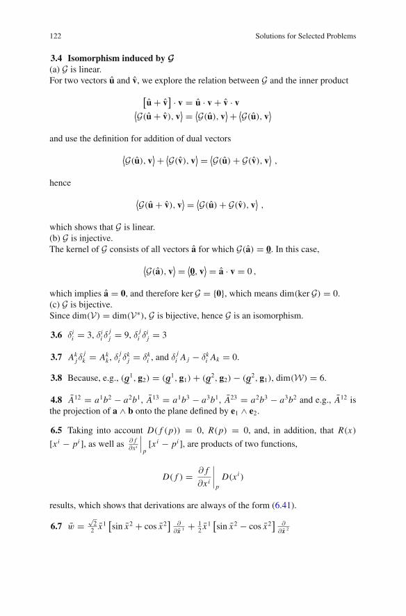
122 Solutions for Selected Problems
3.4 Isomorphism induced by G(a) G is linear.For two vectors u and v, we explore the relation between G and the inner product
[u + v
] · v = u · v + v · v⟨G(u + v), v
⟩ = ⟨G(u), v⟩ + ⟨G(u), v⟩
and use the definition for addition of dual vectors
⟨G(u), v⟩ + ⟨G(v), v⟩ = ⟨G(u) + G(v), v⟩ ,
hence
⟨G(u + v), v⟩ = ⟨G(u) + G(v), v⟩ ,
which shows that G is linear.(b) G is injective.The kernel of G consists of all vectors a for which G(a) = 0
˜. In this case,
⟨G(a), v⟩ = ⟨0˜, v
⟩ = a · v = 0 ,
which implies a = 0, and therefore ker G = {0}, which means dim(ker G) = 0.(c) G is bijective.Since dim(V) = dim(V∗), G is bijective, hence G is an isomorphism.
3.6 δii = 3, δii δjj = 9, δ j
i δij = 3
3.7 Akjδ
jk = Ak
k , δji δ
kj = δki , and δ
ji A j − δki Ak = 0.
3.8 Because, e.g., (g˜1, g2) = (g
˜1, g1) + (g
˜2, g2) − (g
˜2, g1), dim(W) = 6.
4.8 A12 = a1b2 − a2b1, A13 = a1b3 − a3b1, A23 = a2b3 − a3b2 and e.g., A12 isthe projection of a ∧ b onto the plane defined by e1 ∧ e2.
6.5 Taking into account D( f (p)) = 0, R(p) = 0, and, in addition, that R(x)
[xi − pi ], as well as ∂ f∂xi
∣∣∣p[xi − pi ], are products of two functions,
D( f ) = ∂ f
∂xi
∣∣∣∣p
D(xi )
results, which shows that derivations are always of the form (6.41).
6.7 w =√22 x1
[sin x2 + cos x2
]∂
∂ x 1 + 12 x
1[sin x2 − cos x2
]∂
∂ x 2

Index
Symbolsε-neighborhood, 11R, 28RN , 28
AAffine mapping, 77Affine space, 59Ambient space, 107Atlas, 103, 104
BBasis
vector space, 27change of, 30dual, 34orthonormal, 38, 74reciprocal, 34, 37
Basis isomorphism, 55, 65Bi-covector, 48Bi-vector, 48Bundle
fiber, 110tangent, 109
CCartesian coordinates, 66Cartesian product, 7Chain rule, 72Chart, 100, 103
affine, 77non-linear, 84
Christoffel-symbols, 92Commutative diagram, 7Compactness, 17, 18Connectedness, 17Connection, 92, 118Continuous mapping, 13Continuously differentiable, 70, 105Contraction, 46Coordinate chart, 16Coordinates
affine, 66, 79curvilinear, 89
Cross product, 49
DDerivation, 87, 108Derivative, 69
covariant, 90, 92Diffeomorphism, 104Differentiability, 73Differential form, 93Dimension
topological space, 17vector space, 26
Directional derivative, 71, 72, 81Distance function, 10, 14Div, 76Dual product, 34Dyadic product, 43
EEinstein-notation, 27, 29Embedding, 5, 109
© Springer International Publishing AG 2017U. Mühlich, Fundamentals of Tensor Calculus for Engineers with a Primeron Smooth Manifolds, Solid Mechanics and Its Applications 230,DOI 10.1007/978-3-319-56264-3
123

124 Index
Euclidean geometry, 1Euclidean space, 61Exterior derivative, 96Exterior product, 48, 53
FFiber bundle, 110Flow of a vector field, 114Force, 2, 35Form
alternating multi-linear, 48bilinear, 45differential, 93linear, 32multi-linear, 43, 45
Fréchet derivative, 73Function, 6
bounded, 18
GGateaux differential, 73Generalized Kronecker symbol, 51Global chart, 77Global vector balance, 5Grad, 76Gradient, 74Gradient operator, 76
HHausdorff, 19, 108Hodge-star-operator, 55Homeomorphism, 10, 16, 64Hybrid addition, 61
IIndex
lowering, 47raising, 47
Inner product, 35Integral curve, 114Integration, 93Interval
open, 15Isomorphism, 31
JJacobian, 80, 95
KKronecker symbol, 29
generalized, 51
LLagrangian description, 115Leibniz rule, 87, 107Lie bracket, 117Lie derivative, 114, 117Linear form, 32Linear mapping
image, 31kernel, 31rank, 31
Linearity, 32
MMöbius band, 110Manifold, 99
differentiable, 2smooth, 108topological, 108
Mapping, 6, 7affine, 62, 64, 77bijective, 7bilinear, 43continuous, 14, 15dual, 46injective, 7linear, 30surjective, 7
Metric, 11, 36coefficients, 38, 47
Motion, 17, 115
NNorm, 36
OOpen ε-ball, 11Open cover, 18Operator overloading, 25, 44Orientation, 95Oriented volume, 49
PParallel transport, 90, 92Parallelism, 1
absolute, 89

Index 125
Parametrization, 100Partial derivative, 74, 87Path, 17Path-connected, 17Permutation, 50Problems, 121Product
dual, 34dyadic, 43exterior, 48, 49, 53inner, 35
Product topology, 19Pull back, 79, 80, 86Push forward, 78, 80, 86
of vector fields, 83
RRank-nullity theorem, 31Reciprocal basis, 34, 37Rot, 76
SScalar field, 73Separability, 17Separable, 19Set
boundary, 12closed, 15interior, 11open , 14self-interior, 14
Skew-symmetric projection, 52Solutions, 121
Spaceaffine, 59dual, 34euclidean, 3metric, 10of polynomials PM , 28product space, 19tensor, 44topological, 15vector, 23
Stokes’ theorem, 95Subspace, 17
TTangent bundle, 109Tangent space, 87, 102, 103Tangent vector, 105
to curve, 82Tensor, 41
field, 73skew-symmetric, 50symmetric, 50
Topology, 3, 64basis, 19sub-basis, 20
Trajectory of a material point, 115Triangle inequality, 11, 12
VVector, 2
field, 73, 114linear independence, 26maximal set, 26