1

UWB Sparse/Diffuse Channels, Part I:Channel Models and Bayesian Estimators

Nicolò Michelusi, Student Member, IEEE, Urbashi Mitra, Fellow, IEEE, Andreas F. Molisch, Fellow, IEEE,and Michele Zorzi, Fellow, IEEE

Abstract—In this two-part paper, the problem of channelestimation in Ultra Wide-Band (UWB) systems is investigated.Due to the large transmission bandwidth, the channel has beentraditionally modeled as sparse. However, some propagationphenomena, e.g., scattering from rough surfaces and frequencydistortion, are better modeled by a diffuse channel. Herein, anovel Hybrid Sparse/Diffuse (HSD) channel model is proposed.Tailored to the HSD model, channel estimators are designed fordifferent scenarios that differ in the amount of side informationavailable at the receiver. An Expectation-Maximization algorithmto estimate the power delay profile of the diffuse componentis also designed. The proposed methods are compared to un-structured and purely sparse estimators. The numerical resultsshow that the HSD estimation schemes considerably improve theestimation accuracy and the bit error rate performance overconventional channel estimators. In Part II, the new channelestimators are evaluated with more realistic geometry-basedchannel emulators. The numerical results show that, even whenthe channel is generated in this manner, the new estimationstrategies achieve high performance. Moreover, a Mean-SquaredError analysis of the proposed estimators is performed, in thehigh and low Signal to Noise Ratio regimes, thus quantifying, inclosed form, the achievable performance gains.

Index Terms—Ultra Wideband, Bayesian estimation, channelestimation, channel modeling, sparse approximations

I. INTRODUCTION

Ultra Wide-Band (UWB) signaling had been originallyproposed as a technology for indoor mobile and multiple-access communications [1]–[3]. Due to its significant band-width, UWB offers high precision localization [4], robustnessagainst multipath fading [5] and immunity to narrow-bandinterference [6], thus representing a compelling solution forapplications such as short-range, high-speed broadband access[7], Wireless Body Area Networks (WBANs) [8], covertcommunication links, through-wall imaging, high-resolutionground-penetrating radar and asset tracking [9]–[11]. However,the performance of coherent UWB transceivers relies on theavailability of accurate channel estimates. Thus, it is importantto design channel estimation strategies that exploit the struc-tural and statistical properties of UWB propagation to achievethe best estimation accuracy.

Copyright (c) 2012 IEEE. Personal use of this material is permitted. How-ever, permission to use this material for any other purposes must be obtainedfrom the IEEE by sending a request to pubs-permissions@ieee.org.

N. Michelusi and M. Zorzi are with the Department ofInformation Engineering, University of Padova, Italy, e-mail:{michelusi,zorzi}@dei.unipd.it.

U. Mitra and A.F. Molisch are with the Ming Hsieh Department ofElectrical Engineering, University of Southern California, USA, e-mail:{ubli,molisch}@usc.edu.

The significant transmission bandwidth of UWB systemsenables a fine-grained delay resolution at the receiver, ofthe order of 1 ns. In many environments, only some ofthe resolvable delay bins carry significant multipath energy,yielding a sparse channel structure [10], [12]. For this reason,UWB channel estimation strategies based on compressivesensing and sparse approximation techniques [13]–[16] havebeen proposed in the literature, and they have been shownto outperform conventional unstructured estimators [17], [18].Also, localization techniques that exploit the information aboutthe specular multipath structure of the UWB channel have beenproposed (see, e.g., [19], [20]).

However, recent propagation studies suggest that, for someenvironments, such as indoor, WBANs and vehicular sce-narios, diffuse (dense) components of the impulse responsearise. These are caused by propagation processes such asdiffuse scattering [21], or unresolvable MultiPath Components(MPCs). Moreover, UWB channels exhibit a significant fre-quency dispersion [22] due to the large transmission bandwidthemployed. While irrelevant for conventional narrow-band sys-tems, this effect results in a pulse broadening and spreadingof the MPC energy over multiple resolvable delay bins. Thesepropagation mechanisms are not properly modeled by a purelysparse channel.

Recent work explores these effects. In [23], a geometry-based stochastic UWB model is proposed, consisting of astatistical model for the diffuse component. The model de-veloped in [24] combines a geometric approach to model theresolvable MPCs, and a stochastic approach to model thediffuse tail associated with each MPC. In [21], the spatialstructure of the diffuse MPCs is investigated, and its pa-rameters are extracted from the measurements. In [25], theimpact of diffuse scattering on the characteristics of vehicularpropagation channels in highway environments is evaluated,and the Doppler frequency-delay characteristics of diffusecomponents are analyzed. In [26], a low-complexity modelof diffuse scattering is proposed for vehicular radio channels.While these prior models were targeted towards performanceassessment, herein we develop a simplified UWB channelmodel suitable for channel estimation purposes and estimatoranalysis.

Exploitation of structure in channel models can lead toestimation strategies with strong performance, in [27], a Max-imum Likelihood (ML) estimator is designed which exploitsthe clustered structure of the UWB channel. In [28], a jointchannel estimation and decoding technique for Bit-InterleavedCoded Orthogonal Frequency Division Multiplexing is de-

2

signed, based on a two-state Gaussian mixture prior to modelthe sparse/diffuse structure of the channel, and on an hiddenMarkov prior to model clustering among the large taps.Therein, more structure is assumed, e.g., clustering of thetaps, and further the scheme is semi-blind. In [29], an MLframework is developed for parameter estimation in multi-dimensional channel sounding. Therein, the channel comprisesa deterministic component, resulting from specular reflection,and a stochastic component modeling diffuse scattering.

Our contributions are as follows: in Part I, based on theanalysis of the propagation mechanisms peculiar to UWBsystems, we present a novel Hybrid Sparse/Diffuse (HSD)UWB channel model [30]. In particular, we propose statisticalmodels for the sparse and diffuse components. We identifythree physically motivated scenarios that differ in the amountof side information available at the receiver (e.g., channel spar-sity level, Power Delay Profile (PDP) of the diffuse or sparsecomponent). For each scenario, Bayesian channel estimatorsare derived. In particular, we propose the Generalized MMSE(GMMSE) and the Generalized Thresholding (GThres) esti-mators, for the scenario where the statistics of the specularcoefficients are unknown. We also design an Expectation-Maximization (EM) algorithm for the PDP estimation of thediffuse component, which exploits the structure of the PDPover the channel delay dimension to enhance the estimationaccuracy.

The proposed algorithms are compared to unconstrainedestimators, which do not exploit the structure of the UWBchannel, and conventional sparse estimators, which, on theother hand, ignore the diffuse component of the channel. It isshown, by numerical results, that the new channel estimationmethods considerably improve the Mean-Squared Error (MSE)accuracy and the Bit Error Rate (BER) performance, thussuggesting the importance of a proper model for the UWBchannel. Specifically, a purely sparse estimator, by ignoring thediffuse component, is not able to capture important phenomenain UWB, e.g., pulse distortion [31] and diffuse scattering [22],thus failing to accurately estimate the channel. Moreover, it isshown that it is beneficial to be conservative in the estimationof the sparse component of the channel, by assuming that thesparse component is sparser than it actually is.

In Part II of this paper [32], we present an asymptoticMSE analysis of the GMMSE and the GThres estimators,in the regions of high and low Signal to Noise Ratios (SNR).Moreover, we validate the simplified HSD channel model andthe channel estimation strategies proposed in Part I, based ona realistic UWB channel model developed in [24]. We arguethat the HSD model, despite its simplicity, can effectivelycapture important UWB propagation mechanisms, such as finedelay resolution, scattering from rough surfaces and frequencydispersion. Moreover, due to its hybrid structure, the HSDmodel is robust and covers a wide range of practical scenarios,where the channel exhibits either a sparse, diffuse or hybridnature.

Part I of this paper is organized as follows: in Section II, weoverview the UWB propagation mechanisms. In Section III,we present the system model and the HSD channel model.In Section IV, we derive channel estimation strategies for the

HSD channel. In Section V, we present an EM algorithm forthe PDP estimation of the diffuse component. In Section VI,we provide simulation results and we compare the perfor-mance of the estimators. Finally, Section VII concludes thepaper.

Notation: We use lower-case bold letters for column vectors(a), and upper-case bold letters for matrices (A). The scalarak (or a(k)) denotes the kth entry of vector a, and Ak,j (orA(k, j)) denotes the (k, j)th entry of matrix A. A positivedefinite (positive semi-definite) matrix A is denoted by A � 0(A � 0). The transpose, complex conjugate of A is denotedby A∗. We define the square root of A � 0 with eigenvaluedecomposition A = UDU∗ as

√A = U

√DU∗. The

K × K unit matrix is defined as IK . The vector a � b isthe component-wise (Schur) product of vectors a and b. Theindicator function is given by I (·). We use p(·) to indicatea continuous or discrete probability distribution, and Pr (·)to indicate the probability of an event. The expectation ofrandom variable x, conditioned on y, is denoted by E [x|y].The Gaussian distribution with mean m and covariance Σis written as N (m,Σ), whereas the circularly symmetriccomplex Gaussian distribution is denoted by CN (m,Σ);1 theBernoulli distribution with parameter q is denoted by B(q).

II. UWB CHANNEL PROPAGATION AND MODELINGOVERVIEW

In this section, we overview the state of the art of UWBchannel propagation and modeling. The aim is to determinean appropriate UWB channel model, which captures the mainUWB propagation mechanisms. Neglecting pulse distortion[31] for simplicity, a time-varying channel in the continuoustime can be represented as [33]

h(τ, t) =∑l

al(t)δ(τ − τl(t)), (1)

where δ (·) is the Kronecker delta function, t is the timedimension and τ is the channel delay. The sum is over theMPCs, with time-varying amplitude al(t) and delay τl(t). Ifwe consider a UWB system with center frequency f0 andtransmission bandwidth W , the discrete baseband time-varyingimpulse response of the channel is given by

hbb(n, t) =∑l

al(t)e−i2πf0τl(t)sinc (n−Wτl(t)) , (2)

where sinc(x) = sin(πx)πx is the sinc function, and n ∈ Z

is the discrete channel delay. Due to the large transmissionbandwidth of UWB systems, MPCs arising from reflectionsand scattering in the environment spaced apart (in the delaydomain) by more than 1

W , which is typically of the orderof a fraction of a ns, can be resolved at the receiver. Then,by neglecting leakage effects due to the sampling of the sinc

1For a vector x = xR + ixI ∼ CN (0,Σ), where xR = Re(x),xI = Im(x) and i =

√−1, we define the covariance matrices of

its real and imaginary parts as E[xRx∗R] = E[xIx∗

I ] =Re(Σ)

2and

E[xIx∗R] = −E[xRx∗

I ] =Im(Σ)

2.

3

function off its peak, (2) is commonly approximated by thefollowing sparse discrete baseband representation:

hbb(n, t) '∑l

al(t)e−i2πf0τl(t)δ (n− rd (Wτl(t))) , (3)

where rd(x) returns the closest integer to x.However, in many practical scenarios of interest (e.g., indoor

environments), diffuse components, that cannot be describedby the above model, arise. These are created mainly by thefollowing phenomena: a large number of unresolved paths,diffuse scattering [22], pulse distortion resulting from the fre-quency dependence of the gain and efficiency of the antennasand of the dielectric or conductive materials, and diffractioneffects [31]. In [23], the following frequency response has beenproposed, modeling the contribution from all these effects:

HUWB(f) =

(SLOS(f) +

∑k

Sk(f) +D(f)

)f−m

F, (4)

where f is frequency. In particular, we recognize in SLOS(f)and

∑k Sk(f) the contributions from the line of sight and

the resolvable MPCs, respectively, i.e., the MPCs whose inter-arrival time is larger than 1

W , giving rise to a sparse componentin the time domain. The term D(f) represents the diffuse com-ponent due to multipath interference, and is associated withthe non-resolvable MPCs. Finally, f

−m

F models the frequencydistortion of the channel, where F is a normalization factorand m is the frequency decay exponent. Note that, in thismodel, the diffuse component is independent of the realizationof the discrete MPCs, while, in contrast, the work in [24]models the diffuse component as a diffuse tail associated witheach specular component.

It is worth noting that the level of channel diffuseness orsparseness depends primarily on two factors: the transmis-sion bandwidth and the environment. In fact, the larger thetransmission bandwidth, the finer the delay resolution at thereceiver, and the sparser the channel is expected to be. Onthe other hand, an environment with many scatterers or roughsurfaces, e.g., an indoor scenario or WBANs, is more likelyto give rise to a dense channel, due to the richer interactionamong the MPCs. Dense channels have been observed, e.g.,in gas stations [23], industrial [34], office [10] and vehicularenvironments [25]. We thus expect a dense or hybrid channelrepresentation to be relevant in these or similar scenarios.

Spatio-temporal scale of variation in the UWB channelWe now consider the spatio-temporal variation of the chan-

nel, due to the relative motion of the scatterers, receiver andtransmitter in the environment. For ease of exposition, weconsider movement of the receiver only. Ignoring Dopplereffects, which are left for future investigations, the channeltime-variations affect the amount of side-information availableat the receiver for the purpose of channel estimation, asdiscussed in Section III-B.

From the discrete baseband model (2), the phase2 varia-tion of the lth MPC over a time-interval ∆t is given by

2Note that "phase" is a narrow-band concept and can be used only as anapproximation in UWB systems, in particular when the lower band edge isat f = 0.

∆φl , 2π c0λ0|τl(t+ ∆t)− τl(t)|, where λ0 is the wavelength

at the center frequency, and c0 is the free space speed of light.Therefore, a significant phase variation (e.g., by more thanπ2 ) occurs when ∆φl >

π2 . This quantity corresponds, in the

spatial domain, to a wavelength or a fraction of it. Therefore,phase changes are expected to occur on a very small spatio-temporal scale.

Similarly, the variation of the MPC delay, over the sametime-interval ∆t, is given by ∆τl , |τl(t+ ∆t)− τl(t)|.Hence, a significant variation (e.g., by more than one channeldelay bin, 1

W ) occurs when ∆τl >1W , i.e., on a spatial scale

of c0W or roughly a number of wavelengths in the range [0.5, 5],

depending on the value of the transmission bandwidth W ,relative to the center frequency f0.

Finally, significant variations of the MPC amplitude al(t),due to shadowing effects, typically correspond to a spatialscale of several wavelengths.

Note that, due to mutual interference of the unresolvableMPCs contributing to the same tap location, changes in theamplitude of the diffuse components arise over the samespatio-temporal scale as the phase changes of the MPCs(small scale fading). On the other hand, the amplitude of theresolvable MPCs vary over a much larger spatio-temporal scale(large scale fading).

Remark 1. It is worth noting that the side-lobes of the sincfunction in (2) introduce faster time-variations of the amplitudeof the resolvable MPCs than the large-scale fading, over thesame spatio-temporal scale as the delay variations, and accountfor the leakage of the MPC energy over nearby channel taps.However, this phenomenon is limited, and can be quantifiedas follows. The most severe leakage occurs when the MPCarrives exactly in the middle between two sampling times,in which case most of the energy (2sinc(0.5)2 ' 80%) isspread equally between two nearby taps (each with amplitude1− sinc(0.5) ' 37% smaller than in the no leakage scenario,where the MPC delay is exactly an integer number of thesampling period), and the remaining 20% is leaked amongthe nearby taps. Therefore, the side-lobes of the sinc functionaccount for at most a 37% variation of the amplitude of themain MPC tap in (2). The problem of MPCs falling in betweentwo sample points can be modeled as a basis mismatch [35].

In the next section, we present the observation and thechannel models. In particular, in Section III-A we present theHSD model, which represents a simplification with respectto other models presented in the literature, e.g., (4), but atthe same time it captures the main propagation phenomenaof the UWB channel discussed in this section: resolvableMPCs, modeled by the sparse vector (3), unresolvable MPCs,diffuse scattering and frequency distortion, modeled by arandom, dense vector. Also, based on the analysis of the spatio-temporal scale of variation in the UWB channel, in SectionIII-B we discuss different practical scenarios, differing in theside-information available at the receiver for the purpose ofchannel estimation, which enables more accurate estimationtechniques.

4

III. SYSTEM MODEL

We consider a single-user UWB system. The source trans-mits a sequence of M = N +L− 1 pilot symbols, x(k), k =−(L − 1), . . . , N − 1, over a channel h(l), l = 0, . . . , L − 1with known delay spread L ≥ 1. The received, discrete time,baseband signal over the corresponding observation interval ofduration N is given by

y(k) =

L−1∑l=0

h(l)x(k − l) + w(k), k = 0, . . . , N − 1, (5)

where w(k) ∈ CN (0, σ2w) is i.i.d. noise.

If we collect the N received samples in the column vectory = [y(0), y(1), . . . , y(N − 1)]

T , we have the followingmatrix representation:

y = Xh + w. (6)

Above, X ∈ CN×L is the N × L Toeplitzmatrix associated with the pilot sequence, havingthe vector of the transmitted pilot sequence[x(−k), x(−k + 1), . . . , x(−k +N − 1)]

T, k = 0, . . . , L− 1,

as its kth column, h = [h(0), h(1), . . . , h(L− 1)]T ∈ CL

is the column vector of channel coefficients, andw = [w(0), w(1), . . . , w(N − 1)]

T ∼ CN (0, σ2wIN ) is

the noise vector.We assume X∗X � 0, so that the LS estimate hLS =

(X∗X)−1

X∗y is a sufficient statistic [36] for the channel.Therefore, without loss of generality for the purpose of chan-nel estimation, we consider the observation model

hLS =(X∗X)−1

X∗y=h+(X∗X)−1

X∗w=h+√

S−1

n, (7)

where we have defined the SNR matrix S = X∗Xσ2w� 0, and

n = 1σ2w

√S−1

X∗w ∼ CN (0, IL). With a slight abuse of no-tation, we will refer to the LS estimate hLS as the "observed"sequence. Moreover, we assume that the pilot sequence isorthogonal, so that S is a diagonal matrix. Then, the noisevector

√S−1

n in the LS estimate has independent entries. Thisassumption greatly simplifies the channel estimation problem.In fact, when the channel has independent entries over thedelay dimension (this is the case for the HSD model wedevelop), a per-tap estimation approach, rather than a jointone, is optimal. The case with non-orthogonal pilot sequencesis considered in Part II of the paper.

A. HSD Channel Model

The channel h follows the HSD model developed in [30],

h = as � cs + hd, (8)

where the terms as � cs ∈ CL and hd ∈ CL represent thesparse3 and the diffuse components, respectively.

In particular, as ∈ {0, 1}L is the sparsity pattern, which isequal to one in the positions of the specular MPCs, and equalto zero otherwise; its entries are drawn i.i.d. from B(q), where

3In the following, we use the terms sparse, specular and resolvable MPCsinterchangeably. In fact, the physical specular components (resolvable MPCs)of the channel can be modeled and represented by a sparse vector (3).

q � 1 so as to enforce sparsity. In the sequel, we refer to thenon-zero entries of as�cs ∈ CL as active sparse components.

The vector of sparse coefficients, cs ∈ CL, is drawn fromthe continuous probability distribution p(cs), with secondorder moment E [csc

∗s] = Λs, where Λs is a diagonal matrix

with entries given by the PDP Λs(k, k) = Ps(k), k =0, . . . , L− 1.4

Finally, we use the Rayleigh fading assumption for thediffuse component, hd ∼ CN (0,Λd), where Λd is diagonal,with entries given by the PDP Λd(k, k) = Pd(k), k =0, . . . , L− 1.

Remark 2. The Bernoulli model for as can be interpreted asa discretized Saleh-Valenzuela model [37]. In fact, accordingto the latter, the inter-arrival times of the specular componentshave an exponential distribution, whose discrete counterpart isthe geometric distribution. This in turn can be interpreted asthe inter-arrival time of two consecutive "1"s in a sequence ofi.i.d. Bernoulli draws.

Remark 3. In general, the Rayleigh fading assumption doesnot hold for the distribution of the sparse coefficients p(cs)(unlike the diffuse ones), since only very few propagationpaths contribute to an active tap in the sparse channel, thuslimiting the validity of the central limit theorem. Channelmeasurement campaigns have shown that the large scalefading, affecting the amplitude of the entries of cs, can bemodeled by a log-normal distribution [23]. However, for thesake of analytical tractability, in the following we either treatcs as a deterministic unknown vector, when its second ordermoment Λs is unknown, or we treat it using the Gaussianapproximation, when knowledge of Λs is available.

Remark 4. Note that in [23] the amplitudes of the diffusecoefficients are modeled by a Weibull distribution, with a delaydependent shape parameter σ < 2, and approach the Rayleighfading distribution (σ = 2) only for large excess delays. Thisdistribution represents a fading worse than Rayleigh. However,we adopt the Rayleigh fading approximation for simplicityand tractability. Also, the side-lobes of the sinc functionin (2) introduce correlation in the delay domain, which isnot accounted for under the Rayleigh fading model. This isa common assumption in standard cellular channel models,where measurements have well established the independenceof fading on different taps [38].

Despite its simplicity, we argue that the HSD model is ableto capture the main UWB propagation mechanisms discussedin Section II. In fact, the resolvable specular components andthe fine delay resolution are appropriately modeled by thesparse vector as � cs, whereas diffuse scattering, multipathinterference and the frequency distortion are approximated bythe diffuse component hd. This is confirmed by simulationresults in Part II of the paper, where we validate the proposedHSD model based on a realistic channel emulator [24].

4It is worth noting that this is not a PDP in the traditional sense, but ratherrepresents the power profile of the active sparse components, as a function ofthe delay.

5

B. Channel Estimation scenarios

The HSD model is described by a number of deterministicparameters, namely, the sparsity level q, the PDP of the diffusecomponent Pd and the PDP of the sparse component Ps.Accurate knowledge about some or all of these parametersmay not be available at the receiver, depending on a number offactors, most importantly the length of the interval over whichthe channel is observed, and the dynamics of the environment.

Let{

h(j) = a(j)s � c

(j)s + h

(j)d , j = 0, . . . , Nch − 1

}be a

sequence of Nch channel realizations, spaced apart in time by∆t, corresponding to a spatial separation by ' λ0, resultingfrom the relative motion of the receiver with respect to thescatterers and the transmitter position. Under this assumption,the samples of the diffuse component

{h

(j)d , j ≥ 0

}can be

approximated as drawn independently from CN (0,Λd), dueto multipath interference (Section II).

On the other hand, the positions of the active sparse co-efficients

{a

(j)s , j = 0, . . . , Nch − 1

}exhibit correlation with

each other. In fact, as pointed out in Section II, a variation ofthe delay associated with a specular MPC by one channel delaybin occurs over a spatial scale of the order of c0

Wλ0∈ [0.5, 5]

wavelengths. Therefore, the positions of the "1"s observed insubsequent realizations of the sparsity pattern a

(j)s are bound

not to vary appreciably over a large spatial scale, relative tothe wavelength.

A similar consideration holds for the amplitudes of thespecular components (i.e., the active sparse components in thevector a

(j)s � c

(j)s ), which vary according to the large scale

fading, i.e., over a relatively large spatial scale, compared tothe rate of variation of the diffuse component (however, theside-lobes of the sinc function account for a 37% variation inthe amplitude on the same spatial scale as the delay variations,as discussed in Remark 1 of Section II).

This correlation structure, i.e., slow amplitude and delayvariations, may be exploited to enhance the estimation ac-curacy of the sparse component a

(j)s � c

(j)s , by tracking the

position and amplitude of the resolvable MPCs over subse-quent observation windows. However, in this work we considerestimation of a

(j)s � c

(j)s based on either only one channel

realization, or the statistics of the ensemble of realizationsthat ignores the information about the temporal sequence inwhich the realizations occur.

We consider three different physical scenarios, dictated bythe length of the observation window Nch.

C. Single Snapshot of the channel

If a very short observation window is available (Nch = 1, orless than a wavelength in the spatial domain), averaging overthe small scale and the large scale fading is not possible. Un-der this assumption, statistical information about the channelcannot be reliably collected, and the channel can reasonably beconsidered a deterministic and unknown vector. In this case,an LS estimate hLS may be employed. In the absence of priorinformation about the channel, this is a robust approach forchannel estimation.

TABLE IESTIMATION SCENARIOS CONSIDERED.

Scenario sparsity q PDP Λs PDP Λd

S0 Single snapshot (unstructured) unknown unknown unknownS1 Single snapshot unknown unknown known

(PDP structure exploited)S2 Avg. over Small scale fading known unknown knownS3 Avg. over Small&Large scale fading known known known

Alternatively, we may exploit further structure of the chan-nel, e.g., exponential PDP of the diffuse component, to averagethe fading over the delay dimension rather than over time. Asshown in Section V, under this assumption, an accurate PDPestimate of h

(j)d is possible even in the extreme case Nch = 1.

We may then assume that the PDP of h(j)d is known at the

receiver, whereas the vector c(j)s is modeled as deterministic

and unknown.As to the sparsity level q, letting Nsc be the number of

resolvable scatterers, we have q ' Nsc

L . This number is notexpected to vary appreciably over a relatively long observationinterval, and can be estimated by counting the number ofresolvable MPCs which can be distinguished from the noiseplus diffuse background. However, an accurate estimate of Nsc

is obtained by averaging the small-scale fading and the noiseover subsequent channel realizations. Hence, we model q as adeterministic and unknown parameter.

D. Averaging over the Small scale fading

When a larger observation window is available (correspond-ing, in the spatial domain, to a few wavelengths, Nch > 1),averaging over the small scale fading (amplitude and phaseof the diffuse component) may be possible. In this case, thePDP of h

(j)d can be estimated accurately by averaging over

subsequent realizations of the fading process.In this scenario, we assume that Λd is perfectly known at

the receiver. This knowledge can be exploited by performinga Minimum MSE (MMSE) estimate of h

(j)d , which achieves

a better accuracy than LS. On the other hand, due to theinability to average over the large-scale fading, which affectsthe variation of the amplitude of the resolvable MPCs, c

(j)s is

treated as deterministic and unknown.

E. Averaging over the Small scale and the Large scale fading

Finally, when the observation interval spans several wave-lengths (Nch � 1), averaging over the large scale, other thanthe small scale fading, is possible.

In this scenario, we assume that Λd, Λs and q are knownat the receiver. This information can be exploited to computea linear-MMSE estimate of c

(j)s and h

(j)d , thus enhancing the

estimation accuracy over an unstructured estimate (e.g., LS).The main scenarios of interest, and the side information at

the receiver, are listed in Table I. Scenario S0 will not befurther considered, since the channel is estimated via LS. Inthe next section, we design channel estimators for the otherscenarios.

6

IV. HYBRID SPARSE/DIFFUSE CHANNEL ESTIMATION

In this section, we design channel estimation strategiesbased on the HSD model. In particular, for scenario S3, wepropose an MMSE estimator in Section IV-A. For scenariosS1 and S2, we propose the GMMSE and GThres estimatorsin Section IV-B.

A. MMSE Estimator

When Λd, Λs and q are known, we can devise an MMSE es-timator. By exploiting the orthogonality of the pilot sequence,we can use a per-tap estimation approach. The MMSE estimateof the kth delay bin is given by the posterior mean of thechannel, given the observed channel sample hLS(k) [36],

hMMSE(k)=Pr(as(k)=0|hLS(k))E [hd(k)|hLS(k),as(k)=0]

+ Pr(as(k)=1|hLS(k))E [cs(k) + hd(k)|hLS(k),as(k)=1] ,(9)

where we have conditioned on the realization of the sparsitybit as(k). In particular, the sum is over the posterior meanunder the two hypotheses as(k) = 1 and as(k) = 0,weighted by their posterior distribution Pr (as(k) = 1|hLS(k))and Pr (as(k) = 0|hLS(k)), respectively.

In order to compute (9), we use the circular Gaus-sian approximation for cs(k).5 Under this assumption,hLS(k)|{as(k) = a,h(k)} ∼ CN (h(k), 1/Sk,k), whereas thechannel sample h(k), conditioned on as(k) = a, is distributedas h(k)|as(k) = a ∼ CN (0,as(k)Ps(k) + Pd(k)). Then,h(k)|{hLS(k),as(k) = a} ∼ CN (m(a),Σ), with posteriormean m(a) = E [h(k)|hLS(k),as(k) = a] given by

m(a) =aPs(k) + Pd(k)

1/Sk,k + aPs(k) + Pd(k)hLS(k). (10)

From (9), we finally obtain

hMMSE(k) = Pr (as(k) = 0|hLS(k))Sk,kPd(k)

1 + Sk,kPd(k)hLS(k)

+ Pr (as(k) = 1|hLS(k))Sk,k (Ps(k) + Pd(k))

1 + Sk,k (Ps(k) + Pd(k))hLS(k),

where, from Bayes’ rule and as(k) ∼ B(q), lettingQk =

Sk,kPs(k)1+Sk,kPd(k) , we have

Pr (as(k) = 1|hLS(k))=

(1+

1− qq

p (hLS(k)|as(k) = 0)

p (hLS(k)|as(k) = 1)

)−1

=1

1 + 1−qq (1 + Qk) exp

{− Qk

1+Qk

Sk,k|hLS(k)|21+Sk,kPd(k)

} . (11)

5As discussed in Remark 3 in Section III, the large scale fading iscommonly modeled by a log-normal prior; however, due to the difficultyin handling it, the Rayleigh fading approximation is used, thus leading tothe classical linear MMSE estimator. We have numerically evaluated theperformance loss incurred by using the linear MMSE estimator over anMMSE estimator based on the log-normal prior, for the simple scalar modely = cs + n, where cs = eνs+iθs , with νs ∼ N (0, 1) and θs uniform in[0, 2π], is the channel coefficient with log-normal amplitude, n ∼ CN (0, σ2

w)is the noise; we found that the performance loss is at most 1.67 dB, at 0 dBSNR level.

B. Generalized MMSE (GMMSE) and Generalized Thresh-olding (GThres) Estimators

In this section, we develop estimators for scenarios S1 andS2. In particular, Λd is assumed to be known at the receiver,whereas cs is treated as a deterministic and unknown vector.The case where Λd is unknown and is estimated from theobserved sequence is treated in Section V.

For generality, we assume that the sparsity level q isunknown, and an estimate q of q, which might be differentfrom the real q, is used in the estimation phase. This choicerepresents a generalization with respect to [30], where thetrue sparsity level q is used. We will show by simulation, andby analysis in Part II of the paper, that assuming a sparsitylevel q < q often improves the estimation accuracy, thusimplying that knowledge of this parameter is not crucial tothe performance of the estimators.

We proceed as follows. cs is estimated by MaximumLikelihood (ML). Then, the estimate cs is used to performeither an MMSE or a Maximum A Posteriori (MAP) estimateof the sparsity pattern as, denoted by as, assuming the prioras ∼ B(q)L. We refer to these estimators as the GMMSEand GThres estimators, respectively. Finally, the diffuse com-ponent hd is estimated via MMSE, based on the residualestimation error hLS − as � cs.

The ML estimate of cs(k) is given by

cs(k) = arg mincs(k)∈C

{− ln p (hLS(k)|cs(k),as(k) = 1)}

= hLS(k), (12)

where we have used the fact that, when conditionedon as(k) = 0, the observation hLS(k) does notdepend on cs(k), and hLS(k)| {cs(k),as(k) = 1} ∼CN

(cs(k), [Sk,k]

−1+ Pd(k)

). We thus obtain cs = hLS.

Using the estimate cs(k) = hLS(k) and conditioning onas(k) = a, a ∈ {0, 1}, the MMSE estimate of the diffusecomponent hd(k) is given by

h(a)d (k) = E [hd(k)|hLS(k), cs(k), as(k) = a]

=Sk,kPd(k)

1 + Sk,kPd(k)(1− a) hLS(k). (13)

Finally, by combining the estimates as, cs and h(a)d , the

overall HSD estimate is given by

h(k)= as(k)hLS(k)+(1− as(k))Sk,kPd(k)

1+Sk,kPd(k)hLS(k). (14)

We now develop the MMSE and MAP estimates of as(k).1) Generalized MMSE Estimator:

The MMSE estimate of the sparsity bit as(k) is given by

a(GMMSE)s (k) = E [as(k)|hLS(k), cs(k)]

= Pr (as(k) = 1|hLS(k), cs(k)) . (15)

Using Bayes’ rule, cs(k) = hLS(k), and assuming as(k) ∼B(q), we have

a(GMMSE)s (k) =

1

1 + eα exp{−Sk,k|hLS(k)|2

1+Sk,kPd(k)

} , (16)

where we have defined α = ln(

1−qq

).

7

2) Generalized Thresholding Estimator:Using Bayes’ rule and the ML estimate cs(k) = hLS(k), theMAP estimate of as is given by

a(GThres)s (k) = arg max

a∈{0,1}{ln Pr (as(k) = a|hLS(k), cs(k))}

= arg mina∈{0,1}

{(1− a)

Sk,k |hLS(k)|2

1 + Sk,kPd(k)+ a ln

(1− qq

)}= I

(|hLS(k)|2 ≥ α (1/Sk,k + Pd(k))

). (17)

This solution consists in a thresholding of the LS estimate,hence the name Generalized Thresholding estimator, wherethe diffuse component represents noise for the estimationof the sparse coefficients. For this reason, the threshold isproportional, by a factor α, to the sum of the noise strength1/Sk,k and the power of the diffuse component Pd(k).

It is worth noting that, if α ≤ 0 (i.e., q ≥ 12 ), then

a(GThres)s (k) = 1, and the GThres estimator trivially reduces

to the LS solution.

V. STRUCTURED PDP ESTIMATION OF THE DIFFUSECOMPONENT

In the derivation of the GMMSE and GThres estimatorsin the previous section, we have assumed that the PDP ofthe diffuse component hd is perfectly known at the receiver.However, in a practical system, this is unknown, and thereforeneeds to be estimated.

Herein, we develop a structured estimate of the PDP Pd,when the observation interval is too short to allow time-averaging over the small scale fading. By exploiting priorinformation about the structure of the PDP, we can average thesmall scale fading over the delay dimension, rather than oversubsequent realizations of the fading process, thus enhancingthe estimation accuracy.

We assume an exponential PDP model [23], [38], [39]Pd(k) = βe−ωk, k = 0, . . . , L−1, where the deterministic,unknown parameters β ≥ 0 and ω ≥ 0 represent the relativepower and the decay rate of the PDP, respectively. We derivean ML estimate of these parameters, using the EM algorithm(the general EM framework is presented in, e.g., [40]). Forsimplicity, we assume a single channel snapshot. However, thefollowing derivation can be extended to include a sequence ofchannel realizations. Moreover, we treat the vector cs as adeterministic unknown parameter, and we assume a sparsitylevel q (possibly, 6= q), which is consistent with the designchoice of the GMMSE and GThres estimators.

Let the HSD channel and the observed sequence be givenby (8) and (7), respectively. From (8), if as(k) = 1, thenhLS(k) = cs(k) + hd(k) +

√Sk,k

−1n(k). In this case, since

cs(k) is a deterministic, unknown parameter, the observedsample hLS(k) does not provide statistical information toestimate the diffuse component (hence, its power). In fact, theML estimate of cs(k) is cs(k) = hLS(k) (12). The estimatedcontribution from the noise and the diffuse component is thenhLS(k)− cs(k) = 0, and the estimate of hd(k), given by (13),is forced to zero. Therefore, the observations correspondingto the active sparse components should be neglected in theestimation process.

Conversely, all the statistical information to estimate thePDP parameters ω and β is contained in the vector (1−as)�hLS = (1 − as) � (hd +

√S−1

n), which is obtained byzeroing the contribution from the active sparse components.Unfortunately, as is unknown in advance, hence it needs tobe estimated from the observed sequence.

In employing the EM algorithm to estimate the PDP pa-rameters β and ω, we assume as and (1 − as) � hd as thehidden variables. Moreover, we discard the contribution ofthe active sparse components to the observed sequence, asjustified above. Then, letting β, ω be the current estimates ofthe deterministic unknown parameters β and ω, respectively,in the E-step we compute (18), where, in the last step, we havedefined the posterior probability of an active sparse component

qpost(k) = Pr(as(k) = 1|hLS(k), β, ω, cs(k) = hLS(k)

)=

1

1 + 1−qq exp

{−Sk,k|hLS(k)|2

1+Sk,kβe−ωk

} . (19)

In particular, in step (a) we have expressed the likelihoodfunction in terms of its conditional probabilities. Moreover,we have used that fact that the term (1 − as) � hLS = (1 −as) � (hd +

√S−1

n) is independent of the PDP parametersβ, ω, when conditioned on (1−as)�hd and as, and the priordistribution of as is independent of β, ω. In step (b), we haveneglected the terms which are independent of the optimizationparameters β, ω. In step (c), the expectation is first conditionedon as = x, and then averaged over the posterior probabilityof as ∈ {0, 1}L. The conditional expectation of |hd(k)|2 isgiven by

E[|hd(k)|2

∣∣∣hLS(k),as(k) = 0, β, ω]

(20)

=Pd(k)2

(Pd(k) + 1/Sk,k)2|hLS(k)|2 +

Pd(k)

1 + Pd(k)Sk,k,

where Pd(k) = βe−ωk is the current estimate of the priorvariance of hd(k).

In the M-step, the term L(β, ω; β, ω) is minimized withrespect to the optimization parameters β, ω. We obtain{β, ω

}= arg minβ≥0,ω≥0

L(β, ω; β, ω) = arg minβ≥0,ω≥0

R(β, ω; β, ω)

= arg minβ≥0,ω≥0

L−1∑k=0

(1− qpost(k)) ln(βe−ωk

)(21)

+

L−1∑k=0

(1− qpost(k))E[|hd(k)|2

∣∣∣hLS(k),as(k) = 0, β, ω]

βe−ωk.

By defining, for k = 0, . . . , L− 1,Ak =

L(1−qpost(k))E[ |hd(k)|2|hLS(k),as(k)=0,β,ω]∑L−1p=0 (1−qpost(p))

,

Z =∑L−1

p=0 p(1−qpost(p))∑L−1p=0 (1−qpost(p))

,(22)

the M-step (21) is equivalent to{β, ω

}= arg min

β≥0,ω≥0lnβ − ωZ +

1

βL

L−1∑k=0

Akeωk. (23)

8

L(β, ω; β, ω) ,− E[

ln p ( (1− as)� hLS, (1− as)� hd,as|β, ω)|hLS, β, ω]

(18)

(a)= − E

[ln p ( (1− as)� hLS| (1− as)� hd,as)|hLS, β, ω

]− E

[ln p ( (1− as)� hd|as, β, ω)|hLS, β, ω

]− E

[ln p (as)|hLS, β, ω

](b)∝ −E

[ln p ( (1− as)� hd|as, β, ω)|hLS, β, ω

](c)= −

∑x∈{0,1}L

Pr(

as = x|hLS, β, ω, cs = hLS

)E[

ln p ( (1− as)� hd|as = x, β, ω)|hLS,as = x, β, ω]

=

L−1∑k=0

(1− qpost(k))

ln(βe−ωk

)+

E[|hd(k)|2

∣∣∣hLS(k),as(k) = 0, β, ω]

βe−ωk

, R(β, ω; β, ω)

We have the following theorem, whose proof is provided inthe Appendix.

Theorem 1. There is a unique solution{β, ω

}to

{β, ω

}= arg min

β≥0,ω≥0lnβ − ωZ +

1

βL

L−1∑k=0

Akeωk. (24)

If∑L−1k=0 (Z − k)Ak > 0, then ω is the unique solution in

(0,+∞) of

L−1∑k=0

(Z − k)Akeωk = 0. (25)

Otherwise, ω = 0. In both cases, β = 1L

∑L−1k=0 Ake

ωk.

Note that, when∑L−1k=0 (Z − k)Ak > 0, the solution is

a zero of a Lth order polynomial, therefore we must recurto approximate solutions. Since the solution we seek satisfiese−ω ∈ (0, 1], and we have proved that it is unique, we recurto the bisection method [41] to determine an approximate zerox = e−ω of (25).

Finally, the overall EM algorithm consists in the iterationsof the E-step (19), (22) and the M-step (23). The algorithmmay be initialized by neglecting the noise and the sparsecomponent, i.e., assuming Sk,k → +∞ and q = 0 in thefirst stage. In this case, we have qpost(k) = 0,∀k in (19) andthe parameters of the E-step (22) are given by

{Ak = |hLS(k)|2 , k = 0, . . . , L− 1Z = L−1

2 .(26)

It is worth noting that, if we had assumed the diffusecomponent hd, rather than (1−as)�hd, as the hidden variable,and we had used all the observed sequence hLS to estimatethe unknown PDP parameters instead of (1−as)�hLS, then

in the M-step we would have{β, ω

}= arg min

β≥0,ω≥0

L−1∑k=0

(1− qpost(k)) ln(βe−ωk

)(27)

+

L−1∑k=0

(1− qpost(k))E[|hd(k)|2

∣∣∣hLS(k),as(k) = 0, β, ω]

βe−ωk

+

L−1∑k=0

qpost(k)

ln(βe−ωk

)+

βe−ωk

βe−ωk(

1 + Sk,kβe−ωk) ,

where we have used the fact that, since cs = hLS,

E[|hd(k)|2

∣∣∣hLS(k), cs(k),as(k)=1, β, ω]=

βe−ωk

1 + Sk,kβe−ωk.

By comparing this expression with (21), we note one addi-tional term. In particular, the observations associated with highprobability qpost(k) → 1 with an active sparse componentgive a significant contribution to the log-likelihood function.However, these observations do not provide information aboutthe diffuse component hd, since cs is a deterministic, unknownvector. Conversely, in (21), these observations yield a negligi-ble contribution.

Choice of the sparsity level q

We next discuss the choice of the parameter q used toestimate the parameters β, ω. Since the EM algorithm solvesthe ML problem [40], we consider the general problem ofmaximizing the likelihood function. Assuming the sparsitylevel q, the ML estimate of β, ω and cs is defined as

{β, ω, cs} = arg maxβ≥0,ω≥0,cs

p(hLS|β, ω, cs)

= arg maxβ≥0,ω≥0,cs

−L−1∑k=0

ln (1/Sk,k + Pd(k))

+

L−1∑k=0

ln

(q exp

{−|hLS(k)− cs(k)|2

1/Sk,k + Pd(k)

}

+(1− q) exp

{− |hLS(k)|2

1/Sk,k + Pd(k)

}),

where we have used the fact that hLS(k)|as(k) = a ∼CN (acs(k),Pd(k) + 1/Sk,k) and Pd(k) = βe−ωk. By

9

maximizing over cs, we obtain cs = hLS. Then, lettingtk(Pd(k)) = |hLS(k)|2

1/Sk,k+Pd(k) , s(q, t) = ln(t+ 1−q

q te−t)

and

F(q, β, ω) =∑L−1k=0 s(q, tk(Pd(k))), we obtain

{β, ω}=arg maxβ≥0,ω≥0

L−1∑k=0

[ln tk(Pd(k))+ln

(1+

1− qq

e−tk(Pd(k))

)]

= arg maxβ≥0,ω≥0

L−1∑k=0

s(q, tk(Pd(k))) = arg maxβ≥0,ω≥0

F(q, β, ω),

where we have added the term∑L−1k=0 ln(|hLS(k)|2)− L ln q,

which does not affect the maximization.Consider a given pair of parameters (β, ω), and let

s′(q, t) ,ds(q, t)

dt=q − (1− q)e−t(t− 1)

qt+ (1− q)te−t, (28)

F ′β(q, β, ω) ,dF(q, β, ω)

dβ=

L−1∑k=0

s′(q, tk(Pd(k)))dtk(Pd(k))

dβ.

Similarly, we define F ′ω(q, β, ω) as the derivative with respectto ω. Note that, if F ′β(q, β, ω) > 0 (< 0), then there isan incentive to augment (diminish) β so as to increase thelog-likelihood function F(q, β, ω) (the same considerationholds for F ′ω(q, β, ω)). We now prove that this derivative is adecreasing function of q, so that, the larger q, the smaller theincentive to increase β (and, possibly, the larger the incentiveto decrease it, if the derivative becomes negative). In fact,

ds′(q, t)dq

=1

q2exp{−2s(q, t)}t2e−t > 0,

dtk(Pd(k))

dβ= − 1

βtk(Pd(k))

Pd(k)

1/Sk,k + Pd(k)< 0, (29)

and therefore

dF ′β(q, β, ω)

dq=

L−1∑k=0

ds′(q, tk(Pd(k)))

dq

dtk(Pd(k))

dβ< 0.

Similarly, we can prove that F ′ω(q, β, ω) is an increasingfunction of q, so that, the larger q, the smaller the incentive todecrease ω (and, possibly, the larger the incentive to increaseit, if the derivative becomes negative).

Moreover, note that, if q ≥ 11+e2 ' 0.12, then we have

e−t(t−1) ≤ e−2 ≤ q1−q (since the left hand side is maximized

for t = 2), which implies s′(q, t) ≥ 0,∀t. We conclude that,when q ≥ 1

1+e2 , the derivatives F ′β(q, β, ω) < 0, ∀β ≥ 0, ω ≥0 and F ′ω(q, β, ω) > 0, ∀β ≥ 0, ω ≥ 0. Therefore, the MLestimate of β, ω gives β = 0, ω → +∞, and the PDP estimateis forced to zero.

Conversely, if we let q → 0+, then the contribution of thesparse component as � cs is neglected, and the channel istreated as being purely diffuse.

This analysis proves that the prior sparsity level q ≥ 0.12should never be used, and suggests the existence of a trade-off in the optimal algorithm parameter q, which is confirmedby simulation in Section VI: in order not to force the PDPestimate to zero, q should be "small"; however, in orderto take into account the presence of the sparse componentin the observations, q should not be "too small". A furtherinvestigation on the optimal value of q is left for future work.

VI. SIMULATION RESULTS

In this section, we present the simulation results and eval-uate the MSE and BER performance achievable with theabove estimation strategies for a channel following the HSDmodel. In particular, the HSD model allows us to controlthe parameters (e.g., sparsity level q, PDP profiles Pd, Ps)and to evaluate the performance of the estimators developedin Section IV in an ideal setting, i.e., where the channelrealizations follow exactly the HSD model, based on whichthe estimators have been designed. Conversely, in Part II [32],simulation results are given based on a more realistic channelmodel [24], which allows us to evaluate the robustness of theproposed estimators against deviations from the HSD model.

We define the MSE of the estimator h of the channel h as

MSE =1

L

L−1∑k=0

E[∣∣∣h(k)− h(k)

∣∣∣2] . (30)

In the simulations, the channel h ∈ CL has delay spreadL = 100. The sparsity pattern as ∈ {0, 1}L has i.i.d. Bernoullientries with parameter q = 0.1. The vector cs ∈ CL isdrawn from CN (0,Λs), with exponential PDP Λs(k, k) =Ps(k) = Pse

−ωk, where ω = 0.05. The diffuse componenthd ∈ CL is drawn from CN (0,Λd), with exponential PDPΛd(k, k) = Pd(k) = βPse

−ωk. Unless otherwise stated, weuse β = 0.01, hence the ratio between the energy of the sparseand diffuse components is given by [E[h∗shs]/E[h∗dhd]] dB =10 dB, where hs = as � cs denotes the sparse compo-nent. The parameter Ps > 0 is a normalization factor, andis chosen so that the average channel energy is L, i.e.,∑L−1k=0 E

[|h(k)|2

]= Ps

∑L−1k=0 (β + q)e−ωk = L. We assume

an orthogonal pilot sequence, thus S is diagonal and can bedescribed as S = S · IL, where S > 0 is the estimation SNR.

We compare the LS estimate, the MMSE estimate (SectionIV-A), and the GMMSE and GThres estimators (SectionsIV-B1 and IV-B2, respectively), for different values of theassumed sparsity level q ∈ {0.1, 0.01, 0.001}, correspondingto α = 1−q

q ∈ {2.2, 4.6, 6.9}. We also compare theseestimators with a purely sparse and a purely diffuse estimators,which ignore the diffuse or sparse components, respectively.Since a per-tap approach is optimal in this case, for the sparseestimator we choose a variation of the GThres estimatorwhich assumes no diffuse component (hd = 0).

Note that the MMSE estimator in Section IV-A, by assum-ing perfect knowledge of q, Λd and Λs, is a lower bound tothe estimation accuracy. This is used primarily as a reference.

Figure 1 plots the MSE of the estimators, assuming perfectknowledge of Λd, as a function of the average SNR perchannel entry, defined as SE[h∗h]/L. We observe that, usinga more conservative approach, i.e., assuming a Bernoulli priorq � q, improves the estimation accuracy in the high andlow SNR regimes. In fact, the optimal threshold for theGThres estimator represents a balance between the proba-bility of mis-detecting an active sparse component as diffusecontribution and the probability of false alarm (detecting adiffuse contribution as active sparse component). A conser-vative approach, by employing a small threshold, reduces thefalse alarm probability (a similar consideration holds for the

10

−25 −20 −15 −10 −5 0 5 10 15 20 25

10−2

10−1

100

101

102

Estimation SNR, SE[h∗h]/L (dB)

MSE

LS

MMSE

GMMSE, q =0.1

GThres, q =0.1

GMMSE, q =0.01

GThres, q =0.01

GMMSE, q =0.001

GThres, q =0.001

Diffuse, q = 0

Fig. 1. MSE of the channel estimators, assuming perfect knowledge of thePDP Pd(k). β = 0.01, q = 0.1

GMMSE estimator). This trend can also be observed in themedium SNR ranges. However, this property does not hold ingeneral. To see that, we also plot the accuracy of the diffuseestimator h(Diff)(k) = SPd(k)

1+SPd(k)hLS(k), which ignores thesparse component as � cs. This can be interpreted as a limitcase of the GMMSE and GThres estimators, for q → 0,or equivalently α → +∞. An analytical explanation of thisbehavior, based on the MSE analysis of the estimators in theasymptotic regimes of high and low SNR, follows in Part II ofthis paper [32]. Note also that the GMMSE estimator performsbetter than the GThres estimator with respect to MSE, fora given value of q. This is a consequence of the fact thatGThres allows only the extreme values a

(GThres)s (k) ∈ {0, 1},

whereas GMMSE allows a smoother transition between thesetwo extremes.

In Figure 2, we let vary the ratio between the energies ofthe sparse and diffuse components,E[h∗shs]/E[h∗dhd] = q/β. The SNR per channel entry is[SE[h∗h]/L] dB = 10 dB. The MSE of the purely sparseestimator is also plotted in this case. Similarly to Figure 1,we note that a conservative approach is beneficial from anMSE perspective. As expected, the sparse estimator performsworse than the GThres estimator, due to its inability toexploit the diffuse component of the channel. In particular, itperforms closely to the GThres estimator for small values ofβ (i.e., large values of E[h∗shs]/E[h∗dhd]), where the diffusecomponent is negligible with respect to the sparse one, andincurs a performance degradation for large values of β, wherethe diffuse component becomes significant. Moreover, as ex-pected, the only diffuse estimator achieves good performancefor large values of β. However, it performs poorly for smallvalues of β, where the sparse component yields a significantcontribution. Note that, excluding the MMSE estimator, theGThres estimator with q = 0.001 achieves the best perfor-mance over the entire range of values considered, very closeto the MMSE lower bound. This proves that the proposedmethods are robust, and adapt to a wide range of estimationscenarios, where the channel exhibits either a sparse, diffuseor hybrid nature (corresponding to large, small and moderate

−10 −5 0 5 10 15 20 25 30 3510

−2

10−1

100

Sparse/Diffuse ratio, E[h∗shs]/E[h∗

dhd] (dB)

MSE

LS

MMSE

GThres, q =0.1

Sparse, q =0.1

GThres, q =0.001

Sparse, q =0.001

Diffuse

Fig. 2. MSE of the channel estimators as a function of β, assuming perfectknowledge of the PDP of the diffuse component Pd(k). [SE[h∗h]/L] dB =10dB, q = 0.1

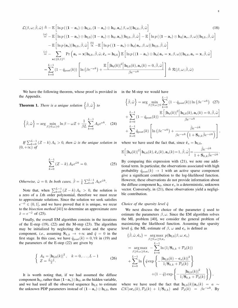
values of E[h∗shs]/E[h∗dhd], respectively).Figure 3 compares the MSE of the GMMSE estimator, for

the two cases where Λd is perfectly known at the receiver,and where it is estimated from the observed sequence usingthe EM algorithm (Section V), based on only one realizationof the channel. We notice that, in general, there is a smallperformance loss due to the unknown Λd, mainly in the lowSNR range and for small values of q (however, no performancedegradation is observed for q = 0.1). This behavior isexplained by the fact that the MMSE estimate of hd in (14) ismore sensitive to errors in the estimation of Λd in the low SNRthan in the high SNR regime. In fact, for high SNR values,it approaches the LS solution. On the other hand, for smallvalues of q we have the following. The posterior probabilityof the entries of the sparsity pattern as, as a function of thefactor α =

(1−qq

), is given by (16) with Sk,k = S. This

is a decreasing function of α (i.e., increasing function of q).As a consequence, the smaller q the more the weight givento the right-hand term of (14), associated with the MMSEestimate of hd(k), which is sensitive to errors in the estimateof Pd(k), compared to the left-hand term, associated withthe LS estimate of cs(k), which is independent of the PDPestimate. As a consequence, a smaller value of q results inan overall estimate that is more sensitive to errors in the PDPestimate of hd. Similar considerations hold for the GThresestimator.

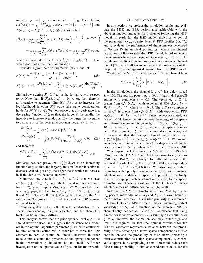
Figure 4 plots the MSE of PDP estimator of the diffusecomponent developed in Section V, for different values of qand of the number of iterations of the EM algorithm, basedon only one channel realization, as a function of the SNRper diffuse channel entry SE[h∗dhd]/L. In particular, lettingPd(k), k = 0, . . . , L − 1 be an estimate of Pd(k) = βe−ωk,we compute the following MSE metric:

MSEPDP =1

L

L−1∑k=0

E[(

ln Pd(k)− lnPd(k))2]. (31)

The performance is compared also with an oracle estimator,which assumes perfect knowledge of as�cs, thus being able to

11

−25 −20 −15 −10 −5 0 5 10 1510

−2

10−1

100

101

102

Estimation SNR, SE[h∗h]/L (dB)

MSE

LS

MMSE

GMMSE, q =0.1

GMMSE, q =0.1, PDP.est.

Sparse, q =0.1

GMMSE, q =0.001

GMMSE, q =0.001, PDP.est.

Sparse, q =0.001

Fig. 3. MSE of the GMMSE estimators, comparison between the caseswhere the PDP of the diffuse component is known and estimated from thedata, respectively. β = 0.01, q = 0.1. The two curves of the GMMSEestimator with q = 0.1 where the PDP is known and estimated overlap.

perfectly remove the interference from the sparse component(in particular, we use the EM estimator with q = 0). In theFigure, the MSE floor refers to the ML estimator of β, ω inthe noiseless scenario with no sparse component. It can beshown that, in this case, the ML estimator is obtained bysetting Ak = |hd(k)|2 and Z = L−1

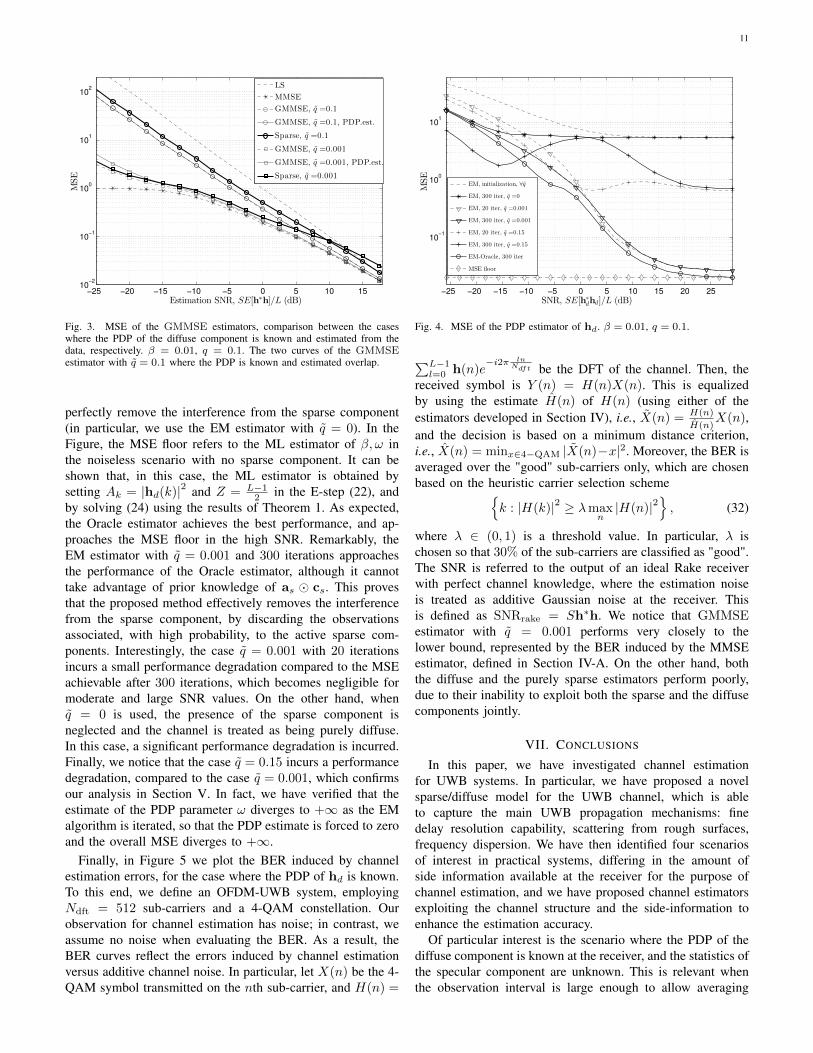
2 in the E-step (22), andby solving (24) using the results of Theorem 1. As expected,the Oracle estimator achieves the best performance, and ap-proaches the MSE floor in the high SNR. Remarkably, theEM estimator with q = 0.001 and 300 iterations approachesthe performance of the Oracle estimator, although it cannottake advantage of prior knowledge of as � cs. This provesthat the proposed method effectively removes the interferencefrom the sparse component, by discarding the observationsassociated, with high probability, to the active sparse com-ponents. Interestingly, the case q = 0.001 with 20 iterationsincurs a small performance degradation compared to the MSEachievable after 300 iterations, which becomes negligible formoderate and large SNR values. On the other hand, whenq = 0 is used, the presence of the sparse component isneglected and the channel is treated as being purely diffuse.In this case, a significant performance degradation is incurred.Finally, we notice that the case q = 0.15 incurs a performancedegradation, compared to the case q = 0.001, which confirmsour analysis in Section V. In fact, we have verified that theestimate of the PDP parameter ω diverges to +∞ as the EMalgorithm is iterated, so that the PDP estimate is forced to zeroand the overall MSE diverges to +∞.

Finally, in Figure 5 we plot the BER induced by channelestimation errors, for the case where the PDP of hd is known.To this end, we define an OFDM-UWB system, employingNdft = 512 sub-carriers and a 4-QAM constellation. Ourobservation for channel estimation has noise; in contrast, weassume no noise when evaluating the BER. As a result, theBER curves reflect the errors induced by channel estimationversus additive channel noise. In particular, let X(n) be the 4-QAM symbol transmitted on the nth sub-carrier, and H(n) =

−25 −20 −15 −10 −5 0 5 10 15 20 25

10−1

100

101

SNR, SE[h∗

dhd]/L (dB)

MSE

EM, initialization, ∀q

EM, 300 iter, q =0

EM, 20 iter, q =0.001

EM, 300 iter, q =0.001

EM, 20 iter, q =0.15

EM, 300 iter, q =0.15

EM-Oracle, 300 iter

MSE floor

Fig. 4. MSE of the PDP estimator of hd. β = 0.01, q = 0.1.

∑L−1l=0 h(n)e

−i2π lnNdft be the DFT of the channel. Then, the

received symbol is Y (n) = H(n)X(n). This is equalizedby using the estimate H(n) of H(n) (using either of theestimators developed in Section IV), i.e., X(n) = H(n)

H(n)X(n),

and the decision is based on a minimum distance criterion,i.e., X(n) = minx∈4−QAM |X(n)−x|2. Moreover, the BER isaveraged over the "good" sub-carriers only, which are chosenbased on the heuristic carrier selection scheme{

k : |H(k)|2 ≥ λmaxn|H(n)|2

}, (32)

where λ ∈ (0, 1) is a threshold value. In particular, λ ischosen so that 30% of the sub-carriers are classified as "good".The SNR is referred to the output of an ideal Rake receiverwith perfect channel knowledge, where the estimation noiseis treated as additive Gaussian noise at the receiver. Thisis defined as SNRrake = Sh∗h. We notice that GMMSEestimator with q = 0.001 performs very closely to thelower bound, represented by the BER induced by the MMSEestimator, defined in Section IV-A. On the other hand, boththe diffuse and the purely sparse estimators perform poorly,due to their inability to exploit both the sparse and the diffusecomponents jointly.

VII. CONCLUSIONS

In this paper, we have investigated channel estimationfor UWB systems. In particular, we have proposed a novelsparse/diffuse model for the UWB channel, which is ableto capture the main UWB propagation mechanisms: finedelay resolution capability, scattering from rough surfaces,frequency dispersion. We have then identified four scenariosof interest in practical systems, differing in the amount ofside information available at the receiver for the purpose ofchannel estimation, and we have proposed channel estimatorsexploiting the channel structure and the side-information toenhance the estimation accuracy.

Of particular interest is the scenario where the PDP of thediffuse component is known at the receiver, and the statistics ofthe specular component are unknown. This is relevant whenthe observation interval is large enough to allow averaging

12

0 5 10 15 20 25 30 35

10−6

10−5

10−4

10−3

10−2

10−1

Effective SNR, SE[h∗h] (dB)

BER,4-QAM

LS

MMSE

GMMSE, q =0.001

Sparse, q =0.001

Diffuse, q = 0

Fig. 5. BER induced by channel estimation errors, with known PDP of hd.β = 0.01, q = 0.1.

over the small scale fading, but not over the large scalefading. For this scenario, we have proposed the GeneralizedMMSE and Generalized Thresholding Estimators. Moreover,we have proposed an EM algorithm for the PDP estimationof the diffuse component, which exploits the exponentialstructure of the PDP to average the fading over the channeldelay dimension, rather than over subsequent independentrealizations of the fading process.

We have compared these estimators to the unconstrained LSestimator, and to conventional purely sparse or diffuse estima-tors, which, on the other hand, ignore either the diffuse or thesparse component. The numerical results show that, when thechannel follows the hybrid sparse/diffuse model, the proposedestimators considerably improve the performance over LS andconventional sparse or diffuse estimators, from both an MSEand a BER perspective. Moreover, we have observed that it isbeneficial to be conservative in the estimation of the sparsecomponent of the channel, i.e., to assume that the sparsecomponent is sparser than it actually is. In Part II, we developan MSE analysis of these estimators, proving this conjecturein the asymptotic high and low SNR regimes, and we validatethe proposed sparse/diffuse model and estimation strategiesbased on a more realistic UWB channel emulator.

ACKNOWLEDGMENTS

This research has been funded in part by the followinggrants and organizations: ONR N00014-09-1-0700, NSF CNS-0832186, NSF CNS-0821750 (MRI), Aldo Gini Foundation(Padova, Italy).

APPENDIX

Proof of Theorem 1 in Section V. Let f(x, β) = lnβ +Z lnx + 1

βL

∑L−1k=0 Akx

−k, where we have defined x =

e−ω ∈ (0, 1] in the argument of the minimization in (24).By minimizing with respect to β ≥ 0, for a fixed x, we have

β(x) = arg minβ≥0

{lnβ +

1

βL

L−1∑k=0

Akx−k}

=1

L

L−1∑k=0

Akx−k.

Substituting into f(x, β), we obtain f(x, β(x)) = 1+ln β(x)+Z lnx. We now minimize f(x, β(x)) with respect to x ∈(0, 1]. f(x, β(x)) is an increasing function of x ∈ (0, 1] ifand only if

f ′(x, β(x)) =df(x, β(x))

dx=β′(x)

β(x)+Z

x> 0, (33)

where β′(x) = dβ(x)dx = − 1

L

∑L−1k=0 kAkx

−(k+1). Equiva-lently, multiplying both sides by xZ+1β(x) > 0, f(x, β(x))is an increasing function of x ∈ (0, 1] if and only if

g(x) , xZ+1β(x)f ′(x, β(x)) (34)

=1

L

L−1∑k=0

AkxZ−k (Z − k) > 0.

Note that g′(x) = dg(x)dx = 1

L

∑L−1k=0 Akx

Z−k−1 (Z − k)2>

0, ∀x ∈ (0, 1]. Therefore, g(x) is a continue monotoneincreasing function of x. Moreover, since Z < L − 1 from(22) and limx→0+ xm = +∞ when m < 0, we havelimx→0+ g(x) = −∞. Therefore, if g(1) > 0, or equivalently∑L−1k=0 (Z − k)Ak > 0, then there exists a unique x ∈ (0, 1)

solution of g(x) = 0 such that{g(x) > 0, ∀x > xg(x) < 0, ∀x < x.

(35)

Equivalently, x ∈ (0, 1) is the unique solution off ′(x, β(x)) = 0 such that{

f ′(x, β(x)) > 0, ∀x > x

f ′(x, β(x)) < 0, ∀x < x.(36)

As a consequence, x is the unique minimizer of f(x), x ∈(0, 1], and

{β(x), ω = − ln x

}uniquely minimizes (24).

Conversely, if g(1) ≤ 0, i.e.,∑L−1k=0 (Z − k)Ak ≤ 0, then

g(x) ≤ 0, ∀x ∈ (0, 1]. This is equivalent to f ′(x, β(x)) ≤0, ∀x ∈ (0, 1]. As a consequence, 1 is the unique minimizerof f(x, β(x)), and

{β(1), ω = 0

}uniquely minimizes (24).

REFERENCES

[1] M. Win and R. Scholtz, “Impulse radio: how it works,” IEEE Commu-nications Letters, vol. 2, no. 2, pp. 36–38, Feb. 1998.

[2] R. Scholtz, “Multiple access with time-hopping impulse modulation,”in IEEE Military Communications Conference, vol. 2, Oct. 1993, pp.447–450.

[3] R. Qiu, H. Liu, and X. Shen, “Ultra-wideband for multiple accesscommunications,” IEEE Communications Magazine, vol. 43, no. 2, pp.80–87, Feb. 2005.

[4] S. Gezici, Z. Tian, G. Giannakis, H. Kobayashi, A. Molisch, H. Poor,and Z. Sahinoglu, “Localization via Ultra-Wideband radios: a look atpositioning aspects for future sensor networks,” IEEE Signal ProcessingMagazine, vol. 22, no. 4, pp. 70–84, July 2005.

[5] M. Win and R. Scholtz, “On the robustness of ultra-wide bandwidth sig-nals in dense multipath environments,” IEEE Communications Letters,vol. 2, no. 2, pp. 51–53, Feb. 1998.

[6] M. Chiani and A. Giorgetti, “Coexistence Between UWB and Narrow-Band Wireless Communication Systems,” Proceedings of the IEEE,vol. 97, no. 2, pp. 231–254, Feb. 2009.

[7] A. Batra, J. Balakrishnan, G. Aiello, J. Foerster, and A. Dabak, “Designof a multiband OFDM system for realistic UWB channel environments,”IEEE Transactions on Microwave Theory and Techniques, vol. 52, no. 9,Sep. 2004.

13

[8] T. Zasowski, G. Meyer, F. Althaus, and A. Wittneben, “Propagationeffects in UWB body area networks,” in IEEE International Conferenceon Ultra-Wideband (ICU), Sep. 2005, pp. 16–21.

[9] L. Yang and G. Giannakis, “Ultra-Wideband Communications: an ideawhose time has come,” IEEE Signal Processing Magazine, vol. 21, no. 6,pp. 26–54, Nov. 2004.

[10] A. Molisch, D. Cassioli, C.-C. Chong, S. Emami, A. Fort, B. Kannan,J. Karedal, J. Kunisch, H. Schantz, K. Siwiak, and M. Win, “A Compre-hensive Standardized Model for Ultrawideband Propagation Channels,”IEEE Transactions on Antennas and Propagation, vol. 54, no. 11, pp.3151–3166, Nov. 2006.

[11] G. Aiello and G. Rogerson, “Ultra-Wideband Wireless Systems,” IEEEMicrowave Magazine, vol. 4, no. 2, June 2003.

[12] A. Molisch, “Ultra-Wide-Band Propagation Channels,” Proceedings ofthe IEEE, vol. 97, no. 2, pp. 353–371, Feb. 2009.

[13] T. Blumensath and M. Davies, “Iterative Thresholding for Sparse Ap-proximations,” Journal of Fourier Analysis and Applications, vol. 14,pp. 629–654, 2008, 10.1007/s00041-008-9035-z.

[14] S. S. Chen, D. L. Donoho, and M. A. Saunders, “Atomic Decompositionby Basis Pursuit,” SIAM Review, vol. 43, no. 1, pp. 129–159, 2001.

[15] R. Tibshirani, “Regression shrinkage and selection via the lasso,” Jour-nal of the Royal Statistical Society. Series B (Methodological), vol. 58,no. 1, pp. 267–288, 1996.

[16] W. Bajwa, J. Haupt, A. Sayeed, and R. Nowak, “Compressed ChannelSensing: A New Approach to Estimating Sparse Multipath Channels,”Proceedings of the IEEE, vol. 98, no. 6, pp. 1058–1076, June 2010.

[17] C. Carbonelli, S. Vedantam, and U. Mitra, “Sparse Channel Estimationwith Zero Tap Detection,” IEEE Transactions on Wireless Communica-tions, vol. 6, no. 5, pp. 1743–1763, May 2007.

[18] J. Paredes, G. Arce, and Z. Wang, “Ultra-Wideband Compressed Sens-ing: Channel Estimation,” IEEE Journal of Selected Topics in SignalProcessing, vol. 1, no. 3, pp. 383–395, Oct. 2007.

[19] P. Meissner, T. Gigl, and K. Witrisal, “UWB sequential Monte Carlopositioning using virtual anchors,” in International Conference on IndoorPositioning and Indoor Navigation (IPIN), Sep. 2010, pp. 1–10.

[20] Y. Shen and M. Win, “Fundamental Limits of Wideband Localization-Part I: A General Framework,” IEEE Transactions on InformationTheory, vol. 56, no. 10, pp. 4956–4980, Oct. 2010.

[21] F. Quitin, C. Oestges, F. Horlin, and P. De Doncker, “Diffuse multipathcomponent characterization for indoor MIMO channels,” in Proceedingsof the Fourth European Conference on Antennas and Propagation(EuCAP), Apr. 2010, pp. 1–5.

[22] A. Molisch, “Ultrawideband propagation channels-Theory, Measure-ment, and Modeling,” IEEE Transactions on Vehicular Technology,vol. 54, no. 5, pp. 1528–1545, Sep. 2005.

[23] T. Santos, F. Tufvesson, and A. Molisch, “Modeling the Ultra-WidebandOutdoor Channel: Model Specification and Validation,” IEEE Transac-tions on Wireless Communications, vol. 9, no. 6, pp. 1987–97, June2010.

[24] J. Kunisch and J. Pamp, “An ultra-wideband space-variant multipathindoor radio channel model,” in IEEE Conference on Ultra WidebandSystems and Technologies, Nov. 2003, pp. 290–294.

[25] Y. Zhou, X. Yin, N. Czink, T. Zemen, A. Guo, and F. Liu, “Evaluationof Doppler-Delay Properties of Diffuse Components in Vehicular Prop-agation Channels,” in 2nd IEEE International Conference on WirelessAccess in Vehicular Environments, Dec. 2009.

[26] N. Czink, F. Kaltenberger, Y. Zhou, L. Bernado, T. Zemen, and X. Yin,“Low-Complexity Geometry-Based Modeling of Diffuse Scattering,”in Proceedings of the Fourth European Conference on Antennas andPropagation (EuCAP), Apr. 2010.

[27] C. Carbonelli and U. Mitra, “Clustered ML Channel Estimation forUltra-Wideband Signals,” IEEE Transactions on Wireless Communica-tions, vol. 6, no. 7, pp. 2412–2416, July 2007.

[28] P. Schniter, “A Message-Passing Receiver for BICM-OFDM Over Un-known Clustered-Sparse Channels,” IEEE Journal of Selected Topics inSignal Processing, vol. 5, no. 8, pp. 1462–1474, Dec. 2011.

[29] R. Thoma, M. Landmann, and A. Richter, “RIMAX-a Maximum Likeli-hood Framework for Parameter Estimation in Multidimensional ChannelSounding,” in International Symposium on Antennas and Propagation(ISAP), Aug. 2004.

[30] N. Michelusi, U. Mitra, and M. Zorzi, “Hybrid Sparse/Diffuse UWBchannel estimation,” in IEEE 12th International Workshop on SignalProcessing Advances in Wireless Communications (SPAWC), June 2011,pp. 201–205.

[31] R. Qiu, “A study of the ultra-wideband wireless propagation channeland optimum UWB receiver design,” IEEE Journal on Selected Areasin Communications, vol. 20, no. 9, pp. 1628–1637, Dec. 2002.

[32] N. Michelusi, U. Mitra, A. Molisch, and M. Zorzi, “UWB Sparse/DiffuseChannels, Part II: Estimator Analysis and Practical Channels,” IEEETransactions on Signal Processing, 2012, to be published.

[33] A. Molisch, Wireless Communications, Second Edition, ser. Wiley-IEEE.John Wiley & Sons, 2011.

[34] J. Karedal, S. Wyne, P. Almers, F. Tufvesson, and A. Molisch, “Statisti-cal analysis of the UWB channel in an industrial environment,” in IEEE60th Vehicular Technology Conference, vol. 1, Sep. 2004, pp. 81–85.

[35] Y. Chi, L. Scharf, A. Pezeshki, and A. Calderbank, “Sensitivity toBasis Mismatch in Compressed Sensing,” IEEE Transactions on SignalProcessing, vol. 59, no. 5, pp. 2182–2195, May 2011.

[36] E. L. Lehmann and G. Casella, Theory of Point Estimation, 2nd ed.Springer, Aug. 1998.

[37] A. Saleh and R. Valenzuela, “A Statistical Model for Indoor MultipathPropagation,” Journal on Selected Areas in Communications, vol. 5,no. 2, pp. 128–137, Feb. 1987.

[38] D. Cassioli, M. Win, and A. Molisch, “The ultra-wide bandwidthindoor channel: from statistical model to simulations,” IEEE Journalon Selected Areas in Communications, vol. 20, no. 6, pp. 1247–1257,Aug. 2002.

[39] J. Hansen, “An analytical calculation of power delay profile and delayspread with experimental verification,” IEEE Communications Letters,vol. 7, no. 6, pp. 257–259, June 2003.

[40] A. P. Dempster, N. M. Laird, and D. B. Rubin, “Maximum likelihoodfrom incomplete data via the EM algorithm,” Journal of the RoyalStatistical Society. Series B (Methodological), vol. 39, 1977.

[41] R. L. Burden and J. D. Faires, Numerical Analysis, 9th Edition. CengageLearning, 2011.

14

Nicolò Michelusi (S’09) received the B.S. (Elec-tronics Engineering) and M.S. (TelecommunicationsEngineering) degrees summa cum laude from theUniversity of Padova, Italy, in 2006 and 2009, re-spectively, and the M.S. degree in Telecommuni-cations Engineering from Technical University ofDenmark, Copenhagen, Denmark, in 2009, as part ofthe T.I.M.E. double degree program. Since January2009, he is a Ph.D. student at University of Padova,Italy. In 2011, he was on leave at the Universityof Southern California, Los Angeles, United States,

as a visiting Ph.D. student. His research interests include ultrawidebandcommunications, wireless networks, cognitive networks, optimal control,energy harvesting for communications.

Urbashi Mitra received the B.S. and the M.S. degrees from the Universityof California at Berkeley and her Ph.D. from Princeton University. After asix year stint at the Ohio State University, she joined the Department ofElectrical Engineering at the University of Southern California, Los Angeles,where she is currently a Professor. Dr. Mitra has been an Associate Editor forthe following IEEE publications: Transactions on Information Theory (2007-2011), Journal of Oceanic Engineering (2006-2011), and Transactions onCommunications (1996-2001). She was a member of the IEEE InformationTheory Society’s Board of Governors (2002-2007) and began a third termin 2012. Dr. Mitra is also a member of the IEEE Signal Processing Soci-ety’s Technical Committee on Signal Processing for Communications andNetworking (2012-2014). She is the recipient of: 2012 NAE Lillian GilbrethLectureship, 2011 USC Zumberge Interdisciplinary Innovation Fund (with M.El-Naggar), USC Center for Excellence in Research Fellowship (2010-2013),the Viterbi School of Engineering Dean’s Faculty Service Award (2009), USCMellon Mentoring Award (2008), IEEE Fellow (2007), Texas InstrumentsVisiting Professor (Fall 2002, Rice University), 2001 Okawa FoundationAward, 2000 Lumley Award for Research (OSU College of Engineering),1997 MacQuigg Award for Teaching (OSU College of Engineering), and a1996 National Science Foundation (NSF) CAREER Award. Dr. Mitra hasheld visiting appointments at: the Delft University of Technology, StanfordUniversity, Rice University, and the Eurecom Institute. She served as co-Director of the Communication Sciences Institute at the University of SouthernCalifornia from 2004-2007.

Andreas F. Molisch (S’89-M’95-SM’00-F’05) re-ceived the Dipl. Ing., Ph.D., and habilitation degreesfrom the Technical University of Vienna, Vienna,Austria, in 1990, 1994, and 1999, respectively. Hesubsequently was with AT&T (Bell) LaboratoriesResearch (USA); Lund University, Lund, Sweden,and Mitsubishi Electric Research Labs (USA). Heis now a Professor of electrical engineering with theUniversity of Southern California, Los Angeles. Hiscurrent research interests are the measurement andmodeling of mobile radio channels, ultra-wideband

communications and localization, cooperative communications, multiple-input-multiple-output systems, and wireless systems for healthcare. He hasauthored, coauthored, or edited four books (among them the textbook WirelessCommunications, Wiley-IEEE Press), 14 book chapters, some 140 journalpapers, and numerous conference contributions, as well as more than 70patents and 60 standards contributions. Dr. Molisch has been an Editor ofa number of journals and special issues, General Chair, Technical ProgramCommittee Chair, or Symposium Chair of multiple international conferences,as well as Chairman of various international standardization groups. He isa Fellow of the IET, an IEEE Distinguished Lecturer, and a member ofthe Austrian Academy of Sciences. He has received numerous awards, mostrecently the 2011 James Evans Avant-Garde award of the IEEE VehicularTechnology Society, the Donald Fink Prize of the IEEE, and the Eric SumnerAward of the IEEE.

Michele Zorzi (S’89, M’95, SM’98, F’07) was bornin Venice, Italy, on December 6th, 1966. He receivedthe Laurea and the PhD degrees in Electrical En-gineering from the University of Padova, Italy, in1990 and 1994, respectively. During the AcademicYear 1992/93, he was on leave at the University ofCalifornia, San Diego (UCSD) as a visiting PhDstudent, working on multiple access in mobile radionetworks. In 1993, he joined the faculty of the Dipar-timento di Elettronica e Informazione, Politecnicodi Milano, Italy. After spending three years with

the Center for Wireless Communications at UCSD, in 1998 he joined theSchool of Engineering of the University of Ferrara, Italy, where he became aProfessor in 2000. Since November 2003, he has been on the faculty at theInformation Engineering Department of the University of Padova. His presentresearch interests include performance evaluation in mobile communicationssystems, random access in mobile radio networks, ad hoc and sensor networks,energy constrained communications protocols, broadband wireless access andunderwater acoustic communications and networking.

Dr. Zorzi was the Editor-In-Chief of the IEEE WIRELESS COMMU-NICATIONS MAGAZINE from 2003 to 2005 and the Editor-In-Chief ofthe IEEE TRANSACTIONS ON COMMUNICATIONS from 2008 to 2011,and currently serves on the Editorial Board of the WILEY JOURNAL OFWIRELESS COMMUNICATIONS AND MOBILE COMPUTING. He wasalso guest editor for special issues in the IEEE PERSONAL COMMUNI-CATIONS MAGAZINE (Energy Management in Personal CommunicationsSystems) IEEE WIRELESS COMMUNICATIONS MAGAZINE (CognitiveWireless Networks) and the IEEE JOURNAL ON SELECTED AREASIN COMMUNICATIONS (Multi-media Network Radios, and UnderwaterWireless Communications Networks). He served as a Member-at-large of theBoard of Governors of the IEEE Communications Society from 2009 to 2011.