UvA-DARE is a service provided by the library of the University of Amsterdam (http://dare.uva.nl)

UvA-DARE (Digital Academic Repository)

Comparing supernova remnants around strongly magnetized and canonical pulsars

Martin, J.; Rea, N.; Torres, D.F.; Papitto, A.

Published in:Monthly Notices of the Royal Astronomical Society

DOI:10.1093/mnras/stu1594

Link to publication

Citation for published version (APA):Martin, J., Rea, N., Torres, D. F., & Papitto, A. (2014). Comparing supernova remnants around stronglymagnetized and canonical pulsars. Monthly Notices of the Royal Astronomical Society, 444(3), 2910-2924. DOI:10.1093/mnras/stu1594

General rightsIt is not permitted to download or to forward/distribute the text or part of it without the consent of the author(s) and/or copyright holder(s),other than for strictly personal, individual use, unless the work is under an open content license (like Creative Commons).

Disclaimer/Complaints regulationsIf you believe that digital publication of certain material infringes any of your rights or (privacy) interests, please let the Library know, statingyour reasons. In case of a legitimate complaint, the Library will make the material inaccessible and/or remove it from the website. Please Askthe Library: http://uba.uva.nl/en/contact, or a letter to: Library of the University of Amsterdam, Secretariat, Singel 425, 1012 WP Amsterdam,The Netherlands. You will be contacted as soon as possible.

Download date: 18 Jun 2018

MNRAS 444, 2910–2924 (2014) doi:10.1093/mnras/stu1594

Comparing supernova remnants around strongly magnetized andcanonical pulsars

J. Martin,1‹ N. Rea,1,2 D. F. Torres1,3 and A. Papitto1

1Institute of Space Sciences (CSIC–IEEC), Faculty of Science, Campus UAB, Torre C5-parell, E-08193 Barcelona, Spain2Anton Pannekoek Institute for Astronomy, University of Amsterdam, Postbus 94249, NL-1090 GE Amsterdam, the Netherlands3Institucio Catalana de Recerca i Estudis Avanats (ICREA), E-08010 Barcelona, Spain

Accepted 2014 August 4. Received 2014 August 2; in original form 2014 April 9

ABSTRACTThe origin of the strong magnetic fields measured in magnetars is one of the main uncertaintiesin the neutron star field. On the other hand, the recent discovery of a large number of suchstrongly magnetized neutron stars is calling for more investigation on their formation. The firstproposed model for the formation of such strong magnetic fields in magnetars was throughalpha-dynamo effects on the rapidly rotating core of a massive star. Other scenarios involvehighly magnetic massive progenitors that conserve their strong magnetic moment into the coreafter the explosion, or a common envelope phase of a massive binary system. In this work, wedo a complete re-analysis of the archival X-ray emission of the supernova remnants (SNRs)surrounding magnetars, and compare our results with all other bright X-ray emitting SNRs,which are associated with compact central objects (which are proposed to have magnetar-likeB-fields buried in the crust by strong accretion soon after their formation), high-B pulsars andnormal pulsars. We find that emission lines in SNRs hosting highly magnetic neutron starsdo not differ significantly in elements or ionization state from those observed in other SNRs,neither averaging on the whole remnants, nor studying different parts of their total spatialextent. Furthermore, we find no significant evidence that the total X-ray luminosities of SNRshosting magnetars, are on average larger than that of typical young X-ray SNRs. Althoughbiased by a small number of objects, we found that for a similar age, there is the samepercentage of magnetars showing a detectable SNR than for the normal pulsar population.

Key words: line: identification – stars: magnetars – pulsars: general – ISM: supernovaremnants – X-rays: general.

1 IN T RO D U C T I O N

Supernova (SN) explosions are among the most energetic and ex-treme events ever observed in the Universe. Supernovae (SNe) aremainly distinguished in two main classes: core-collapse (CC) andthermonuclear SNe. CCSNe result from the core collapse of a mas-sive star (>8 M�; see Woosley & Janka 2005, for a review), whilethermonuclear SNe are due to the explosion of a white dwarf in abinary system with a giant star (single-degenerate origin), or fromtwo low-mass white dwarfs in a binary system (double-degenerateorigin; Hillebrandt & Niemeyer 2000). CCSNe might leave be-hind a fast rotating (several milliseconds) and strongly magnetized(>1012 G) stellar core which is now made by degenerate matter:a so-called neutron star. At the same time, the envelope of themassive star, ejected at high speed (∼104 km s−1) into the interstel-

� E-mail: martin@ieec.uab.es

lar medium (ISM), interacts with it, resulting in what is called asupernova remnant (SNR). In the standard picture, an SNR evolvesin time following four main expansion phases: free expansion,Sedov–Taylor phase, radiative and merging phase. The time-scalesand properties of each of those phases are characterized by the ini-tial SN explosion energy, interstellar ambient density, and the ageof the remnant (see Vink 2012 for a recent review).

In the recent years, a class of highly magnetized neutron stars(a.k.a. magnetars) have been discovered. Magnetars are a smallgroup of X-ray pulsars (about 20 objects with spin periods between2 and 12 s), the emission of which is not explained by the commonscenario for pulsars. In fact, the very strong X-ray emission of theseobjects (Lx ∼ 1035 erg) seemed too high and variable to be fed bythe rotational energy alone (as in the radio pulsars), and no evidencefor a companion star has been found in favour of any accretion pro-cess (see Mereghetti 2008 and Rea & Esposito 2011 for reviews).Assuming the typical magnetic loss equation for rotating neutronstars, their inferred magnetic fields appear to be in general of the

C© 2014 The AuthorsPublished by Oxford University Press on behalf of the Royal Astronomical Society

Comparing SNRs around PSRs 2911

order of B ∼ 1014–1015 G (although low magnetic field magnetarshave been recently discovered; Rea et al. 2010, 2012). Becauseof these high-B fields, the emission of magnetars is thought to bepowered by the decay and the instability of their strong fields (Dun-can & Thompson 1992; Thompson & Duncan 1993; Thompson,Lyutikov & Kulkarni 2002).

The exact mechanism playing a key role in the formation of suchstrong magnetic fields is currently debated; in particular, it is notclear which are the characteristics of a massive star turning into a‘magnetar’ instead of a normal radio pulsar, after its SN explosion.

Preliminary calculations have shown that the effects of a turbu-lent dynamo amplification occurring in a newly born neutron starcan indeed result in a magnetic field of a few 1017 G. This dynamoeffect is expected to operate only in the first ∼10 s after the SNexplosion of the massive progenitor, and if the protoneutron star isborn with sufficiently small rotational periods (of the order of a fewms). The resulting amplified magnetic fields are expected to havea strong multipolar structure, and toroidal component (Duncan &Thompson 1992, 1996; Thompson & Duncan 1993). However, thisscenario is encountering more and more difficulties: (i) if magnetictorques can indeed remove angular momentum from the core viathe coupling to the atmosphere in a pre-SN phase, then the coresoon after the SN might not spin rapidly enough for this convectivedynamo mechanism to take place (Heger, Woosley & Spruit 2005);(ii) such a fast spinning protoneutron star would require a SN ex-plosion one order of magnitude more energetic than normal SNe,possibly a hypernova, which is not yet clear whether it can indeedform a neutron star instead of a black hole. Recent simulationshave shown that gamma ray bursts (GRBs) and hyperluminous SNecan indeed be powered by recently formed millisecond magnetars(Metzger et al. 2011; Bucciantini et al. 2012), although no observa-tional evidence of the existence of such fast spinning and stronglymagnetized neutron stars have been collected thus far.

Besides the fast spinning protoneutron star, a further idea onthe origin of these high magnetic fields is that they simply reflectthe high magnetic field of their progenitor stars. Magnetic fluxconservation (Woltjer 1964) implies that magnetars must then be thestellar remnants of stars with internal magnetic fields of B > 1 kG,whereas normal radio pulsars must be the end products of lessmagnetic massive stars.

Recent theoretical studies showed that there is a wide spreadin white dwarf progenitor magnetic fields (Wickramasinghe &Ferrario 2005), which, when extrapolated to the more massiveprogenitors, implies a similar wide spread in neutron star pro-genitors (Ferrario & Wickramasinghe 2006). Hence, apparently itseems that a fossil magnetic field might be the solution of the ori-gin of such strongly magnetized neutron stars, without the needof invoking dynamo actions on utterly fast spinning protoneutronstars.

However, this lead to the problem of the formation of such high-Bprogenitor stars. The most common idea is that the magnetic field inthe star reflects the magnetic field of the cloud from which the staris formed. The best studied very massive stars (around ∼40 M�)with a directly measured magnetic field are θ Orion C and HD191612, with dipolar magnetic field of 1.1 and 1.5 kG, respec-tively (Donati et al. 2002, 2006). Very interestingly, the magneticfluxes of both these stars (1.1 × 1027 G cm2 for θ Orion C and7.5 × 1027 G cm2 for HD 191612) are comparable to the flux of thehighest field magnetar SGR 1806−20 (5.7 × 1027 G cm2; Woods &Thompson 2006). Other high magnetic field stars are reported inOskinova et al. (2011).

Recent observations of the environment of some magnetars re-vealed strong evidence that these objects are formed from the ex-plosion of very massive progenitors (M > 30 M�). In particular:(i) a shell of H I has been detected around 1E 1048.1−5937, and in-terpreted as ISM displaced by the wind of a progenitor of 30–40 M�(Gaensler et al. 2005); (ii) SGR 1806−20 and SGR 1900+14 havebeen claimed to be hosted by very young and massive star clus-ters, providing a limit on their progenitor mass of >50 M� (Fuchset al. 1999; Figer et al. 2005; Davies et al. 2009) and >20 M� (Vrbaet al. 2000), respectively. Finally, CXOU 010043−7211 is a mem-ber of the massive cluster Westerlund 1 (Muno et al. 2006; Ritchieet al. 2010), with a progenitor with mass estimated to be >40 M�(see also Clark et al. 2014).

Vink & Kuiper (2006) have started the idea of studying the ener-getics of SNRs surrounding magnetar with the aim of disentanglinga possible energetic difference between those remnants and otherssurrounding normal pulsars. Their work did not find any clear evi-dence, i.e. of an additional energy released in the remnant possiblydue to an excess of rotational energy at birth.

Following this study, we decided to extend their work re-analysing all available XMM–Newton or Chandra data of allconfirmed and bright SNRs associated with a magnetar or with ahigh-B pulsar showing magnetar-like activity, and comparing ina coherent and comprehensive way all the extracted properties ofthese SNRs with other remnants: in particular, line ionization andX-ray luminosity. In Section 2, we report on the data analysis andreduction of our observational sample, in Section 3 the results ofour analysis, and we discuss our findings in Section 4.

2 DATA A NA LY S I S A N D R E D U C T I O N

In this work, our approach has tried to be as conservative andmodel independent as possible. In particular, our target sample hasbeen chosen such so as to include all confirmed associations (seethe McGill catalogue1 for all proposed associations), and amongthose, we chose only SNRs bright enough, and with sufficientlygood spectra, to perform a detailed analysis and classification oftheir spectral lines. We analyse the X-ray spectral lines of fourSNRs hosting a neutron star that showed magnetar-like activity inits centre: Kes 73, CTB 109, N 49 and Kes 75 (see Fig. 1). Weuse for all targets the best available archival data: from the XMM–Newton telescope in the case of Kes 73, CTB 109 and N 49, andChandra for Kes 75. The observations used are summarized inTable 1. To compare coherently all the spectral lines and fluxes weobserved for these remnants, we have chosen to use an empiricalspectral fitting for all SNRs. We have modelled all spectra usingone or two Bremsstrahlung models for the spectral continuum, plusGaussian functions for each detected spectral line. We added spec-tral lines one by one until the addition of a further line did notsignificantly improve the fit (by using the F-test). This approachis totally empirical, with respect to using more detailed ionizedplasma models, but ensures a coherent comparison between differ-ent remnants. In Table 2, we report also the results of our spectramodelled with ionized plasma models, for a comparison with theliterature.

1 http://www.physics.mcgill.ca/pulsar/magnetar/main.html

MNRAS 444, 2910–2924 (2014)

2912 J. Martin et al.

Figure 1. Combined colour images of Kes 73 (top left), CTB 109 (top right), N 49 (bottom left) and Kes 75 (bottom right).

Table 1. Observations used in this paper.

SNR Instrument ObsID Date Detector Exp. (s)

Kes 73 XMM 0013340101 2002-10-05 PN 6017MOS1 5773MOS2 5771

0013340201 2002-10-07 PN 6613MOS1 6372MOS2 6372

CTB 109 XMM 0057540101 2002-01-22 PN 12 237MOS1 19 027MOS2 19 026

0057540201 2002-07-09 PN 14 298MOS1 17 679MOS2 17 679

0057540301 2002-07-09 PN 14 011MOS1 17 379MOS2 17 379

N 49 XMM 0505310101 2007-11-10 PN 72 172Kes 75 Chandra 748 2000-10-15 ACIS-S 37 280

6686 2006-06-07 ACIS-S 54 0707337 2006-06-05 ACIS-S 17 3607338 2006-06-09 ACIS-S 39 2507339 2006-06-12 ACIS-S 44 110

2.1 XMM–Newton data

We use images in full-frame mode obtained from the EuropeanPhoton Imaging Camera (EPIC) PN (Struder et al. 2001) and MOS(Turner et al. 2001). The spectra of these images are fitted simulta-neously in order to obtain the spectrum with the maximum possiblenumber of counts. We used the specific software for XMM–Newtondata, Science Analysis System (SAS) v13.5.0 with the latest cali-bration files. To clean images of solar flares, we used the SAS tooltabtigen to choose the good time intervals and extract them andthe spectra with evselect. Source and background spectra were ex-tracted from each single image with pattern ≤4 for PN images andpattern ≤12 for MOS. The spectra and the backgrounds correspond-ing to the same regions and the same detector were merged usingthe FTOOLS routine mathpha and we compute the mean of the re-sponse matrices (RMF) and the ancillary files (ARF) weighted bythe exposure time using the tools addrmf and addarf (this meansthat we keep PN, MOS1 and MOS2 data separately and we mergethe spectra when they come from the same detector). Finally, webinned the spectra demanding a minimum of 25 counts per bin toallow the use of χ2-statistics.

We analyse the spectrum of each nebula considering its entireextension. For Kes 73, the nebula is completely covered in the

MNRAS 444, 2910–2924 (2014)

Comparing SNRs around PSRs 2913

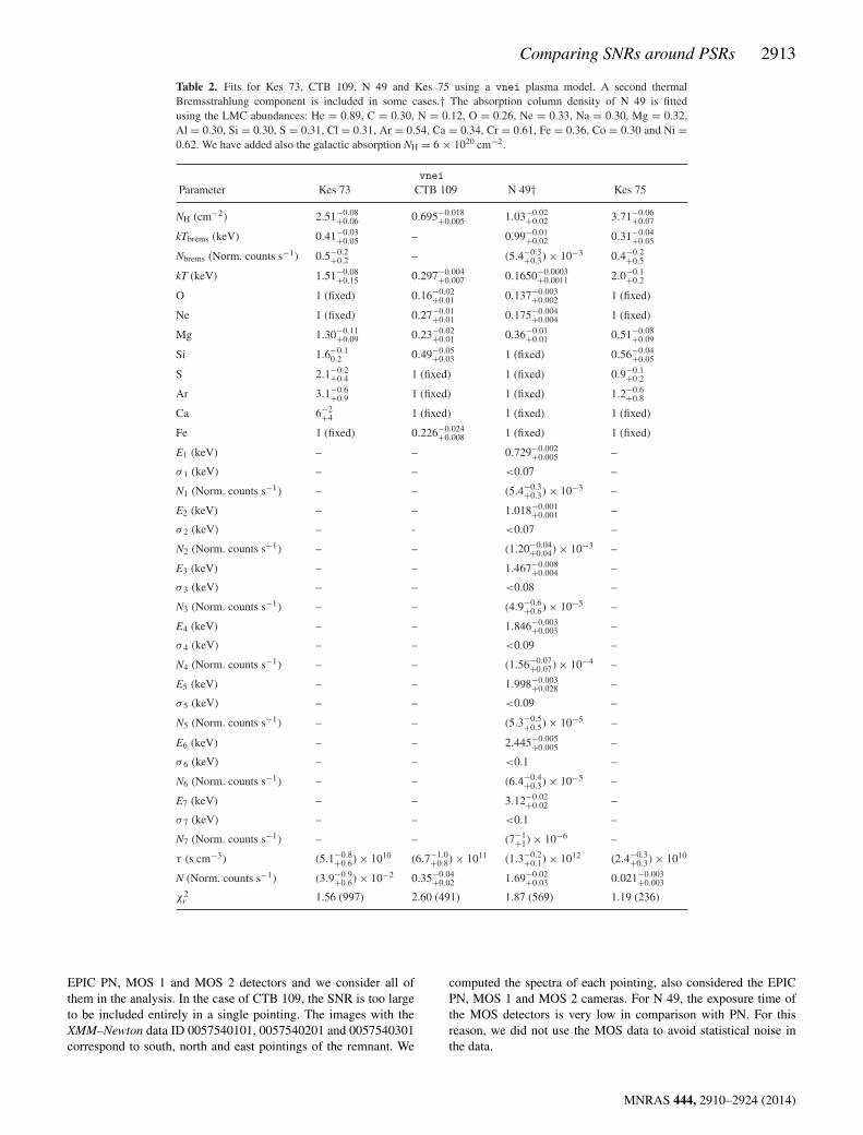
Table 2. Fits for Kes 73, CTB 109, N 49 and Kes 75 using a vnei plasma model. A second thermalBremsstrahlung component is included in some cases.† The absorption column density of N 49 is fittedusing the LMC abundances: He = 0.89, C = 0.30, N = 0.12, O = 0.26, Ne = 0.33, Na = 0.30, Mg = 0.32,Al = 0.30, Si = 0.30, S = 0.31, Cl = 0.31, Ar = 0.54, Ca = 0.34, Cr = 0.61, Fe = 0.36, Co = 0.30 and Ni =0.62. We have added also the galactic absorption NH = 6 × 1020 cm−2.

vnei

Parameter Kes 73 CTB 109 N 49† Kes 75

NH (cm−2) 2.51−0.08+0.06 0.695−0.018

+0.005 1.03−0.02+0.02 3.71−0.06

+0.07

kTbrems (keV) 0.41−0.03+0.05 – 0.99−0.01

+0.02 0.31−0.04+0.05

Nbrems (Norm. counts s−1) 0.5−0.2+0.2 – (5.4−0.3

+0.3) × 10−3 0.4−0.2+0.5

kT (keV) 1.51−0.08+0.15 0.297−0.004

+0.007 0.1650−0.0003+0.0011 2.0−0.1

+0.2

O 1 (fixed) 0.16−0.02+0.01 0.137−0.003

+0.002 1 (fixed)

Ne 1 (fixed) 0.27−0.01+0.01 0.175−0.004

+0.004 1 (fixed)

Mg 1.30−0.11+0.09 0.23−0.02

+0.01 0.36−0.01+0.01 0.51−0.08

+0.09

Si 1.6−0.10.2 0.49−0.05

+0.03 1 (fixed) 0.56−0.04+0.05

S 2.1−0.2+0.4 1 (fixed) 1 (fixed) 0.9−0.1

+0.2

Ar 3.1−0.6+0.9 1 (fixed) 1 (fixed) 1.2−0.6

+0.8

Ca 6−2+4 1 (fixed) 1 (fixed) 1 (fixed)

Fe 1 (fixed) 0.226−0.024+0.008 1 (fixed) 1 (fixed)

E1 (keV) – – 0.729−0.002+0.005 –

σ 1 (keV) – – <0.07 –

N1 (Norm. counts s−1) – – (5.4−0.3+0.3) × 10−3 –

E2 (keV) – – 1.018−0.001+0.001 –

σ 2 (keV) – - <0.07 –

N2 (Norm. counts s−1) – – (1.20−0.04+0.04) × 10−3 –

E3 (keV) – – 1.467−0.008+0.004 –

σ 3 (keV) – – <0.08 –

N3 (Norm. counts s−1) – – (4.9−0.6+0.6) × 10−5 –

E4 (keV) – – 1.846−0.003+0.003 –

σ 4 (keV) – – <0.09 –

N4 (Norm. counts s−1) – – (1.56−0.07+0.07) × 10−4 –

E5 (keV) – – 1.998−0.003+0.028 –

σ 5 (keV) – – <0.09 –

N5 (Norm. counts s−1) – – (5.3−0.5+0.5) × 10−5 –

E6 (keV) – – 2.445−0.005+0.005 –

σ 6 (keV) – – <0.1 –

N6 (Norm. counts s−1) – – (6.4−0.4+0.3) × 10−5 –

E7 (keV) – – 3.12−0.02+0.02 –

σ 7 (keV) – – <0.1 –

N7 (Norm. counts s−1) – – (7−1+1) × 10−6 –

τ (s cm−3) (5.1−0.8+0.6) × 1010 (6.7−1.0

+0.8) × 1011 (1.3−0.2+0.1) × 1012 (2.4−0.3

+0.3) × 1010

N (Norm. counts s−1) (3.9−0.9+0.6) × 10−2 0.35−0.04

+0.02 1.69−0.02+0.03 0.021−0.003

+0.003

χ2r 1.56 (997) 2.60 (491) 1.87 (569) 1.19 (236)

EPIC PN, MOS 1 and MOS 2 detectors and we consider all ofthem in the analysis. In the case of CTB 109, the SNR is too largeto be included entirely in a single pointing. The images with theXMM–Newton data ID 0057540101, 0057540201 and 0057540301correspond to south, north and east pointings of the remnant. We

computed the spectra of each pointing, also considered the EPICPN, MOS 1 and MOS 2 cameras. For N 49, the exposure time ofthe MOS detectors is very low in comparison with PN. For thisreason, we did not use the MOS data to avoid statistical noise inthe data.

MNRAS 444, 2910–2924 (2014)

2914 J. Martin et al.

2.2 Chandra data

In the case of Kes 75, the best available observations were per-formed with Chandra using the Advanced CCD Imaging Spec-trometer (ACIS). The ID numbers of the data used are in Table 1.We used the standard reduction software for Chandra, the Chan-dra Interactive Analysis of Observations (CIAO) v4.5. The spectraand the backgrounds were extracted using the routine specextractand the RMFs and ARFs using mkacisrmf and mkwarf, respectively.Finally, we combine the spectra demanding a minimum of 25 countsper energy bin using combine_spectra.

3 SP E C T R A L A NA LY S I S A N D R E S U LTS

We report the fitted spectra in Fig. 3, while reporting the best-fitting models and relative parameters in Table 3. For the spectralanalysis, we used the program XSPEC (Arnaud 1996) v12.8.1 fromthe package HEASOFT v6.15. As anticipated above, we have used forall SNRs a spectral model comprised of photoelectric absorption(phabs), one or two Bremsstrahlung models (brems), plus a seriesof Gaussian functions to model the emission lines. Even if morephysical ionized plasma models such a vnei, vshock or vpshockcould be used to fit those SNRs, e.g. Kumar et al. (2014) for Kes73, Sasaki et al. (2004, 2013) for CTB 109, Park et al. (2012) forN 49 and Temim et al. (2012) for Kes 75, we prefer to use a moreempirical approach to compare coherently the emission lines andluminosities of those objects, which is the aim of our work. Below,we summarize for each studied remnant our results in the contextof the general properties of the SNR.

In Fig. 2, we show the background regions we have chosen forthis analysis. We have tried several different regions finding consis-tent results. During the spectral analysis we checked that subtract-ing the background spectra or fitting it separately from the rem-nant spectra and subtracting its best-fitting model, gave consistentresults.

3.1 Kes 73

Kes 73 (also known as G27.4+0.0) is a shell-type SNR. Its dimen-sions are about 4.7 arcmin × 4.5 arcmin and it is located between7.5 and 9.8 kpc (Tian & Leahy 2008b). The central source is themagnetar 1E 1841−045 discovered as a compact X-ray source withthe Einstein Observatory (Kriss et al. 1985), and confirmed as amagnetar in Vasisht & Gotthelf (1997) and Gotthelf, Vasisht &Dotani (1999b). The period of the magnetar is 11.78 s and its periodderivative is 4.47 × 10−11 s s−1. The resulting dipolar magnetic fieldis 7.3 × 1014 G, the spin-down luminosity is 1.1 × 1033 erg s−1

and the characteristic age is 4180 yr. The age of the SNR shellis estimated around 1300 yr (Vink & Kuiper 2006), which isconsistent with the age between 750 and 2100 yr estimated byKumar et al. (2014). Kes 73 has been also observed by ROSAT(Helfand et al. 1994), ASCA (Gotthelf & Vasisht 1997), Chandra(Lopez et al. 2011) and Suzaku (Sezer et al. 2010).

Kes 73 shows a quite spherical structure with 1E 1841−045 in thecentre of the remnant (see Fig. 1). In the western part of the nebula(right-hand side of the images), we distinguish a shock ring whichencloses the central source from west to east of the image passingbelow the central source. Most of the flux is emitted between 1and 3 keV. Finally, we analysed the total spectrum of the nebulaexcluding a circle of 40 arcsec around the central source to excludepossible contamination from the central object. The backgroundspectrum has been extracted from a surrounding annular region

shown in Fig. 2, avoiding gaps between the CCDs to ensure goodconvergence of the RMF. The continuum spectrum has been fittedwith two plasmas with temperatures of 0.43 and 1.34 keV. Theabsorption column density obtained is NH = 2 × 1022 cm−2. Wedetected six lines. The most prominent is the Fe XXV at 6.7 keVwith an equivalent width (EW) of 1.89 keV. Other lines are Mg XI at1.35 keV (EW = 95 eV), Si XIII at 1.85 keV (EW = 0.37 keV), Si XIII

at 2.19 keV (EW = 46 eV), S XV at 2.45 keV (EW = 0.38 keV) andAr XVII at 3.13 keV (EW = 0.12 keV).

3.2 CTB 109

CTB 109 (also G109.2−1.0) was discovered in X-rays withthe Einstein Observatory by Gregory & Fahlman (1980); it is30 arcmin × 45 arcmin wide and the estimated distance is about3 kpc (Kothes, Uyaniker & Yar 2002). The central source is themagnetar 1E 2259+586 with a spin period of 6.98 s (Fahlman &Gregory 1983) and a period derivative of 4.83 × 10−13 (Iwasawa,Koyama & Halpern 1992). The dipolar magnetic field is about5.9 × 1013 G, the spin-down power is 5.6 × 1031 erg s−1 and thecharacteristic age is 229 kyr. Despite the large characteristic ageof the pulsar, the estimated true age of the remnant is about 14 kyr(Sasaki et al. 2013). CTB 109 has been observed also in X-rays withASCA (Rho, Petre & Ballet 1998), BeppoSAX (Parmar et al. 1998)and ROSAT (Hurford & Fesen 1995; Rho & Petre 1997).

The spectrum covers the entire shell and combines the threeobservations detailed in Table 1. The background regions used areshown in Fig. 2. We observe that the main contribution to the fluxis in the energy range between 0.5 and 2 keV. Some known X-raysources in the field of view have been excluded in our analysis.

In this case, we used two Bremsstrahlung models to fit thecontinuum, with temperatures of 0.07 and 0.20 keV. The mea-sured absorption density is NH = 2.83 × 1022 cm−2, and we de-tected 6 lines: N VII at 0.52 keV (EW = 0.74 keV) and at 0.60 keV(EW = 0.47 keV), Ne IX at 0.91 keV (EW = 0.15 keV), Ne X at1.01 keV (EW = 68 eV), Mg XI at 1.35 keV (EW = 0.34 keV) andSi XIII at 1.86 keV (EW = 0.28 keV).

3.3 N 49

N 49 (also SNR B0525−66.1) is an SNR located in the LargeMagellanic Cloud (LMC). The associated central source is SGR0526−66 with a period of 8.047 s (Mazets et al. 1979) and a pe-riod derivative of 6.6 × 10−11 s s−1 (Kulkarni et al. 2003). Thereis some uncertainty in the association of SGR 0526−66 withN 49 (see Gaensler et al. 2001). The inferred dipolar magneticfield is 7.3 × 1014 G, the spin-down luminosity is 4.9 × 1033

erg s−1 and the characteristic age is ∼2 kyr. The nebula is1.5 arcmin × 1.5 arcmin; this means that assuming a distance of50 kpc the diameter of N 49 is ∼22 pc. Park et al. (2012) establisha Sedov age for the nebula of ∼4.8 kyr and a SN explosion energyof 1.8 × 1051 erg.

SGR 0526−66 is located in the north of the remnant. The bright-est part of the nebula is in the south-east, coinciding with denseinterstellar clouds (Vancura et al. 1992; Banas et al. 1997; Parket al. 2012). This part of the remnant also has contributions be-tween 3 and 10 keV, while the contribution of the rest of the nebulais clearly negligible at this range. In Fig. 1, we show a colour imageof N 49. We analyse the total spectrum of the nebula excluding acircle of 20 arcsec around the central source to avoid its contributionto the spectrum.

MNRAS 444, 2910–2924 (2014)

Comparing SNRs around PSRs 2915

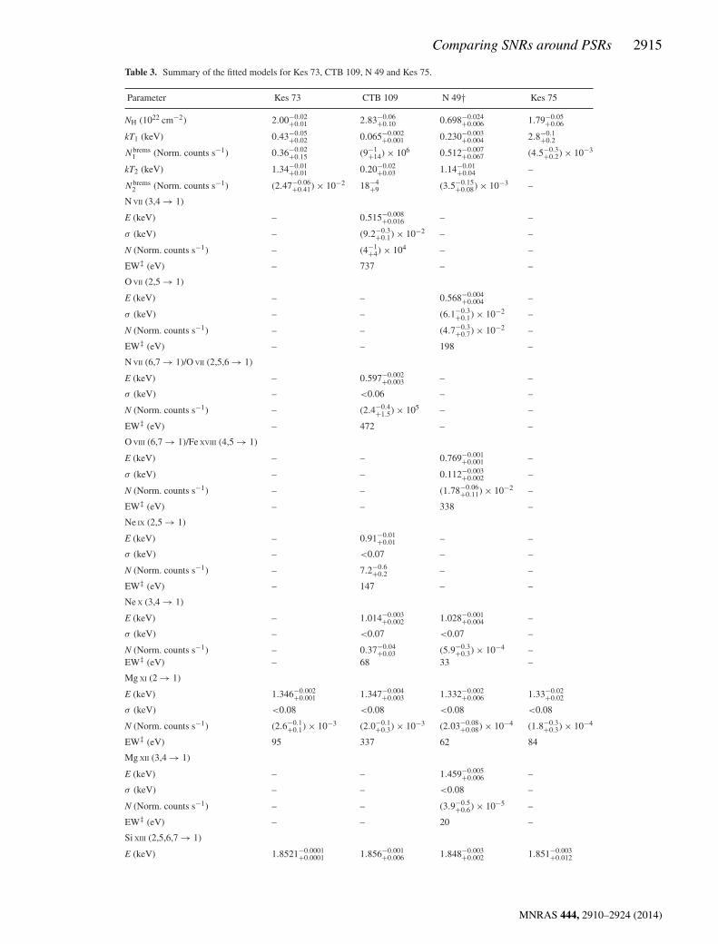
Table 3. Summary of the fitted models for Kes 73, CTB 109, N 49 and Kes 75.

Parameter Kes 73 CTB 109 N 49† Kes 75

NH (1022 cm−2) 2.00−0.02+0.01 2.83−0.06

+0.10 0.698−0.024+0.006 1.79−0.05

+0.06

kT1 (keV) 0.43−0.05+0.02 0.065−0.002

+0.001 0.230−0.003+0.004 2.8−0.1

+0.2

Nbrems1 (Norm. counts s−1) 0.36−0.02

+0.15 (9−1+14) × 106 0.512−0.007

+0.067 (4.5−0.3+0.2) × 10−3

kT2 (keV) 1.34−0.01+0.01 0.20−0.02

+0.03 1.14−0.01+0.04 –

Nbrems2 (Norm. counts s−1) (2.47−0.06

+0.41) × 10−2 18−4+9 (3.5−0.15

+0.08) × 10−3 –

N VII (3,4 → 1)

E (keV) – 0.515−0.008+0.016 – –

σ (keV) – (9.2−0.3+0.1) × 10−2 – –

N (Norm. counts s−1) – (4−1+4) × 104 – –

EW‡ (eV) – 737 – –

O VII (2,5 → 1)

E (keV) – – 0.568−0.004+0.004 –

σ (keV) – – (6.1−0.3+0.1) × 10−2 –

N (Norm. counts s−1) – – (4.7−0.3+0.7) × 10−2 –

EW‡ (eV) – – 198 –

N VII (6,7 → 1)/O VII (2,5,6 → 1)

E (keV) – 0.597−0.002+0.003 – –

σ (keV) – <0.06 – –

N (Norm. counts s−1) – (2.4−0.4+1.5) × 105 – –

EW‡ (eV) – 472 – –

O VIII (6,7 → 1)/Fe XVIII (4,5 → 1)

E (keV) – – 0.769−0.001+0.001 –

σ (keV) – – 0.112−0.003+0.002 –

N (Norm. counts s−1) – – (1.78−0.06+0.11) × 10−2 –

EW‡ (eV) – – 338 –

Ne IX (2,5 → 1)

E (keV) – 0.91−0.01+0.01 – –

σ (keV) – <0.07 – –

N (Norm. counts s−1) – 7.2−0.6+0.2 – –

EW‡ (eV) – 147 – –

Ne X (3,4 → 1)

E (keV) – 1.014−0.003+0.002 1.028−0.001

+0.004 –

σ (keV) – <0.07 <0.07 –

N (Norm. counts s−1) – 0.37−0.04+0.03 (5.9−0.3

+0.3) × 10−4 –EW‡ (eV) – 68 33 –

Mg XI (2 → 1)

E (keV) 1.346−0.002+0.001 1.347−0.004

+0.003 1.332−0.002+0.006 1.33−0.02

+0.02

σ (keV) <0.08 <0.08 <0.08 <0.08

N (Norm. counts s−1) (2.6−0.1+0.1) × 10−3 (2.0−0.1

+0.3) × 10−3 (2.03−0.08+0.08) × 10−4 (1.8−0.3

+0.3) × 10−4

EW‡ (eV) 95 337 62 84

Mg XII (3,4 → 1)

E (keV) – – 1.459−0.005+0.006 –

σ (keV) – – <0.08 –

N (Norm. counts s−1) – – (3.9−0.5+0.6) × 10−5 –

EW‡ (eV) – – 20 –

Si XIII (2,5,6,7 → 1)

E (keV) 1.8521−0.0001+0.0001 1.856−0.001

+0.006 1.848−0.003+0.002 1.851−0.003

+0.012

MNRAS 444, 2910–2924 (2014)

2916 J. Martin et al.

Table 3 – continued

Parameter Kes 73 CTB 109 N 49† Kes 75

σ (keV) <0.02 <0.02 (2.3−0.6+0.6) × 10−2 <0.02

N (Norm. counts s−1) (2.76−0.06+0.06) × 10−3 (7.0−0.2

+0.3) × 10−4 (1.68−0.04+0.06) × 10−4 (2.6−0.1

+0.2) × 10−4

EW‡ (eV) 368 278 299 232

Si XIV (3,4 → 1)

E (keV) – – 1.998−0.002+0.007 –

σ (keV) – – <0.09 –

N (Norm. counts s−1) – – (5.2−0.4+0.3) × 10−5 –

EW‡ (eV) – – 132 –

Si XIII (13 → 1)

E (keV) 2.201−0.010+0.009 – – 2.21−0.02

+0.04

σ (keV) <0.09 – – <0.09

N (Norm. counts s−1) (1.6−0.2+0.2) × 10−4 – – (3.4−0.9

+1.1) × 10−5

EW‡ (eV) 46 – – 45

S XV (2,5,6,7 → 1)

E (keV) 2.452−0.002+0.002 – 2.444−0.005

+0.005 2.437−0.005+0.007

σ (keV) <0.09 – <0.09 <0.09

N (Norm. counts s−1) (8.0−0.3+0.2) × 10−4 – (6.8−0.4

+0.4) × 10−5 (1.09−0.12+0.08) × 10−4

EW‡ (eV) 375 – 299 178

S XV (13 → 1)

E (keV) – – – –

σ (keV) – – – –

N (Norm. counts s−1) – – – –

EW‡ (eV) – – – –

Ar XVII (2,5,6,7 → 1)

E (keV) 3.13−0.01+0.01 – 3.12−0.02

+0.02 –

σ (keV) <0.1 – <0.1 –

N (Norm. counts s−1) (9−1+1) × 10−5 – (7−1

+1) × 10−6 –

EW‡ (eV) 120 – 110 –

Fe XXV (7 → 1)

E (keV) 6.7−0.2+0.2 – – –

σ (keV) 0.5−0.1+0.2 – – –

N (Norm. counts s−1) (2.9−0.6+0.6) × 10−5 – – –

EW‡ (eV) 1890 – – –

χ2r 1.57 (985) 2.05 (477) 1.84 (578) 1.12 (258)

†The absorption column density of N 49 is fitted using the LMC abundances: He = 0.89, C = 0.30, N = 0.12, O= 0.26, Ne = 0.33, Na = 0.30, Mg = 0.32, Al = 0.30, Si = 0.30, S = 0.31, Cl = 0.31, Ar = 0.54, Ca = 0.34, Cr= 0.61, Fe = 0.36, Co = 0.30 and Ni = 0.62. We have added also the galactic absorption NH = 6 × 1020 cm−2.‡ Equivalent width.

The absorption of N 49 has two components: one is related withthe Galactic absorption and the other is the absorption producedby LMC. The Milky Way photoelectric absorption towards N 49is fixed as NH = 6 × 1020 cm−2 (Dickey & Lockman 1990; Parket al. 2012). We include a second absorption component to take intoaccount the absorption column density for LMC, where we use theabundances given by Russell & Dopita (1992), Hughes, Hayashi& Koyama (1998) and Park et al. (2012). We obtain an absorptioncolumn density of NH = 0.7 × 1022 cm−2 for the LMC contribution.The continuum is represented by two Bremsstrahlung models withtemperatures of 0.23 and 1.14 keV. In this case, we have detectednine lines: O VII at 0.57 keV (EW = 0.20 keV), O VIII/Fe XVIII at

0.77 keV (EW = 0.34 keV), Ne X at 1.03 keV (EW = 33 eV), Mg XI

at 1.33 keV (EW = 62 eV), Mg XII at 1.46 keV (EW = 20 eV), Si XIII

at 1.85 keV (EW = 0.30 keV), Si XIV at 2.00 keV (EW = 0.13 keV),S XV at 2.44 keV (EW = 0.30 keV) and Ar XVII at 3.12 keV(EW = 0.11 keV).

3.4 Kes 75

Kes 75 (G29.7−0.3) is a composite SNR. The X-ray emis-sion of the partial shell is extended in two clouds in thesouth-west and south-east part of the image (see Fig. 1). Itwas observed first in X-rays by Einstein (Becker, Helfand &

MNRAS 444, 2910–2924 (2014)

Comparing SNRs around PSRs 2917

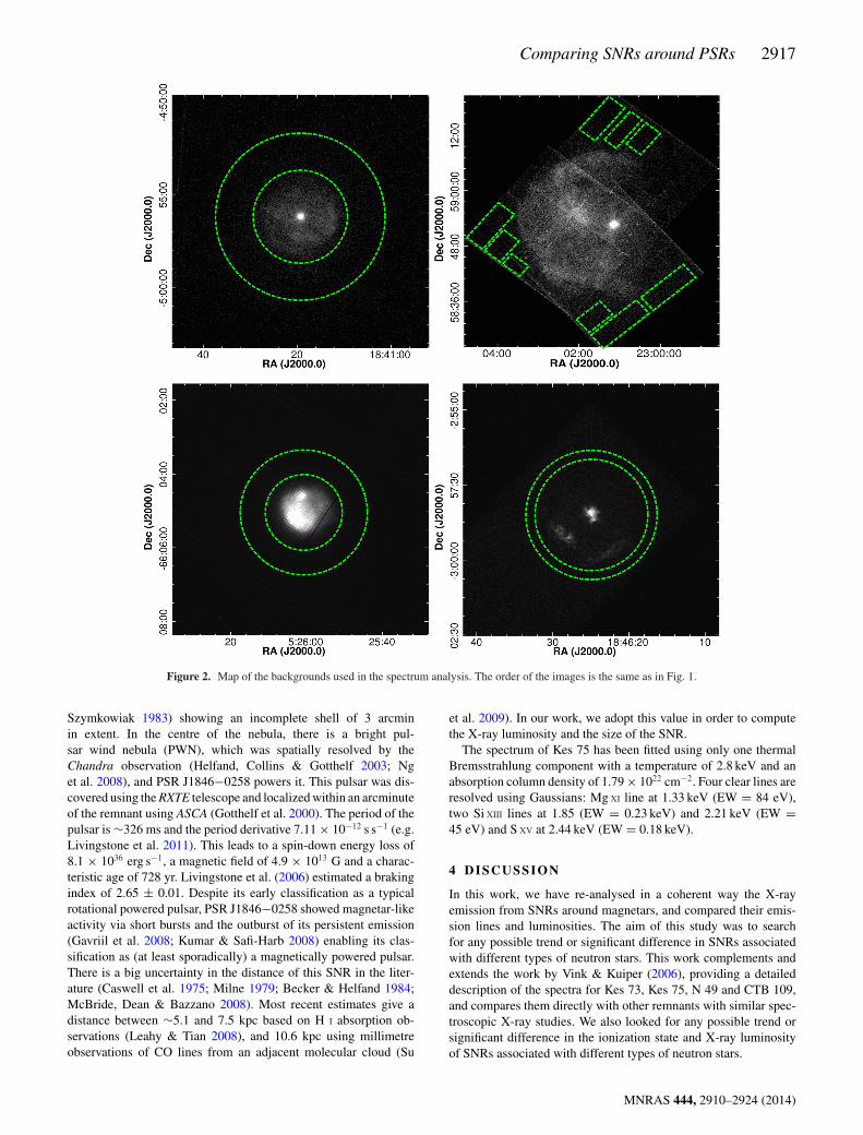
Figure 2. Map of the backgrounds used in the spectrum analysis. The order of the images is the same as in Fig. 1.

Szymkowiak 1983) showing an incomplete shell of 3 arcminin extent. In the centre of the nebula, there is a bright pul-sar wind nebula (PWN), which was spatially resolved by theChandra observation (Helfand, Collins & Gotthelf 2003; Nget al. 2008), and PSR J1846−0258 powers it. This pulsar was dis-covered using the RXTE telescope and localized within an arcminuteof the remnant using ASCA (Gotthelf et al. 2000). The period of thepulsar is ∼326 ms and the period derivative 7.11 × 10−12 s s−1 (e.g.Livingstone et al. 2011). This leads to a spin-down energy loss of8.1 × 1036 erg s−1, a magnetic field of 4.9 × 1013 G and a charac-teristic age of 728 yr. Livingstone et al. (2006) estimated a brakingindex of 2.65 ± 0.01. Despite its early classification as a typicalrotational powered pulsar, PSR J1846−0258 showed magnetar-likeactivity via short bursts and the outburst of its persistent emission(Gavriil et al. 2008; Kumar & Safi-Harb 2008) enabling its clas-sification as (at least sporadically) a magnetically powered pulsar.There is a big uncertainty in the distance of this SNR in the liter-ature (Caswell et al. 1975; Milne 1979; Becker & Helfand 1984;McBride, Dean & Bazzano 2008). Most recent estimates give adistance between ∼5.1 and 7.5 kpc based on H I absorption ob-servations (Leahy & Tian 2008), and 10.6 kpc using millimetreobservations of CO lines from an adjacent molecular cloud (Su

et al. 2009). In our work, we adopt this value in order to computethe X-ray luminosity and the size of the SNR.

The spectrum of Kes 75 has been fitted using only one thermalBremsstrahlung component with a temperature of 2.8 keV and anabsorption column density of 1.79 × 1022 cm−2. Four clear lines areresolved using Gaussians: Mg XI line at 1.33 keV (EW = 84 eV),two Si XIII lines at 1.85 (EW = 0.23 keV) and 2.21 keV (EW =45 eV) and S XV at 2.44 keV (EW = 0.18 keV).

4 D I SCUSSI ON

In this work, we have re-analysed in a coherent way the X-rayemission from SNRs around magnetars, and compared their emis-sion lines and luminosities. The aim of this study was to searchfor any possible trend or significant difference in SNRs associatedwith different types of neutron stars. This work complements andextends the work by Vink & Kuiper (2006), providing a detaileddescription of the spectra for Kes 73, Kes 75, N 49 and CTB 109,and compares them directly with other remnants with similar spec-troscopic X-ray studies. We also looked for any possible trend orsignificant difference in the ionization state and X-ray luminosityof SNRs associated with different types of neutron stars.

MNRAS 444, 2910–2924 (2014)

2918 J. Martin et al.

Figure 3. Spectra obtained for the Kes 73, CTB 109, N 49 and Kes 75. We used the EPIC PN (in black), MOS 1 (in red) and MOS 2 (in green) datasimultaneously to fit the models.

4.1 Spectral lines comparison with other SNRs

X-ray spectra of SNRs are usually fit with plasma models (seealso Table 2). In this work, we proceed to fit the spectra of Kes73, CTB 109, N 49 and Kes 75 using a thermal Bremsstrahlungmodel for the continuum emission and Gaussians for the lines. Ourmain aim is to have an estimate of line centroid energy, to identifyit properly. We have then used the simplest continuum model to

reduce the free parameters of the fit.2 One could expect that theexcess of rotational energy released by the magnetar during thealpha-dynamo process could be stored in the ionization level of

2 Note that in the 0.5–1 keV the detection of spectral lines are dependent onabsorption model we adopted.

MNRAS 444, 2910–2924 (2014)

Comparing SNRs around PSRs 2919

Table 4. Summary of line detections in X-ray for some important SNRs compared with lines detected in our analysis. The references are [1]Bleeker et al.(2001), [2]Borkowski et al. (2010), [3]Cassam-Chenaı et al. (2004), [4]Decourchelle et al. (2001), [5]Hayato et al. (2010), [6]Hwang & Gotthelf (1997),[7]Hwang, Petre & Flanagan (2008), [8]Kinugasa & Tsunemi (1987), [9]Maeda et al. (2009), [10]Miceli et al. (2009), [11]Park et al. (2007), [12]Reynoldset al. (2007), [13]Tamagawa et al. (2009), [14]Vink et al. (2004), [15]Warren & Hughes (2004), [16]Willingale et al. (2002), [17]Winkler et al. (1981a),[18]Winkler et al. (1981b), [19]Yamaguchi et al. (2008).

SNR Galaxy Age (yr) ElementO VII O VIII O VIII Ne IX Ne X Ne X

(2,5,7 → 1) (3,4 → 1) (6,7 → 1) (2,5 → 1) (3,4 → 1) (6,7 → 1)(0.574 KeV) (0.653 KeV) (0.774 KeV) (0.915 KeV) (1.022 KeV) (1.21 KeV)

Kes 73 MW 1100–1500CTB 109 MW 7900–9700 X XKes 75 MW 900–4300N 49 LMC 5000 X X X XG1.9+1.3 [2] MW 110–170Kepler [3],[8],[12] MW 408 XTycho [4],[5],[6],[13] MW 440 XSN1006 [10],[19] MW 1006 X X XCas A [1],[9],[16] MW 316–352 X X X X XMSH11-54 [11],[14] MW 2930–3050 X X X X XPuppis A [7],[17],[18] MW 3700–5500 X X X X X XB0509-67.5 [15] LMC 400 X X X

Mg XI Mg XII Si XIII Si XIV Si XIII S XV

(2,5,6,7 → 1) (3,4 → 1) (2,5,6,7 → 1) (3,4 → 1) (13 → 1) (2,5,6,7 → 1)(1.35 KeV) (1.47 KeV) (1.86 KeV) (2.00 KeV) (2.18 KeV) (2.46 KeV)

Kes 73 MW 1100–1500 X X X XCTB 109 MW 7900–9700 X XKes 75 MW 900–4300 X X X XN 49 LMC 5000 X X X X XG1.9+1.3 MW 110–170 X X XKepler MW 408 X X X X XTycho MW 440 X X X XSN1006 MW 1006 X XCas A MW 316–352 X X X X X XMSH11−54 MW 2930–3050 X X X XPuppis A MW 3700–5500 X X X XB0509−67.5 LMC 400 X X X X

S XV Ar XVII Ca XIX Fe XXV

(13 → 1) (2,5,6,7 → 1) (2,5,6,7 → 1) K-shell(2.88 KeV) (3.13 KeV) (3.89 KeV) (6.65 KeV)

Kes 73 MW 1100–1500 X XCTB 109 MW 7900–9700Kes 75 MW 900–4300N 49 LMC 5000 XG1.9+1.3 MW 110–170 X X XKepler MW 408 X X X XTycho MW 440 X X X XSN1006 MW 1006Cas A MW 316–352 X X X XMSH11−54 MW 2930–3050Puppis A MW 3700–5500B0509−67.5 LMC 400 X X X

the lines present in the spectrum. If the energy release is higherthan in a normal SNR, heavy elements such as silicon (Si), sulphur(S), argon (Ar), calcium (Ca) or iron (Fe) could be systematicallyat a higher state of ionization. In Table 4, we collected all SNRswith detailed spectroscopic studies in the literature and we see thatthe typical elements detected are O VII, O VIII, Ne IX, Ne X, Mg XI,Mg XII, Si XIII, Si XIV, S XV, S XVI, Ar XVII, Ca XIX and Fe XXV. Theonly lines detected in all four of the spectra are the Mg XI line at1.33 keV and Si XIII at 1.85 keV. For comparison, we also fitted thespectra of the SNRs using a vnei model (e. g. Borkowski, Lyerly& Reynolds 2001). The results are summarized in the Table 2. We

have added a thermal Bremsstrahlung component in some cases.The temperature of the vnei plasma is always higher than for thethermal Bremsstrahlung, with the exception of N 49 in which thetemperature for vnei is 0.17 keV (0.99 keV for Bremsstrahlung).The abundances obtained in both models show similar tendencies.For Kes 73 and N 49, the abundances of Si and S are quite abovethe solar ones. CTB 109 shows low abundances with respect tothe solar ones for O, Ne, Mg, Si and Fe. Due to the complexityof the N 49 spectrum, some lines have not been reproduced well bythe plasma models and we have added them using Gaussian profilesto improve the fit. In summary, our spectroscopic X-ray analysis

MNRAS 444, 2910–2924 (2014)

2920 J. Martin et al.

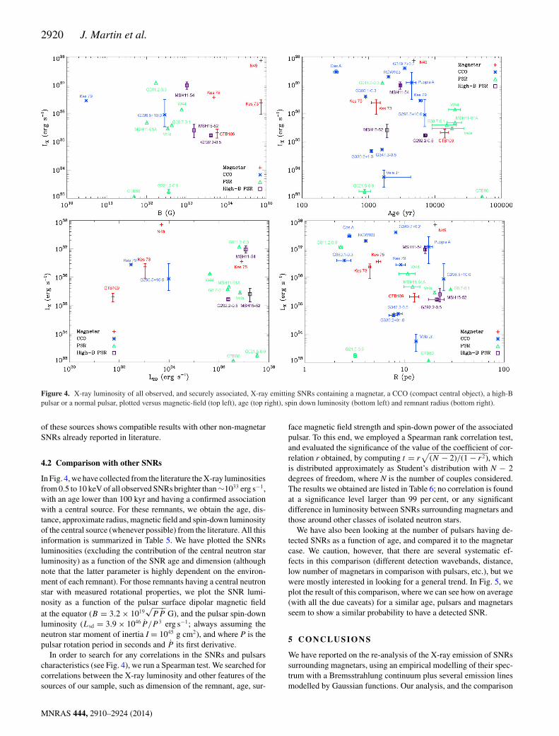
Figure 4. X-ray luminosity of all observed, and securely associated, X-ray emitting SNRs containing a magnetar, a CCO (compact central object), a high-Bpulsar or a normal pulsar, plotted versus magnetic-field (top left), age (top right), spin down luminosity (bottom left) and remnant radius (bottom right).

of these sources shows compatible results with other non-magnetarSNRs already reported in literature.

4.2 Comparison with other SNRs

In Fig. 4, we have collected from the literature the X-ray luminositiesfrom 0.5 to 10 keV of all observed SNRs brighter than ∼1033 erg s−1,with an age lower than 100 kyr and having a confirmed associationwith a central source. For these remnants, we obtain the age, dis-tance, approximate radius, magnetic field and spin-down luminosityof the central source (whenever possible) from the literature. All thisinformation is summarized in Table 5. We have plotted the SNRsluminosities (excluding the contribution of the central neutron starluminosity) as a function of the SNR age and dimension (althoughnote that the latter parameter is highly dependent on the environ-ment of each remnant). For those remnants having a central neutronstar with measured rotational properties, we plot the SNR lumi-nosity as a function of the pulsar surface dipolar magnetic fieldat the equator (B = 3.2 × 1019

√P P G), and the pulsar spin-down

luminosity (Lsd = 3.9 × 1046P /P 3 erg s−1; always assuming theneutron star moment of inertia I = 1045 g cm2), and where P is thepulsar rotation period in seconds and P its first derivative.

In order to search for any correlations in the SNRs and pulsarscharacteristics (see Fig. 4), we run a Spearman test. We searched forcorrelations between the X-ray luminosity and other features of thesources of our sample, such as dimension of the remnant, age, sur-

face magnetic field strength and spin-down power of the associatedpulsar. To this end, we employed a Spearman rank correlation test,and evaluated the significance of the value of the coefficient of cor-relation r obtained, by computing t = r

√(N − 2)/(1 − r2), which

is distributed approximately as Student’s distribution with N − 2degrees of freedom, where N is the number of couples considered.The results we obtained are listed in Table 6; no correlation is foundat a significance level larger than 99 per cent, or any significantdifference in luminosity between SNRs surrounding magnetars andthose around other classes of isolated neutron stars.

We have also been looking at the number of pulsars having de-tected SNRs as a function of age, and compared it to the magnetarcase. We caution, however, that there are several systematic ef-fects in this comparison (different detection wavebands, distance,low number of magnetars in comparison with pulsars, etc.), but wewere mostly interested in looking for a general trend. In Fig. 5, weplot the result of this comparison, where we can see how on average(with all the due caveats) for a similar age, pulsars and magnetarsseem to show a similar probability to have a detected SNR.

5 C O N C L U S I O N S

We have reported on the re-analysis of the X-ray emission of SNRssurrounding magnetars, using an empirical modelling of their spec-trum with a Bremsstrahlung continuum plus several emission linesmodelled by Gaussian functions. Our analysis, and the comparison

MNRAS 444, 2910–2924 (2014)

Comparing SNRs around PSRs 2921

Table 5. SNRs considered in our X-ray luminosity analysis. The data without references is extracted from this work or deduced from the data obtainedin the literature. The references are [1]Aharonian et al. (2007), [2]Archibald et al. (2013), [3]Aschenbach, Egger & Trumper (1995), [4]Becker et al. (2012),[5]Bietenholz & Bartel (2008), [6]Blanton & Helfand (1996), [7]Carter, Dickel & Bomans (1997), [8]Case & Bhattacharya (1998), [9]Caswell et al. (2004),[10]Chandra SNR catalogue∗, [11]Cox et al. (1999), [12]Dodson, McCulloch & Lewis (2002), [13]Dodson et al. (2003), [14]Dubner et al. (2013), [15]Fang &Zhang (2010), [16]Ferrand & Safi-Harb (2012), [17]Fesen et al. (2006), [18]Fesen et al. (2012), [19]Finley & Oegelman (1994), [20]Frail et al. (1996), [21]Gaensleret al. (1999), [22]Gaensler & Wallace (2003), [23]Gaensler et al. (2008), [24]Giacani et al. (2000), [25]Gotthelf, Petre & Vasisht (1999a), [26]Gotthelf et al.(2000), [27]Halpern & Gotthelf (2010), [28]Hobbs et al. (2004), [29]Hughes et al. (2003), [30]Kaspi et al. (2001), [31]Katsuda, Tsunemi & Mori (2008), [32]Kellettet al. (1987), [33]Kothes et al. (2002), [34]Koyama et al. (1997), [35]Kuiper et al. (2006), [36]Kulkarni et al. (2003), [37]Kumar, Safi-Harb & Gonzalez (2012),[38]Lazendic et al. (2003), [39]Lazendic et al. (2005), [40]Livingstone et al. (2011), [41]Livingstone & Kaspi (2011), [42]Lu & Aschenbach (2000), [43]Matheson& Safi-Harb (2010), [44]Matsui, Long & Tuohy (1988), [45]Mereghetti, Tiengo & Israel (2002), [46]Mineo et al. (2001), [47]Park et al. (2009), [48]Park et al.(2012), [49]Pavlov et al. (2001), [50]Pavlov et al. (2002), [51]Pfeffermann & Aschenbach (1996), [52]Ray et al. (2011), [53]Reed et al. (1995), [54]Reynoso et al.(1995), [55]Reynoso et al. (2004), [56]Rho et al. (1994), [57]Roger et al. (1988), [58]Roy, Gupta & Lewandowski (2012), [59]Safi-Harb & Oegelman (1994),[60]Safi-Harb, Oegelman & Finley (1995), [61]Sanbonmatsu & Helfand (1992), [62]Sasaki et al. (2013), [63]Seward et al. (2003), [64]Slane et al. (2002), [65]Strom& Stappers (2000), [66]Su et al. (2009), [67]Sun et al. (2004), [68]Tam & Roberts (2003), [69]Tian & Leahy (2008a), [70]Torii et al. (1999), [71]Torii et al. (2006),[72]Vasisht & Gotthelf (1997), [73]Vink & Kuiper (2006), [74]Wang et al. (2000), [75]Weltevrede, Johnston & Espinoza (2011), [76]Winkler et al. (2009), [77]Yuanet al. (2010), [78]Zeiger et al. (2008).

SNRs with magnetars

Name Central source Distance Radius Age E Bs FX LX

(kpc) (pc) (kyr) (erg s−1) (G) (erg cm−2 s−1) (erg s−1)

Kes 75 J1846−0258 [26] 10.6 [66] 5.5−0.3+0.3 [10] 0.9 [6] 8.06 × 1036 [40] 4.88 × 1013 [40] 2.69 × 10−10 3.61 × 1036

Kes 73 1E 1841−045 [72] 6.7−1.0+1.8 [61] 4.5−0.1

+0.1 [10] 1.3−0.2+0.2 [73] 1.08 × 1033 [35] 7.34 × 1014 [35] 4.39 × 10−10 (2.36−0.65

+1.43) × 1036

N 49 RX J0526−6604 [36] 50 [36] 20.4 [10] 4.8 [48] 4.92 × 1033 [36] 7.32 × 1014 [36] 2.41 × 10−10 7.21 × 1037

CTB 109 1E 2259+586 [2] 3−0.5+0.5 [33] 12.6−1.3

+1.3 [10] 14−2+2 [62] 5.54 × 1031 [2] 5.84 × 1013 [2] 1.94 × 10−10 (2.09−0.64

+0.75) × 1035

SNRs with CCOs

Cas A CXO J2323+5848 [45] 3.4−0.1+0.3 [53] 2.8−0.1

+0.1 [10] 0.326−27+27 [17] – – 2.06 × 10−8 [10] (2.85−0.20

+0.50) × 1037 [10]

G350.1−0.3 XMMU J1720−3726 [23] 4.5 [23] 2.5−0.4+0.4 [10] 0.9 [23] – – 1.64 × 10−9 [10] 3.97 × 1036 [10]

G330.2+1.0 CXOU J1601−5133 [47] 4.9−0.3+0.3 [53] 7.8−0.8

+0.8 [10] 1.1 [47] – – 1.60 × 10−11 [71] (4.60−0.55+0.57) × 1034 [71]

G347.3−0.5 1 WGA J1713−3949 [38] 1 [34] 8.7−0.8+0.8 [18] 1.6 [18] – – 4.40 × 10−10 [51] 5.26 × 1034

Vela Jr. CXOU J0852−4617 [49] 0.75−0.55+0.25 [35] 13.1 [10] 1.7−0

+2.6 [35] – – 8.30 × 10−11 [1] (5.58−3.10+4.34) × 1033

RCW 103 1E 1613−5055 [25] 3.1 [55] 4.1−0.1+0.1 [10] 2 [7] – – 1.70 × 10−8 [10] 1.95 × 1037

G349.7+0.2 CXOU J1718−3726 [39] 22.4 [20] 8.2 [39] 3.5 [39] – – 6.50 × 10−10 [39] 3.90 × 1037

Puppis A RX J0822−4300 [4] 2.2−0.3+0.3 [54] 17.5−1.7

+1.7 [16] 4.45−0.75+0.75 [4] – – 2.16 × 10−8 (1.20−0.90

+1.55) × 1037 [14]

Kes 79 J1852+0040 [63] 7.1 [8] 9.2−1.0+1.0 [10] 6.0−0.2

+0.4 [67] 2.96 × 1032 [27] 3.05 × 1010 [27] 4.64 × 10−10 [67] 2.80 × 1036 [67]

G296.5+10.0 1E 1207−5209 [24] 2.1−0.8+1.8 [24] 24.8 [32] 7 [57] 9.58 × 1033 [50] 2.83 × 1012 [50] 1.67 × 10−9 [44] (8.81−5.40

+21.60) × 1034

SNRs with high-B PSRs

MSH 15−52 J1513−5908 [21] 5.2−1.4+1.4 [15] 22.7 [46] 1.9 [15] 1.75 × 1037 [41] 1.54 × 1013 [41] 7.80 × 10−11 [46] (2.52−1.17

+1.54) × 1035

MSH 11−54 J1124−5916 [29] 6.2−0.9+0.9 [22] 16.2−0.2

+0.2 [10] 2.99−0.06+0.06 [76] 1.19 × 1037 [52] 1.02 × 1013 [52] 2.09 × 10−9 [10] (9.61−2.59

+2.99) × 1036

G292.2−0.5 J1119−6127 [37] 8.4−0.4+0.4 [9] 21.1−3.8

+3.8 [10] 7.1−0.2+0.5 [37] 2.34 × 1036 [75] 4.10 × 1013 [75] 1.98 × 10−11 [37] (1.67−0.15

+0.16) × 1035

SNRs with normal PSRs

G21.5−0.9 J1833−1034 [43] 4.7−0.4+0.4 [69] 3.2−0.1

+0.1 [10] 0.87−1.5+2.0 [5] 3.37 × 1037 [58] 3.58 × 1012 [58] 6.69 × 10−13 (1.77−0.31

+0.29) × 1033 [43]

G11.2−0.3 J1811−1925 [70] 5 [30] 2.3−0.1+0.1 [10] 1.616 [68] 6.42 × 1036 [70] 1.71 × 1012 [70] 3.98 × 10−9 [10] 1.19 × 1037 [10]

G8.7−0.1 J1803−2137 [19] 4 [19] 29.1 [19] 15−6+6 [19] 2.22 × 1036 [77] 4.92 × 1012 [77] 2.00 × 10−10 [19] 3.83 × 1035

Vela J0835−4510 [3] 0.287−0.017+0.019 [13] 20.1 [42] 18−9

+9 [3] 6.92 × 1036 [12] 3.38 × 1012 [12] 2.94 × 10−8 (2.90−0.34+0.39) × 1035 [42]

MSH 11−61A J1105−6107 [64] 7 [64] 12.1−2.2+2.2 [64] 20−5

+5 [64] 2.48 × 1036 [74] 1.01 × 1012 [74] 8.06 × 10−11 [10] 4.71 × 1035 [10]

W 44 J1856+0113 [11] 2.5 [11] 10.8−2.0+2.0 [11] 20−4

+4 [11] 4.30 × 1035 [28] 7.55 × 1012 [28] 1.80 × 10−9 [56] 1.35 × 1036

CTB 80 J1952+3252 [60] 2 [65] 1.5 [60] 51 [78] 3.74 × 1036 [28] 4.86 × 1011 [28] 2.40 × 10−12 1.15 × 1033 [59]

∗http://hea-www.cfa.harvard.edu/ChandraSNR/

of the emission of those remnants with other bright SNR surround-ing normal pulsars suggest the following conclusions.

(i) We find no evidence of generally enhanced ionization states inthe elements observed in magnetars’ SNRs compared to remnantsobserved around lower magnetic pulsars.

(ii) No significant correlation is observed between the SNRs’X-ray luminosities and the pulsar magnetic fields.

(iii) We show evidence that the percentage of magnetars andpulsars hosted in a detectable SNR are very similar, at a similar age.

Our findings do not support the claim of magnetars being formedvia more energetic SNe, or having a large rotational energy budgetat birth that is released in the surrounding medium in the first phasesof the magnetar formation. However, we note that although we donot find any hint in the SNRs to support such an idea, we cannotexclude that: (1) most of the rotational energy has been emittedvia neutrinos or gravitational waves, hence with no interaction withthe remnant; or (2) we are restricted to a very small sample, andwith larger statistics some correlation might be observed in thefuture.

MNRAS 444, 2910–2924 (2014)

2922 J. Martin et al.

Table 6. Spearman correlation coefficient (r), number ofcouples considered (N) and probability that the two samplesare not correlated (p) evaluated by comparing the X-ray lu-minosity of the sources of our sample with the age, radius,surface magnetic field strength and spin-down luminosity.

Parameters r N p

LX versus age − 0.158 24 0.46LX versus radius − 0.245 24 0.25LX versus B 0.271 16 0.31LX versus Lsd − 0.309 16 0.25

Figure 5. Percentage of pulsars and magnetars having a detected SNR as afunction of the age.

AC K N OW L E D G E M E N T S

This work was supported by grants AYA2012-39303, SGR2009-811, iLINK 2011-0303 and the NewCOMPSTAR MP1304 COSTAction. NR is supported by a Ramon y Cajal fellowship and byan NWO Vidi Award. AP is supported by a Juan de la Ciervafellowship. We are indebted to Samar Safi-Harb and Harsha Kumarfor providing the Chandra data on Kes 75, and for useful comments.We also thank Manami Sasaki and the referee for comments andsuggestions that improved the manuscript.

R E F E R E N C E S

Aharonian F. et al., 2007, ApJ, 661, 236Archibald R. F. et al., 2013, Nature, 497, 591Arnaud K. A., 1996, Jacoby G., Barnes J., eds, ASP Conf. Ser. Vol. 101,

Astronomical Data Analysis Software and Systems V. Astron. Soc. Pac.,San Francisco, p. 17

Aschenbach B., Egger R., Trumper J., 1995, Nature, 373, 587Banas K. R., Hughes J. P., Bronfman L., Nyman L., 1997, ApJ, 480, 607Becker R. H., Helfand D. J., 1984, ApJ, 283, 154Becker R. H., Helfand D. J., Szymkowiak A. E., 1983, ApJ, 268, L93Becker W., Prinz T., Winkler P. F., Petre R., 2012, ApJ, 755, 141Bietenholz M. F., Bartel N., 2008, MNRAS, 386, 1411Blanton E. L., Helfand D. J., 1996, ApJ, 470, 961Bleeker J. A., Willingale R., van der Heyden K., Dennerl K., Kaastra J. S.,

Aschenbach B., Vink J., 2001, A&A, 365, L225Borkowski K. J., Lyerly W. J., Reynolds S. P., 2001, ApJ, 548, 820Borkowski K. J., Reynolds S. P., Green D. A., Hwang U., Petre R., Krish-

namurthy K., Willett R., 2010, ApJ, 724, L161

Bucciantini N., Metzger B. D., Thompson T. A., Quataert E., 2012, MNRAS,419, 1537

Carter L. M., Dickel J. R., Bomans D. J., 1997, PASP, 109, 990Case G. L., Bhattacharya D., 1998, ApJ, 504, 761Cassam-Chenaı G., Decourchelle A., Ballet J., Hwang U., Hughes J. P.,

Petre R., 2004, A&A, 414, 545Caswell J. L., Murray J. D., Roger R. S., Cole D. J., Cooke D. J., 1975,

A&A, 45, 239Caswell J. L., McClure-Griffiths N. M., Cheung M. C. M., 2004, MNRAS,

352, 1405Clark J. S., Ritchie B. W., Najarro F., Langer N., Negueruela I., 2014, A&A,

565, 90Cox D. P., Shelton R. L., Maciejewski W., Smith R. K., Plewa T., Pawl A.,

Rozyczka M., 1999, ApJ, 524, 179Davies B., Figer D. F., Kudritzki R.-P., Trombley C., Kouveliotou C.,

Wachter S., 2009, ApJ, 707, 844Decourchelle A. et al., 2001, A&A, 365, L218Dickey J. M., Lockman F. J., 1990, ARA&A, 28, 215Dodson R. G., McCulloch P. M., Lewis D. R., 2002, ApJ, 564, L85Dodson R. G., Legge D., Reynolds J. E., McCulloch P. M., 2003, ApJ, 596,

1137Donati J. F., Babel J., Harries T. J., Howarth I. D., Petit P., Semel M., 2002,

MNRAS, 333, 55Donati J. F., Howarth I. D., Bouret J. C., Petit P., Catala C., Landstreet J.,

2006, MNRAS, 365, 6Dubner G., Loiseau N., Rodrıguez-Pascual P., Smith M. J. S., Giacani E.,

Castelletti G., 2013, A&A, 555, A9Duncan R. C., Thompson C., 1992, ApJ, 392, L9Duncan R. C., Thompson C., 1996, in Rothschild R. E., Lingenfelter R.

E., eds, AIP Conf. Proc. Vol. 366, High Velocity Neutron Stars andGamma-Ray Bursts. Am. Inst. Phys., New York, p. 111

Fahlman G. G., Gregory P. C., 1983, in Danziger J., Gorenstein P., eds,Proc. IAU Symp. 101, Supernova Remnants and Their X-Ray Emission.Kluwer, Dordrecht, p. 445

Fang J., Zhang L., 2010, A&A, 515, 20Ferrand G., Safi-Harb S., 2012, Adv. Space Res., 49, 1313Ferrario L., Wickramasinghe D., 2006, MNRAS, 367, 1323Fesen R. A. et al., 2006, ApJ, 645, 283Fesen R. A., Kremer R., Patnaude D., Milisavljevic D., 2012, AJ, 143, 27Figer D. F., Najarro F., Gaballe T. R., Blum R. D., Kudritzki R. P., 2005,

ApJ, 622, L49Finley J. P., Oegelman H., 1994, ApJ, 434, L25Frail D. A., Goss W. M., Reynoso E. M., Giacani E. B., Green A. J., Otrupcek

R., 1996, AJ, 111, 1651Fuchs Y., Mirabel F., Chaty S., Claret A., Cesarsky C. J., Cesarsky D. A.,

1999, A&A, 350, 891Gaensler B. M., Wallace B. J., 2003, ApJ, 594, 326Gaensler B. M., Brazier K. T. S., Manchester R. N., Johnston S., Green A.

J., 1999, MNRAS, 305, 724Gaensler B. M., Slane P. O., Gotthelf E. V., Vasisht G., 2001, ApJ, 486,

L133Gaensler B. M., McClure-Griffiths N. M., Oey M. S., Haverkorn M., Dickey

J. M., Green A. J., 2005, ApJ, 620, L95Gaensler B. M. et al., 2008, ApJ, 680, L37Gavriil F. P., Gonzalez M. E., Gotthelf E. V., Kaspi V. M., Livingstone M.

A., Woods P. M., 2008, Science, 319, 1802Giacani E. B., Dubner G. M., Green A. J., Goss W. M., Gaensler B. M.,

2000, AJ, 119, 281Gotthelf E. V., Vasisht G., 1997, ApJ, 486, L133Gotthelf E. V., Petre R., Vasisht G., 1999, ApJ, 514, L107Gotthelf E. V., Vasisht G., Dotani T., 1999, ApJ, 522, L49Gotthelf E., Vasisht G., Boylan-Kolchin M., Torii K., 2000, ApJ, 542, L37Gregory P. C., Fahlman G. G., 1980, Nature, 287, 805Halpern J. P., Gotthelf E. V., 2010, ApJ, 709, 436Hayato A. et al., 2010, ApJ, 725, 894Heger A., Woosley S. E., Spruit H. C., 2005, ApJ, 626, 350Helfand D. J., Becker R. H., Hawkins G., White R. L., 1994, ApJ, 434, 627Helfand D. J., Collins B. F., Gotthelf E. V., 2003, ApJ, 582, 783

MNRAS 444, 2910–2924 (2014)

Comparing SNRs around PSRs 2923

Hillebrandt W., Niemeyer J. C., 2000, ARA&A, 38, 191Hobbs G., Lyne A. G., Kramer M., Martin C. E., Jordan C., 2004, MNRAS,

353, 1311Hughes J. P., Hayashi I., Koyama K., 1998, ApJ, 505, 732Hughes J. P., Slane P. O., Park S., Roming P. W. A., Burrows D. N., 2003,

ApJ, 591, L139Hurford A. P., Fesen R. A., 1995, MNRAS, 277, 549Hwang U., Gotthelf E. V., 1997, ApJ, 475, 665Hwang U., Petre R., Flanagan K. A., 2008, ApJ, 676, 378Iwasawa K., Koyama K., Halpern J. P., 1992, PASJ, 44, 9Kaspi V. M., Roberts M. E., Vasisht G., Gotthelf E. V., Pivovaroff M., Kawai

N., 2001, ApJ, 560, 371Katsuda S., Tsunemi H., Mori K., 2008, ApJ, 678, L35Kellett B. J., Branduardi-Raymont G., Culhane J. L., Mason I. M., Mason

K. O., Whitehouse D. R., 1987, MNRAS, 225, 199Kinugasa K., Tsunemi H., 1999, PASJ, 51, 239Kothes R., Uyaniker B., Yar A., 2002, ApJ, 576, 169Koyama K., Kinugasa K., Matsuzaki K., Nishiuchi M., Sugizaki M., Torii

Ken’ichi., Yamauchi S., Aschenbach B., 1997, PASJ, 49, L7Kriss G. A., Becker R. H., Helfand D. J., Canizares C. R., 1985, ApJ, 288,

703Kuiper L., Hermsen W., den Hartog P. R., Collmar W., 2006, ApJ, 645, 556Kulkarni S. R., Kaplan D. L., Marshall H. L., Frail D. A., Murakami T.,

Yonetoku D., 2003, ApJ, 585, 948Kumar H. S., Safi-Harb S., 2008, ApJ, 678, 43Kumar H. S., Safi-Harb S., Gonzalez M. E., 2012, ApJ, 754, 96Kumar H. S., Safi-Harb S., Slane P. O., Gotthelf E. V., 2014, ApJ, 781, 41Lazendic J. S., Slane P. O., Gaensler B. M., Plucinsky P. P., Hughes J. P.,

Galloway D. K., Crawford F., 2003, ApJ, 593, L27Lazendic J. S., Slane P. O., Hughes J. P., Chen Y., Dame T. M., 2005, ApJ,

618, 733Leahy D. A., Tian W. W., 2008, A&A, 480, L25Livingstone M. A., Kaspi V. M., 2011, ApJ, 742, 31Livingstone M. A., Kaspi V. M., Gotthelf E. V., Kuiper L., 2006, ApJ, 647,

1286Livingstone M. A., Ng C.-Y., Kaspi V. M., Gavriil F. P., Gotthelf E. V., 2011,

ApJ, 730, 66Lopez L. A., Ramirez-Ruiz E., Huppenkothen D., Badenes C., Pooley D.

A., 2011, ApJ, 732, 114Lu F. J., Aschenbach B., 2000, A&A, 362, 1083McBride V. A., Dean A. J., Bazzano F., 2008, A&A, 477, 249Maeda Y. et al., 2009, PASJ, 61, 1217Matheson H., Safi-Harb S., 2010, ApJ, 724, 572Matsui Y., Long K. S., Tuohy I. R., 1988, ApJ, 329, 838Mazets E. P., Golenetskii S. V., Il’inskii V. N., Aptekar R. L., Guryan Y. A.,

1979, Nature, 282, 587Mereghetti S., 2008, A&AR, 15, 225Mereghetti S., Tiengo A., Israel G. L., 2002, ApJ, 569, 275Metzger B. D., Giannios D., Thompson T. A., Bucciantini N., Quataert E.,

2011, MNRAS, 413, 2031Miceli M. et al., 2009, A&A, 501, 239Milne D. K., 1979, Aust. J. Phys., 32, 83Mineo T., Cusumano G., Maccarone M. C., Massaglia S., Massaro E.,

Trussoni E., 2001, A&A, 380, 695Muno M. P. et al., 2006, ApJ, 636, L41Ng C.-Y., Slane P. O., Gaensler B. M., Hughes J. P., 2008, ApJ, 686, 508Oskinova L. M., Todt H., Ignace R., Brown J. C., Cassinelli J. P., Hamann

W.-R., 2011, MNRAS, 416, 1456Park S., Hughes J. P., Slane P. O., Burrows D. N., Gaensler B. M.,

Ghavamian P., 2007, ApJ, 670, L121Park S., Kargaltsev Oleg., Pavlov G. G., Mori K., Slane P. O., Hughes J. P.,

Burrows D. N., Garmire G. P., 2009, ApJ, 695, 431Park S., Hughes J. P., Slane P. O., Burrows D. N., Lee J.-J., Mori K., 2012,

ApJ, 748, 117Parmar A. N., Oostrebroek T., Favata F., Pightling S., Coe M. J., Mereghetti

S., Israel G. l., 1998, A&A, 330, 175Pavlov G. G., Sanwal D., Kiziltan B., Garmire G. P., 2001, ApJ, 559, L131Pavlov G. G., Zavlin V. E., Sanwal D., Trumper J., 2002, ApJ, 569, L95

Pfeffermann E., Aschenbach B., 1996, in Zimmermann H. U., TrumperJ. E., Yorke H., eds, Proc. Int. Conf. X-ray Astron. Astrophys.:Rontgenstrahlung from the Universe. Max-Planck-Institut fur Extrater-restrische Physik, Garching, p. 267

Ray P. S. et al., 2011, ApJS, 194, 17Rea N., Esposito P., 2011, High-Energy Emission from Pulsars and their

Systems. Springer-Verlag, Berlin, p. 247Rea N. et al., 2010, Science, 330, 944Rea N. et al., 2012, ApJ, 754, 27Reed J. E., Hester J. J., Fabian A. C., Winkler P. F., 1995, ApJ, 440, 706Reynolds S. P., Borkowski K. J., Hwang U., Hughes J. P., Badenes C.,

Laming J. M., Blondin J. M., 2007, ApJ, 668, L135Reynoso E. M., Dubner G. M., Goss W. M., Arnal E. M., 1995, AJ, 110,

318Reynoso E. M., Green A. J., Johnston S., Goss W. M., Dubner G. M., Giacani

E. B., 2004, PASA, 21, 82Rho J. H., Petre R., 1997, ApJ, 484, 828Rho J. H., Petre R., Schlegel E. M., Hester J. J., 1994, ApJ, 430, 757Rho J. H., Petre R., Ballet J., 1998, Adv. Space Res., 22, 1039Ritchie B. W., Clark J. S., Negueruela N., Langer N., 2010, A&A, 520, A48Roger R. S., Milne D. K., Kesteven M. J., Wellington K. J., Haynes. R F.,

1988, ApJ, 332, 940Roy J., Gupta Y., Lewandowski W., 2012, MNRAS, 424, 2213Russell S. C., Dopita M. A., 1992, ApJ, 384, 508Safi-Harb S., Oegelman H., Finley J. P., 1994, BAAS, 184, 5603Safi-Harb S., Oegelman H., Finley J. P., 1995, ApJ, 439, 722Sanbonmatsu K. Y., Helfans D. J., 1992, AJ, 104, 2189Sasaki M., Plucinsky P. P., Gaetz T. J., Smith R. K., Edgar R. J., Slane P. O.,

2004, ApJ, 617, 322Sasaki M., Plucinsky P. P., Gaetz T. J., Bocchino F., 2013, A&A, 552, 45Seward F. D., Slane P. O., Smith R. K., Sun M., 2003, ApJ, 584, 414Sezer A., Gok F., Hudaverdi M., Aktekin E., Ercan E. N., 2010, in Tsinganos

K., Hatzidimitriou D., Matsakos T., eds, ASP Conf. Ser. Vol. 424, Ad-vances in Hellenic Astronomy during the IYA09. Astron. Soc. Pac., SanFrancisco, p. 171

Slane P. O., Smith R. K., Hughes J. P., Petre R., 2002, ApJ, 564, 284Strom R. G., Stappers B. W., 2000, in Kramer M., Wex N., Wielebinski

N., eds, ASP Conf. Ser. Vol. 202, IAU Colloq. 177: Pulsar Astronomy -2000 and Beyond. Astron. Soc. Pac., San Francisco, p. 509

Struder L. et al., 2001, A&A, 365, L18Su Y., Chen Y., Yang J., Koo B.-C., Zhou X., Jeong I.-G., Zhang C.-G.,

2009, ApJ, 694, 376Sun M., Seward F. D., Smith R. K., Slane P. O., 2004, ApJ, 605, 742Tam C., Roberts M. S. E., 2003, ApJ, 598, L27Tamagawa T. et al., 2009, PASJ, 61, S167Temim T., Slane P., Arendt R. G., Dwek E., 2012, ApJ, 745, 46Thompson C., Duncan R. C., 1993, ApJ, 408, 194Thompson C., Lyutikov M., Kulkarni S. R., 2002, ApJ, 574, 332Tian W. W., Leahy D. A., 2008a, MNRAS, 391, L54Tian W. W., Leahy D. A., 2008b, ApJ, 677, 292Torii K., Tsunemi H., Dotani T., Mitsuda K., Kawai N., Kinugasa K., Saito

Y., Shibata S., 1999, ApJ, 523, L69Torii K., Uchida H., Hasuike K., Tsunemi H., Yamaguchi Y., Shibata S.,

2006, PASJ, 58, L11Turner M. J. L. et al., 2001, A&A, 365, L27Vancura O., Blare W. P., Long K. S., Raymond J. C., 1992, ApJ, 394, 158Vasisht G., Gotthelf E. V., 1997, ApJ, 486, L129Vink J., 2012, A&AR, 20, 49Vink J., Kuiper L., 2006, MNRAS, 370, L14Vink J., Bleeker J., Kaastra J. S., Rasmussen A., 2004, Nucl. Phys. B, 132,

62Vrba F. J., Henden A. A., Luginbuhl C. B., Guetter H. H., 2000, ApJ, 533,

L17Wang N., Manchester R. N., Pace R. T., Bailes M., Kaspi V. M., Stappers

B. W., Lyne A. G., 2000, MNRAS, 317, 843Warren J. S., Hughes J. P., 2004, ApJ, 608, 261Weltevrede P., Johnston S., Espinoza C. M., 2011, MNRAS, 411, 1917Wickramasinghe D. T., Ferrario L., 2005, MNRAS, 356, 1576

MNRAS 444, 2910–2924 (2014)

2924 J. Martin et al.

Willingale R., Bleeker J. A., van der Heyden K. J., Kaastra J. S., Vink J.,2002, A&A, 381, 1039

Winkler P. F., Canizares C. R., Clark G. W., Markert T. H., Petre R., 1981a,ApJ, 245, 574

Winkler P. F., Clark G. W., Markert T. H., Kalata K., Schnopper H. W.,Canizares C. R., 1981b, ApJ, 246, L27

Winkler P. F., Twelker K., Reith C. N., Long K. S., 2009, ApJ, 692, 1489Woltjer L., 1964, ApJ, 140, 1309Woods P. M., Thompson C., 2006, Cambridge Astrophysics Series, Vol.

39, Compact Stellar X-ray Sources. Cambridge Univ. Press, Cambridge,p. 547

Woosley S., Janka T., 2005, Nature, 1, 147Yamaguchi H. et al., 2008, PASJ, 60, S141Yuan J. P., Wang N., Manchester R. N., Liu Z. Y., 2010, MNRAS, 404, 289Zeiger B. R., Brisken W. F., Chatterjee S., Goss W. M., 2008, ApJ, 674, 271

This paper has been typeset from a TEX/LATEX file prepared by the author.

MNRAS 444, 2910–2924 (2014)