remote sensing

Article

Utilizing Multiple Lines of Evidence to DetermineLandscape Degradation within Protected AreaLandscapes: A Case Study of Chobe National Park,Botswana from 1982 to 2011Hannah V. Herrero *, Jane Southworth † and Erin Bunting †

Department of Geography, University of Florida, 3141 Turlington Hall, Gainesville, FL 32611, USA;jsouthwo@ufl.edu (J.S.); bunterin@ufl.edu (E.B.)* Correspondence: hannah.v.herrero@gmail.com; Tel.: +1-386-451-3045† These authors contributed equally to this work.

Academic Editors: Rasmus Fensholt, Stephanie Horion, Parth Sarathi Roy and Prasad S. ThenkabailReceived: 28 May 2016; Accepted: 23 July 2016; Published: 28 July 2016

Abstract: The savannas of Southern Africa are an important dryland ecosystem as they cover upto 54% of the landscape and support a rich variety of biodiversity. This paper evaluates landscapechange in savanna vegetation along Chobe Riverfront within Chobe National Park Botswana, from1982 to 2011 to understand what change may be occurring in land cover. Classifying land cover insavanna environments is challenging because the vegetation spectral signatures are similar acrossdistinct vegetation covers. With vegetation species and even structural groups having similarsignatures in multispectral imagery difficulties exist in making discrete classifications in suchlandscapes. To address this issue, a Random Forest classification algorithm was applied to predictland-cover classes. Additionally, time series vegetation indices were used to support the findingsof the discrete land cover classification. Results indicate that a landscape level vegetation shifthas occurred across the Chobe Riverfront, with results highlighting a shift in land cover towardsmore woody vegetation. This represents a degradation of vegetation cover within this savannalandscape environment, largely due to an increasing number of elephants and other herbivoresutilizing the Riverfront. The forested area along roads at a further distance from the River has alsohad a loss of percent cover. The continuous analysis during 1982–2011, utilizing monthly AVHRR(Advanced Very High Resolution Radiometer) NDVI (Normalized Difference Vegetation Index)values, also verifies this change in amount of vegetation is a continuous and ongoing process inthis region. This study provides land use planners and managers with a more reliable, efficient andrelatively inexpensive tool for analyzing land-cover change across these highly sensitive regions, andhighlights the usefulness of a Random Forest classification in conjunction with time series analysisfor monitoring savanna landscapes.

Keywords: savannas; degradation; land-cover change; remote sensing; random forest classification

1. Introduction

During the last 100 years, anthropogenic changes in land use and land cover have altered up to50% of the global landscape [1]. Patterns of land conversion by humans can be seen from the local tothe global scale. Drivers of global environmental change occur at multiple scales including agriculturalexpansion and urbanization [2,3]. Over the last three-quarters of a century, there has been a majorincrease in the speed and scope of global environmental change, which has altered many naturalphenomena such as basic biogeochemical flows, atmospheric composition, climatic, and sea level,much of which has been attributed human induced land cover conversion [3]. Understanding the

Remote Sens. 2016, 8, 623; doi:10.3390/rs8080623 www.mdpi.com/journal/remotesensing

Remote Sens. 2016, 8, 623 2 of 17

patterns and drivers of environmental change has been at the forefront of land change science. Withan ever expanding population and the threat of further climatic change it is essential to documentchanges across the landscape in order to develop better monitoring and management strategies.

Dryland ecosystems cover more land globally than any other ecosystem type, approximately50% [4]. Of the different dryland ecosystem types, savannas are a key component because these systemsoccupy one-fifth of the world’s landmass and they support large human and wildlife populations.Additionally, savannas are an important ecosystem because they are estimated to comprise up to13.6% of global net primary production and play a large role in the carbon cycle [5]. Savannas, whichare defined as grassland with scattered trees or shrubs, are the delicate ecosystem between forestand grasslands [4]. African savannas are a highly heterogeneous mixture of woody and herbaceousvegetation [6,7]. Unlike many ecosystems in classical ecology, savannas are considered to be in a stateof non-equilibrium, meaning large- and small-scale shocks and stresses have the potential to inducelarge ecological shifts [8]. In southern Africa, savannas cover up to 54% of the landmass [9].

In global drylands, such as savannas, the primary drivers of land cover change are fire, herbivory,human induced pressure from grazing and agriculture, and most well noted, climate variability [10,11].One of the major drivers of change not yet mentioned is landscape management. Across southernAfrica, numerous wildlife and landscape management strategies have been put in place, which haveresulted in vegetation composition and abundance changes. For instance, different bans have affectedsavannas, such as the burn ban in Botswana that occurred over 20 years ago which has led to an overalllower fire frequency [12]. Different fire frequency affects species compositions, and lower fire frequencycan lead to bush encroachment [13]. Hunting bans were also implemented in Botswana in 2014 [14].Changes in these drivers produce differential responses of woody covers, encroachment or decline, aswell as herbaceous cover [15–18]. An increase in CO2 may also be a contributing driver in woody coverchange [15,17]. According to Vogel and Strohback’s [9] definition of degradation, we can see degradinglandscapes as: a decrease in vegetation cover or a complete loss of vegetation; a shift in species towardsannual plants; bush encroachment (vegetation densification); long-term overgrazing which weakensperennial grass; or a decrease in biodiversity. Overall, degradation of savanna landscapes can lead tobroad changes in abundance and structure of woody and herbaceous vegetation. Upwards of 31% ofsouthern Africa’s savannas are estimated to be affected by degradation [9].

The complex intermingled array of drivers of spatial heterogeneity makes using remote sensingfor land cover classifications in these highly heterogeneous systems especially difficult. However,despite these challenges, land-cover classification is useful to better understand ongoing land-coverchanges across these very sensitive regions, including bush encroachment, which is generally regardedas an indicator of savanna degradation. Bush encroachment has been documented across southernAfrica for the last few decades [19,20]. Biophysical and biogeochemical changes can induce bushencroachment. The most commonly noted causes of bush encroachment include increased rainfallvariability, suppression of fire, soil properties, and overgrazing [13]. To truly understand the onset ofbush encroachment one must analyze such local to broad drivers and very importantly vegetationcompetition (grasses vs. woody vegetation).

This research was conducted within Chobe National Park in northern Botswana. In this study weanalyze changes in land cover at two varying spatial and temporal scales, to understand land coverchange within the highest use zones in Chobe National Park. Specifically, we will look at a finer spatialscale, utilizing Landsat data, to determine discrete land cover change from 1989–1990 to 2008–2009.Secondly, we will embed this finer scale study within a longer temporal sequence of monthly NDVI(Normalized Difference Vegetation Index) data, extending from 1982 to 2011, to determine if landcover changes at the discrete time points, fit within the longer time series of vegetation change in thepark. Utilizing both data series will extend the capabilities of remote sensing to increase the temporalfrequency (Advanced Very High Resolution Radiometer-AVHRR- study, 8 km spatial scale from 1982to 2011 at a monthly time step) and spatial frequency (Landsat data across seasons from 1989–1990and 2008–2009 at 30 m spatial resolution). Within this park, these time frames represent a time of rapid

Remote Sens. 2016, 8, 623 3 of 17

change, especially in regard to growing human utilization of the landscape and increasing elephantpopulations across the region. This park was chosen because it has the highest density of elephants onthe planet [21]. Specifically, this research is focused on the most heavily utilized portion of the park,from the Chobe Riverfront to the main road (Figure 1). The main hypothesis is that the landscapehas degraded over the study period, defined as bush encroachment or a conversion towards bareground [20], due to an increasing number of elephants and tourists that utilize this riverfront. Thisresearch will therefore address the following three questions: (1) What is the dominant pattern ofland-cover change, at a finer spatial scale, across the Chobe Riverfront from 1982 to 2011? (2) At amore regional level, do the monthly patterns of NDVI from 1982 to 2011 match up with the finer scale,discrete classification results? (3) Do these lines of evidence support the theory of increased landscapedegradation across the park landscape? Management of savanna parks is a very complex balancebetween the conservation and management of wildlife for tourism while also maintaining landscapehealth and diversity [22]. The results of this research will be of real significance to park managers inthat it will allow for the improved quantification of savanna land-cover change, which will thus allowfor improved park management strategies.

Remote Sens. 2016, 8, 623 3 of 16

rapid change, especially in regard to growing human utilization of the landscape and increasing elephant populations across the region. This park was chosen because it has the highest density of elephants on the planet [21]. Specifically, this research is focused on the most heavily utilized portion of the park, from the Chobe Riverfront to the main road (Figure 1). The main hypothesis is that the landscape has degraded over the study period, defined as bush encroachment or a conversion towards bare ground [20], due to an increasing number of elephants and tourists that utilize this riverfront. This research will therefore address the following three questions: (1) What is the dominant pattern of land-cover change, at a finer spatial scale, across the Chobe Riverfront from 1982 to 2011? (2) At a more regional level, do the monthly patterns of NDVI from 1982 to 2011 match up with the finer scale, discrete classification results? (3) Do these lines of evidence support the theory of increased landscape degradation across the park landscape? Management of savanna parks is a very complex balance between the conservation and management of wildlife for tourism while also maintaining landscape health and diversity [22]. The results of this research will be of real significance to park managers in that it will allow for the improved quantification of savanna land-cover change, which will thus allow for improved park management strategies.

Figure 1. Map of Botswana, focusing on Chobe National Park and the Riverfront area highlighting the training sample locations. The top image is the generated Landsat wet season composite image from Google Earth Engine.

2. Materials and Methods

2.1. Description of Study Area

This study area is situated along the riverfront of Chobe National Park in northeastern Botswana, as seen in Figure 1. The geographic location of the park is approximately 18.7°S and 24.5°E. The average temperature in the park fluctuates between 15.2 °C and 30.2 °C with mean annual rainfall of 600–700 mm, mostly occurring during the rainy season from November to March. Since it is well stated in the literature that climate is a driver on this landscape [23], the mean annual precipitation was calculated from the nearest station in Maun, Botswana over the last 30 years. A water year, one full cycle of the wet and dry season, is defined as 1 October of one year to 31 September of the following year (Figure 2).

Figure 1. Map of Botswana, focusing on Chobe National Park and the Riverfront area highlighting thetraining sample locations. The top image is the generated Landsat wet season composite image fromGoogle Earth Engine.

2. Materials and Methods

2.1. Description of Study Area

This study area is situated along the riverfront of Chobe National Park in northeastern Botswana,as seen in Figure 1. The geographic location of the park is approximately 18.7˝S and 24.5˝E. The averagetemperature in the park fluctuates between 15.2 ˝C and 30.2 ˝C with mean annual rainfall of600–700 mm, mostly occurring during the rainy season from November to March. Since it is wellstated in the literature that climate is a driver on this landscape [23], the mean annual precipitation wascalculated from the nearest station in Maun, Botswana over the last 30 years. A water year, one full

Remote Sens. 2016, 8, 623 4 of 17

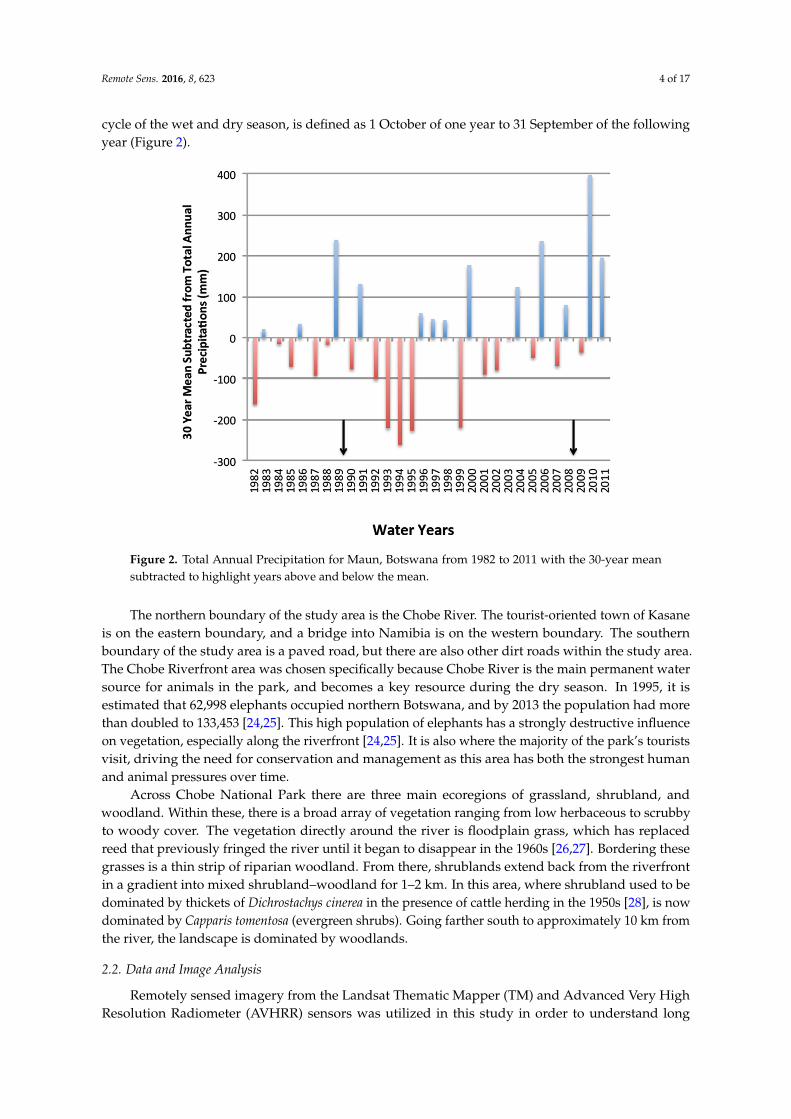
cycle of the wet and dry season, is defined as 1 October of one year to 31 September of the followingyear (Figure 2).Remote Sens. 2016, 8, 623 4 of 16

Figure 2. Total Annual Precipitation for Maun, Botswana from 1982 to 2011 with the 30-year mean subtracted to highlight years above and below the mean.

The northern boundary of the study area is the Chobe River. The tourist-oriented town of Kasane is on the eastern boundary, and a bridge into Namibia is on the western boundary. The southern boundary of the study area is a paved road, but there are also other dirt roads within the study area. The Chobe Riverfront area was chosen specifically because Chobe River is the main permanent water source for animals in the park, and becomes a key resource during the dry season. In 1995, it is estimated that 62,998 elephants occupied northern Botswana, and by 2013 the population had more than doubled to 133,453 [24,25]. This high population of elephants has a strongly destructive influence on vegetation, especially along the riverfront [24,25]. It is also where the majority of the park’s tourists visit, driving the need for conservation and management as this area has both the strongest human and animal pressures over time.

Across Chobe National Park there are three main ecoregions of grassland, shrubland, and woodland. Within these, there is a broad array of vegetation ranging from low herbaceous to scrubby to woody cover. The vegetation directly around the river is floodplain grass, which has replaced reed that previously fringed the river until it began to disappear in the 1960s [26,27]. Bordering these grasses is a thin strip of riparian woodland. From there, shrublands extend back from the riverfront in a gradient into mixed shrubland–woodland for 1–2 km. In this area, where shrubland used to be dominated by thickets of Dichrostachys cinerea in the presence of cattle herding in the 1950s [28], is now dominated by Capparis tomentosa (evergreen shrubs). Going farther south to approximately 10 km from the river, the landscape is dominated by woodlands.

2.2. Data and Image Analysis

Remotely sensed imagery from the Landsat Thematic Mapper (TM) and Advanced Very High Resolution Radiometer (AVHRR) sensors was utilized in this study in order to understand long term trends in vegetation cover and to complete discrete land cover classification with high spatial resolution, embedded within a coarser spatial resolution analysis of monthly NDVI change from AVHRR data. The Landsat data (bands 1–7), used in the multi-date classification, have a 30 m spatial resolution, whereas the AVHRR is much more coarse at 8 km. The Landsat imagery was obtained from Google Earth Engine, but the original data are part of the USGS Landsat catalog. These images

Figure 2. Total Annual Precipitation for Maun, Botswana from 1982 to 2011 with the 30-year meansubtracted to highlight years above and below the mean.

The northern boundary of the study area is the Chobe River. The tourist-oriented town of Kasaneis on the eastern boundary, and a bridge into Namibia is on the western boundary. The southernboundary of the study area is a paved road, but there are also other dirt roads within the study area.The Chobe Riverfront area was chosen specifically because Chobe River is the main permanent watersource for animals in the park, and becomes a key resource during the dry season. In 1995, it isestimated that 62,998 elephants occupied northern Botswana, and by 2013 the population had morethan doubled to 133,453 [24,25]. This high population of elephants has a strongly destructive influenceon vegetation, especially along the riverfront [24,25]. It is also where the majority of the park’s touristsvisit, driving the need for conservation and management as this area has both the strongest humanand animal pressures over time.

Across Chobe National Park there are three main ecoregions of grassland, shrubland, andwoodland. Within these, there is a broad array of vegetation ranging from low herbaceous to scrubbyto woody cover. The vegetation directly around the river is floodplain grass, which has replacedreed that previously fringed the river until it began to disappear in the 1960s [26,27]. Bordering thesegrasses is a thin strip of riparian woodland. From there, shrublands extend back from the riverfrontin a gradient into mixed shrubland–woodland for 1–2 km. In this area, where shrubland used to bedominated by thickets of Dichrostachys cinerea in the presence of cattle herding in the 1950s [28], is nowdominated by Capparis tomentosa (evergreen shrubs). Going farther south to approximately 10 km fromthe river, the landscape is dominated by woodlands.

2.2. Data and Image Analysis

Remotely sensed imagery from the Landsat Thematic Mapper (TM) and Advanced Very HighResolution Radiometer (AVHRR) sensors was utilized in this study in order to understand long

Remote Sens. 2016, 8, 623 5 of 17

term trends in vegetation cover and to complete discrete land cover classification with high spatialresolution, embedded within a coarser spatial resolution analysis of monthly NDVI change fromAVHRR data. The Landsat data (bands 1–7), used in the multi-date classification, have a 30 m spatialresolution, whereas the AVHRR is much more coarse at 8 km. The Landsat imagery was obtainedfrom Google Earth Engine, but the original data are part of the USGS Landsat catalog. These imagescame atmospherically and geometrically corrected, as well as mosaicked together from Google EarthEngine. A pixel-by-pixel composite using the “Simple Landsat Composite Tool” of the study area wasmade of each of the wet and dry season images that had the lowest cloud cover from the 1989–1990and 2008–2009 water years (1 October–30 September). The AVHRR time series imagery was obtainedfrom the GIMMS3g (Global Inventory Monitoring and Modeling System, third generation) NDVI datathat were generated by NASA. The data are available from July 1981 through December 2011, withan 8 km spatial resolution and a 15-day repeat time, which was compiled to create a maximum valuecomposite for each month. The monthly repeat time enables us to detect trends in phenology and totalproductivity for our time period of interest, for 1982–2011.

For the classification analysis based on the composite Landsat data, all of the raw image bands,for both the wet and dry season imagery were included in the classification. In addition a numberof additional layers were created for inclusion in the analysis. For both the Landsat classifier andthe AVHRR time series the NDVI, one of the most commonly used indices, was calculated [29–31].NDVI is a strong indicator of vegetation productivity [32,33] and has been used to study landscapedegradation [34]. In this landscape, the NDVI values ranged from ´0.4 to 0.4, making it an appropriatetechnique for this area because the numbers did not saturate. This index has been heavily usedacross savanna type landscapes with strong results in terms of linkages between NDVI values andvegetation health and productivity [35]. A Tasseled Cap Analysis (TCA) was performed on eachLandsat image to extract Brightness, Greenness, and Wetness variables. In addition, a PrincipleComponents Analysis (PCA) Forward Rotation was also run on the Landsat imagery and the bandsfor components 1, 2, and 3 (which explain over 95% of the variance in the image) were extracted.

2.2.1. Land Cover Classes

According to the literature, the dominant land covers found in the Chobe Riverfront areshrublands, woodlands, and grasslands (which in the dry season will appear as the “bare” cover).Grasslands were defined as non-woody vegetation but also included areas of floodplain vegetationand also soil depending upon the acquisition time of the image. Shrublands were defined as woodyvegetation less than 3 m tall, and woodlands were defined as woody vegetation over 3 m tall. Phenologyof savannas presents another challenge in trying to classify images. In southern Africa, the rainyseason lasts from November to April. Due to the phenology of these systems, ideally for classificationpurposes, both a wet season image and a dry season image across the same water year should be usedto create a single date classification representative of that overall “water year”. Image years closest tothe mean precipitation years were used in order to control for climatic variability and to prevent theuse of an anomalous climatic year—potentially leading to erroneous conclusions on land cover change.

2.2.2. Field/Training Data

Training samples were acquired from two primary sources: field data from the summer of 2009(during the dry season), and Google Earth high-resolution imagery from 2009 (also during the dryseason). In the field, transects were collected along roads due to limited access off-roading in thePark. There were 373 points in total across three broad vegetation types: grassland (62), shrubland(94), and woodland (217). These sample numbers are in accordance with their relative abundancesacross the landscape. The spectral signatures of the spectral bands at each of the training points fromthe 2008–2009 and the 1989–1990 images were graphed in order to check for outliers and consistencywithin class types.

Remote Sens. 2016, 8, 623 6 of 17

A number of different classification techniques were used to allow statistical comparison. In orderto ensure accurate comparison, the same image products were used for all image classifications.In addition, the same set of training sites was used for training and testing. Part of the datasetwas used in the creation of the class signatures for each of the classifications (298 points or 80% ofthe samples-training) and the other part of the dataset was held in reserve for use in the accuracyassessment (75 points or 20% of the training samples-testing). In this manner, there was completecontrol of all data such that a true comparison of techniques was possible. All of the land covertypes listed above were extracted at each of the training sample points to be used in the classification.These were randomly split by the Random Forest model.

2.3. Methods

2.3.1. NDVI Accumulation and Trends

Prior to classification, a NDVI accumulation analysis was conducted to look at long-term trendsacross the landscape. One of the major objections to discrete multi-date classifications is that it is notrepresentative of temporal dynamics and change across the landscape. With this accumulation analysiswe can address the trends in greenness, but not vegetation structural groups. This NDVI analysisutilized zonally averaged pixel-by-pixel AVHRR NDVI data across the entire study area, independentof land cover type. Using R (package: dplyr), the NDVI values were cumulatively summed intwo different ways: (1) across all months and all years; and (2) by season and across all months.The seasonal accumulation utilized the southern hemisphere seasons with summer (DJF: December,January, and February), autumn (MAM: March, April, and May), winter (JJA: June, July, and August),and spring (SON: September, October, and November). For the seasonal accumulation, the NDVIvalues for each season are summed (maximum value of 3 for each season) for each year (maximumvalue of 87 per season over time). This seasonally summed NDVI data were then cumulativelysummed across the time series. By looking at the accumulation rates we can see if greenness valueswere steady over time, similar to a 1:1 line, or if the slope changed indicating changing patterns ofgreenness over time.

2.3.2. Classification Techniques

The most common technique used to monitor land-cover change is through the use of imageclassification. There are a multitude of different types of classifications methods used in mapping landcover with remotely sensed data. Some of the more common methods are supervised classificationsusing algorithms such as maximum likelihood, which assumes that the statistics for each class arenormally distributed and then calculates the probability that a certain pixel belongs in a certainclass [36,37]. In this study, our data do not meet the requirements of normality, and therefore MaximumLikelihood is an inappropriate classifier.

Recently, efficient and accurate machine-learning algorithms have been developed and appliedmore so than traditional parametric algorithms, especially in the case of large and complicated dataand mapping large areas [38–40]. The reason that these algorithms are more efficient and effective isbecause they do not assume normal data distributions, unlike other statistical methods.

Random Forest is one type of machine-learning algorithm, which allows the use of anon-traditional classifier for nonparametric testing with many variables for which it will producethe most important variables for prediction as an output. This ensemble learning technique hasbeen applied in land-cover classifications though multi-spectral imagery [41,42]. The accuracy ofthe classification of this technique may be greater than traditional classifications because it growsan ensemble of statistical trees and they in turn “vote” for the most popular class [43]. This allowsone to use a wide variety of variables of any type. Any variable that needs to be tested for relevancecan be added to the model and the Random Forest will highlight the most important covariates.The pseudo random number generator was seeded with the same number every year the model

Remote Sens. 2016, 8, 623 7 of 17

was run. The model can start out by having 1000 trees; it may be found that a lesser number oftrees are sufficient after running the model. The “mtry”, which is the number of variables randomlysampled as candidates at each split, should be calculated by taking the square root of the number ofcovariates [43]. In this study, the square root of 28 covariates (14 covariates per season) is equal to 5.29,or approximately 5. Other constraints can be optionally added to the model and then it can be run.One of the greatest advantages of Random Forest is that it does not overfit the data because with thelarge number of trees, there is a low generalization error [43]. This technique is not yet widely used,but it seems ideal for remote sensing classification, especially in heterogeneous landscapes such as thecomplex, temporally and spatially constrained, savanna landscapes of Southern Africa. An additionalbenefit of using the Random Forest classification is that you can obtain several measures of variableimportance including Mean Decrease in Accuracy and the Mean Decrease in Gini coefficient, whichcan then be used to aid in image classification.

3. Results

3.1. Cumulative NDVI

The greening trends across the Chobe riverfront showed no sharp or rapid changes in greenness.The accumulations, both total and seasonal, illustrate that while there is variability in NDVI acrosstime there were no major breakpoints. The total NDVI accumulation across all months and all years(Figure 3b) showed a consistent increase with no large change in slope; meaning that the cumulativesummation for the most part followed that 1:1 line, with only a slight divergence in the later portionof the time series. Figure 3a shows the trends in NDVI by season across the study area. The DJFseason throughout the time series has the highest NDVI. This is the wet season in this study areaand a time of great vegetation flush. The wet season continues into March, ending around late Aprilto early May. The NDVI seasonal summation shows that the MAM season has the second highestin production. The dry season in the study area runs through the JJA season and the SON season,resulting in the lowest NDVI summations. However, the JJA season has higher NDVI accumulation,as woody vegetation stays green late into the dry season. Figure 3 also highlights that the years ofselection for the land cover classifications: 1989–1990 and 2008–2009 are not in any way anomalousyears either seasonally or across the full water year.

Remote Sens. 2016, 8, 623 7 of 16

of using the Random Forest classification is that you can obtain several measures of variable importance including Mean Decrease in Accuracy and the Mean Decrease in Gini coefficient, which can then be used to aid in image classification.

3. Results

3.1. Cumulative NDVI

The greening trends across the Chobe riverfront showed no sharp or rapid changes in greenness. The accumulations, both total and seasonal, illustrate that while there is variability in NDVI across time there were no major breakpoints. The total NDVI accumulation across all months and all years (Figure 3b) showed a consistent increase with no large change in slope; meaning that the cumulative summation for the most part followed that 1:1 line, with only a slight divergence in the later portion of the time series. Figure 3a shows the trends in NDVI by season across the study area. The DJF season throughout the time series has the highest NDVI. This is the wet season in this study area and a time of great vegetation flush. The wet season continues into March, ending around late April to early May. The NDVI seasonal summation shows that the MAM season has the second highest in production. The dry season in the study area runs through the JJA season and the SON season, resulting in the lowest NDVI summations. However, the JJA season has higher NDVI accumulation, as woody vegetation stays green late into the dry season. Figure 3 also highlights that the years of selection for the land cover classifications: 1989–1990 and 2008–2009 are not in any way anomalous years either seasonally or across the full water year.

Figure 3. Cumulative NDVI (Normalized Difference Vegetation Index) across the AVHRR (Advanced Very High Resolution Radiometer) time series (1982–2011): (a) accumulated per season, but not across years; and (b) accumulated per season and across years.

3.2. Random Forest Classification

One of the most important products of the Random Forest classification was a land cover map of Chobe National Park across both dates (Figure 4). These maps show the grassland, shrubland, and woodland classes across the landscape. Other types of traditional supervised classification techniques result in high confusion in the shrubland class—which can be expected in these savanna systems because they can be spectrally similar to other classes as we divided them by their height difference. Of interest then is whether the increased complexity of the Random Forest classifier allows for any improvement in classification accuracy when the identical training data and accuracy assessment data are used within the model. Random Forest proved to have superior statistical power in this analysis. The overall accuracy of the Random Forest classifier was the highest of the classifiers tested,

SON MAM JJA DJF

Year

Year

a)

b)

Figure 3. Cumulative NDVI (Normalized Difference Vegetation Index) across the AVHRR (AdvancedVery High Resolution Radiometer) time series (1982–2011): (a) accumulated per season, but not acrossyears; and (b) accumulated per season and across years.

Remote Sens. 2016, 8, 623 8 of 17

3.2. Random Forest Classification

One of the most important products of the Random Forest classification was a land cover map ofChobe National Park across both dates (Figure 4). These maps show the grassland, shrubland, andwoodland classes across the landscape. Other types of traditional supervised classification techniquesresult in high confusion in the shrubland class—which can be expected in these savanna systemsbecause they can be spectrally similar to other classes as we divided them by their height difference.Of interest then is whether the increased complexity of the Random Forest classifier allows for anyimprovement in classification accuracy when the identical training data and accuracy assessment dataare used within the model. Random Forest proved to have superior statistical power in this analysis.The overall accuracy of the Random Forest classifier was the highest of the classifiers tested, at 79.8%for 1989–1990 and 78.5% for 2008–2009 (Table 1). Results from the other classifiers include the minimumdistance to means (53% in 1989–1990 and 72% in 2008–2009) and parallelepiped (67% for 1989–1990 and72% for 2008–2009). The error matrix (Table 1) shows that misclassification, and therefore a decrease inclassification accuracy, occurred mostly in the shrubland class. This is because it is a difficult class todiscern. Shrublands often represent the same species as the woodland class, but are shorter (less than3 m in height) and so spectrally have the most confusion. The confusion with the woodland andshrubland classes is therefore understandable, although the Random Forest classifier does the bestdifferentiation overall.

Remote Sens. 2016, 8, 623 8 of 16

at 79.8% for 1989–1990 and 78.5% for 2008–2009 (Table 1). Results from the other classifiers include the minimum distance to means (53% in 1989–1990 and 72% in 2008–2009) and parallelepiped (67% for 1989–1990 and 72% for 2008–2009). The error matrix (Table 1) shows that misclassification, and therefore a decrease in classification accuracy, occurred mostly in the shrubland class. This is because it is a difficult class to discern. Shrublands often represent the same species as the woodland class, but are shorter (less than 3 m in height) and so spectrally have the most confusion. The confusion with the woodland and shrubland classes is therefore understandable, although the Random Forest classifier does the best differentiation overall.

Figure 4. Random Forest classification results based on the Landsat imagery for: (a) 1989–1990; and (b) 2008–2009 image series.

Table 1. Error Matrix for Random Forest classification results based on the Landsat imagery for 1989–1990 and 2008–2009 image series.

Error Matrix

Woodland Shrub Land

Grassland Total Class Error Omission %

Class Error Commission %

1989–1990Woodland 165 13 3 181 8.84 14.9 Shrubland 24 36 6 66 45.5 37.9 Grassland 5 9 36 50 27.5 19.6

Total 194 58 45 297 2008–2009

Woodland 161 17 3 181 11.0 15.3 Shrubland 24 36 6 66 45.5 41.9 Grassland 5 9 37 51 27.5 19.6

Total 190 62 46 298 Kappa Coefficient: 0.6237 Overall Accuracy: 79.9%; Kappa Coefficient: 0.6025 Overall Accuracy: 78.5%.

Figure 4. Random Forest classification results based on the Landsat imagery for: (a) 1989–1990; and(b) 2008–2009 image series.

Remote Sens. 2016, 8, 623 9 of 17

Table 1. Error Matrix for Random Forest classification results based on the Landsat imagery for1989–1990 and 2008–2009 image series.

Error Matrix Woodland Shrub Land Grassland Total Class ErrorOmission %

Class ErrorCommission %

1989–1990

Woodland 165 13 3 181 8.84 14.9Shrubland 24 36 6 66 45.5 37.9Grassland 5 9 36 50 27.5 19.6

Total 194 58 45 297

2008–2009

Woodland 161 17 3 181 11.0 15.3Shrubland 24 36 6 66 45.5 41.9Grassland 5 9 37 51 27.5 19.6

Total 190 62 46 298

Kappa Coefficient: 0.6237 Overall Accuracy: 79.9%; Kappa Coefficient: 0.6025 Overall Accuracy: 78.5%.

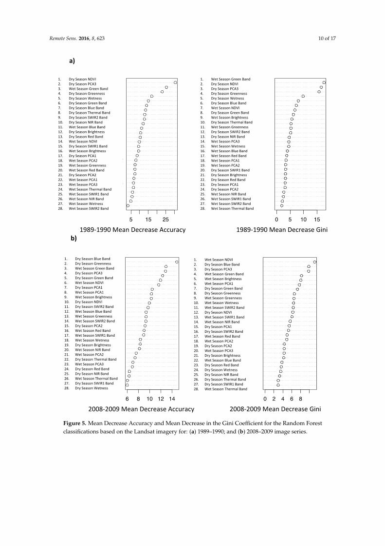
An additional strength of the Random Forest classifier, when compared to the more traditionalsupervised classification techniques comes from the relative influence plots (Figure 5), which allow usto determine the importance of each of the covariates within the analysis. The importance of usingboth the wet season and the dry season imagery is evident—with different covariates from both beingpulled into the analysis as the most important variables, making the results more robust (Figure 5).The 1989–1990 classification (Figure 5a) has wet season green band, dry season NDVI, dry season PCABand 3, and dry season TCA bands 2 (greenness) and 3 (moisture) as the most important covariates inthe model. These variables are readily explained, in terms of their top selection by the model becausethey are the variables associated with vegetation health and vigor. For 2008–2009 (Figure 5b), dryseason blue band, dry season PCA band 3, wet season NDVI, dry and wet season green bands, dryseason TCA greenness, wet season TCA brightness and wet season PCA component 1 are the mostimportant covariates in the model. Again both dry and wet season variables are selected as importantand although in differing order of importance the NDVI, TCA, PCA component 3 and green bandsare all key. Again these variables do suggest the vigor and health of vegetation being the dominantcover to discern. Interestingly, the same bands are not selected in the same order and some trends varyacross dates, although once the extent of the change in vegetation cover is seen (Figure 6) we can seethat more soil based indices and bands are selected in 2008–2009, as these are more dominant in thedry season imagery for this date, due in part to the land cover changes which have occurred acrossthe two composite image dates. This certainly highlights the importance of including both dry andwet season images within the study and classification of land cover, and also highlights some of thevalue of the Random Forest classifier, when interpretation of the selected variables can be discussedand explained. The Mean Decrease in Accuracy shows the Mean Squared Error when the variableis randomly permuted in the model, and the Mean Decrease in Gini is an impurity criterion, whichshows when a particular predictor variable played a larger role in partitioning the data that definedthe classes. These two measures are often consistent.

Remote Sens. 2016, 8, 623 10 of 17

Remote Sens. 2016, 8, 623 9 of 16

An additional strength of the Random Forest classifier, when compared to the more traditional supervised classification techniques comes from the relative influence plots (Figure 5), which allow us to determine the importance of each of the covariates within the analysis. The importance of using both the wet season and the dry season imagery is evident—with different covariates from both being pulled into the analysis as the most important variables, making the results more robust (Figure 5). The 1989–1990 classification (Figure 5a) has wet season green band, dry season NDVI, dry season PCA Band 3, and dry season TCA bands 2 (greenness) and 3 (moisture) as the most important covariates in the model. These variables are readily explained, in terms of their top selection by the model because they are the variables associated with vegetation health and vigor. For 2008–2009 (Figure 5b), dry season blue band, dry season PCA band 3, wet season NDVI, dry and wet season green bands, dry season TCA greenness, wet season TCA brightness and wet season PCA component 1 are the most important covariates in the model. Again both dry and wet season variables are selected as important and although in differing order of importance the NDVI, TCA, PCA component 3 and green bands are all key. Again these variables do suggest the vigor and health of vegetation being the dominant cover to discern. Interestingly, the same bands are not selected in the same order and some trends vary across dates, although once the extent of the change in vegetation cover is seen (Figure 6) we can see that more soil based indices and bands are selected in 2008–2009, as these are more dominant in the dry season imagery for this date, due in part to the land cover changes which have occurred across the two composite image dates. This certainly highlights the importance of including both dry and wet season images within the study and classification of land cover, and also highlights some of the value of the Random Forest classifier, when interpretation of the selected variables can be discussed and explained. The Mean Decrease in Accuracy shows the Mean Squared Error when the variable is randomly permuted in the model, and the Mean Decrease in Gini is an impurity criterion, which shows when a particular predictor variable played a larger role in partitioning the data that defined the classes. These two measures are often consistent.

Remote Sens. 2016, 8, 623 10 of 16

Figure 5. Mean Decrease Accuracy and Mean Decrease in the Gini Coefficient for the Random Forest classifications based on the Landsat imagery for: (a) 1989–1990; and (b) 2008–2009 image series.

Figure 6. Land Cover Change Trajectories from 1989–1990 to 2008–2009 for the Random Forest classifier for the Chobe Riverfront.

3.3. Change Trajectory for Random Forest Classification

A land-cover classification change trajectory was then created using the results of the Random Forest classification (Figure 6). The pixel counts and percent change for each of these class conversions is defined in Table 2. This trajectory shows a significant loss of grassland and also trends of woody vegetation conversion along the dirt roads/fire breaks. There was also an increase in woody vegetation along the river on the west side of the Park. The land-cover change trajectory from the Random Forest classifier (Figure 6) produced clear spatial trends of land-cover classes across the

Figure 5. Mean Decrease Accuracy and Mean Decrease in the Gini Coefficient for the Random Forestclassifications based on the Landsat imagery for: (a) 1989–1990; and (b) 2008–2009 image series.

Remote Sens. 2016, 8, 623 11 of 17

Remote Sens. 2016, 8, 623 10 of 16

Figure 5. Mean Decrease Accuracy and Mean Decrease in the Gini Coefficient for the Random Forest classifications based on the Landsat imagery for: (a) 1989–1990; and (b) 2008–2009 image series.

Figure 6. Land Cover Change Trajectories from 1989–1990 to 2008–2009 for the Random Forest classifier for the Chobe Riverfront.

3.3. Change Trajectory for Random Forest Classification

A land-cover classification change trajectory was then created using the results of the Random Forest classification (Figure 6). The pixel counts and percent change for each of these class conversions is defined in Table 2. This trajectory shows a significant loss of grassland and also trends of woody vegetation conversion along the dirt roads/fire breaks. There was also an increase in woody vegetation along the river on the west side of the Park. The land-cover change trajectory from the Random Forest classifier (Figure 6) produced clear spatial trends of land-cover classes across the

Figure 6. Land Cover Change Trajectories from 1989–1990 to 2008–2009 for the Random Forest classifierfor the Chobe Riverfront.

3.3. Change Trajectory for Random Forest Classification

A land-cover classification change trajectory was then created using the results of the RandomForest classification (Figure 6). The pixel counts and percent change for each of these class conversionsis defined in Table 2. This trajectory shows a significant loss of grassland and also trends of woodyvegetation conversion along the dirt roads/fire breaks. There was also an increase in woody vegetationalong the river on the west side of the Park. The land-cover change trajectory from the Random Forestclassifier (Figure 6) produced clear spatial trends of land-cover classes across the region. Directlyalong the riverfront there was a conversion from woodland towards grassland. Just south of that,the dominant conversion was towards shrubland. Woodland is found in the region the furthest backfrom the riverfront. The overall patterns of vegetation cover over the two dates clearly showingan expansion of shrubland at an increasing distance from the river. Some areas of conversion fromshrubland to woodland (woodland growth and aging) also occur farther back from the riverfront,especially along areas of roads and development, which were initiated in the 1970s and 1980s and arekept cut and cleared as part of the park management.

Table 2. Change trajectory percent change from 1989–1990 to 2008–2009 across landscape using theRandom Forest classifier.

Random Forest Classifier (Pixel Count) Random Forest Classifier (% Change)

Woodland to Grassland 6890 1.46Woodland to Shrubland 18,218 3.87

No Change 411,754 87.4Shrubland to Woodland 28,425 6.03Grassland to Woodland 5802 1.23

Total 471,089 99.99

4. Discussion

Based on Vogel and Strohbach’s 2009 definition of degradation, we can clearly state that someforms of degradation are occurring in the Chobe National Park Riverfront. Spatially, we see theconversion from woodland to grassland, or woodland to shrubland (both a loss of woodland) occurring

Remote Sens. 2016, 8, 623 12 of 17

directly along the river and just behind it, which has the most animal and tourist traffic. The primaryconversions in the area away from the river were from shrubland to woodland, and woodland toshrubland (woody conversions). The patterns found in this region match those patterns found acrosssouthern Africa where there has been an increase in woody vegetation (mostly shrubland) and adecrease in grassland [19,20,44]. Degradation of the herbaceous layer in this region began in the 1960sdue to human land use, such as cattle, fire, logging, and agriculture [45].

Remote sensing in savanna landscapes can be a complex pursuit due to the heterogeneous natureof the landscape and possible spectral confusion due to the definition of a shrub versus a tree, which isdetermined solely by height. Ultimately, the Random Forest classifier was the best method for use indifferentiation of the savanna vegetation types. This study was important in testing the Random Forestclassifier in a savanna landscape, where it has only been tested a limited amount thus far. The RandomForest classifier did very well, as evidenced by the accuracy assessments and kappa values, given thecomplex heterogeneous nature of the savanna landscape with overall accuracies close to 80%. In otherlandscapes, studies have shown that the Random Forest classifier consistently outperformed all othertraditional methods tested [42,46,47]. The Random Forest classifier also provided valuable insight asto which variables were significant in creating the classification scheme, which differed across years.This is of key importance in such savanna landscapes, especially for studies using only a single seasonfor analysis, where findings or interpretations based only on one season, might be incorrect. It alsohighlights the dynamic nature of savanna landscapes, both spatially and temporally, again, linkingback to our reason for using this complex classification methodology versus much more static methods,which usually fail to work well in savannas. Classification highlighted the increases in bare land andsoil in the later date and this is seen also in the images highlighted in the analysis.

AVHRR data provide one of the longest remotely sensed datasets currently available. The monthlycomposites based on the maximum 16-day data from 1982-present enable long term landscape levelanalysis to be completed. While the spatial resolution is not as fine as Landsat, the large swath widthallows for landscape to global scale analysis of ecosystem dynamics that are not currently availablewith finer scale data. In this study, the AVHRR data are utilized to understand trends across theentire time series while the Landsat data are used to classify the landscape only at discrete dates.Additionally, the AVHRR time series illustrates the longer-term dynamics within which our discreteLandsat imagery is located. By looking at seasonal NDVI accumulation we can detect deviations in thegreening trends over time. The seasonal NDVI can be viewed as a time series (Figure 3a) or can beconsidered cumulatively (Figure 3b), which is a metric of NDVI, or a proxy for production. We seea weak declining trend across all seasons. The season with the highest NDVI accumulation is DJF,indicative of both the grass and woody component. The season with the lowest NDVI accumulationis SON. Most might think that JJA is the lowest since this is the core of the dry season. However, bythe time SON comes, months of depleted soil moisture have occurred leading to grass brown downand loss of woody vegetation leaves. With the total accumulation (Figure 3b) you can readily see theseasonal effect. The DJF and MAM seasons represent the time of greatest vegetation flush. Typicallythe wet season starts in late boreal autumn (October–November) and with the 4–6 weeks delay fromonset of precipitation to flush that leads to the DJF season.

There have been some distinct vegetation changes in this savanna ecosystem along the ChobeRiverfront between 1989 and 2009. The data show that there are no significant longer-term trends here,e.g., due to precipitation changes or the like, that could influence vegetation. Furthermore, the lackof real trends in precipitation or NDVI show that climate, the major driver of land cover change insavannas, is not the main driving force of change here, but rather people, management and herbivoryare. In addition, fire is excluded as a major driver due to the extensive fire ban across Botswana. Unlikeacross the border in Namibia, where managers operate on yearly burn cycles, burning for managementhas been banned in Botswana for the last two decades [12]. When natural fires do occur, they aresuppressed and this low fire frequency is also known to contribute to increased bush encroachmentin this landscape [12,13]. So this analysis is also pointing out that the main drivers of change are not

Remote Sens. 2016, 8, 623 13 of 17

fluctuating, but areas on our landscape are. This must then be due to management and people, ormore specifically herbivory and elephants (and lack of control over their numbers, i.e., hunting ban inBotswana and exploding elephant populations over this time period).

Using the Random Forest classifier, the conversion of woodland to grassland and woodland toshrubland directly along the river (Figure 7) is likely linked to an increase in the elephant populationin northern Botswana from an estimated 62,998 in 1995 to 133,453 in 2013 [25]. Through time, asthe elephant population has increased, the amount of degradation in the area has increased withit, especially focused on the riverfront area. Utilization of this area by animals is thought to be oneof the major causes of this degradation [21]. The piosphere effect can be defined as the amount ofelephant debarking, ringing, and knocking down trees increasing with decreasing distance to a watersource [21]. At the scale at which we observe degradation, this study displays the characteristics of thepiosphere effect. This is felt especially in this area because the Chobe River is their main source of water,particularly during the dry season when they utilize this area the most. We also see a conversion fromwoodland to shrubland, shrubland to woodland, and grassland to woodlands happening along roadsback from the river. This change can be explained by the utilization of elephants and Park managersclearing along these tracts inside the Park as narrow roads and firebreaks. There is a dense amountof woodland to shrubland vegetation conversion occurring along the west side of the Park directlyalong the river. Due to the rocky terrain of this area, there are few tourists and therefore degradation isthought to be primarily from usage by animals.Remote Sens. 2016, 8, 623 13 of 16

Figure 7. Photos of the Chobe Riverfront in the dry season, highlighting expanses of bare ground and shrub cover, and lack of larger trees. Photos taken by Jane Southworth.

There are certain biological implications of vegetation conversion. For example, in this region in the 1980s, encroachment of low-quality pioneer shrubland species was later made possible by impalas colonizing these areas, which is enhanced once elephants have opened up the woodlands [24]. The impala prevented higher-quality tree species regeneration [48] through seedling predation [49]. This also impacts the species that could graze in this area. More specialized browsers, such as bushbuck could not survive in this area because the vegetation was converting towards being a monospecies. In turn, less specialized browsers were able to thrive in these areas and continue to drive the vegetation degradation. These non-specialized browsers, such as elephant and giraffe, continue to dominate this area today. It is possible that this shift has reduced the specialized grazers along the riverfront, such as zebra, roan, and waterbuck, having a potential impact on tourism [22].

There are also implications for using the AVHRR data, mainly the coarse spatial resolution. This resolution limits the utility in using AVHRR data for classification and land use/land cover change. Instead, we speak to ecosystem trends measuring events such as degradation and bush encroachment, which have occurred across the savanna landscapes of southern Africa, including Chobe National Park. This park is a vital resource for livelihoods of those residing in the villages surrounding the park. Communities such a Chobe enclave have embraced tourism as a source of livelihood, moving away from traditional sources of development, namely agriculture. By utilizing both AVHRR and Landsat data we can monitor the resilience, drivers, and importantly land cover of this vital national park.

A concern about the class system utilized is that the difference in definition between shrubland and woodland is defined by height, a common practice in savanna where a tree versus a shrubland of the same species, is simply a function of plant height. Therefore, these can be difficult to differentiate using spectral data. This may be why we are seeing an increase from shrubland to woodland in some small areas, and explain why there was the most confusion within the shrubland class. Between these two image dates, the class that is a conversion from shrubland to woodland may be a growth in height of these species, as well as a replacement of naturally occurring woodlands to lower-quality shrubland/tree species, such as Croton megalobotrys [22].

Figure 7. Photos of the Chobe Riverfront in the dry season, highlighting expanses of bare ground andshrub cover, and lack of larger trees. Photos taken by Jane Southworth.

There are certain biological implications of vegetation conversion. For example, in this regionin the 1980s, encroachment of low-quality pioneer shrubland species was later made possible byimpalas colonizing these areas, which is enhanced once elephants have opened up the woodlands [24].The impala prevented higher-quality tree species regeneration [48] through seedling predation [49].This also impacts the species that could graze in this area. More specialized browsers, such as bushbuckcould not survive in this area because the vegetation was converting towards being a monospecies.

Remote Sens. 2016, 8, 623 14 of 17

In turn, less specialized browsers were able to thrive in these areas and continue to drive the vegetationdegradation. These non-specialized browsers, such as elephant and giraffe, continue to dominate thisarea today. It is possible that this shift has reduced the specialized grazers along the riverfront, such aszebra, roan, and waterbuck, having a potential impact on tourism [22].

There are also implications for using the AVHRR data, mainly the coarse spatial resolution. Thisresolution limits the utility in using AVHRR data for classification and land use/land cover change.Instead, we speak to ecosystem trends measuring events such as degradation and bush encroachment,which have occurred across the savanna landscapes of southern Africa, including Chobe NationalPark. This park is a vital resource for livelihoods of those residing in the villages surrounding the park.Communities such a Chobe enclave have embraced tourism as a source of livelihood, moving awayfrom traditional sources of development, namely agriculture. By utilizing both AVHRR and Landsatdata we can monitor the resilience, drivers, and importantly land cover of this vital national park.

A concern about the class system utilized is that the difference in definition between shrublandand woodland is defined by height, a common practice in savanna where a tree versus a shrubland ofthe same species, is simply a function of plant height. Therefore, these can be difficult to differentiateusing spectral data. This may be why we are seeing an increase from shrubland to woodland in somesmall areas, and explain why there was the most confusion within the shrubland class. Betweenthese two image dates, the class that is a conversion from shrubland to woodland may be a growth inheight of these species, as well as a replacement of naturally occurring woodlands to lower-qualityshrubland/tree species, such as Croton megalobotrys [22].

5. Conclusions

The research presented here addresses issues of key concern in dryland ecosystems—that ofmonitoring change across landscapes where definitions of land cover classes merely rely on a count orheight of trees versus shrubs. Traditionally, remote sensing has failed to classify such landscapes welland this work presented some new techniques to incorporate these discrete land cover changes—usingRandom Forest classification approaches—within a more continuous view of the landscapes—asimpacted by temporal variability due to precipitation and other drivers. Using the continuous NDVIanalysis helps position our study in a broader context and also addresses climate variability as apotential driver of change (most savanna landscapes are very sensitive to precipitation). This analysisincorporates the larger trends of the landscape and accounts for such changes in climate, and only thenaddresses the discrete classification approach, used more traditionally outside of dryland savannasystems. Our findings as presented highlight the success of the approach and the importance oflooking at both temporal trends and spatial patterns when studying such systems, and especially whenmanagement must address such processes of vegetation change and conversion, degradation and oftenwildlife management, within the temporal and spatial matrix that makes up their park landscape.

The findings of this study could have significant implications for management and impact tourismin the park, given the main areas of degradation are along the main tourist routes and the riverfront.The changing vegetation could lead to a change in elephant usage of the landscape, and therefore theareas and frequency in which tourists can view the wildlife. In the future, habitat classification couldbe improved by monitoring more image dates, using finer spatial resolution imagery, and conductingmore fieldwork for validation—linking changes directly to vegetation plot work and species.

Acknowledgments: The authors would like to thank those who edited this paper and offered external guidance.This includes Tim Fullman, who was responsible for providing the training sample points and GIS data for ChobeNational Park, and Alassane Barro, who was responsible for ensuring that the R code was creating maps.

Author Contributions: Hannah Herrero was responsible for running the Random Forest analysis and writingthe paper. Jane Southworth was responsible for creating the research design and editing. Erin Bunting wasresponsible for obtaining the Landsat images, setting up the Random Forest code, and completing the NDVIaccumulation analysis.

Conflicts of Interest: The authors declare no conflict of interest.

Remote Sens. 2016, 8, 623 15 of 17

References

1. Vitousek, P.M.; Mooney, H.A.; Lubchenco, J.; Melillo, J.M. Human domination of earth’s ecosystems. Science1997, 277, 494–499. [CrossRef]

2. Pielke, R.A. Land use and climate change. Science 2005, 310, 1625–1626. [CrossRef] [PubMed]3. Turner, B.L., II; Kasperson, R.E.; Meyer, W.B.; Dow, K.M.; Golding, D.; Kasperson, J.X.; Mitchell, R.C.;

Ratick, S.J. Two types of global environmental change: Definitional and spatial-scale issues in their humandimensions. Glob. Environ. Chang. 1990, 1, 14–22. [CrossRef]

4. Chapin, F.S., III; Chapin, M.C.; Matson, P.A.; Vitousek, P. Principles of Terrestrial Ecosystem Ecology; Springer:Berlin, Germany; Heidelberg, Germany, 2011.

5. Scholes, R.J.; Archer, S.R. Tree-grass interactions in savannas. Ann. Rev. Ecol. Syst. 1997, 28, 517–544.[CrossRef]

6. Hanan, N.; Lehmann, C. Tree-Grass Interactions in Savannas: Paradigms, Contradictions, and Conceptual Models;Taylor and Francis Group: Boca Raton, FL, USA, 2010.

7. Scholes, R.J.; Walker, B.H. An African Savanna: Synthesis of the Nylsvley Study; Cambridge University Press:Cambridge, UK, 1993.

8. Sprugel, D.G. Disturbance, equilibrium, and environmental variability: What is ‘natural’ vegetation in achanging environment? Biol. Conserv. 1991, 58, 1–18. [CrossRef]

9. Vogel, M.; Strohbach, M. Monitoring of savanna degradation in Namibia using Landsat TM/ETM+ data.In Proceedings of the IEEE International Geoscience and Remote Sensing Symposium, Cape Town, SouthAfrica, 12–17 July 2009.

10. Andela, N.; Liu, Y.Y.; van Dijk, A.I.J.M.; de Jeu, R.A.M.; McVicar, T.R. Global changes in dryland vegetationdynamics (1988–2008) assessed by satellite remote sensing: Comparing a new passive microwave vegetationdensity record with reflective greenness data. Biogeosciences 2013, 10, 6657–6676. [CrossRef]

11. Campo-Bescós, M.A.; Muñoz-Carpena, R.; Southworth, J.; Zhu, L.; Waylen, P.R.; Bunting, E. Combinedspatial and temporal effects of environmental controls on long-term monthly NDVI in the Southern Africasavanna. Remote Sens. 2013, 5, 6513–6538. [CrossRef]

12. Pricope, N.G.; Binford, M.W. A Spatio-temporal analysis of fire recurrence and extent for semi-arid savannaecosystems in Southern Africa using moderate-resolution satellite imagery. J. Environ. Manag. 2012, 100,72–85. [CrossRef] [PubMed]

13. Moleele, N.M.; Ringrose, S.; Matheson, W.; Vanderpost, C. More woody plants? The status of bushencroachment in Botswana’s Grazing Areas. J. Environ. Manag. 2002, 64, 3–11. [CrossRef]

14. Vidal, J. Botswana Bushmen: If You Deny Us the Right to Hunt, You Are Killing Us. Availableonline: http://www.theguardian.com/environment/2014/apr/18/kalahari-bushmen-hunting-ban-prince-charles (accessed on 19 February 2016).

15. Archer, S.; Schimel, D.S.; Holland, E.A. Mechanisms of shrubland expansion: Land use, climate or CO2?Clim. Chang. 1995, 29, 91–99. [CrossRef]

16. Van Auken, O.W. Shrub invasions of North American semiarid grasslands. Annu. Rev. Ecol. Syst. 2000, 31,197–215. [CrossRef]

17. Bond, W.J.; Midgley, G.F.; Woodward, F.I. The importance of low atmospheric CO2 and fire in promoting thespread of grasslands and savannas. Glob. Chang. Biol. 2003, 9, 973–982. [CrossRef]

18. Asner, G.P.; Elmore, A.J.; Olander, L.P.; Martin, R.E.; Harris, A.T. Grazing systems, ecosystem responses, andglobal change. Annu. Rev. Environ. Resour. 2004, 29, 261–299.

19. Campbell, A.; Child, G. The impact of man on the environment of Botswana. Botsw. Notes Rec. 1971, 3,91–110.

20. Ringrose, S.; Matheson, W.; Wolski, P.; Huntsman-Mapila, P. Vegetation cover trends along the BotswanaKalahari Transect. J. Arid Environ. 2008, 54, 297–317. [CrossRef]

21. Fullman, T.J.; Child, B. Water distribution at local and landscape scales affects tree utilization by elephants inChobe National Park, Botswana. Afr. J. Ecol. 2013, 51, 235–243. [CrossRef]

22. Wolf, A. Preliminary Assessment of the Effect of High Elephant Density on Ecosystem Components(Grass, Trees, and Large Mammals) on the Chobe Riverfront in Northern Botswana. Master’s Thesis,University of Florida, Gainesville, FL, USA, 2009.

Remote Sens. 2016, 8, 623 16 of 17

23. Sankaran, M.; Hanan, N.P.; Scholes, R.J.; Ratnam, J.; Augustine, D.J.; Cade, B.S.; Gignoux, J.; Higgins, S.I.; LeRoux, X.; Ludwig, F.; et al. Determinants of woody cover in African savannas. Nature 2005, 438, 846–849.[CrossRef] [PubMed]

24. Mosugelo, D.K.; Moe, S.R.; Ringrose, S.; Nellemann, C. Vegetation changes during a 36-year period inNorthern Chobe National Park, Botswana. Afr. J. Ecol. 2002, 40, 232–240. [CrossRef]

25. African Elephant Database. Available online: http://www.elephantdatabase.org/ (accessed on19 February 2016).

26. Henry, F.W.T. Enumeration Report of the Chobe Main Forest Block; Ministry of Agriculture: Gaborone,Botswana, 1966.

27. Selous, F.C. A Hunter’s Wanderings in Africa: Being a Narrative of Nine Years Spent Amongst the Game of the FarInterior of South Africa; R. Bentley & Son: London, UK, 1881.

28. Child, G.E.T. An Ecological Survey of North-Eastern Botswana; Report No. TA2563; FAO: Rome, Italy, 1968.29. Rouse, J.W., Jr. Monitoring the Vernal Advancement and Retrogradation (Green Wave Effect) of Natural Vegetation;

Texas A & M University, Remote Sensing Center: College, TX, USA, 1973.30. Tucker, C.J. Red and Photographic Infrared Linear Combinations for Monitoring Vegetation. Remote Sens. Environ.

1979, 8, 127–150. [CrossRef]31. Beck, H.E.; McVicar, T.R.; van Dijk, A.I.J.M.; Schellekens, J.; de Jeu, R.A.M.; Bruijnzeel, L.A. Global

Evaluation of four AVHRR–NDVI data sets: Intercomparison and assessment against Landsat imagery.Remote Sens. Environ. 2011, 115, 2547–2563. [CrossRef]

32. Tucker, C.J.; Townshend, J.R.G.; Goff, T.E. African land-cover classification using satellite data. Science 1985,227, 369–375. [CrossRef] [PubMed]

33. McVicar, T.R.; Jupp, D.L.B. The current and potential operational uses of remote sensing to aid decisions ondrought exceptional circumstances in Australia: A review. Drought Policy Assess. Declar. 1998, 57, 399–468.[CrossRef]

34. Bai, Z.G.; Dent, D.L.; Olsson, L.; Schaepman, M.E. Proxy global assessment of land degradation.Soil Use Manag. 2008, 24, 223–234. [CrossRef]

35. Fung, T.; Siu, W. Environmental quality and its changes, an analysis using NDVI. Int. J. Remote Sens. 2010,21, 1011–1024. [CrossRef]

36. Jensen, J.R. Introductory Digital Image Processing, 3rd ed.; Prentice Hall: Upper Saddle River, NJ, USA, 2005.37. Maximum Likelihood Supervised Classification. Available online: http://www.exelisvis.com/docs/

MaximumLikelihood.html (accessed on 19 February 2016).38. Hansen, M.; Dubayah, R.; Defries, R. Classification trees: An alternative to traditional land cover classifiers.

Int. J. Remote Sens. 1996, 17, 1075–1081. [CrossRef]39. Huang, C.; Davis, L.S.; Townshend, J.R.G. An Assessment of support vector machines for land cover

classification. Int. J. Remote Sens. 2002, 23, 725–749. [CrossRef]40. Rogan, J.; Miller, J.; Stow, D.; Franklin, J.; Levien, L.; Fischer, C. Land-cover change monitoring with

classification trees using Landsat TM and ancillary data. Photogramm. Eng. Remote Sens. 2003, 69, 793–804.[CrossRef]

41. Fan, H. Land-cover mapping in the Nujiang Grand Canyon: Integrating spectral, textural, and topographicdata in a random forest classifier. Int. J. Remote Sens. 2013, 34, 7545–7567. [CrossRef]

42. Gislason, P.O.; Benediktsson, J.A.; Sveinsson, J.R. Random forests for land cover classification.Pattern Recognit. Remote Sens. 2006, 27, 294–300. [CrossRef]

43. Breiman, L. Random forests. Mach. Learn. 2001, 45, 5–32. [CrossRef]44. Robert, A.M.; Tchebakova, N.M.; Leemans, R. Global vegetation change predicted by the modified Budyko

model. Clim. Chang. 1993, 25, 59–83.45. Kelly, R.D.; Walker, B.H. The effects of different forms of land use on the ecology of a semi-arid region in

South-Eastern Rhodesia. J. Ecol. 1976, 64, 553–576. [CrossRef]46. Pal, M. Random Forest classifier for remote sensing classification. Int. J. Remote Sens. 2005, 26, 217–222.

[CrossRef]47. Prasad, A.M.; Iverson, L.R.; Liaw, A. Newer classification and regression tree techniques: Bagging and

random forests for ecological prediction. Ecosystems 2006, 9, 181–199. [CrossRef]

Remote Sens. 2016, 8, 623 17 of 17

48. Rutina, L.P. Impalas in an Elephant-Impacted Woodland: Browser-Driven Dynamics of the Chobe RiparianZone, Northern Botswana. Ph.D. Thesis, Agricultural University of Norway, Akershus, Norway, 2004.

49. Moe, S.R.; Rutina, L.P.; Hytteborn, H.; Toit, J.T.D. What Controls woodland regeneration after elephants havekilled the big trees? J. Appl. Ecol. 2009, 46, 223–230. [CrossRef]

© 2016 by the authors; licensee MDPI, Basel, Switzerland. This article is an open accessarticle distributed under the terms and conditions of the Creative Commons Attribution(CC-BY) license (http://creativecommons.org/licenses/by/4.0/).