utilisation of key licence exempt bands and the effects on ... · utilisation of key licence exempt...
TRANSCRIPT

MC/SC0973/REP005/1
Page 1 of 65
Utilisation of key licence exempt bands and the effects
on WLAN performance
Final Report
Issue 1
June 2013
Prepared by:
MASS
Enterprise House, Great North Road
Little Paxton, St Neots
Cambridgeshire, PE19 6BN
United Kingdom
T: +44 (0)1480 222600 F: +44 (0) 1480 407366
E: [email protected] W: www.mass.co.uk
MC/SC0973/REP005/1
Page 2 of 65
ABSTRACT
A survey of IEEE 802.11 ‘WiFi’ usage has been carried out in the 2.4 GHz and 5 GHz bands at
various urban locations in the UK with a view to gaining a clearer understanding of the state of these
Licence-Exempt spectrum bands. In particular the study looked for evidence of degraded
performance of WiFi networks in shopping centres, cafés, apartments and houses. The levels of
spectrum usage and network degradation were seen to be noticeably different between these types of
site with the most degradation seen in the shopping centres and the least in the houses. The study
concluded that the majority of this network degradation is probably attributable to the interference
between WiFi networks in an unmanaged environment rather than interference from other
technologies such as Bluetooth, analogue video senders and microwave ovens, although such effects
will make up some of the background against which WiFi must compete for spectrum. The 5 GHz
band is much less prone to interference between networks, because the allowable channels do not
overlap and is hardly used at all at most of the sites surveyed. Overall the available LE spectrum is
not heavily used and periods of very high usage, when they occur, are short term events.
ACKNOWLEDGEMENTS
MASS and Phasor Design would like to thank all the contributors to this study including Ofcom staff
and Paul Hansell of Aegis Systems Ltd.
MC/SC0973/REP005/1
Page 3 of 65
EXECUTIVE SUMMARY
How does this research help?
Licence-Exempt (LE) bands are areas of the spectrum that are very lightly regulated by Ofcom. Users
do not need licences to transmit in these bands and this has led to diverse applications and services
relying on these bands. Are the existing bands sufficient to meet the current demand for services?
What kinds of problems are experienced in places where there is too much demand? Do all the
different services co-exist easily or do they interfere with each other?
Understanding how the LE bands are being used is an important input to Ofcom's decision-making
process when it comes to considering any proposed changes to spectrum allocation and
management. The LE bands have been studied in previous years through measurement at fixed sites
and by nomadic monitoring, through computer modelling and sectoral studies. Those investigations
indicated a continuing rise in usage, which raises questions about future growth and whether or not
the regulatory approach to the LE bands will continue to be appropriate for the services in these
bands.
One of the main services using LE spectrum is the wireless local area networking technology
commonly referred to as WiFi. It is widely used for data communications in laptop computers and
handheld devices. This research concentrates on examining the lowest communications stack layers
that are responsible for carrying WiFi traffic in the 2.4 GHz and 5 GHz bands.
Explanation of the technology
This research concentrated on the 2.4 GHz and 5 GHz bands. The first of these is designated for
Industrial, Scientific and Medical (ISM) use and is used for many purposes, including:
• Wireless computer networking (WiFi, Bluetooth, ZigBee, mesh networks, etc.);
• Voice over Internet Protocol (VoIP) telephony;
• Gaming;
• Remote control;
• Audio Video (AV) senders and baby monitors.
The 2.4 GHz band also contains the band within which microwave ovens are allowed to operate.
These devices are screened but some radio waves do still leak out and, whilst not at a level to be
dangerous, they can cause interference to nearby communications.
5 GHz is another band allocated to WiFi networking. At these higher frequencies the radio waves do
not propagate as far, so WiFi range is somewhat shorter than at 2.4 GHz, but the 5 GHz band
contains less interference sources and so is seen as a ‘clean’ area of the spectrum for computer
networking.
MC/SC0973/REP005/1
Page 4 of 65
WiFi networks
This study concentrates on the use of WiFi for computer networking. The term WiFi refers to a family
of networking protocols, the first and simplest of which were IEEE 802.11a and 802.11b. More recent
protocols, such as 802.11g, 802.11n and 802.11ac have extended the original standard by allowing
faster data rates, longer range, better multipath performance and improved security.
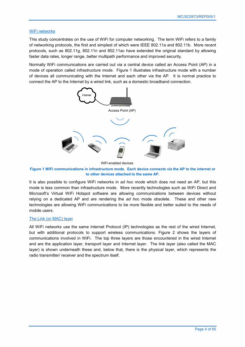
Normally WiFi communications are carried out via a central device called an Access Point (AP) in a
mode of operation called infrastructure mode. Figure 1 illustrates infrastructure mode with a number
of devices all communicating with the Internet and each other via the AP. It is normal practice to
connect the AP to the Internet by a wired link, such as a domestic broadband connection.
Access Point (AP)
WiFi-enabled devices Figure 1 WiFi communications in infrastructure mode. Each device connects via the AP to the internet or
to other devices attached to the same AP.
It is also possible to configure WiFi networks in ad hoc mode which does not need an AP, but this
mode is less common than infrastructure mode. More recently technologies such as WiFi Direct and
Microsoft’s Virtual WiFi Hotspot software are allowing communications between devices without
relying on a dedicated AP and are rendering the ad hoc mode obsolete. These and other new
technologies are allowing WiFi communications to be more flexible and better suited to the needs of
mobile users.
The Link (or MAC) layer
All WiFi networks use the same Internet Protocol (IP) technologies as the rest of the wired Internet,
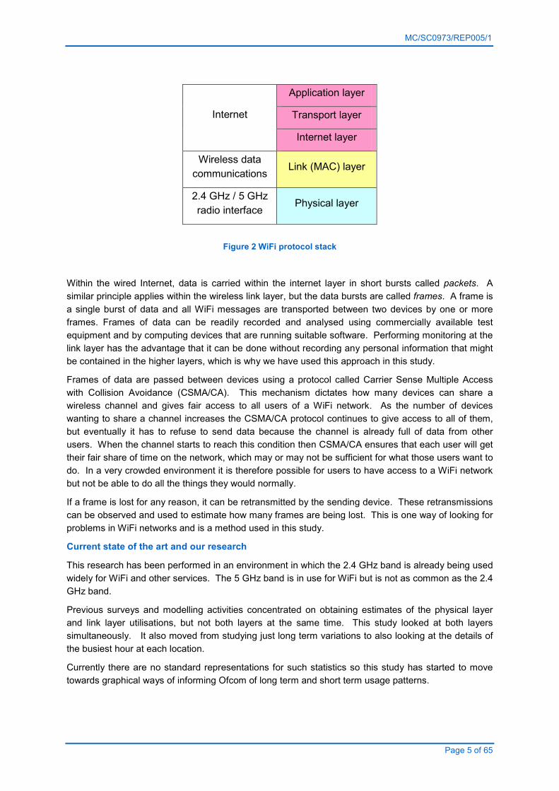
but with additional protocols to support wireless communications. Figure 2 shows the layers of
communications involved in WiFi. The top three layers are those encountered in the wired Internet
and are the application layer, transport layer and Internet layer. The link layer (also called the MAC
layer) is shown underneath these and, below that, there is the physical layer, which represents the
radio transmitter/ receiver and the spectrum itself.
MC/SC0973/REP005/1
Page 5 of 65
Application layer
Transport layer
Internet
Internet layer
Wireless data
communications Link (MAC) layer
2.4 GHz / 5 GHz
radio interface Physical layer
Figure 2 WiFi protocol stack
Within the wired Internet, data is carried within the internet layer in short bursts called packets. A
similar principle applies within the wireless link layer, but the data bursts are called frames. A frame is
a single burst of data and all WiFi messages are transported between two devices by one or more
frames. Frames of data can be readily recorded and analysed using commercially available test
equipment and by computing devices that are running suitable software. Performing monitoring at the
link layer has the advantage that it can be done without recording any personal information that might
be contained in the higher layers, which is why we have used this approach in this study.
Frames of data are passed between devices using a protocol called Carrier Sense Multiple Access
with Collision Avoidance (CSMA/CA). This mechanism dictates how many devices can share a
wireless channel and gives fair access to all users of a WiFi network. As the number of devices
wanting to share a channel increases the CSMA/CA protocol continues to give access to all of them,
but eventually it has to refuse to send data because the channel is already full of data from other
users. When the channel starts to reach this condition then CSMA/CA ensures that each user will get
their fair share of time on the network, which may or may not be sufficient for what those users want to
do. In a very crowded environment it is therefore possible for users to have access to a WiFi network
but not be able to do all the things they would normally.
If a frame is lost for any reason, it can be retransmitted by the sending device. These retransmissions
can be observed and used to estimate how many frames are being lost. This is one way of looking for
problems in WiFi networks and is a method used in this study.
Current state of the art and our research
This research has been performed in an environment in which the 2.4 GHz band is already being used
widely for WiFi and other services. The 5 GHz band is in use for WiFi but is not as common as the 2.4
GHz band.
Previous surveys and modelling activities concentrated on obtaining estimates of the physical layer
and link layer utilisations, but not both layers at the same time. This study looked at both layers
simultaneously. It also moved from studying just long term variations to also looking at the details of
the busiest hour at each location.
Currently there are no standard representations for such statistics so this study has started to move
towards graphical ways of informing Ofcom of long term and short term usage patterns.

MC/SC0973/REP005/1
Page 6 of 65
Conclusions
The study has concentrated on measuring ‘occupancy’ in the physical layer and ‘MAC stress’ as the
primary parameters for observing the state of these spectrum bands. It has also given results for the
‘network density’ and ‘throughput’, which are regarded as secondary parameters. With these four
parameters it is possible to form an understanding of the state of the LE bands used for WiFi
networking.
Figure 3 shows a high level view of the types of sites surveyed in terms of the primary parameters.
More site surveys would be needed to build up probability distributions of these parameters, so this
figure is an approximation based on our measurements.
Figure 3 Summaries of 2.4 GHz and 5 GHz environments showing the relatively higher physical layer
occupancy and MAC stress observed in cafés and shopping centres compared to houses and
apartments. The difference between sites was less pronounced in the 5 GHz band which exhibited
considerably lower occupancy and MAC stress.
Overall physical layer occupancy in the 2.4 GHz band was rated as moderate by the scale we have
used and it is rated as low in the 5 GHz band. High levels of occupancy were rare, suggesting that,
despite the large numbers of users of these bands (the 2.4 GHz band particularly), the bands are not
approaching their maximum capacity to carry WLAN traffic. We also did not see long periods of
sustained WiFi throughput compared to the maximum throughputs these bands are capable of
supporting.
Figure 4 summarises the network density and interference sources in the 2.4 GHz band, which is a
complex situation to explain graphically.

MC/SC0973/REP005/1
Page 7 of 65
The WiFi networks were exhibiting the signs of degraded performance, but this was mainly in the
shopping centre locations in the 2.4 GHz band where the median number of APs was over 60,
compared to below 10 for the other sites.
Whilst non-WiFi interference was observed to have a part to play in causing this degradation, there is
evidence in our results to strongly suggest that more of the problems can be attributed to the
overlapping channels in the 2.4 GHz band and the prevalence of tethered phones/ mobile hotspots in
public areas. In reading this result it must be remembered that there are many other factors affecting
WiFi network performance in addition to the radio spectrum constraints.
High network density in
shopping centres may be due to tethering
High MAC stress mainly
caused by WiFi channel overlap
Each icon represent the
busiest hour at a single location.
Interference to WiFi has
been assessed from all the busiest hour data
available in each grid square. The source of
the interference has been apportioned to either
‘WiFi’ or ‘Other’.
‘WiFi’ interference in the
2.4 GHz band is mainly attributable to the use of
overlapping channels.
‘Other’ interference can come from a wide variety
of other sources including Bluetooth, microwave
ovens, video senders and baby monitors.
‘Occupancy’ is a measure of how much spectrum is
used in both time and frequency. At high
occupancy it is likely that WiFi congestion will occur.
‘MAC Stress’ is a measure of whether the WiFi
networks are currently experiencing problems
carrying data or not.
Network density is a measure of how many
WiFi Access Points can be seen at each site.
Figure 4 MAC stress versus spectrum occupancy in the 2.4 GHz band with each icon representing the
busy hour from one survey. Icon colours show how many APs were seen at each site and the dial gauges
indicate the apportioning of interference to WiFi channel overlap or other source.
With very low utilisation of the 5 GHz band, where overlapping channels are not allowed, it would be
wise for users to migrate to this band. For those users whose hardware only supports 2.4 GHz
operations then we support the recommendation of others to use only channels 1, 6 and 11 to
minimise the probability of interference between networks.
As a measurement method, the relatively low cost dongles used in this study performed well. It is
possible to estimate the performance of WiFi networks using such equipment, but there are limits to
this. In particular, we were constrained to not intercept any user data, which severely limited our
ability to make inferences about the performance that users are likely to expect. Also having to scan
each channel sequentially meant that only a small amount of data was available for each one, limiting
the statistics that could be compiled at the granularity of channels. For whole band monitoring,
however, this constraint was not a problem.
The study revealed that long term monitoring to reveal diurnal activity patterns and short term
monitoring to understand peak demand in the busiest hour are both of interest to help inform Ofcom’s
policy decision making. We are recommending that future measurements be made at a time
resolution of 15 minutes for long term monitoring and 5 seconds for busiest hour monitoring.
MC/SC0973/REP005/1
Page 8 of 65
Document Authorisation
Prepared by: _______________________________________________________________
A.J. Wagstaff S. Day A. MacDonald
Principal Consultant Technical Consultant Principal Consultant
MASS Phasor Design MASS
Approved by: ________________________________________
J. Burr
Project Manager
Authorised by: ________________________________________
M. Ashman
Head of Systems Development
Change History
Version Date Change Details
1 19/6/13 First formal issue
Copyright © 2013 Mass Consultants Limited. All Rights Reserved.
The copyright and intellectual property rights in this work are vested in Mass Consultants Limited. This document
is issued in confidence for the sole purpose for which it is supplied and may not be reproduced, in whole or in part,
or used for any other purpose, except with the express written consent of Mass Consultants Limited.

MC/SC0973/REP005/1
Page 9 of 65
Contents
1 Introduction 10
2 Background 11
2.1 MASS studies 11
2.2 Other studies 12
3 Research questions and drivers 18
3.1 Formal research questions 18
3.2 Questions arising during study 19
3.3 Other drivers for the research 19
4 Research method 21
4.1 Monitoring system 21
4.2 Approaches to representation and interpretation 21
4.3 Primary and secondary measurement parameters 25
4.4 Laboratory tests 30
4.5 Field surveys 32
5 Results 33
5.1 Occupancy 34
5.2 MAC stress 37
5.3 Occupancy and MAC stress 40
5.4 Throughput 41
5.5 Network density 44
5.6 Interference from services other than WiFi 47
5.7 Mutual degradation between WiFi networks 48
5.8 Fine time resolution 51
6 Conclusions and further work 55
6.1 Occupancy 55
6.2 MAC stress 55
6.3 Occupancy and MAC stress 56
6.4 Network density 56
6.5 WiFi throughput 56
6.6 Practicality of the measurement method 57
6.7 Further work 57
7 Glossary of Terms 59
8 Definitions 60
9 References 61
10 Bibliography 65

MC/SC0973/REP005/1
Page 10 of 65
1 INTRODUCTION
This is the final report on the project entitled ‘Utilisation of key Licence Exempt bands and the effects
on WLAN performance’ which has been undertaken for Ofcom by MASS.
The project aimed to measure the physical and link layer usage of the 2.4 GHz and 5 GHz Licence
Exempt bands with particular emphasis on the use of these bands for Wireless Local Area Networks
(WLAN) by the IEEE 802.11 ‘WiFi’ family of protocols. It developed a measurement method that uses
relatively low-cost dongles with a view to becoming a standard technique that can be used by Ofcom
for future surveys.
Section 2 looks at the background research results available. Section 3 then details the research
questions that this study aimed to answer. Section 4 describes the measurement method and section
5 gives the results (with further detail in the Appendices). The conclusions and further work are in
section 6.
MC/SC0973/REP005/1
Page 11 of 65
2 BACKGROUND
This section looks at previous, relevant studies that have been carried out by MASS and other
organisations.
There is increasing pressure to use the 2.4 GHz and 5 GHz bands for WiFi-based applications at the
same time as their use for other applications such as wireless sensor networking. Particularly notable
is the move towards cellular offloading onto WiFi (Lee et al, 2010) (Dimmateo et al, 2011) which could
affect these LE bands if not supported via alternative spectrum allocations.
2.1 MASS studies
MASS can draw upon several years of actively working with Ofcom to measure utilisation, interference
and congestion in the Licence Exempt (LE) bands. Our work in this area started in 2002 with physical
layer measurements in the 2.4 GHz band for the Radiocommunications Agency. The first study
looked at band utilisation plus daily and weekly variations (Day and Merricks, 2003) and found that
levels of activity were generally low. Microwave ovens and movement detectors were observed and
where 802.11 traffic was seen there was not much use of the physical layer.
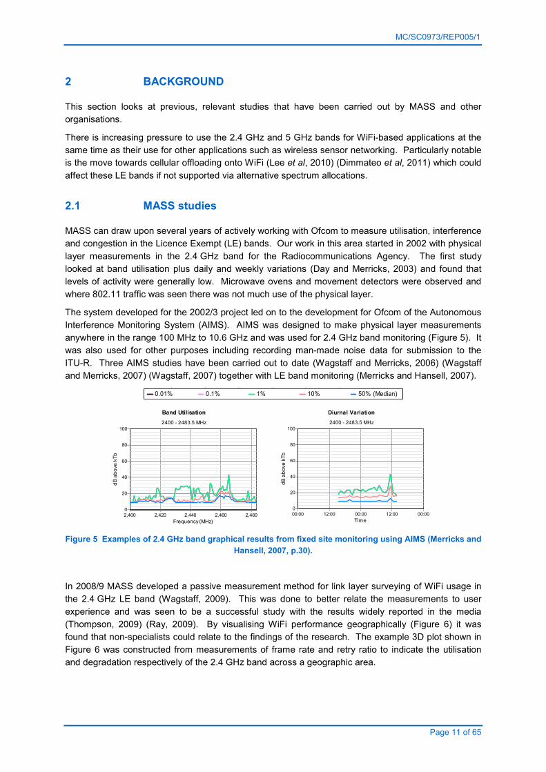
The system developed for the 2002/3 project led on to the development for Ofcom of the Autonomous
Interference Monitoring System (AIMS). AIMS was designed to make physical layer measurements
anywhere in the range 100 MHz to 10.6 GHz and was used for 2.4 GHz band monitoring (Figure 5). It
was also used for other purposes including recording man-made noise data for submission to the
ITU-R. Three AIMS studies have been carried out to date (Wagstaff and Merricks, 2006) (Wagstaff
and Merricks, 2007) (Wagstaff, 2007) together with LE band monitoring (Merricks and Hansell, 2007).
0.01% 0.1% 1% 10% 50% (Median)
Band Utilisation
2400 - 2483.5 MHz
Frequency (MHz)
2,4802,4602,4402,4202,400
dB above kTb
100
80
60
40
20
0
Diurnal Variation
2400 - 2483.5 MHz
Time
00:0012:0000:0012:0000:00
dB above kTb
100
80
60
40
20
0
Figure 5 Examples of 2.4 GHz band graphical results from fixed site monitoring using AIMS (Merricks and
Hansell, 2007, p.30).
In 2008/9 MASS developed a passive measurement method for link layer surveying of WiFi usage in
the 2.4 GHz LE band (Wagstaff, 2009). This was done to better relate the measurements to user
experience and was seen to be a successful study with the results widely reported in the media
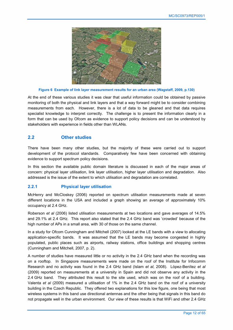
(Thompson, 2009) (Ray, 2009). By visualising WiFi performance geographically (Figure 6) it was
found that non-specialists could relate to the findings of the research. The example 3D plot shown in
Figure 6 was constructed from measurements of frame rate and retry ratio to indicate the utilisation
and degradation respectively of the 2.4 GHz band across a geographic area.
MC/SC0973/REP005/1
Page 12 of 65
Figure 6 Example of link layer measurement results for an urban area (Wagstaff, 2009, p.130)
At the end of these various studies it was clear that useful information could be obtained by passive
monitoring of both the physical and link layers and that a way forward might be to consider combining
measurements from each. However, there is a lot of data to be gleaned and that data requires
specialist knowledge to interpret correctly. The challenge is to present the information clearly in a
form that can be used by Ofcom as evidence to support policy decisions and can be understood by
stakeholders with experience in fields other than WLANs.
2.2 Other studies
There have been many other studies, but the majority of these were carried out to support
development of the protocol standards. Comparatively few have been concerned with obtaining
evidence to support spectrum policy decisions.
In this section the available public domain literature is discussed in each of the major areas of
concern: physical layer utilisation, link layer utilisation, higher layer utilisation and degradation. Also
addressed is the issue of the extent to which utilisation and degradation are correlated.
2.2.1 Physical layer utilisation
McHenry and McCloskey (2006) reported on spectrum utilisation measurements made at seven
different locations in the USA and included a graph showing an average of approximately 10%
occupancy at 2.4 GHz.
Roberson et al (2006) listed utilisation measurements at two locations and gave averages of 14.5%
and 29.1% at 2.4 GHz. This report also stated that the 2.4 GHz band was ‘crowded’ because of the
high number of APs in a small area, with 30 of those on the same channel.
In a study for Ofcom Cunningham and Mitchell (2007) looked at the LE bands with a view to allocating
application-specific bands. It was assumed that the LE bands may become congested in highly
populated, public places such as airports, railway stations, office buildings and shopping centres
(Cunningham and Mitchell, 2007, p. 2).
A number of studies have measured little or no activity in the 2.4 GHz band when the recording was
on a rooftop. In Singapore measurements were made on the roof of the Institute for Infocomm
Research and no activity was found in the 2.4 GHz band (Islam et al, 2008). López-Benítez et al
(2009) reported on measurements at a university in Spain and did not observe any activity in the
2.4 GHz band. They attributed this result to the site used, which was on the roof of a building.
Valenta et al (2009) measured a utilisation of 1% in the 2.4 GHz band on the roof of a university
building in the Czech Republic. They offered two explanations for this low figure, one being that most
wireless systems in this band use directional antennas and the other being that signals in this band do
not propagate well in the urban environment. Our view of these results is that WiFi and other 2.4 GHz

MC/SC0973/REP005/1
Page 13 of 65
technologies tend to be used predominantly at ground level and the relatively low levels of transmitted
power are attenuated heavily before reaching the rooftops.
These utilisation results can be compared with those from the MASS studies. We found that the
average utilisation was 5.7% in 2003 and it rose to 14.3% in 2006 (Wagstaff, 2009, p. 35). These
results were based on three sites at which it had been possible to repeat the measurement method.
The difficulties with the logistics of repeating measurements have to be borne in mind when
interpreting any statistics of spectrum utilisation.
2.2.2 Link layer utilisation
Bianchi (1998) modelled the link layer utilisation for a number of clients accessing a single Access
Point (AP) and no interference from other WiFi networks or non-WiFi transmitters. The results
indicated a saturated throughput (i.e. the maximum total data rate in the link layer) of between 55%
and 85% depending on network configuration parameters.
Jardosh et al (2005a) observed congestion when the observed total MAC layer throughput
approached the maximum possible 5.5Mbps on a network of 38 IEEE 802.11b APs at a conference in
2005.
Duda (2008) analysed the access mechanism used in the MAC layer and showed how the available
throughput suffers from short-term unfairness when there is a large number of clients.
Raghavendra et al (2009) analysed a series of link layer measurements of utilisation in apartment
blocks, single family houses, enterprise networks, a large conference centre and at a coffee shop
hotspot. Their analysis suggested a median link layer utilisation of between 30% and 40% and they
attributed these relatively low levels to low demand rather than interference from other networks or
other factors.
2.2.3 Higher layer utilisation
Simek et al (2011, p.293) made 2.4 GHz band measurements in a block of flats in the Czech Republic
and observed that 802.11g was the predominant standard at that time. 802.11b was used 5.9% of the
time, 802.11g was used 71.3% and 802.11n was used 22.8%.
Gember et al (2011) observed that the type of content being used depends on the type of client
device. For non-handheld devices only 17% of the content is video but this rises to 40% for handheld
devices.
Sen et al (2011) reported an important result for this study. In their work they measured the Allan
deviation (Allan, 1987) of higher layer network traffic at different locations and found that the
aggregation period giving minimum Allan deviation varied considerably by location. In their examples
it was found to be 15 minutes at one location and 75 minutes at another. The implication of this is that
a measurement method either has to specify fixed aggregation periods and accept estimation
variability or it can use an adaptive approach where the aggregation period is optimised to give
minimum variability.
Sommers and Barford (2012) reported on the results of SpeedTest measurements on a variety of WiFi
networks. The SpeedTest software performs tests using HTTP so these results are indicative of the
higher layer utilisation. They found that WiFi performance generally exceeded cellular performance
and that the performance varied greatly with location and time of day. Detailed statistics were not
given in the paper but the peak user traffic was less than 20Mbps and the median was clearly less
than 10Mbps.
Recent approaches to modelling network traffic have been based on wavelet concepts that allow
multiscale effects and long range dependency to be simulated in higher layer WiFi traffic models (Tian
et al, 2002)(Fei and Yu, 2008)(Han-Lin et al, 2009). In these approaches packet arrival times are
MC/SC0973/REP005/1
Page 14 of 65
assumed to be independent at small timescales, but long range dependency emerges as longer
timescales are considered.
2.2.4 Degradation
The reliability of WiFi networking is a recurring theme with many factors affecting the reliability
perceived by users. Wong and Clement (2006) stated that the many respondents to their
questionnaire on sharing WiFi were concerned about reliability. Similarly Sheth et al (2006) reported
that that the unreliable nature of WiFi links meant that users frequently experienced degraded
performance and lack of coverage in enterprises and university campuses.
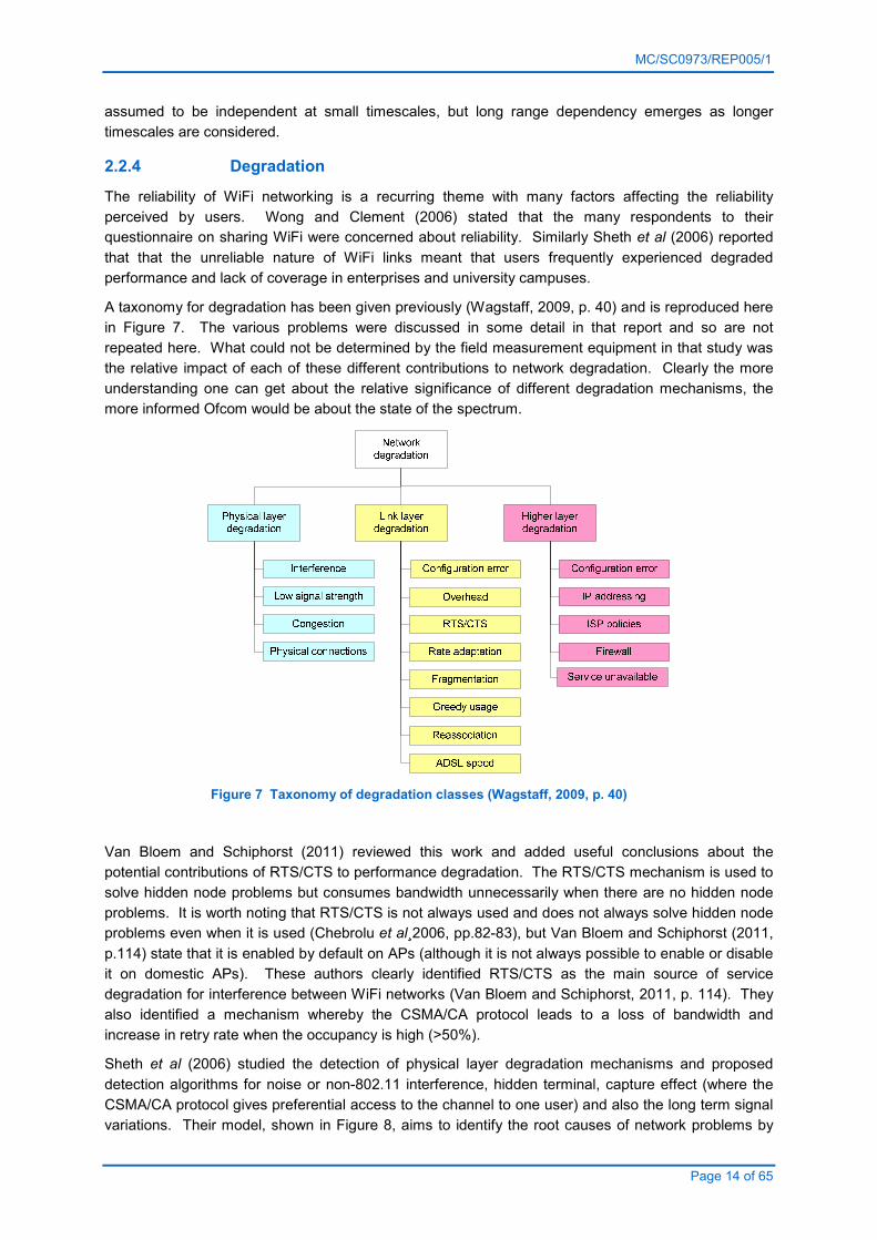
A taxonomy for degradation has been given previously (Wagstaff, 2009, p. 40) and is reproduced here
in Figure 7. The various problems were discussed in some detail in that report and so are not
repeated here. What could not be determined by the field measurement equipment in that study was
the relative impact of each of these different contributions to network degradation. Clearly the more
understanding one can get about the relative significance of different degradation mechanisms, the
more informed Ofcom would be about the state of the spectrum.
Figure 7 Taxonomy of degradation classes (Wagstaff, 2009, p. 40)
Van Bloem and Schiphorst (2011) reviewed this work and added useful conclusions about the
potential contributions of RTS/CTS to performance degradation. The RTS/CTS mechanism is used to
solve hidden node problems but consumes bandwidth unnecessarily when there are no hidden node
problems. It is worth noting that RTS/CTS is not always used and does not always solve hidden node
problems even when it is used (Chebrolu et al¸2006, pp.82-83), but Van Bloem and Schiphorst (2011,
p.114) state that it is enabled by default on APs (although it is not always possible to enable or disable
it on domestic APs). These authors clearly identified RTS/CTS as the main source of service
degradation for interference between WiFi networks (Van Bloem and Schiphorst, 2011, p. 114). They
also identified a mechanism whereby the CSMA/CA protocol leads to a loss of bandwidth and
increase in retry rate when the occupancy is high (>50%).
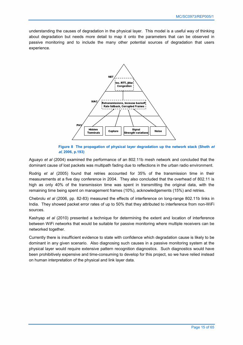
Sheth et al (2006) studied the detection of physical layer degradation mechanisms and proposed
detection algorithms for noise or non-802.11 interference, hidden terminal, capture effect (where the
CSMA/CA protocol gives preferential access to the channel to one user) and also the long term signal
variations. Their model, shown in Figure 8, aims to identify the root causes of network problems by
MC/SC0973/REP005/1
Page 15 of 65
understanding the causes of degradation in the physical layer. This model is a useful way of thinking
about degradation but needs more detail to map it onto the parameters that can be observed in
passive monitoring and to include the many other potential sources of degradation that users
experience.
Figure 8 The propagation of physical layer degradation up the network stack (Sheth et
al, 2006, p.193)
Aguayo et al (2004) examined the performance of an 802.11b mesh network and concluded that the
dominant cause of lost packets was multipath fading due to reflections in the urban radio environment.
Rodrig et al (2005) found that retries accounted for 35% of the transmission time in their
measurements at a five day conference in 2004. They also concluded that the overhead of 802.11 is
high as only 40% of the transmission time was spent in transmitting the original data, with the
remaining time being spent on management frames (10%), acknowledgements (15%) and retries.
Chebrolu et al (2006, pp. 82-83) measured the effects of interference on long-range 802.11b links in
India. They showed packet error rates of up to 50% that they attributed to interference from non-WiFi
sources.
Kashyap et al (2010) presented a technique for determining the extent and location of interference
between WiFi networks that would be suitable for passive monitoring where multiple receivers can be
networked together.
Currently there is insufficient evidence to state with confidence which degradation cause is likely to be
dominant in any given scenario. Also diagnosing such causes in a passive monitoring system at the
physical layer would require extensive pattern recognition diagnostics. Such diagnostics would have
been prohibitively expensive and time-consuming to develop for this project, so we have relied instead
on human interpretation of the physical and link layer data.
MC/SC0973/REP005/1
Page 16 of 65
2.2.5 Correlation between degradation and utilisation
Currently there is very little evidence for correlation between the degradation and utilisation of a WLAN
(Raghavendra, et al, 2009, p.4), (Wagstaff, 2009, p.18).
Early work in the area was the development of the N-systems method, which led to conclusions on the
number of APs that could share a channel in an area. This study identified numbers in the order of 24
APs in a 1km2 area (Hansel et al, 2004, p.vi) but the polite protocols used by 802.11 and burstiness of
traffic mean that, in practice, much higher densities can be expected to be supportable in the LE
bands.
In 2006 a report by Scientific Generics asserted that interference between WLANs in the 2.4 GHz
band existed, but only in areas of high usage (Scientific Generics, 2006, p. 8) and, on that basis,
recommended increasing the power levels allowed in rural areas.
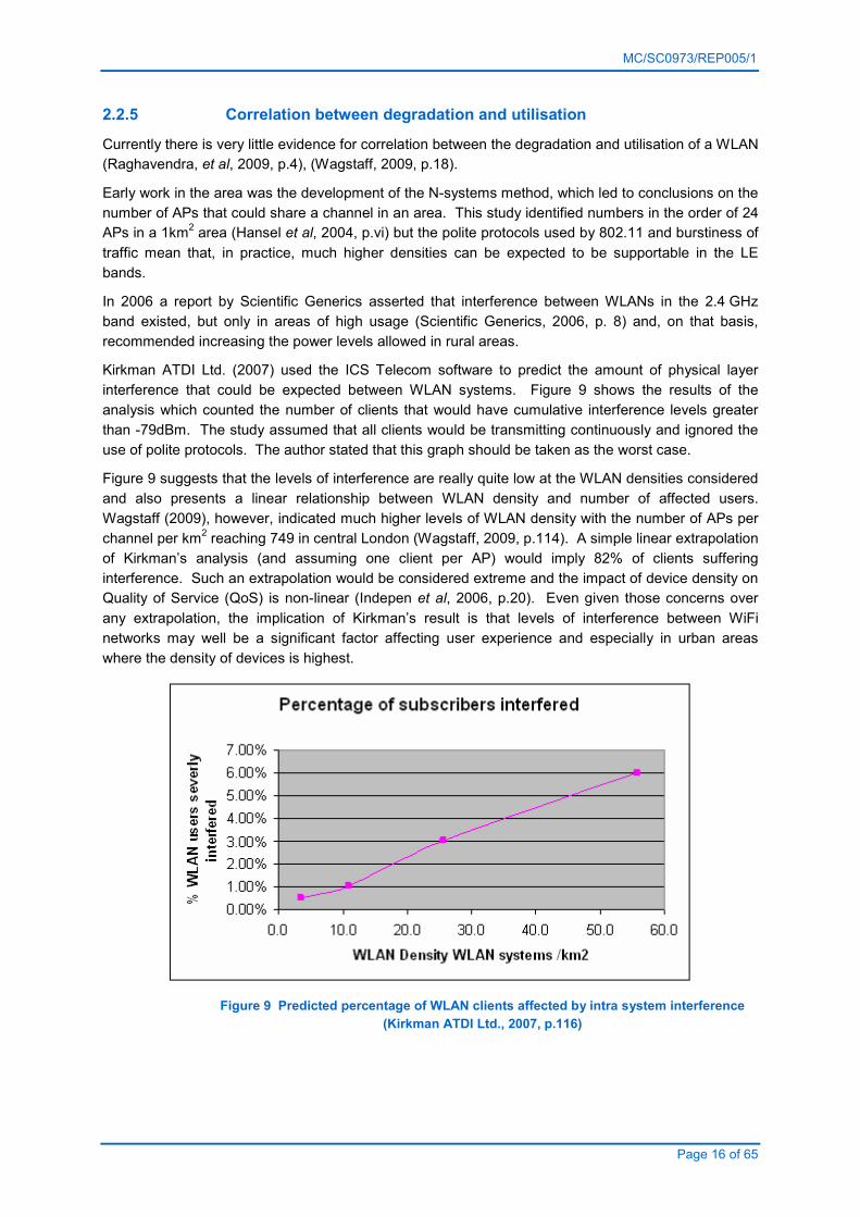
Kirkman ATDI Ltd. (2007) used the ICS Telecom software to predict the amount of physical layer
interference that could be expected between WLAN systems. Figure 9 shows the results of the
analysis which counted the number of clients that would have cumulative interference levels greater
than -79dBm. The study assumed that all clients would be transmitting continuously and ignored the
use of polite protocols. The author stated that this graph should be taken as the worst case.
Figure 9 suggests that the levels of interference are really quite low at the WLAN densities considered
and also presents a linear relationship between WLAN density and number of affected users.
Wagstaff (2009), however, indicated much higher levels of WLAN density with the number of APs per
channel per km2 reaching 749 in central London (Wagstaff, 2009, p.114). A simple linear extrapolation
of Kirkman’s analysis (and assuming one client per AP) would imply 82% of clients suffering
interference. Such an extrapolation would be considered extreme and the impact of device density on
Quality of Service (QoS) is non-linear (Indepen et al, 2006, p.20). Even given those concerns over
any extrapolation, the implication of Kirkman’s result is that levels of interference between WiFi
networks may well be a significant factor affecting user experience and especially in urban areas
where the density of devices is highest.
Figure 9 Predicted percentage of WLAN clients affected by intra system interference
(Kirkman ATDI Ltd., 2007, p.116)

MC/SC0973/REP005/1
Page 17 of 65
Cisco (2004) performed tests on different channel 802.11b and 802.11g AP configurations. They
recommended that three non-overlapping channel arrangements were much better than four channel
configurations where the channels overlapped slightly.
Metageek (2012) state that it is best to choose AP channels that are not overlapping, but if that is not
possible then it is better to share channels than to use adjacent, overlapping channels. For sharing of
channels to work effectively then they recommend looking for 20dB separation between APs that are
on the same channel. This advice (and variations thereof) is repeated many times on the internet (e.g.
Horowitz, 2012).
Coleman (2012) advised against the four channel scheme (channels 1, 5, 9 and 13) that can be used
in Europe. There is some frequency overlap with this scheme and he suggested that it would be
better to use co-channel operation (i.e. 1, 6 and 11) where the medium contention can work
effectively. He emphasised that 1, 6 and 11 are likely to be used by neighbouring networks, so
adopting 1, 5, 9 and 13 is likely to interfere with and suffer interference from those networks.
There is currently little hard evidence to produce reliable conclusions on the relationships between the
utilisation of WiFi and levels of interference and other degradation to be expected, especially in dense
urban areas. There would be a lot to be gained by combining modelling with field measurements, as
currently the assumptions in the models are too simplistic and the field measurements cannot be
easily interpolated or extrapolated to other locations. Our recommendation is that Ofcom considers a
combined study with detailed field measurements being used to calibrate a model at different
densities. This work is outside the scope of the current measurement study.

MC/SC0973/REP005/1
Page 18 of 65
3 RESEARCH QUESTIONS AND DRIVERS
The work carried out during this project has been aimed at answering the original, formal research
questions, but has also been influenced by questions from Ofcom that have arisen. It has further been
influenced by specific market drivers that are affecting the development of WLAN technology and
usage.
3.1 Formal research questions
The original research questions were given in the Invitation to Tender (ITT) document (Ofcom, 2012)
and reiterated in MASS’s proposal (Wagstaff, 2012).
1. Is it possible to devise a robust, repeatable approach to measuring utilisation of the 2.4 GHz
and 5 GHz LE bands and link this to the quality of service experienced by users?
2. Are Wi-Fi devices currently experiencing a degradation of service, e.g. congestion, interference,
incorrect configuration of devices? Where and when is degradation occurring? What steps could
be taken to mitigate these problems?
These questions were partly addressed in the 2008/9 study (Wagstaff, 2009, p.16) where the research
question was:
• Is it possible to define one or more technical measures of network congestion that can be
obtained by passive monitoring and can be easily related to user experience of network
congestion?
Further discussions with Ofcom at the start of the project refined the concerns and constraints. The
following points emerged that helped to clarify the measurements that are needed:
• As with all other Ofcom projects concerns over data protection meant that it was not possible to
examine any of the user data. To address this concern the capture software was written such
that it rejected all MAC data apart from the frame headers. No data from the IP or application
layers was captured. It is important to note that this constrained approach to data capture is
markedly different from the majority of studies by other researchers that capture all data
regardless of content;
• Earlier projects have looked at either the PHY or the MAC layer and, separately, produced
useful information. Moving to a system that captured and analysed both was expected to
produce information that would be even more useful to Ofcom. The hardware for such a system
could have been prohibitively expensive, so the decision was taken to experiment with relatively
low cost dongles to see if these could produce data with sufficient fidelity to inform the regulator
with confidence about the state of the spectrum;
• In the 2008/9 study the emphasis was on a geographic view of different locations. In the current
study the emphasis changed to be on specific types of location. In particular Ofcom were
interested in housing blocks (flats or apartments) and the wireless hot spot areas in and around
cafés or coffee shops. This was extended during the study to include shopping centres as a
category;
• The spectrum can be observed either by passively listening or by actively stimulating it by
transmitting a signal and observing the characteristics of the received signal. Ofcom prefer
passive sensing;

MC/SC0973/REP005/1
Page 19 of 65
• Ofcom are particularly interested in understanding the radio environment in these bands in
terms of spectrum occupancy, numbers of Access Points (AP) and retry rate. The first of these
is a physical layer quantity, the latter two are observed in the link layer.
3.2 Questions arising during study
During the development of the measurement method the following questions arose that significantly
affected the course of the study:
1. What parameters should be recorded and how should data be visualised in order to convey the
information required?
A great many parameters could be recorded, analysed and reported on, in fact there
are so many that it is easy to get confused by all the data. It became clear that
current data visualisation approaches are lacking when it comes to showing what is
happening.
2. Over what period should data be aggregated?
With so much data readily available it is necessary to agree on a data reduction
scheme. Any data reduction approach involves some degree of aggregation and
there is a risk that this will either be too much or too little for the required application.
Ofcom stated that they would want to be able to run a monitoring system continuously
for one or two weeks to be able to understand usage variability over a reasonable
long period. It is unlikely that monitoring will be carried out over periods of months or
longer.
Earlier work on similar monitoring systems designed by MASS suggested that
reporting at one hour intervals would be suitable. It is now noted that Sen et al (2011)
identified considerable differences in the best reporting intervals for higher layer data
at different locations and this observation is likely to affect the design of future
monitoring systems.
As the project proceeded it became clear that attention was being drawn naturally to
the busiest hour of a day. This implied an aggregation period of less than one hour so
that the statistics of the busiest hour could be investigated.
The study was extended to look at a shorter aggregation interval. In the rest of the
report we use the term ‘coarse time resolution’ to indicate the one hour averaging
used in the first part of the study and ‘fine time resolution’ to refer to the 5 and 330
second averaging intervals that were added to the monitoring method for the second
part of the study.
3.3 Other drivers for the research
The globally increasing use of wireless internet access is without doubt the main driver for
understanding the state of the LE bands in which WiFi can be used. There are a number of market
drivers that derive from this that have affected the thinking behind the research method.
1. Offloading cellular capacity to WiFi is a move that would help the cellular operators meet
demand for mobile internet access (Lee et al, 2010)(Dimmateo, 2011);

MC/SC0973/REP005/1
Page 20 of 65
2. It is predicted that consumer demand for non-linear services will mean that all future TV
receivers will have internet connectivity (EBU, 2011). Smart TVs are already available in UK
stores that include built-in WiFi or have WiFi dongles (e.g. LG AN-WF100, Toshiba WLM-20U2)
to give internet access. These will be used for streaming video from a wide variety of sources
(e.g. BBC iPlayer, 4oD, Netflix, YouTube, Vimeo);
3. Demand for additional 5 GHz spectrum to support future wireless internet access has been
highlighted recently (Williamson et al, 2013). This demand is based on modelling of a number
of use cases that show demand outstripping spectrum capacity well before 2020;
4. There are ongoing developments to the IEEE 802.11 standards within the existing 2.4 GHz and
5 GHz bands. IEEE 802.11aa covers improvements to the transport of video (Maraslis et al,
2012). IEEE 802.11ac will enable bandwidths up to 160 MHz to be used in the 5 GHz band;
5. There are a number of developments relating to data networking that will require spectrum in
bands other than those considered by this research. Specific examples include the ‘TV white
space’ technologies such as IEEE 802.11af (“White-Fi”), IEEE 802.22 (broadband access in
white space) and the Weightless protocol (M2M in white space). The IEEE 802.11ah protocol is
being aimed at other frequency bands below 1 GHz for sensor networking. Also there are
moves to make more use of the 60 GHz band for high speed data transfers involving
technologies such as IEEE 802.11ad (“WiGig”). All these developments are seen as
alternative, free to the end customer, technologies that will be able to deliver services currently
delivered by the 2.4 GHz and 5 GHz bands. They may serve to relieve the pressure of demand
on these bands and thereby slow the seemingly inexorable rise in spectrum occupancy;
6. Looking further afield there are other technology developments that could alleviate congestion
issues in the 2.4 GHz and 5 GHz bands. To allow different protocols to share bands more
effectively one line of enquiry is the Gap Sense technology being investigated at the University
of Michigan (Zhang and Shin, 2013). Various multiuser MIMO schemes have been proposed to
share spectrum more effectively. One such example is Vandermonde frequency division
multiplexing which has been proposed for cognitive radio applications and could be applied to
systems operating in the 2.4 GHz and 5 GHz bands (Cardoso et al, 2008).

MC/SC0973/REP005/1
Page 21 of 65
4 RESEARCH METHOD
This section describes the monitoring system, the laboratory tests and field surveys.
4.1 Monitoring system
Three identical monitoring systems were assembled for this project. The emphasis was on relatively
low cost hardware that could monitor both the PHY and MAC layers and could be easily deployed.
It was found that the two primary and two secondary parameters (see Section 4.3) could be monitored
over at least a day and that it was relatively straightforward to set the equipment up in the field.
The monitoring systems were run in the laboratory prior to carrying out the field surveys. These tests
confirmed that the system gave the same results when running in the same environment, that all the
data required was being captured correctly and that the graphical outputs used in this report were
calibrated correctly.
Details of the monitoring system are given in Appendix 3 together with recommendations for the
requirements to be placed on the design of future monitoring systems.
4.2 Approaches to representation and interpretation
The data collected during the field surveys is complex and difficult to interpret at a high level. It is
possible to see differences between 2.4 GHz and 5 GHz band usage, diurnal variations with
pronounced busy hours and other effects in the data, but there is no standard way of presenting this
information.
Selecting the data representations emerged as a key issue because no single representation conveys
a clear view of what is happening. Sometimes the information gleaned can feel counterintuitive so the
data representation must be clear and unequivocal.
During this project a variety of data representation approaches have been proposed and investigated.
These include:
1. Low-level data visualisation – Low-level graphs have been produced for all the data (see
Appendix 1). These were the starting point for all the analysis, but require expert interpretation.
2. High-level data visualisation – A variety of high-level visualisations have been investigated.
These would require considerable further work in order to gain wide acceptance by the
community so have not been progressed further here.
3. Capacity model – This attempted to characterise the utilisation of the spectrum in terms of bit
rate, on the assumption that it is possible to define a maximum bit rate for a band and observe
how much of that capacity is being used at any given site. Such an approach was appealing in
that it could indicate how empty or full the current WiFi bands are. A significant weakness of it
was that it is not a simple matter to agree on the maximum data rate that can be supported,
because continual performance improvements in WiFi technology are delivering ever higher
data rates within the existing spectrum allocations. The capacity model was dropped in favour
of the throughput scale that is introduced in section 4.3.
4. Bayesian model – With the observation that different types of environment exhibit themselves
via multiple observable parameters (e.g. number of retries, number of RTS/CTS frames) with

MC/SC0973/REP005/1
Page 22 of 65
varying degrees of correlation between them, a Bayesian approach was proposed. This
method would recognise an environmental category by examining the probability distributions of
each parameter. The method is appealing technically but would require extensive laboratory
work to define the a priori distributions to a level of confidence that would be acceptable to
MASS. This would have been too time-consuming for this project. Universities are being
approached with a view to developing this model further.
5. Single parameter scales – This was the approach that was eventually adopted. Primary and
secondary parameters have been identified (see section 4.3) and these have been given
subjective scales to assist the reader with interpreting the results. It was felt that this method
would be pragmatic and acceptable to the greatest number of stakeholders.
These various approaches have led to a number of graphical data representations that have been
used to plot the LE band usage in time and frequency and also to summarise the usage by type of
location.
Low-level data visualisation
The usage of the LE bands in frequency has been analysed by inspecting summary frequency plots.
Figure 10 shows an example of the summary frequency plots that have been produced for each
survey. These show both MAC and PHY data and show how the LE bands are being used. The
upper set of three graphs show the parameters that can be shown on a power scale (dBm) and the
lower three graphs show averages of the measurements used to generate the primary and secondary
parameters.
2.4 GHz 5 GHz
Physical Layer
Link (MAC) Layer
Figure 10 Example of a set of summary frequency plots
MC/SC0973/REP005/1
Page 23 of 65
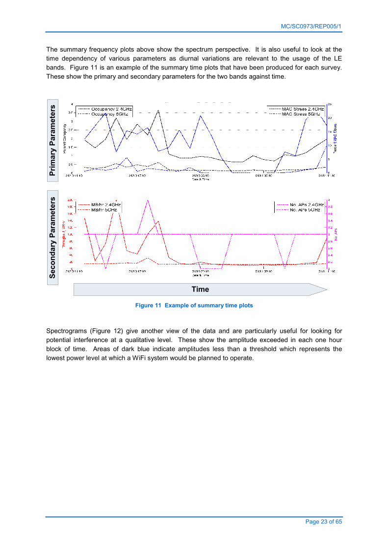
The summary frequency plots above show the spectrum perspective. It is also useful to look at the
time dependency of various parameters as diurnal variations are relevant to the usage of the LE
bands. Figure 11 is an example of the summary time plots that have been produced for each survey.
These show the primary and secondary parameters for the two bands against time.
Primary Parameters
Secondary Parameters
Time
Figure 11 Example of summary time plots
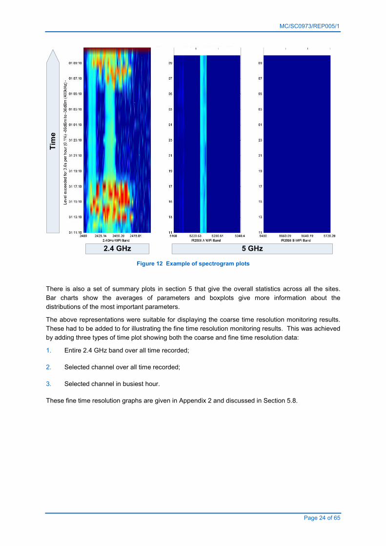
Spectrograms (Figure 12) give another view of the data and are particularly useful for looking for
potential interference at a qualitative level. These show the amplitude exceeded in each one hour
block of time. Areas of dark blue indicate amplitudes less than a threshold which represents the
lowest power level at which a WiFi system would be planned to operate.
MC/SC0973/REP005/1
Page 24 of 65
2.4 GHz 5 GHz
Tim
e
Figure 12 Example of spectrogram plots
There is also a set of summary plots in section 5 that give the overall statistics across all the sites.
Bar charts show the averages of parameters and boxplots give more information about the
distributions of the most important parameters.
The above representations were suitable for displaying the coarse time resolution monitoring results.
These had to be added to for illustrating the fine time resolution monitoring results. This was achieved
by adding three types of time plot showing both the coarse and fine time resolution data:
1. Entire 2.4 GHz band over all time recorded;
2. Selected channel over all time recorded;
3. Selected channel in busiest hour.
These fine time resolution graphs are given in Appendix 2 and discussed in Section 5.8.

MC/SC0973/REP005/1
Page 25 of 65
4.3 Primary and secondary measurement parameters
Much of the work has concentrated on finding representations of the data that can show what is
happening in the LE bands to answer the many questions that can and do arise. There are many
parameters that can be monitored. After considering many ways of looking at the data we have
decided to report mainly on two ‘primary’ parameters (physical layer occupancy and MAC stress) and
two ‘secondary’ parameters (network density and throughput). All other parameters are regarded here
as ‘tertiary’.
The term ‘primary’ is used here in the sense that these parameters are those of most interest to
Ofcom for the purposes of assessing the utilisation and degradation of the LE bands. The term
‘secondary’ is used for those parameters that inform the reader and help with understanding, but they
are less important than the primary parameters for understanding the state of the spectrum and,
indeed, can sometimes be misleading. The ‘tertiary’ parameters are only considered when it is
necessary to understand a particular phenomenon in some technical depth.
Primary parameter: Occupancy (physical layer utilisation)
The physical layer utilisation is used to show how much the LE bands are being used by all
services (WiFi, Bluetooth, ANT/ANT+, ZigBee, video senders, microwave ovens, etc.).
Alternative parameters (e.g. frame rate, bit rate, throughput) have been discarded in favour of
physical layer utilisation. For improved understanding this report abbreviates the term
physical layer utilisation to occupancy.
Occupancy is measured in the physical layer using the WiSpy DBx dongle and is the
percentage of time for which the received signal strength is above a threshold of -86 dBm in
400 kHz measurement bandwidth. This level corresponds to the lowest level that a WiFi
system might be planned to operate at, with adjustment for measurement bandwidth. It is
approximately 10dB above the noise floor of the monitoring equipment.
In order to give a subjective rating for the occupancy we have used the following scale in this
report.
Mean occupancy in
busiest hour
Occupancy category
Above 20% High
5% to 20% Moderate
Below 5% Low
Below 1% None
This is based on the interpretation of previous research results (see section 2.2.1). Merricks
and Hansell (2007) produced graphs of Relative Time & Frequency Utilisation (RTFU) at a
number of locations and it is these, together with the measurements made in the current study
and the older graphs in Day and Merricks (2003) that have most influenced the occupancy
scale above.
In further support of this scale the following table provides appropriate references. Occupancy
is called different things and measured in different ways so it is not a trivial matter to compare
these sources. The majority of the academic literature refers to single channel occupancy and

MC/SC0973/REP005/1
Page 26 of 65
tends to assume a relationship between spectral occupancy and WiFi degradation, so we
have had to apply some judgement to interpret these sources in terms of the occupancy of a
band.
Occupancy Comment Reference
> 80% Highly congested Jardosh et al (2005b)
> 50% Degradation due to CTS/RTS Van Bloem and Schiphorst (2011, p. 114)
30% - 84% Moderately congested Jardosh et al (2005b)
< 40% Underutilised Raghavendra et al (2009)
< 30% Uncongested Jardosh et al (2005b)
< 30% Quite low utilisation Raghavendra et al (2009)
9% Dearth of activity Merricks and Hansell (2007, p.30)
< 1% Unused López-Benítez et al (2009)
See sections 5.1 and 5.3 for discussion of the results of the occupancy monitoring.
Primary parameter: MAC stress (retry ratio)
MAC stress is the second of the two primary parameters and is used to show how much
degradation there is in the WiFi MAC layer.
It is measured in the MAC using the AirPcap Nx dongle and is the percentage of WiFi frames
that have the retry flag set. In our previous study we suggested a scale whereby the mean
retry ratio suggests a correlation with the user experience Wagstaff (2009, p. 75). In this study
we have concluded that the scale is a helpful one, but the correlation with user experience is
not clear. Instead we suggest that the retry ratio should be regarded as a ‘state of the MAC’
indicator only.
For the purposes of categorising the results in this report we have used the following colour
scale to indicate the level of ‘stress’ the MAC is under. The word ‘stress’ is used here to
convey the idea that the MAC is subject to varying levels of demand for traffic and varying
radio channel conditions experienced by the PHY. We have relaxed the categories from the
2009 definitions, recognising that a great many user applications do not need prolonged use
of the MAC and that it is not now thought possible to provide a single indication of user
experience from PHY and MAC measurements alone.
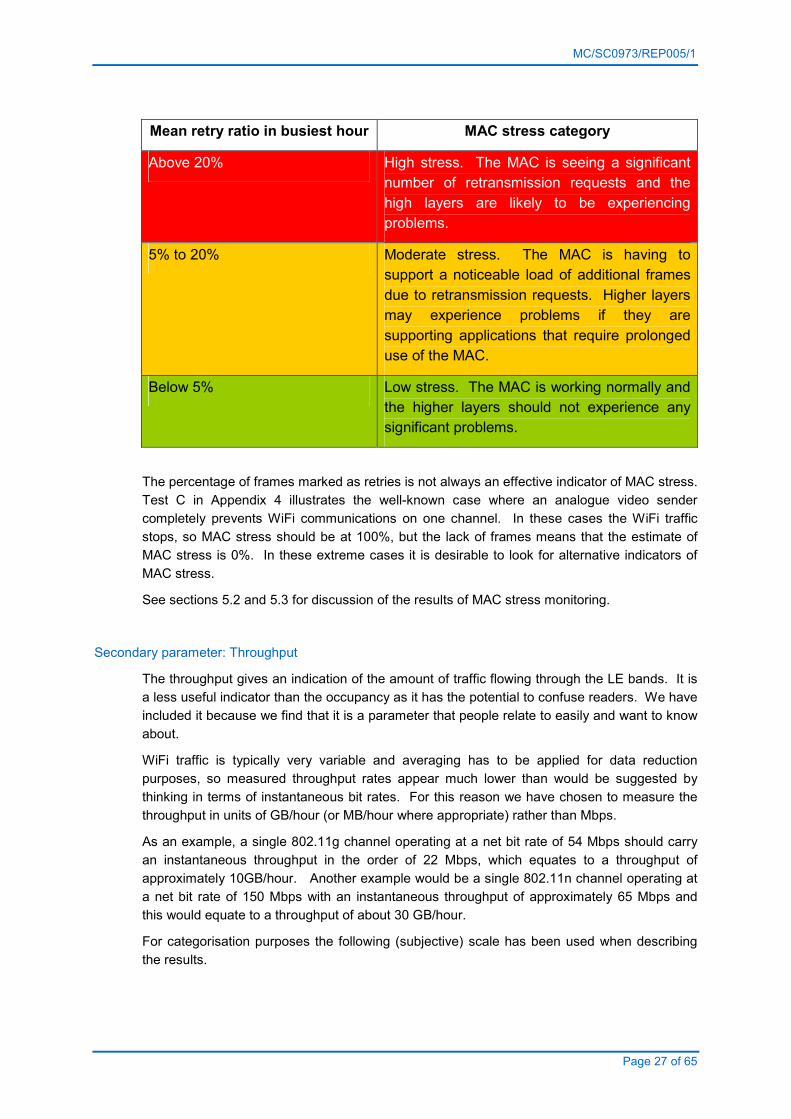
Categorisation is based on the busiest hour, which is defined here as the hour in which the
highest throughput is seen.
MC/SC0973/REP005/1
Page 27 of 65
Mean retry ratio in busiest hour MAC stress category
Above 20% High stress. The MAC is seeing a significant
number of retransmission requests and the
high layers are likely to be experiencing
problems.
5% to 20% Moderate stress. The MAC is having to
support a noticeable load of additional frames
due to retransmission requests. Higher layers
may experience problems if they are
supporting applications that require prolonged
use of the MAC.
Below 5% Low stress. The MAC is working normally and
the higher layers should not experience any
significant problems.
The percentage of frames marked as retries is not always an effective indicator of MAC stress.
Test C in Appendix 4 illustrates the well-known case where an analogue video sender
completely prevents WiFi communications on one channel. In these cases the WiFi traffic
stops, so MAC stress should be at 100%, but the lack of frames means that the estimate of
MAC stress is 0%. In these extreme cases it is desirable to look for alternative indicators of
MAC stress.
See sections 5.2 and 5.3 for discussion of the results of MAC stress monitoring.
Secondary parameter: Throughput
The throughput gives an indication of the amount of traffic flowing through the LE bands. It is
a less useful indicator than the occupancy as it has the potential to confuse readers. We have
included it because we find that it is a parameter that people relate to easily and want to know
about.
WiFi traffic is typically very variable and averaging has to be applied for data reduction
purposes, so measured throughput rates appear much lower than would be suggested by
thinking in terms of instantaneous bit rates. For this reason we have chosen to measure the
throughput in units of GB/hour (or MB/hour where appropriate) rather than Mbps.
As an example, a single 802.11g channel operating at a net bit rate of 54 Mbps should carry
an instantaneous throughput in the order of 22 Mbps, which equates to a throughput of
approximately 10GB/hour. Another example would be a single 802.11n channel operating at
a net bit rate of 150 Mbps with an instantaneous throughput of approximately 65 Mbps and
this would equate to a throughput of about 30 GB/hour.
For categorisation purposes the following (subjective) scale has been used when describing
the results.
MC/SC0973/REP005/1
Page 28 of 65
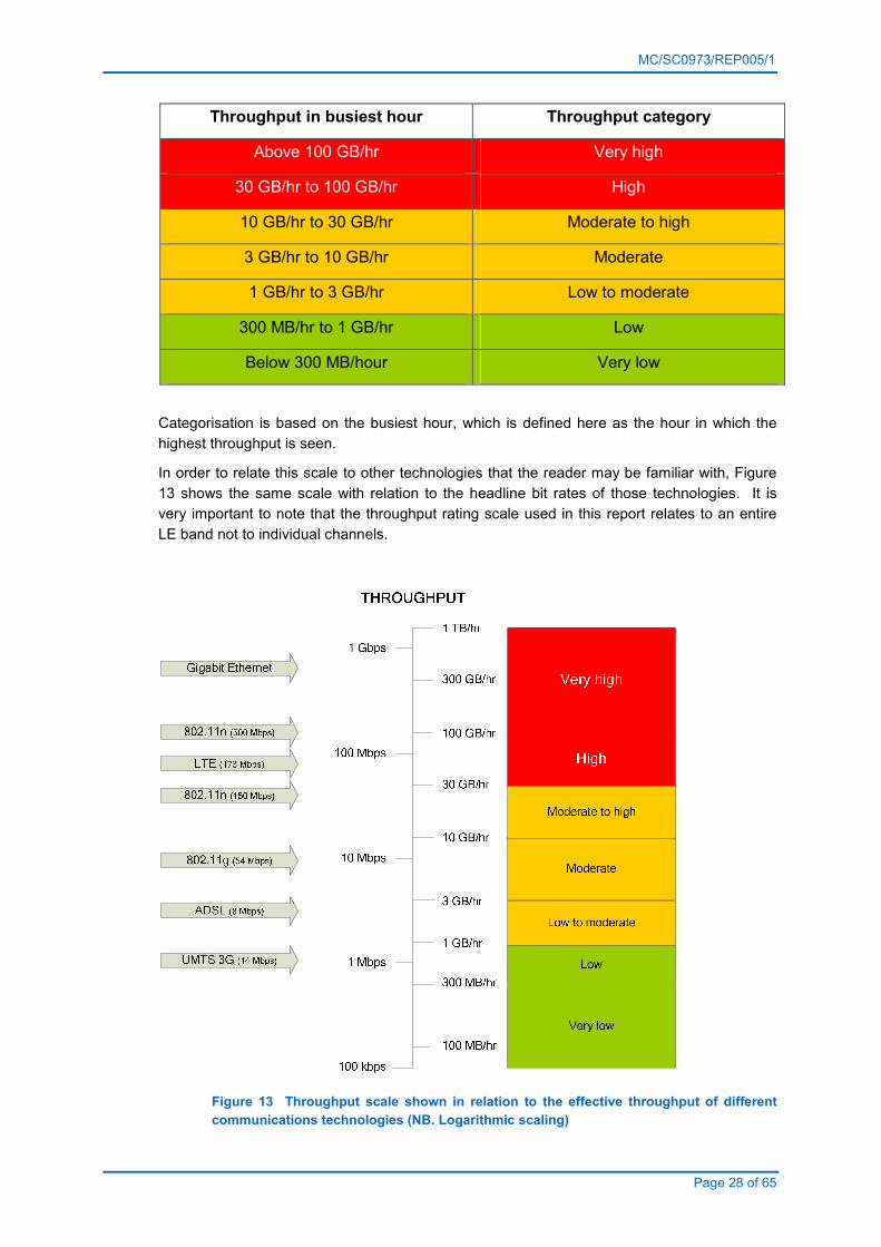
Throughput in busiest hour Throughput category
Above 100 GB/hr Very high
30 GB/hr to 100 GB/hr High
10 GB/hr to 30 GB/hr Moderate to high
3 GB/hr to 10 GB/hr Moderate
1 GB/hr to 3 GB/hr Low to moderate
300 MB/hr to 1 GB/hr Low
Below 300 MB/hour Very low
Categorisation is based on the busiest hour, which is defined here as the hour in which the
highest throughput is seen.
In order to relate this scale to other technologies that the reader may be familiar with, Figure
13 shows the same scale with relation to the headline bit rates of those technologies. It is
very important to note that the throughput rating scale used in this report relates to an entire
LE band not to individual channels.
Figure 13 Throughput scale shown in relation to the effective throughput of different
communications technologies (NB. Logarithmic scaling)
MC/SC0973/REP005/1
Page 29 of 65
The upper limits on throughput are hard to state as technology is evolving quickly. This is
another reason why it is difficult to use throughput as an indicator of spectrum utilisation.
See section 5.4 for discussion of the results of throughput monitoring.
Secondary parameter: Network density (number of APs)
The network density, given by the number of APs, is interesting as it shows how much
provision there is in an area for WiFi access. It does not, however, give any indication of the
amount of WiFi usage beyond the presence of beacon frames. Another problem with this
parameter is that there is no common standard for the received signal strength above which
APs are reported by a monitoring system, so it is currently hard to compare results between
systems.
A subjective scale for the number of APs could be based on the network geographic density.
Other studies have indicated typical densities that might be expected. Wong and Clement
(2006) described an average of 206 named networks per square kilometre as ‘fairly high’. In
our own work we have estimated network densities of up to 749 BSSID/channel/km2 at one
location in London (Wagstaff, 2009, p.114) and a median of around 400 BSSID/channel/km2
for all sites surveyed in London (Wagstaff, 2009, p.58). By contrast a ‘sparse’ network of APs
(in order of 1 BSSID/channel/km2) would be needed to support cellular offloading (Dimmateo
et al, 2011).
It is not possible to estimate a network density with confidence when surveying a site at a
fixed location, so for this report we have chosen to use the number of unique BSSIDs detected
by passive monitoring.
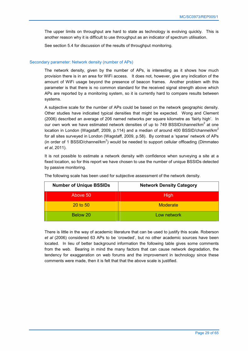
The following scale has been used for subjective assessment of the network density.
Number of Unique BSSIDs Network Density Category
Above 50 High
20 to 50 Moderate
Below 20 Low network
There is little in the way of academic literature that can be used to justify this scale. Roberson
et al (2006) considered 63 APs to be ‘crowded’, but no other academic sources have been
located. In lieu of better background information the following table gives some comments
from the web. Bearing in mind the many factors that can cause network degradation, the
tendency for exaggeration on web forums and the improvement in technology since these
comments were made, then it is felt that that the above scale is justified.

MC/SC0973/REP005/1
Page 30 of 65
APs Comment Reference
63 Crowded Roberson et al (2006)
53 Congested http://www.metageek.net/forums/showthread.php?4829-Way-Way-Too-Many-
Access-Points
45 Very slow https://supportforums.cisco.com/thread/334108
27 Pretty brutal http://forums.redflagdeals.com/archive/index.php/t-1153207.html
24 Slowness http://www.dslreports.com/forum/r27059926-Is-24-AP-s-in-one-area-too-many-
20-50 Low bandwidth http://www.zdnet.com/blog/datacenter/too-many-mobile-wireless-hotspots-makes-
for-a-bad-day/994
15-25 Pretty crowded http://forums.redflagdeals.com/archive/index.php/t-1153207.html
20+ Almost
impossible
http://ask.slashdot.org/story/09/01/17/0431239/how-best-to-deal-with-wifi-
interference
13-16 No connectivity http://forums.wi-fiplanet.com/showthread.php?6136-Too-many-access-points-in-
apartment-complex
10+ Only 1Mbps http://www.lovemytool.com/blog/2011/03/wireless-overkill-can-cause-poor-
performance-by-chris-greer.html
10 Pretty good http://forums.redflagdeals.com/archive/index.php/t-1153207.html
9 Lagging &
intermittent
http://www.wirelessforums.org/network-troubleshooting/too-many-wireless-networks-
ruining-mine-82563.html
6 Pretty good http://forums.redflagdeals.com/archive/index.php/t-1153207.html
5-10 Problems http://forums.overclockers.com.au/showthread.php?t=877953
1 Great http://forums.redflagdeals.com/archive/index.php/t-1153207.html
See section 5.5 for discussion of the results of network density monitoring.
4.4 Laboratory tests
The laboratory tests carried out in this study concentrated on addressing the following questions:
1. Do the receivers work as expected and deliver reliable, accurate data?
The conclusions of these tests were that the receivers are delivering reliable data,
although the lack of power calibration means that the absolute power level readings
should be taken as indicative only. Other parameters, such as time, can be regarded
as accurate enough for the purposes of this system.
It was found that the WiSpy dongle could be overloaded, with noticeable impacts on
the observed spectrum when the input signal level reached -10dBm. No additional
prefiltering or power limiting modifications have been made, so care should be taken
when placing the test equipment to avoid excessive signal levels from nearby
transmissions that could adversely affect measurements (including any possible
strong out of band interferers).
Three major problems were identified with the AirPcap Nx dongle that made it difficult
to use for this study and workarounds had to be devised. These were in the form of
additional algorithms in the post-processing software. The problems were:
(a) ‘Ghost’ APs. The dongle reports frames from APs on adjacent channels. These
can be removed by looking for APs that appear on channels other than the primary
one, as identified by the observed bit rate;

MC/SC0973/REP005/1
Page 31 of 65
(b) Whilst the dongle captures 802.11n frames, it does not report all the details
correctly in the RadioTap header. Workarounds have been developed which involve
looking at the length of beacon frames to identify APs working in 802.11n;
(c) The dongle can only operate in 20 MHz or 40 MHz mode. It cannot report on both
simultaneously. The 20 MHz mode was used throughout the study as this is by far the
most common WiFi bandwidth currently in use.
With these workarounds in place the monitoring system reported the primary and
secondary parameters correctly.
2. Is it possible to make any inference about the user experience from observations at the physical
or link layer?
It was concluded that the design constraints placed on the system prevent it from
being able to give clear indications of user experience. In particular, it is not possible
to look at the layers above the MAC, so the user traffic cannot be observed directly.
Our approach has been to use the number of retry frames as an indicator of MAC
stress and thereby infer potential problems in the higher layers.
The primary and secondary parameters should be interpreted as indicators of the
state of the MAC. The MAC may be adversely affected by numerous factors in the
PHY as well as issues within itself, but it is not aware of events in the higher layers.

MC/SC0973/REP005/1
Page 32 of 65
3. Can the degradation of WiFi networks due to the use of overlapping channels in the 2.4 GHz
band be observed and measured?
A set of stress tests were carried out by Ofcom and are documented in Appendix 4. It
was possible to observe the effects of operating on overlapping channels and the
results tend to support the general advice to use non-overlapping channels wherever
possible and, if not possible, then to avoid partially overlapping channels.
4.5 Field surveys
The field surveys were carried out by Ofcom staff from the Baldock site. They selected the sites and
arranged for the equipment to be installed, then returned measurement data to MASS for analysis.
After some internal debate it was decided to place the surveys into four groups. Alternative groups
are possible but, at the current time, there is insufficient data to reliably choose any of these
alternatives.
Number of sites
Coarse resolution Fine resolution
Houses 13 1
Apartments 9 1
Cafés 12 1
Shopping centres 4 1
Total 38 4

MC/SC0973/REP005/1
Page 33 of 65
5 RESULTS
This section gives the main findings of the study. As with the 2009 work (Wagstaff, 2009) the main
objective has been to look at parameters that indicate the levels of utilisation and degradation.
Appendix 1 gives the detailed results of all the surveys using the graphical representations introduced
in section 4.2.
The addition of PHY monitoring in this study has added to the number of potential measurement
metrics that could be defined, so there has been the possibility of obtaining a richer picture of LE band
usage at the same time as generating more data that has to be interpreted. As described in section
4.3 it has been necessary to select a small number of parameters to summarise the findings.
This section looks first at the two primary parameters (occupancy and MAC stress), then at the two
secondary parameters (network density and throughput). It then discusses the issues of degradation
with specific examples to illustrate the conclusions of the study. Finally the results of fine time
resolution monitoring are given.
MC/SC0973/REP005/1
Page 34 of 65
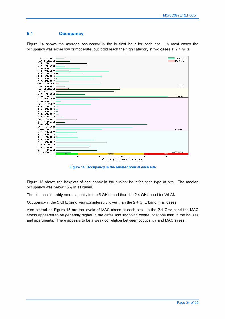
5.1 Occupancy
Figure 14 shows the average occupancy in the busiest hour for each site. In most cases the
occupancy was either low or moderate, but it did reach the high category in two cases at 2.4 GHz.
Low ModerateApartments
High
Figure 14 Occupancy in the busiest hour at each site
Figure 15 shows the boxplots of occupancy in the busiest hour for each type of site. The median
occupancy was below 15% in all cases.
There is considerably more capacity in the 5 GHz band than the 2.4 GHz band for WLAN.
Occupancy in the 5 GHz band was considerably lower than the 2.4 GHz band in all cases.
Also plotted on Figure 15 are the levels of MAC stress at each site. In the 2.4 GHz band the MAC
stress appeared to be generally higher in the cafés and shopping centre locations than in the houses
and apartments. There appears to be a weak correlation between occupancy and MAC stress.

MC/SC0973/REP005/1
Page 35 of 65
Figure 15 Boxplots of occupancy for each type of site in the busiest hour
Before moving onto the other primary and secondary parameters it is worth revisiting the usefulness of
the frame rate. This was used in the earlier study (Wagstaff, 2009) to indicate how much the 2.4 GHz
band was being used. It is clearly a useful parameter for this purpose and relegating its use in favour
of occupancy needs some justification.
In the following graphs the average frame rate has been plotted against the occupancy for all the data
at all the sites surveyed. There is a good correlation, strongly suggesting that the occupancy is
dominated by the presence of WiFi traffic.
The graphs also provide evidence to support the assertion that occupancy is a more useful metric than
frame rate. Occupancy can be used to look for interference from non-WiFi services in the LE bands
by visual inspection of the spectrum plots, time plots and spectrograms. The frame rate cannot be
used for this purpose.

MC/SC0973/REP005/1
Page 36 of 65
Occupancy v. No Frames 2.4GHz
0
50000
100000
150000
200000
250000
0 1 2 3 4 5 6 7 8 9
Occupancy
Num of frames
Occupancy v. No Frames 5GHz
0
50000
100000
150000
200000
250000
300000
350000
0 0.2 0.4 0.6 0.8 1 1.2
Occupancy
Number of frames
numFrames
Figure 16 Average frame rate versus occupancy for all the sites in this survey
There are some cases in the 2.4 GHz band where the frame rate is low but the occupancy is high.
These are believed to be cases where interference from other services existed. A good example is
the elevated noise floor at the house monitored in survey S36. Using occupancy as a primary
parameter rather than frame rate has the benefit of indicating the proportion of the band capacity used
(in terms of time available) incorporating all services, not just WiFi.
Conclusions on occupancy
We conclude that the occupancy of the 2.4 GHz band is typically about 3% (low) and the 5 GHz band
around 0.3% (low) when averaged across the entire day. If just the busiest hour is of interest then the
occupancy is typically much higher and the median is in the order of 10% (moderate) in the 2.4 GHz
band and 1% (low) in the 5 GHz band. At some sites the occupancy is expected to reach 30% (high).

MC/SC0973/REP005/1
Page 37 of 65
5.2 MAC stress
Figure 17 shows the MAC stress levels at each location in the busiest hours. It is evident that there is
a tendency for it to be higher in cafés and shopping centres than in houses and apartments. This is
especially so in the 5 GHz band, where moderate levels of MAC stress were only seen in the cafés
and shopping centres.
Low ModerateApartments
High
Figure 17 MAC stress levels for each location in the busiest hours
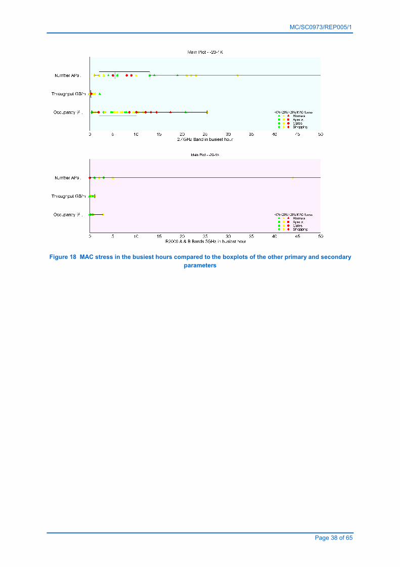
Figure 18 shows the MAC stress compared to the boxplots of the other primary parameters. Both
diagrams are in terms of the busiest hour statistics.
There is very little correlation between the MAC stress and the other primary and secondary
parameters. It can, however, be seen that the MAC stress tends to be higher in the upper quartile of
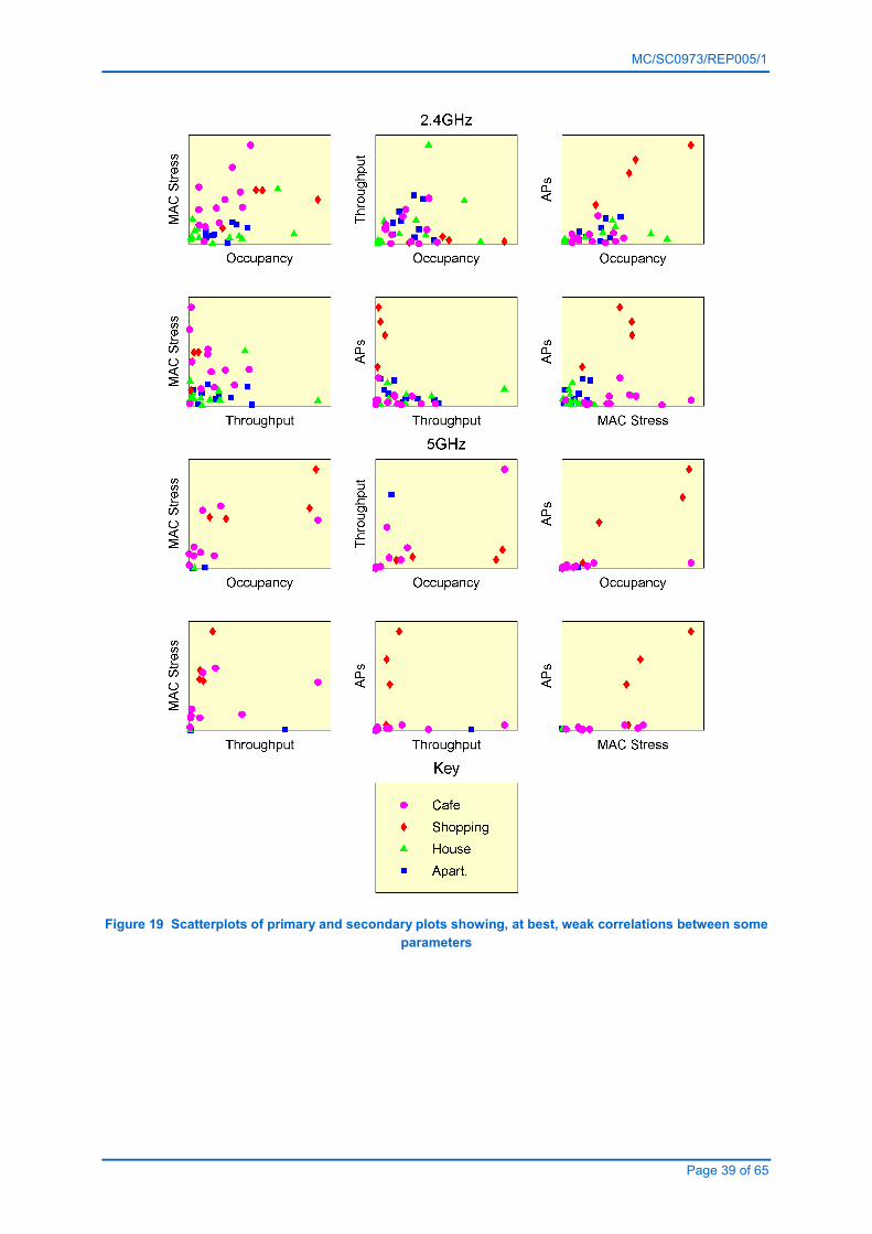
the occupancy in the 2.4 GHz band. This is supported in the analysis of Figure 19 which shows all the
possible correlations between the primary and secondary parameters and from which it can be seen
that there is only a weak correlation between MAC stress and occupancy.
MC/SC0973/REP005/1
Page 38 of 65
Figure 18 MAC stress in the busiest hours compared to the boxplots of the other primary and secondary
parameters
MC/SC0973/REP005/1
Page 39 of 65
Figure 19 Scatterplots of primary and secondary plots showing, at best, weak correlations between some
parameters
MC/SC0973/REP005/1
Page 40 of 65
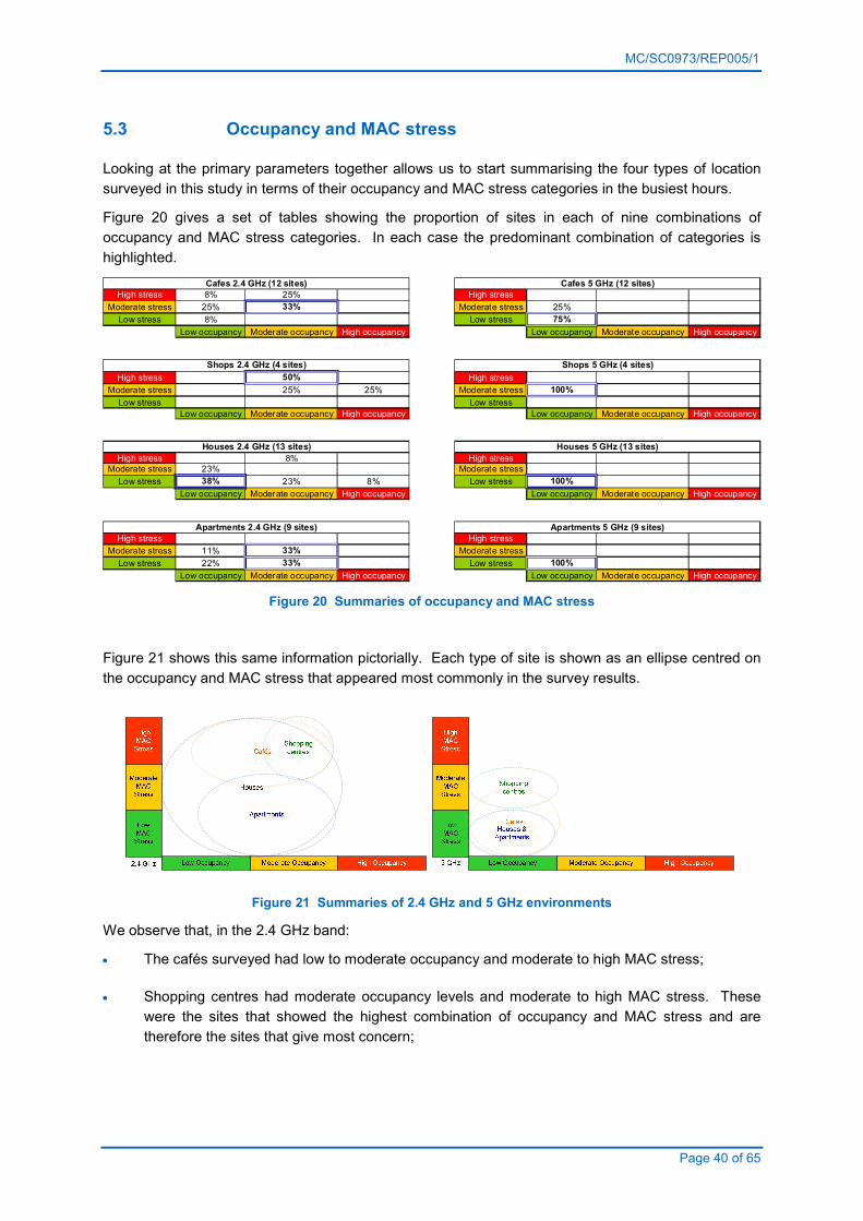
5.3 Occupancy and MAC stress
Looking at the primary parameters together allows us to start summarising the four types of location
surveyed in this study in terms of their occupancy and MAC stress categories in the busiest hours.
Figure 20 gives a set of tables showing the proportion of sites in each of nine combinations of
occupancy and MAC stress categories. In each case the predominant combination of categories is
highlighted.
High stress 8% 25% High stress
Moderate stress 25% 33% Moderate stress 25%
Low stress 8% Low stress 75%
Low occupancy Moderate occupancy High occupancy Low occupancy Moderate occupancy High occupancy
High stress 50% High stress
Moderate stress 25% 25% Moderate stress 100%
Low stress Low stress
Low occupancy Moderate occupancy High occupancy Low occupancy Moderate occupancy High occupancy
High stress 8% High stress
Moderate stress 23% Moderate stress
Low stress 38% 23% 8% Low stress 100%
Low occupancy Moderate occupancy High occupancy Low occupancy Moderate occupancy High occupancy
High stress High stress
Moderate stress 11% 33% Moderate stress
Low stress 22% 33% Low stress 100%
Low occupancy Moderate occupancy High occupancy Low occupancy Moderate occupancy High occupancy
Houses 2.4 GHz (13 sites) Houses 5 GHz (13 sites)
Apartments 2.4 GHz (9 sites) Apartments 5 GHz (9 sites)
Cafes 2.4 GHz (12 sites) Cafes 5 GHz (12 sites)
Shops 2.4 GHz (4 sites) Shops 5 GHz (4 sites)
Figure 20 Summaries of occupancy and MAC stress
Figure 21 shows this same information pictorially. Each type of site is shown as an ellipse centred on
the occupancy and MAC stress that appeared most commonly in the survey results.
Figure 21 Summaries of 2.4 GHz and 5 GHz environments
We observe that, in the 2.4 GHz band:
• The cafés surveyed had low to moderate occupancy and moderate to high MAC stress;
• Shopping centres had moderate occupancy levels and moderate to high MAC stress. These
were the sites that showed the highest combination of occupancy and MAC stress and are
therefore the sites that give most concern;

MC/SC0973/REP005/1
Page 41 of 65
• Houses had generally low occupancy but moderate and high levels were also seen. The MAC
stress was similarly low in most cases but moderate and high levels of MAC stress were
observed;
• The apartments were similar to the houses. They had low to moderate levels of both primary
parameters.
The 5 GHz band was much quieter than the 2.4 GHz band with low levels of occupancy at all the
locations. The MAC stress levels were slightly higher in the shopping centres and cafés than the
houses and apartments.
5.4 Throughput
5.4.1 Throughput test results
In a series of laboratory tests the capability of the MAC to support a number of video streams has
been investigated. The following table summarises the results obtained in a relatively quiet radio
environment.
802.11g 802.11n
‘Headline’ data rate 54 Mbps 150 Mbps (Note 1)
Maximum TCP throughput 22 Mbps 53 Mbps downstream
70 Mbps upstream
Number of High Definition (3.2 Mbps) video streams
6 14+
(Note 1 – Whilst the standard allows data rates up to 600 Mbps the testing here was performed using a mode that can be
considered more typical of the environments surveyed.)
These results accord with the results in the literature. It was found that the best results are obtained
when the AP and client dongles were from the same manufacturer.
In another test a domestic arrangement in a four bedroom detached house was investigated. At that
location the average ADSL download rate available was 4.5 Mbps. It was possible to stream a single
television channel from the BBC iPlayer site in either SD mode at a median rate of 1.3 Mbps or in HD
mode at a median rate of 2.5 Mbps. This was achieved over Ethernet, powerline and WiFi from a
router at 3m range in 802.11g mode. It was found that the adaptive rate capability of the BBC iPlayer
meant that different speeds were achieved for different programmes and that it could take several
minutes for a steady state rate to be measurable.
5.4.2 Survey results for throughput
Figure 22 shows the survey results for the throughput in the busiest hour at each site. The throughput
was very low, low or low to moderate, with the peak value in the busiest hour being lower than 3 GB/hr
at all sites surveyed and the average being less than half of this.
The highest throughput values were seen in residential locations and the lowest at the shopping
centres.
Higher throughput overall was observed in the 2.4 GHz band rather than 5 GHz.

MC/SC0973/REP005/1
Page 42 of 65
LowApartments
Low to moderateVery low
Figure 22 Throughput in busiest hour at each site
Figure 23 gives the boxplots of the throughput for each type of site in the busiest hour. In all cases
the median was below 1 GB/hr, which is regarded as low according to the scale used here (Figure 13).
In the 2.4 GHz band the greatest variability in throughput was seen in the houses surveyed. These
have the lowest median but also the highest upper bound to the boxplot. In the 5 GHz band the
picture was different as the houses showed very little use of this band and it was the café sites that
exhibited the greatest variability in throughput.
MAC stress levels are also shown on the boxplots in Figure 23. It will be seen that MAC stress does
not correlate with the throughput, rather it tends to correlate more with the type of site. The MAC
stress is generally higher in the cafés and shopping centres than the houses and apartments.

MC/SC0973/REP005/1
Page 43 of 65
Figure 23 Boxplots of throughput for each type of site
Figure 24 shows another representation of the busy hour throughput results, this time against the
MAC stress and occupancy in a grid. The types of site are indicated by the shapes and the
throughput colour scale is used for the colours of those shapes. This representation emphasises that
throughput was generally observed to be low and there is no obvious correlation with the two primary
parameters.
Figure 24 Throughput versus occupancy and MAC stress, 2.4 GHz, busy hour

MC/SC0973/REP005/1
Page 44 of 65
5.5 Network density
The number of APs was noticeably higher in some of the public locations compared to residential
locations.
Figure 25 shows the network densities for all the locations in this study. It is immediately apparent
that there were more APs in the shopping centres than the other locations. The reader should bear in
mind, though, that only four shopping centre sites were surveyed and other shopping centres can be
expected to have very different WiFi installations.
The large number of 5 GHz APs at three of the four shopping centre sites is particularly notable and
we believe that these are part of a managed WiFi system. Other shopping centres may not have this
kind of infrastructure and so would not exhibit such a large number of APs.
Low ModerateApartments
High
Figure 25 Network density in busiest hour at each location
When the boxplots of the network density are plotted for each site type (Figure 26) then the median
number of APs can be seen to be less than ten for all groups except the shopping centre sites. This
group is distinct in having a large number of APs with around 60 in both LE bands.

MC/SC0973/REP005/1
Page 45 of 65
Figure 26 also shows the MAC stress levels compared to the boxplots of the numbers of APs. High
levels of MAC stress occur when the network density is low and also when it is higher. The MAC
stress does not appear to be well correlated with this parameter. Even though there may be a lot of
WiFi infrastructure present in the environment there is little to suggest from this representation that
higher network density implies the MAC will be stressed.
Figure 26 Boxplots of network density for each type of site
Figure 27 shows another representation of the busy hour statistics. It is similar to Figure 24 but this
time drawn for the network density.
This representation emphasises the fact that the network density in the busy hour was low in most of
the surveys.
The moderate and high levels of network density never occurred in areas of low occupancy and never
occurred in areas of low MAC stress. Also they always occurred in cafés or shopping centres, i.e. the
public places.
Two outliers have been highlighted in the callouts on Figure 27. These are a café and a house at
which non-WiFi interference was observed. It is not possible to clearly separate out the effects of
different kinds of interference completely, but these two outliers do help to illustrate the fact that the
radio environment is rich and complex and different kinds of interference will skew the distributions of
parameters in different ways.

MC/SC0973/REP005/1
Page 46 of 65
Moderate OccupancyLow Occupancy High Occupancy
Low
MAC
Stress
Moderate
MAC
Stress
High
MAC
Stress
2.4 GHz
Cafés
Shopping
centres
Houses
Apartments
Network density
L M H
Survey S36
Raised noise floor due to
non-WiFi interference
Survey S02
Comb-like, non-WiFi
interference
High network density in
shopping centres may be
due to tethering
Figure 27 Network density versus occupancy and MAC stress, 2.4 GHz, busy hour

MC/SC0973/REP005/1
Page 47 of 65
5.6 Interference from services other than WiFi
The spectrogram plots for the level exceeded 0.1% of the time in the hour block were examined to
attempt to locate interference from services other than WiFi. This type of plot allows interference at
any frequency and of very short duration (> 3.6s approx) to be visible.
Only a small number of plots show any sign of interference and in every case this is in the 2.4 GHz
band.
As an example survey S06 shows what appears to be Bluetooth in one hour only. Note that the
broadband signal is limited to the 2,400MHz to 2,483MHz range and that the plot extends to
2,500MHz allowing the upper frequency edge of the signal to be visible.
Survey S36 shows another example, in this case of broad band noise of an unknown type that
appears to be spread across all frequencies.
The overall conclusion is that interference from other services is limited to relatively few examples.
Interference from non-WiFi sources has not been observed to be a major factor in the results of this
study.
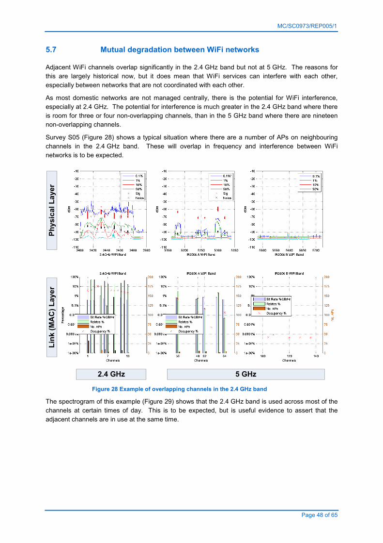
MC/SC0973/REP005/1
Page 48 of 65
5.7 Mutual degradation between WiFi networks
Adjacent WiFi channels overlap significantly in the 2.4 GHz band but not at 5 GHz. The reasons for
this are largely historical now, but it does mean that WiFi services can interfere with each other,
especially between networks that are not coordinated with each other.
As most domestic networks are not managed centrally, there is the potential for WiFi interference,
especially at 2.4 GHz. The potential for interference is much greater in the 2.4 GHz band where there
is room for three or four non-overlapping channels, than in the 5 GHz band where there are nineteen
non-overlapping channels.
Survey S05 (Figure 28) shows a typical situation where there are a number of APs on neighbouring
channels in the 2.4 GHz band. These will overlap in frequency and interference between WiFi
networks is to be expected.
2.4 GHz 5 GHz
Physical Layer
Link (MAC) Layer
Figure 28 Example of overlapping channels in the 2.4 GHz band
The spectrogram of this example (Figure 29) shows that the 2.4 GHz band is used across most of the
channels at certain times of day. This is to be expected, but is useful evidence to assert that the
adjacent channels are in use at the same time.
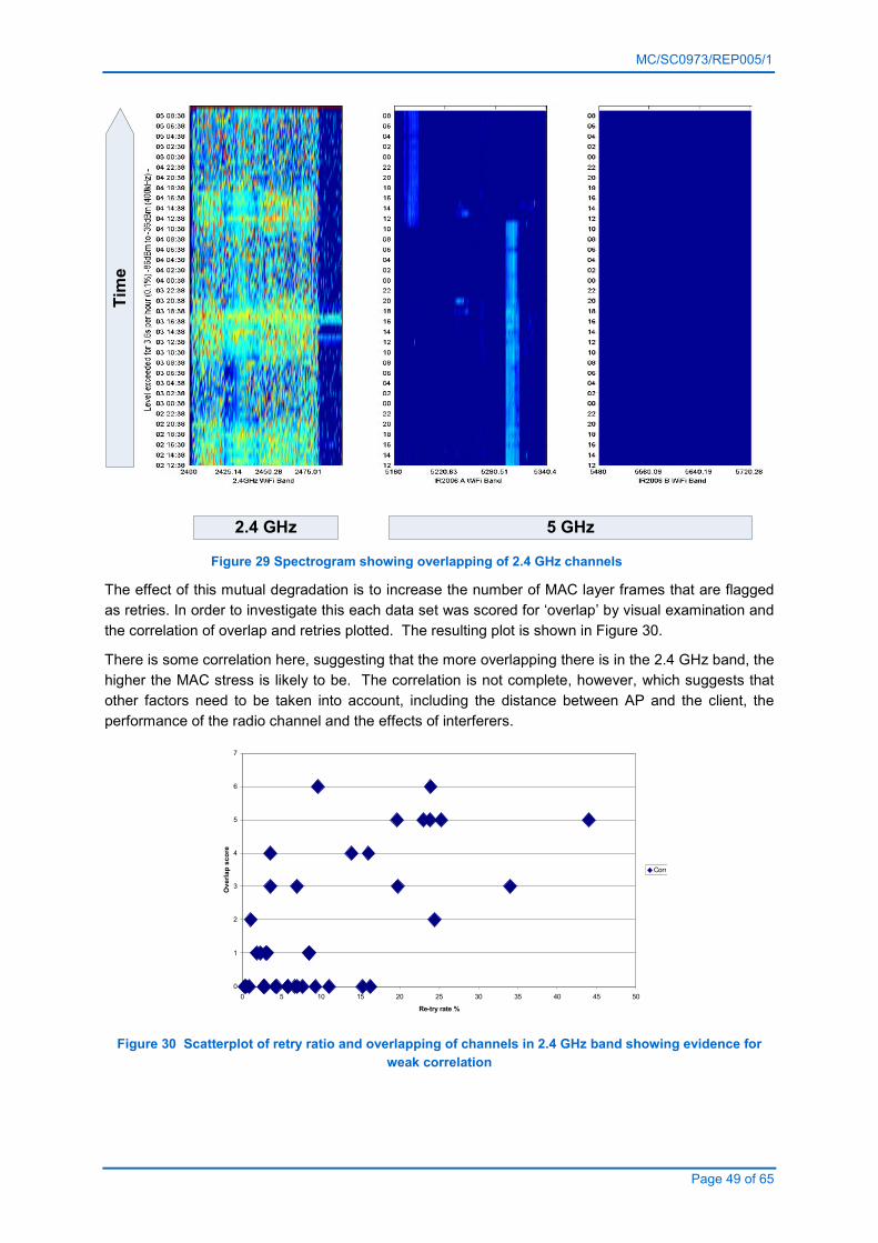
MC/SC0973/REP005/1
Page 49 of 65
2.4 GHz 5 GHz
Tim
e
Figure 29 Spectrogram showing overlapping of 2.4 GHz channels
The effect of this mutual degradation is to increase the number of MAC layer frames that are flagged
as retries. In order to investigate this each data set was scored for ‘overlap’ by visual examination and
the correlation of overlap and retries plotted. The resulting plot is shown in Figure 30.
There is some correlation here, suggesting that the more overlapping there is in the 2.4 GHz band, the
higher the MAC stress is likely to be. The correlation is not complete, however, which suggests that
other factors need to be taken into account, including the distance between AP and the client, the
performance of the radio channel and the effects of interferers.
0
1
2
3
4
5
6
7
0 5 10 15 20 25 30 35 40 45 50
Re-try rate %
Overlap score
Correlation
Figure 30 Scatterplot of retry ratio and overlapping of channels in 2.4 GHz band showing evidence for
weak correlation
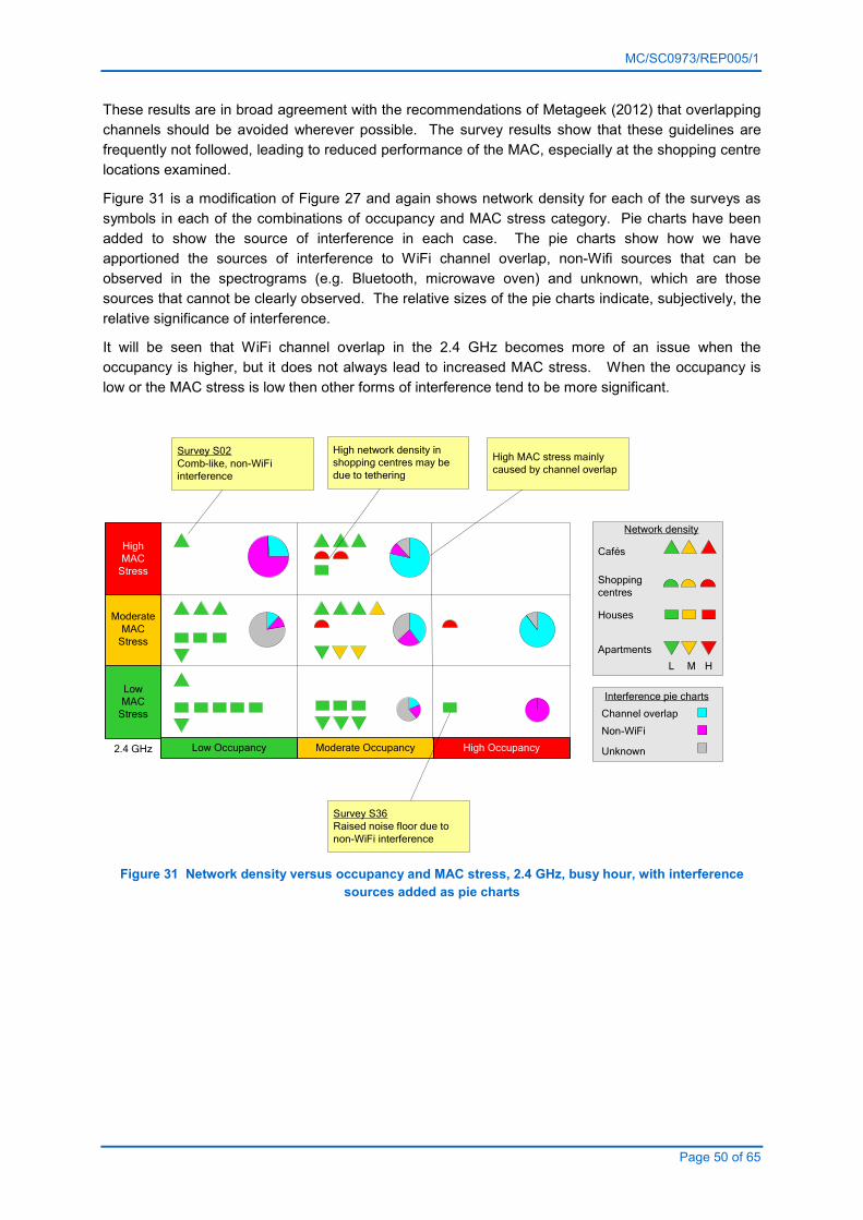
MC/SC0973/REP005/1
Page 50 of 65
These results are in broad agreement with the recommendations of Metageek (2012) that overlapping
channels should be avoided wherever possible. The survey results show that these guidelines are
frequently not followed, leading to reduced performance of the MAC, especially at the shopping centre
locations examined.
Figure 31 is a modification of Figure 27 and again shows network density for each of the surveys as
symbols in each of the combinations of occupancy and MAC stress category. Pie charts have been
added to show the source of interference in each case. The pie charts show how we have
apportioned the sources of interference to WiFi channel overlap, non-Wifi sources that can be
observed in the spectrograms (e.g. Bluetooth, microwave oven) and unknown, which are those
sources that cannot be clearly observed. The relative sizes of the pie charts indicate, subjectively, the
relative significance of interference.
It will be seen that WiFi channel overlap in the 2.4 GHz becomes more of an issue when the
occupancy is higher, but it does not always lead to increased MAC stress. When the occupancy is
low or the MAC stress is low then other forms of interference tend to be more significant.
Moderate OccupancyLow Occupancy High Occupancy
Low
MAC
Stress
Moderate
MAC
Stress
High
MAC
Stress
2.4 GHz
Cafés
Shopping
centres
Houses
Apartments
Network density
L M H
Survey S36
Raised noise floor due to
non-WiFi interference
Survey S02
Comb-like, non-WiFi
interference
Interference pie charts
Channel overlap
Non-WiFi
Unknown
High network density in
shopping centres may be
due to tethering
High MAC stress mainly
caused by channel overlap
Figure 31 Network density versus occupancy and MAC stress, 2.4 GHz, busy hour, with interference
sources added as pie charts
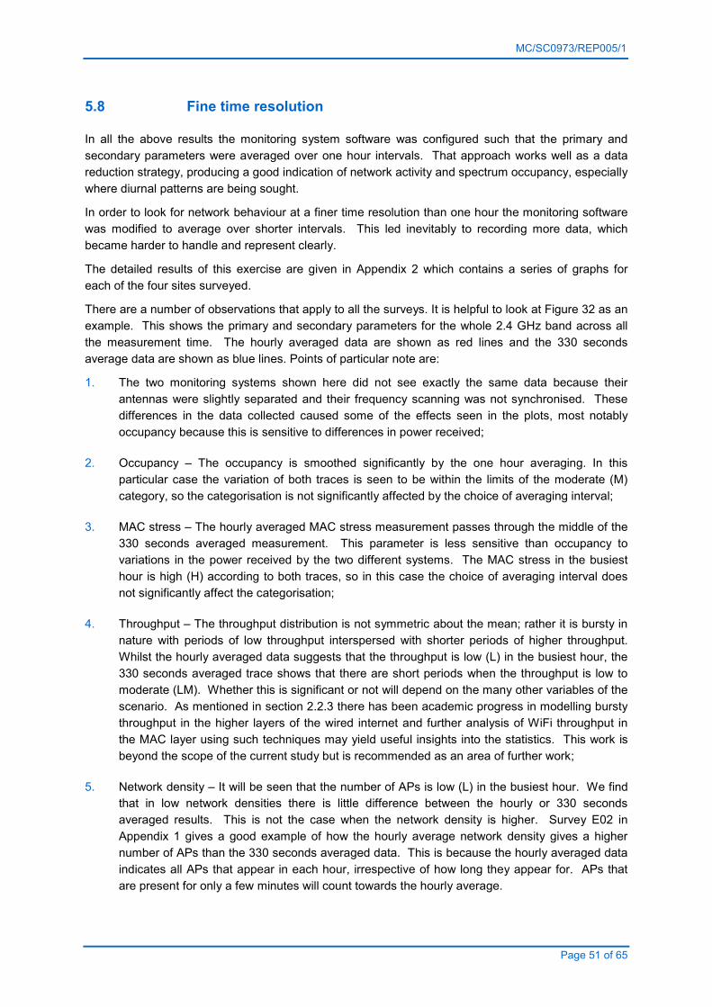
MC/SC0973/REP005/1
Page 51 of 65
5.8 Fine time resolution
In all the above results the monitoring system software was configured such that the primary and
secondary parameters were averaged over one hour intervals. That approach works well as a data
reduction strategy, producing a good indication of network activity and spectrum occupancy, especially
where diurnal patterns are being sought.
In order to look for network behaviour at a finer time resolution than one hour the monitoring software
was modified to average over shorter intervals. This led inevitably to recording more data, which
became harder to handle and represent clearly.
The detailed results of this exercise are given in Appendix 2 which contains a series of graphs for
each of the four sites surveyed.
There are a number of observations that apply to all the surveys. It is helpful to look at Figure 32 as an
example. This shows the primary and secondary parameters for the whole 2.4 GHz band across all
the measurement time. The hourly averaged data are shown as red lines and the 330 seconds
average data are shown as blue lines. Points of particular note are:
1. The two monitoring systems shown here did not see exactly the same data because their
antennas were slightly separated and their frequency scanning was not synchronised. These
differences in the data collected caused some of the effects seen in the plots, most notably
occupancy because this is sensitive to differences in power received;
2. Occupancy – The occupancy is smoothed significantly by the one hour averaging. In this
particular case the variation of both traces is seen to be within the limits of the moderate (M)
category, so the categorisation is not significantly affected by the choice of averaging interval;
3. MAC stress – The hourly averaged MAC stress measurement passes through the middle of the
330 seconds averaged measurement. This parameter is less sensitive than occupancy to
variations in the power received by the two different systems. The MAC stress in the busiest
hour is high (H) according to both traces, so in this case the choice of averaging interval does
not significantly affect the categorisation;
4. Throughput – The throughput distribution is not symmetric about the mean; rather it is bursty in
nature with periods of low throughput interspersed with shorter periods of higher throughput.
Whilst the hourly averaged data suggests that the throughput is low (L) in the busiest hour, the
330 seconds averaged trace shows that there are short periods when the throughput is low to
moderate (LM). Whether this is significant or not will depend on the many other variables of the
scenario. As mentioned in section 2.2.3 there has been academic progress in modelling bursty
throughput in the higher layers of the wired internet and further analysis of WiFi throughput in
the MAC layer using such techniques may yield useful insights into the statistics. This work is
beyond the scope of the current study but is recommended as an area of further work;
5. Network density – It will be seen that the number of APs is low (L) in the busiest hour. We find
that in low network densities there is little difference between the hourly or 330 seconds
averaged results. This is not the case when the network density is higher. Survey E02 in
Appendix 1 gives a good example of how the hourly average network density gives a higher
number of APs than the 330 seconds averaged data. This is because the hourly averaged data
indicates all APs that appear in each hour, irrespective of how long they appear for. APs that
are present for only a few minutes will count towards the hourly average.
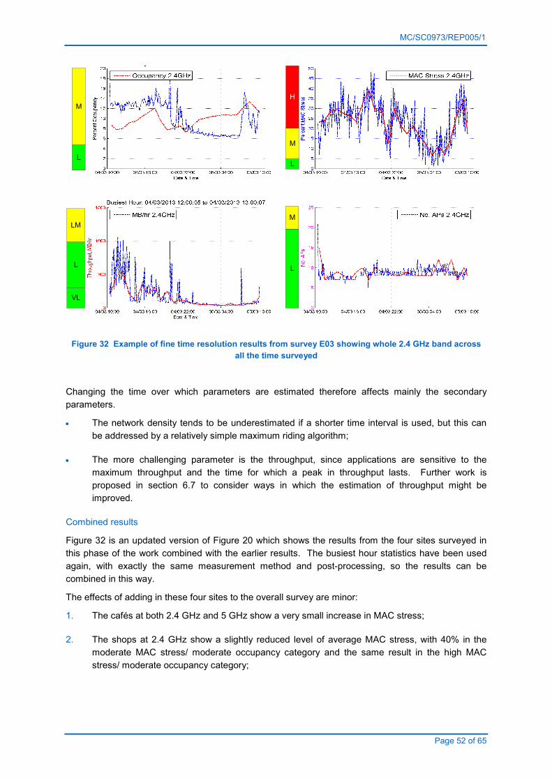
MC/SC0973/REP005/1
Page 52 of 65
L
M
L
M
H
L
LM
VL
L
M
Figure 32 Example of fine time resolution results from survey E03 showing whole 2.4 GHz band across
all the time surveyed
Changing the time over which parameters are estimated therefore affects mainly the secondary
parameters.
• The network density tends to be underestimated if a shorter time interval is used, but this can
be addressed by a relatively simple maximum riding algorithm;
• The more challenging parameter is the throughput, since applications are sensitive to the
maximum throughput and the time for which a peak in throughput lasts. Further work is
proposed in section 6.7 to consider ways in which the estimation of throughput might be
improved.
Combined results
Figure 32 is an updated version of Figure 20 which shows the results from the four sites surveyed in
this phase of the work combined with the earlier results. The busiest hour statistics have been used
again, with exactly the same measurement method and post-processing, so the results can be
combined in this way.
The effects of adding in these four sites to the overall survey are minor:
1. The cafés at both 2.4 GHz and 5 GHz show a very small increase in MAC stress;
2. The shops at 2.4 GHz show a slightly reduced level of average MAC stress, with 40% in the
moderate MAC stress/ moderate occupancy category and the same result in the high MAC
stress/ moderate occupancy category;
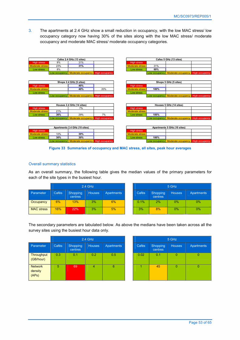
MC/SC0973/REP005/1
Page 53 of 65
3. The apartments at 2.4 GHz show a small reduction in occupancy, with the low MAC stress/ low
occupancy category now having 30% of the sites along with the low MAC stress/ moderate
occupancy and moderate MAC stress/ moderate occupancy categories.
High stress 8% 31% High stress
Moderate stress 23% 31% Moderate stress 31%
Low stress 8% Low stress 69%
Low occupancy Moderate occupancy High occupancy Low occupancy Moderate occupancy High occupancy
High stress 40% High stress
Moderate stress 40% 20% Moderate stress 100%
Low stress Low stress
Low occupancy Moderate occupancy High occupancy Low occupancy Moderate occupancy High occupancy
High stress 7% High stress
Moderate stress 21% Moderate stress
Low stress 36% 29% 7% Low stress 100%
Low occupancy Moderate occupancy High occupancy Low occupancy Moderate occupancy High occupancy
High stress High stress
Moderate stress 10% 30% Moderate stress
Low stress 30% 30% Low stress 100%
Low occupancy Moderate occupancy High occupancy Low occupancy Moderate occupancy High occupancy
Houses 2.4 GHz (14 sites) Houses 5 GHz (14 sites)
Apartments 2.4 GHz (10 sites) Apartments 5 GHz (10 sites)
Cafes 2.4 GHz (13 sites) Cafes 5 GHz (13 sites)
Shops 2.4 GHz (5 sites) Shops 5 GHz (5 sites)
Figure 33 Summaries of occupancy and MAC stress, all sites, peak hour averages
Overall summary statistics
As an overall summary, the following table gives the median values of the primary parameters for
each of the site types in the busiest hour.
2.4 GHz 5 GHz
Parameter Cafés Shopping centres
Houses Apartments Cafés Shopping centres
Houses Apartments
Occupancy 6% 13% 3% 6% 0.1% 2% 0% 0%
MAC stress 16% 22% 3% 5% 3% 8% 0% 0%
The secondary parameters are tabulated below. As above the medians have been taken across all the
survey sites using the busiest hour data only.
2.4 GHz 5 GHz
Parameter Cafés Shopping centres
Houses Apartments Cafés Shopping centres
Houses Apartments
Throughput
(GB/hour)
0.3 0.1 0.2 0.5 0.02 0.1 0 0
Network
density
(APs)
5 69 4 6 1 45 0 0
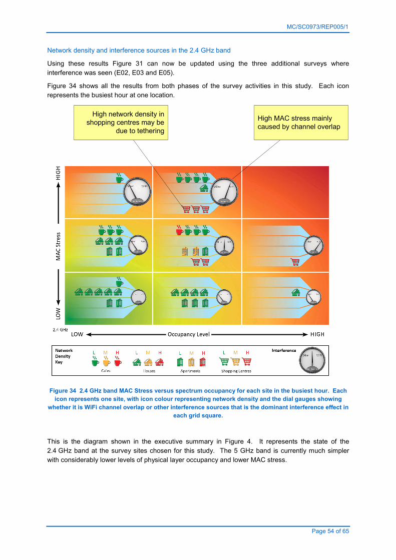
MC/SC0973/REP005/1
Page 54 of 65
Network density and interference sources in the 2.4 GHz band
Using these results Figure 31 can now be updated using the three additional surveys where
interference was seen (E02, E03 and E05).
Figure 34 shows all the results from both phases of the survey activities in this study. Each icon
represents the busiest hour at one location.
High network density in shopping centres may be
due to tethering
High MAC stress mainly
caused by channel overlap
Figure 34 2.4 GHz band MAC Stress versus spectrum occupancy for each site in the busiest hour. Each
icon represents one site, with icon colour representing network density and the dial gauges showing
whether it is WiFi channel overlap or other interference sources that is the dominant interference effect in
each grid square.
This is the diagram shown in the executive summary in Figure 4. It represents the state of the
2.4 GHz band at the survey sites chosen for this study. The 5 GHz band is currently much simpler
with considerably lower levels of physical layer occupancy and lower MAC stress.
MC/SC0973/REP005/1
Page 55 of 65
6 CONCLUSIONS AND FURTHER WORK
A number of conclusions have been reached during this study.
6.1 Occupancy
1. In this report we have defined occupancy to be synonymous with physical layer utilisation
(section 4.3) and made this the first of our two primary parameters. We have further chosen to
use the occupancy in the busiest hour as this best represents the needs of Ofcom to
understand peak demands on the spectrum;
2. The occupancy was highest at one of the shopping centre sites (section 5.1);
3. The overall median occupancy was low in both the 2.4 GHz and 5 GHz bands (section 5.1);
4. In the 2.4 GHz band the median occupancy was rated as moderate in the busy hours; in the 5
GHz band it was low (section 5.1);
5. High occupancy does not imply high throughput. This is a common misconception when
looking at WiFi spectrum displays and not an easy myth to dispel as users cannot normally see
throughput.
6.2 MAC stress
1. We have used the retry ratio in the MAC layer as a measure of MAC stress (section 4.3) and
this is the second of our two primary parameters. As with the occupancy we have chosen to
concentrate on the value of this parameter in the busiest hour;
2. Constraints on measuring higher protocol layers means that it is not possible to relate MAC
stress directly to user experience, but do we do find that MAC stress is a useful concept,
because it indicates the conditions in which user experience may be expected to be impacted;
3. In the 2.4 GHz band there is strong evidence to suggest that overlapping of the channels is
leading to increased MAC stress (section 5.7);
4. By recording the occupancy of the physical layer we have been able to gain more
understanding of the causes of MAC stress and can rule out interference in many cases.
Interference from other transmitters, most notably Bluetooth, has been seen but does not
appear to be as significant as other factors such as the overlapping of channels in the 2.4 GHz
band. The shopping centres, in particular, showed increased levels of MAC stress in the
2.4 GHz band attributable largely to overlapping channels and high network densities;

MC/SC0973/REP005/1
Page 56 of 65
5. The number of MAC frames flagged as retries is the simplest measure of MAC stress. In cases
of extreme interference when all traffic ceases it erroneously indicates zero MAC stress. This
has been demonstrated previously in the laboratory and is shown again in the stress tests in
this study. A more complex metric would require further research to define and verify.
6.3 Occupancy and MAC stress
1. Comparing the two primary parameters for each of the types of site surveyed starts to give
understanding to the way in which the LE bands are working for WiFi services (section 5.3);
2. In the 2.4 GHz band we observed that:
a) The cafés had low to moderate occupancy and moderate to high MAC stress;
b) Shopping centres also had moderate occupancy levels and moderate to high MAC stress
levels;
c) Houses had generally low occupancy but moderate and high levels were also seen. The
MAC stress was similarly low in most cases but moderate and high levels of MAC stress
were observed;
d) The apartments were similar to the houses. They had low to moderate levels of both
primary parameters.
3. The 5 GHz band was much quieter than the 2.4 GHz band with low levels of occupancy at all
locations. The MAC stress levels were generally higher in the shopping centres and cafés than
the houses and apartments, with the shopping centres giving most cause for concern.
6.4 Network density
1. In this study the network density was measured in terms of the number of unique networks
(BSSIDs) that were seen at the measuring receiver;
2. The network density was significantly higher at the shopping centre locations. The median was
over 60 at these sites compared to below 10 for the other categories of site;
3. Whilst the high number of APs visible does not imply poor performance it can suggest there is
the potential for degradation and particularly so if the APs are on overlapping channels;
4. In the public places it is believed that the high network density could be attributed to tethered
phones and/or mobile hotspots carried by members of the public into and out of the area.
6.5 WiFi throughput
1. In this study the WiFi throughput was measured in terms of the total traffic at MAC level
aggregated across the entire band, with separate measurements made for the 2.4 GHz and
5 GHz bands;

MC/SC0973/REP005/1
Page 57 of 65
2. We did not see long periods of sustained WiFi throughput compared to the maximum
throughputs these bands are capable of supporting;
3. The throughput in the 2.4 GHz band is higher than that in the 5 GHz band (section 5.4.2) but
never exceeded the ‘low to moderate’ rating in our scale. The highest values observed never
went above 3 GB/hr in the 2.4 GHz band. The overall median across all surveys was below
1 GB/hr;
4. These results are in agreement with previous observations of low utilisation in the link layer
Raghavendra et al (2009).
6.6 Practicality of the measurement method
1. The study produced a monitoring system that proved easy and effective to deploy without
specialist assistance. All the surveys were carried out by staff from Ofcom with virtually no
assistance from the designers at MASS;
2. The receivers used in the study were relatively low-cost and there were concerns about the
fidelity of the measurements as well as hardware reliability. Overall the equipment worked well,
but there were a few specific problems that had to be addressed by writing additional post-
processing software;
3. A major limitation of this hardware is the need to scan channels sequentially rather than record
the activity on all channels simultaneously. For monitoring of a whole band with hourly
averaging this was not a major concern and it is believed that the statistics obtained are valid.
To obtain finer time resolution one is forced to record a subset of the channels, which means
that the results of monitoring are likely to be biased by the choice of channels;
4. The busiest hour of the day is of more interest to Ofcom than the overall average usage of the
LE bands. Monitoring systems should be designed with this in mind;
5. A time resolution of one hour was justifiable for a long term monitoring system, but it did prevent
the ability to mine into the results to inspect specific features of interest. The conclusion is that
a shorter collection time resolution would be preferred with a shorter time resolution for
reporting busy hour statistics. Our recommendation for future monitoring is to use 15 minutes
averaging of parameters for long term recording and 5 second averaging in the busiest hour;
6. The system used in this study should be considered a prototype. It would benefit from
refinements based on the experience of analysing the data recorded in this study. Appendix 3
includes our recommended specifications for a future, low-cost, practical monitoring system
based on the techniques used in this study.
6.7 Further work
1. Relatively few sites have been surveyed as part of this study. We recommend bringing the
three current monitoring systems up to the specification given in Appendix 4 and deploying
them at more sites of the types investigated here, especially the shopping centres where there
is concern over the levels of occupancy and MAC stress. This would provide evidence to say
whether the four sites surveyed are typical of all shopping centres;

MC/SC0973/REP005/1
Page 58 of 65
2. We recommend extending this survey to other types of sites. In particular it would be wise to
consider very rural sites and other public places such as at or adjacent to railway stations,
airports, schools, electrical substations and hospitals in order to explore the limits of the
measurement method;
3. Sharing data between researchers would be a very cost-effective way of building up a larger
body of summary statistics about a wide range of location types. We therefore recommend
working with other regulators and researchers to define common file formats and data sharing
principles;
4. The issue of overlapping channels in the 2.4 GHz band is reasonably well understood, but the
experiments carried out in the study were not entirely unambiguous in their results. It would be
worth carrying out further tests to be able to inform the public with confidence on how their WiFi
networks should be configured to make the most of the available spectrum;
5. As discussed in section 2.2.5 there is a case for developing a model alongside field
measurements. It is therefore recommended that Ofcom considers a joint study in which field
measurements at locations with different WLAN densities are used to develop and calibrate a
model. Such a model could then be used to ask ‘what if’ questions to support spectrum policy
decision making;
6. MAC stress is seen as a useful concept but the use of retries is inadequate, because it fails to
indicate high MAC stress when all traffic stops. Such conditions can occur in the presence of
analogue video senders as these are capable of stopping all traffic in a WiFi channel. Further
work is recommended to define a more comprehensive metric;
7. Averaging of the primary and secondary parameters tends to mask the short term variability and
therefore can hide particularly important moments. Recent academic work on the long range
dependence of network traffic could be applied to the data in this study with a view to
summarising the statistics of an environment more effectively. It is recommended that this work
be carried out in conjunction with a university with specialist skills in the area of modelling
network statistics;
8. There is some evidence in our results to suggest that high network densities in public areas are
due to tethered mobile phone and/or mobile hotspots. Whether this is indeed the case is a
subject that could be investigated further. The existing data sets could be reviewed further to
help answer this question, but additional research may be needed to provide sufficient
evidence.
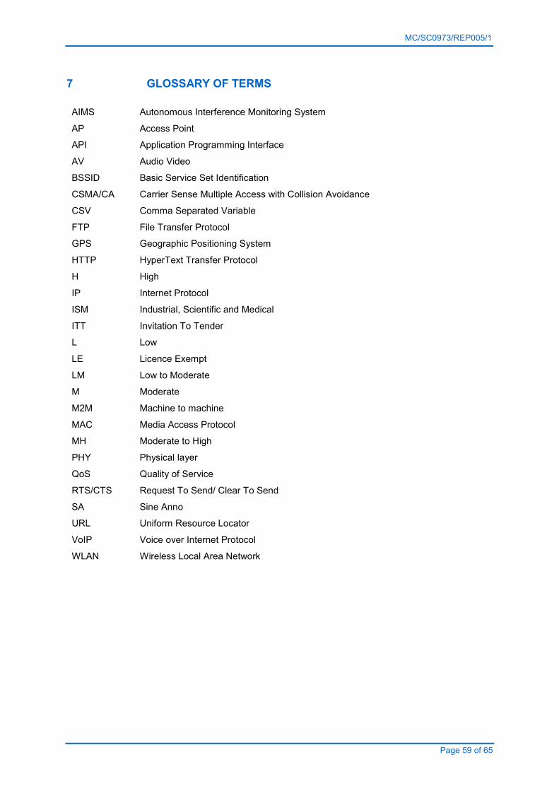
MC/SC0973/REP005/1
Page 59 of 65
7 GLOSSARY OF TERMS
AIMS Autonomous Interference Monitoring System
AP Access Point
API Application Programming Interface
AV Audio Video
BSSID Basic Service Set Identification
CSMA/CA Carrier Sense Multiple Access with Collision Avoidance
CSV Comma Separated Variable
FTP File Transfer Protocol
GPS Geographic Positioning System
HTTP HyperText Transfer Protocol
H High
IP Internet Protocol
ISM Industrial, Scientific and Medical
ITT Invitation To Tender
L Low
LE Licence Exempt
LM Low to Moderate
M Moderate
M2M Machine to machine
MAC Media Access Protocol
MH Moderate to High
PHY Physical layer
QoS Quality of Service
RTS/CTS Request To Send/ Clear To Send
SA Sine Anno
URL Uniform Resource Locator
VoIP Voice over Internet Protocol
WLAN Wireless Local Area Network

MC/SC0973/REP005/1
Page 60 of 65
8 DEFINITIONS
Congestion A network link is congested when the offered load on the link reaches a value close to the capacity of the link (Jardosh et al, 2005b)
Degradation A network link is degraded when its capacity for carrying traffic has been reduced for whatever reason.
Higher layer utilisation The percentage of time in the layers above the MAC for which there are bits present.
Interference Noise or other external signals coming from other devices, such as microwave ovens and other wireless network devices that will result in delay to the user either by blocking transmissions from clients on the WLAN or by causing bit errors to occur in data being sent (Vines, 2002, pp. 234-235)
Link layer utilisation The percentage of time in the MAC for which there are bits present.
MAC stress The percentage of time in which the MAC is not capable of transferring data. Note that we currently estimate this parameter using the percentage of frames that have their retry flags set, but recognise that a better estimator is required and have included this in our recommendations for further work.
Network density The number of unique BSSIDs observed in the measurement interval.
Occupancy In this report the term occupancy is used as a synonym for physical layer utilisation. It is percentage of time in which the received signal strength exceeds a threshold (see section 4.3).
Offered load The total number of bits presented for transmission over a wireless network per second.
Physical layer utilisation In this report also called occupancy, it is the percentage time for which the received signal power is above the measurement threshold (see section 4.3)
Throughput The throughput is the total number of bits transmitted over a wireless channel per second (Jardosh et al, 2005b). As not all the offered load may be carried successfully by the network, throughput can be less than offered load.
In this study we use the number of bits in the MAC layer for the purposes of measuring throughput. We have used units of MB/hr and GB/hr to avoid the issues of comparison with headline data rates. Such comparisons are not helpful when considering the amount of data that can be transferred by a spectrum band.
Utilisation A generic term indicating the proportion of time for which a condition exists within a defined frequency band. Three types of utilisation are considered in this report: physical layer utilisation (or occupancy), link layer utilisation and higher layer utilisation.
MC/SC0973/REP005/1
Page 61 of 65
9 REFERENCES
Aguayo, D., Bicket, J., Biswas, S., Judd, G. and Morris, R. (2004) Link-level measurements from an
802.11b mesh network [online], http://sing.stanford.edu/cs303-sp10/papers/p442-aguayo.pdf
(Accessed 18 September 2012).
Allan, D.W. (1987) Time and frequency (time-domain) characterization, estimation, and prediction of
precision clocks and oscillators, IEEE Transactions on Ultrasonics, Ferroelectrics and Frequency
Control. Vol. UFFC-34, No. 6.
Bianchi, G. (1998) IEEE 802.11 – Saturation throughput analysis [online], IEEE Communications
Letters, vol. 2, no. 12, pp.318-320, http://www.icg.isy.liu.se/courses/tsin01/material/Bianchi1998.pdf
(Accessed 10 September 2012).
Cardoso, L.S., Kobayashi, M., Ryan, Ø. and Debbah, M. (2008) Vandermonde frequency division
multiplexing for cognitive radio [online], folk.uio.no/oyvindry/CognitiveVFDMver5.pdf.
Chernicoff, D. (2011) Too many mobile wireless hotspots makes for a bad day [online],
http://www.zdnet.com/blog/datacenter/too-many-mobile-wireless-hotspots-makes-for-a-bad-day/994
(Accessed 22 March 2013).
Cisco (2004) Channel deployment issues for 2.4-GHz 802.11 WLANs [online],
http://www.cisco.com/en/US/docs/wireless/technology/channel/deployment/guide/Channel.html
(Accessed 14 February 2013).
Coleman, D. (2012) Wi-Fi back to basics – 2.4 GHz channel planning [online],
http://blogs.aerohive.com/blog/the-wireless-lan-training-blog/wifi-back-to-basics-24-ghz-channel-
planning (Accessed 25 March 2013).
Cunningham, M. and Mitchell, S. (2007) A study into licence exempt application specific bands for
Ofcom [online], Red-M final report. GCD-CSG 1503 version 1.4,
http://stakeholders.ofcom.org.uk/binaries/research/technology-research/leasb1.pdf (Accessed 11
Janaury 2013).
Day, S. and Merricks, N.P. (2003) AY4434 – 2.4 GHz Monitoring Exercise, MASS
MC/SC0390/REP010/1.
Dimatteo, S., Hui, P. Han, B. and Li, V.O.K. (2011) Cellular traffic offloading through WiFi networks
[online], http://www.deutsche-telekom-laboratories.de/~panhui/publications/mass11offload.pdf
(Accessed 19 February 2013).
Duda, A. (2008) Understanding the performance of 802.11 networks [online], http://www-r2.u-
strasbg.fr/~pansiot/enseignement/Master%2520Recherche/PIMRC08-80211-DudaA.pdf (Accessed 17
January 2013).
EBU (2011) The future of terrestrial broadcasting [online],
https://tech.ebu.ch/docs/techreports/tr013.pdf#page28.
Fei, H. and Yu, B. (2008) A multiscale analysis and modelling of wireless traffic, IEEE International
Symposium on Information Science and Engineering, pp. 209-212.
Gember, A., Anand, A. and Akella, A. (2011) A comparative study of handheld and non-handheld
traffic in campus WiFi networks [online], http://www.agember.com/docs/gember2011pam.pdf
(Accessed 14 September 2012).
Hansell, P., Kirtay, S., Inglis, I., Pahl, J. and Munday, S. (2004) Evaluating spectrum percentage
occupancy in licence-exempt allocations [online], Aegis Spectrum Engineering and Transfinite
MC/SC0973/REP005/1
Page 62 of 65
Systems final report. 1606/LEM/R/3, http://www.aegis-
systems.co.uk/download/1606/perc_ocp_lisc.pdf (Accessed 11 January 2013).
Han-Lin, S., Yue-Hui, J., Yi-Dong, C. and Shi-Duan, C. (2009) Network traffic prediction by a wavelet-
based combined model, Chinese Physics B, Vol. 18, No. 11, pp. 4760-68.
Horowitz, M. (2012) Wi-Fi in an apartment building [online], http://blogs.computerworld.com/wireless-
networking/20616/wi-fi-apartment-building (Accessed 21 March 2013).
Indepen, Aegis and Ovum (2006) The economic value of licence exempt spectrum [online],
http://www.aegis-systems.co.uk/download/1818/value.pdf (Accessed 11 January 2013).
Islam, M.H., Koh, C.L., Oh, S.W., Qing, X., Lai, Y.Y., Wang, C., Liang, Y-C., Toh, B.E., Chin, F. Tan,
G.L. and Toh, W. (2008) Spectrum survey in Singapore: Occupancy measurements and analyses
[online],
http://www.pwtc.eee.ntu.edu.sg/News/Documents/Spectrum%20survey%20in%20Singapore_%20Occ
upancy%20measurements%20and%20analyses.pdf (Accessed 5 February 2013).
Jardosh, A.P., Ramachandran, K.N., Almeroth, K.C. and Belding-Royer, E.M. (2005a) Understanding
link-layer behavior in highly congested IEEE 802.11b wireless networks, SIGCOMM ‘05 Workshops,
22-26 August 2005, Philadelphia, USA.
Jardosh, A.P., Ramachandran, K.N., Almeroth, K.C. and Belding-Royer, E.M. (2005b) Understanding
congestion in IEEE 802.11b wireless networks, Proceedings of the Internet Measurement Conference
2005, Berkeley, California, USA, pp. 279-292.
Kashyap, A., Paul, U. and Das, S.R. (2010) Deconstructing interference relations in WiFi networks
[online], http://www.wings.cs.sunysb.edu/~upaul/paper/Secon_paper.pdf (Accessed 14 September
2012).
Kirkman ATDI Ltd. (2007) Red-M Spectrum efficiency scheme project. Interference modelling report
[online] ATDI, http://stakeholders.ofcom.org.uk/binaries/research/technology-research/leasb2.pdf
(Accessed 11 January 2013).
Lee, K., Rhee, I., Lee, J., Chong, S. and Yi, Y. (2010) Mobile data offloading: How much can WiFi
deliver? [online] http://lanada.kaist.ac.kr/pubs/WiFi_Offloading_2010conext.pdf, (Accessed 14
September 2012).
López-Benítez, M., Umbert, A. and Casadevall, F. (2009) Evaluation of spectrum occupancy in Spain
for cognitive radio applications [online],
http://www.lopezbenitez.es/int_conferences/VTC_2009_Spring.pdf (Access 5 February 2013).
Ofcom (2012) Determining the Utilisation of Key Licence Exempt Bands and the Effects on Wireless
LAN Performance, MC No.: MC/137.
Maraslis, K., Chatzimisios, P. and Boucouvalas, A. (2012) IEEE 802.11aa: Improvements on video
transmission over wireless LANs [online], aetos.it.teithe.gr/~peris/research/ICC_2012_802.11aa.pdf.
McHenry, M. and McCloskey, D. (2006) Multi-band, multi-location spectrum occupancy measurements
[online], http://www.its.bldrdoc.gov/isart/art06/slides06/mch_m/mch_m_slides.pdf (Accessed 5
February 2013).
Merricks, N.P. and Hansell, P. (2007) Autonomous Interference Monitoring System. Licence Exempt
Spectrum Measurement Study. Volume 1 – Summary Report. MASS MC/SC0585/REP010/2.
Metageek (2012) Optimizing wireless networks [online], http://www.metageek.net/wp-
content/uploads/2012/08/MetaGeek_OptimizingWirelessNetworks_2012.pdf (Accessed 14 February
2013).

MC/SC0973/REP005/1
Page 63 of 65
Raghavendra, R., Pahye, J., Mohajan, R. and Belding, E. (2009) Wi-Fi networks are underutilized
[online] http://research.microsoft.com/pubs/101852/wifi-networks-are-underutilized.pdf (Accessed 13
September 2012).
Ray, B. (2009) Ofcom works out why Wi-Fi doesn’t work [online], The Register,
http://www.theregister.co.uk/2009/05/10/ofcom_mass_wi_fi/ (Accessed 14 February 2012).
Roberson, D.A., Hood, C.S., LoCicero, J.L. and MacDonald, J.T (2006) Spectral occupancy and
interference studies in support of cognitive radio technology development [online],
http://ntrg.cs.tcd.ie/en/TCD_VT_Course_Cognitive_Radios_and_Networks/Week%203/Readings_and
_Discussion_Questions/Spectral%20Occupancy%20and%20Interference%20Studies.pdf (Accessed 5
February 2013).
Rodrig, M., Reis, C., Mahajan, R., Wetherall, D. and Zahorjan, J. (2005) Measurement-based
characterization of 802.11 in a hotspot setting, SIGCOMM’05, 22-26 August 2005, Philadelphia, PA,
USA.
Scientific Generics (2006) Understanding the scope for a power increase for wireless broadband
access at 2.4 GHz & 5.x GHz. Final report [online], Ofcom reference C31400/013/1510,
http://stakeholders.ofcom.org.uk/binaries/research/technology-research/005_final-report-1-6.pdf
(Accessed 11 January 2013).
Sheth, A., Doerr, C., Grunwald, D., Han, R. and Sicker, D. (2006) MOJO: A distributed physical layer
anomaly detection system for 802.11 WLANs [online],
http://static.usenix.org/events/mobisys06/full_papers/p191-sheth.pdf (Accessed 18 September 2012).
Simek, M., Fuchs, M., Mraz, L., Moravek, P. and Botta, M. (20011) Measurement of LowPAN network
coexistence with home microwave appliances in laboratory and home environments, 2011
International Conference on Broadband and Wireless Computing, Communication and Applications
(BWCCA), 26-28 October 2011, Barcelona, Catalonia, Spain.
Sommers, J. and Barford, P. (2012) Comparing metro-area cellular and WiFi performance [online],
SIGMETRICS’12 11-15 June 2012, London, England, http://pages.cs.wisc.edu/~pb/sigm12_paper.pdf
(Accessed 10 September 2012).
Thompson, B. (2009) Can’t connect, won’t connect [online],
http://news.bbc.co.uk/1/hi/technology/8044266.stm (Accessed 10 February 2012).
Tian, X., Wu, J. and Ji, C. (2002) A unified framework for understanding network traffic using
independent wavelet models, IEEE Infocom 2002, pp. 446-454.
Valenta, V., Fedra, Z., Maršálek, R., Baudoin, G. and Villegas, M. (2009) Towards Cognitive Radio
Networks: Spectrum Utilization Measurements in Suburb Environment [online],
http://hal.inria.fr/docs/00/44/69/58/PDF/RWS_SANDIEGO_VALENTA.pdf (Accessed 5 February
2013).
van Bloem, J-W and Schiphorst, R. (2011) Measuring the service level in the 2.4 GHz ISM band
[online], University of Twente, report number SAS2011-017,
http://eprints.eemcs.utwente.nl/20915/01/report.pdf (Accessed 10 January 2013).
Vines, R.D. (2002) Wireless security essentials, Indianapolis, Indiana, Wiley Publishing Inc.
Wagstaff, A.J. and Merricks, N.P. (2006) Autonomous Interference Monitoring System. Final Report.
MASS MC/SC0526/REP020/2.
Wagstaff, A.J. and Merricks, N.P. (2007) Autonomous Interference Monitoring System. Phase 2. Final
Report. MASS MC/SC0585/REP016/1.

MC/SC0973/REP005/1
Page 64 of 65
Wagstaff, A.J. (2009) Estimating the Utilisation of Key Licence-Exempt Spectrum Bands. Final Report.
MASS MC/SC0710/REP003/3.
Wagstaff, A.J. (2012) Proposal for a study to determine the utilisation of key Licence Exempt bands
and the effects on WLAN performance. MASS MC/SB0973/PRO001/2.
Williamson, B., Punton, T. and Hansell, P. (2013) Future proofing WiFi – the case for more spectrum
[online], http://www.plumconsulting.co.uk/pdfs/Plum_Jan2013_Future_proofing_Wi-Fi.pdf (Accessed
19 February 2013).
Wong, M. and Clement, A. (2006) Sharing wireless internet in urban neighbourhoods [online],
http://www.cwirp.org/files/wong_C&T.pdf (Accessed 19 February 2013).
Zhang, X. and Shin, K.G. (2013) Gap Sense: Lightweight coordination of heterogenous wireless
devices [online], kabru.eecs.umich.edu/papers/publications/2013/xyzhang_kgshin_infocom13.pdf.
MC/SC0973/REP005/1
Page 65 of 65
10 BIBLIOGRAPHY
Aegis (2011) In-home propagation. Final report, Aegis Systems Ltd., 2216/IHP/R/1/1.4,
http://stakeholders.ofcom.org.uk/binaries/research/technology-research/2011/IHP_Final_Report.pdf
(Accessed 11 January 2013).
Afanasyev, M., Chen, T., Voelker, G.M. and Snoeren, A.C. (2008) Analysis of a mixed-use urban WiFi
network: When metropolitan becomes Neapolitan [online],
http://cseweb.ucsd.edu/~voelker/pubs/google-imc08.pdf (Accessed 19 February 2013).
Angrisani, L., Kyriakopoulos, K., Napolitano, A., Parish, D.J., Vadursi, M. and Whittow, W. (2010) ‘An
experimental analysis of the effects of noise on Wi-Fi video streaming’, 2010 IEEE Instrumentation
and Measurement Technology Conference, 3-6 May 2010, Nales, Italy.
Bhadauria, A. (2007) WiFiNetMon: Interference measurement in long distance WiFi mesh networks.
MSc thesis, Indian Institute of Technology.
Brik, V., Rayanchu, S., Saha, S., Sen, S., Shrivastava, V. and Banerjee, S. (2008) A measurement
study of a commercial-grade urban WiFi mesh [online] http://pages.cs.wisc.edu/~shravan/mcb.pdf
(Accessed 14 September 2012).
Chebrolu, K., Raman, B. and Sen, S. (2006) Long-distance 802.11b links: Performance
measurements and experience, MobiCom ’06, 23-26 September 2006, Los Angeles, California, USA.
Haider, F., Hepsaydir, E. and Binucci, N. (SA) Performance analysis of a live mobile broadband –
HSDPA network [online], http://home.eps.hw.ac.uk/~fsh12/HSDPA_paper.pdf.
Henty, B. (2001) Throughput measurements and empirical prediction models for IEEE 802.11b
wireless LAN (WLAN) installations [online], Phd Thesis, Virginia Polytechnic Institute and State
University, http://scholar.lib.vt.edu/theses/available/etd-08142001-172523/unrestricted/hentythesis.pdf
(Accessed 18 September 2012).
Mahajan, R., Rodrig, M., Wetherall, D. and Zahorjan, J. (2006) Analyzing the MAC-level behavior of
wireless networks in the wild, Proceedings SIGCOMM ’06, 11-15 September 2006, Pisa, Italy.
Mahanti, A., Williamson, C. and Arlitt, M. (2007) ‘Remote analysis of a distributed WLAN using passive
wireless-side measurement’, Performance Evaluation, 64(2007) pp. 909-932.
Najafzadeh, E., George, D. and Green, P. (2012) LabVIEW-based spectrum occupancy
measurements in the 2.4 GHz ISM band using National Instruments USRP [online], http://www.arsr-
swicom.org.uk/papersandposters/2012/arsr-papers/ENajafzaden-Spectrum-Occupancy.pdf.
Rajagopalan, G. (2008) 802.11n client throughput performance [online], http://bradreese.com/aruba-
test.pdf (Accessed 31 October 2012).
Sen, S., Yoon, J., Hare, J., Ormont, J. and Banerjee, S. (2011) Can they hear me now?: A case for a
client-assisted approach to monitoring wide-area wireless networks [online], IMC ’11, 2-4 November
2011, Berlin, Germany, http://pages.cs.wisc.edu/~suman/pubs/wiscape.pdf (Accessed 15 January
2013).
Wikipedia (2013) IEEE 802.11 [online], http://en.wikipedia.org/wiki/IEEE_802.11 (Accessed 17
January 2013).
Yijie, C. (2008) Simulation study of HTTP traffic in WLAN [online],
http://www.paper.edu.cn/download/downPaper/200811-608 (Accessed 15 January 2013).