, 20110548371 2013 Phil. Trans. R. Soc. A Mukund Thattai of genetic networksUsing topology to tame the complex biochemistry  

Supplementary data

rsta.2011.0548.DC1.html http://rsta.royalsocietypublishing.org/content/suppl/2013/01/03/

"Audio Supplement"

References48.full.html#ref-list-1http://rsta.royalsocietypublishing.org/content/371/1984/201105

This article cites 55 articles, 14 of which can be accessed free

This article is free to access

Subject collections

(56 articles)biophysics   � collectionsArticles on similar topics can be found in the following

Email alerting service herein the box at the top right-hand corner of the article or click Receive free email alerts when new articles cite this article - sign up

http://rsta.royalsocietypublishing.org/subscriptions go to: Phil. Trans. R. Soc. ATo subscribe to

on January 14, 2013rsta.royalsocietypublishing.orgDownloaded from

rsta.royalsocietypublishing.org

ReviewCite this article: Thattai M. 2013 Usingtopology to tame the complex biochemistry ofgenetic networks. Phil Trans R Soc A 371:20110548.http://dx.doi.org/10.1098/rsta.2011.0548

One contribution of 17 to a Discussion MeetingIssue ‘Signal processing and inference for thephysical sciences’.

Subject Areas:biophysics

Keywords:synthetic biology, feedback loops,Boolean threshold models

Author for correspondence:Mukund Thattaie-mail: thattai@ncbs.res.in

Using topology to tame thecomplex biochemistry ofgenetic networksMukund Thattai

National Centre for Biological Sciences, Tata Institute ofFundamental Research, UAS/GKVK Campus, Bellary Road,Bangalore 560065, India

Living cells are controlled by networks of interactinggenes, proteins and biochemicals. Cells use theemergent collective dynamics of these networks toprobe their surroundings, perform computations andgenerate appropriate responses. Here, we considergenetic networks, interacting sets of genes thatregulate one another’s expression. It is possible toinfer the interaction topology of genetic networksfrom high-throughput experimental measurements.However, such experiments rarely provide informationon the detailed nature of each interaction. We showthat topological approaches provide powerful meansof dealing with the missing biochemical data. Wefirst discuss the biochemical basis of gene regulation,and describe how genes can be connected intonetworks. We then show that, given weak constraintson the underlying biochemistry, topology alonedetermines the emergent properties of certain simplenetworks. Finally, we apply these approaches tothe realistic example of quorum-sensing networks:chemical communication systems that coordinate theresponses of bacterial populations.

1. IntroductionGenes are physically embodied as a string of nucleotidebases (ATGGCCCTG. . . ) on a self-replicating DNAmolecule, contained within the cytoplasm of a prokaryoteor the nucleus of a eukaryote. Genes encode proteins,which in turn carry out the processes required for themaintenance of cellular life. During the process of geneexpression, the genetic information is first transcribedor copied onto a short-lived messenger RNA (mRNA)

c© 2012 The Authors. Published by the Royal Society under the terms of theCreative Commons Attribution License http://creativecommons.org/licenses/by/3.0/, which permits unrestricted use, provided the original author andsource are credited.

on January 14, 2013rsta.royalsocietypublishing.orgDownloaded from

2

rsta.royalsocietypublishing.orgPhilTransRSocA371:20110548

......................................................

proteinRNADNA

proteinRNADNA

(a)

(b)

Figure 1. (a) The central dogma of molecular biology. (b) A more accurate representation of the central dogma, with filledarrows representing potential regulatory interactions.

molecule. This mRNA is then translated repeatedly into a protein, as specified by the geneticcode: a set of three consecutive nucleotides of mRNA uniquely specifies one of twenty possibleamino acids, a series of which are strung together to form the protein (the short sequence above,for example, encodes the first three amino acids of the human insulin protein).

This basic description, the ‘central dogma of molecular biology’ (figure 1a), is not the entirestory however. Every cell in the human body carries the same complement of genes, yet a heartcell and a brain cell are made up of very different proteins. Even in a single-celled organism suchas a bacterium, different proteins are expressed at different times. The bacterium Escherichia coliis able to assemble flagella when it needs to swim, and pili when it needs to anchor itself to asurface; it will produce a metabolic enzyme only when its substrate is present, and synthesizeDNA repair proteins only when subject to shock. In short, genes can be turned on and off.

This simple but powerful idea was first proposed by Jacques Monod in the 1940s [1], and theframework he constructed remains essentially unchallenged to this day. The expression of genesis a tightly regulated process [2, ch. 7]. Central to this process is a control element known as apromoter—a short stretch of DNA that precedes every gene. The promoter contains a bindingsite for the RNA polymerase, the protein complex responsible for transcription. Correspondingly,mRNAs contain binding sites for ribosomes, the protein complexes responsible for translation.The rate of transcription at a promoter can be increased or decreased by proteins known astranscription factors that bind DNA in the vicinity of the promoter. In prokaryotes, transcriptionfactors typically bind within a few tens of bases of the promoter, whereas in eukaryotes, long-distance interactions between transcription factors and the RNA polymerase can extend overmegabases. Eukaryotes also have additional ‘epigenetic’ mechanisms to regulate transcription,via covalent modifications of the histone proteins on which DNA is wrapped, or modifications ofthe DNA itself. Once an mRNA molecule is transcribed, its rate of translation can be regulated byproteins that influence the capacity of ribosomes to bind ribosome binding sites, or by proteincomplexes that degrade specific mRNAs. Additionally, it has become clear that a significantfraction of transcribed RNAs do not encode proteins; rather, many of these non-coding RNAscan themselves regulate the translation of mRNAs to proteins, via the sophisticated machinery ofRNA interference [3]. Taking all these effects into account, the central dogma must be modifiedwith a few additional arrows (figure 1b).

These new arrows are loaded with implications: they permit us to assemble complex networksof transcriptional and regulatory interactions. Gene A can activate gene B and gene C, butrepress gene D, and so on. There is a compelling case to be made for the existence of suchnetworks in living cells. Consider that a bacterial genome contains about 4000 genes, whereasthe human genome contains about 25 000 genes—a surprisingly modest difference at first glance,given that the human body is made up of more than 200 cell types, not to mention higherdegrees of organization required to specify a complex tissue such as the brain. A deeper analysissuggests that gene number is not the correct measure of complexity: the properties of a cellare specified by the proteins contained within it; the range of possible cell types is thereforedetermined by the range of possible combinations of expressed genes, and grows exponentiallywith gene number. How are all such combinations to be accessed, however? We know that distinct

on January 14, 2013rsta.royalsocietypublishing.orgDownloaded from

3

rsta.royalsocietypublishing.orgPhilTransRSocA371:20110548

......................................................

external signals can drive cells to differentiate into distinct types. However, such signals do notdirectly interact with individual genes, turning them on or off. Once the differentiation processis triggered, various combinations of gene expression must arise through the intrinsic behaviourof the genes themselves. That is, there must be a network of genetic interactions which, basedon very few external regulatory cues, is able to produce the correct expression patterns. Themanifest complexity of cellular behaviour strongly implies the existence of complex regulatorynetworks within.

In recent times, we have been able to resolve network architecture in unprecedented detailusing high-throughput biochemical experiments, or by inference from gene expression and geneknockout data [4–8]. For certain well-studied organisms such as Escherichia coli and the yeastSaccharomyces cerevisiae, there is a growing body of detailed information regarding transcriptionaland regulatory interactions [9–12]. When these data are combined, what emerges is a picture ofhighly structured networks with rich topologies [13], containing recurring motifs or patterns [14,15], very different from randomly connected sets of genes. Just as individual proteins have beenselected for function, entire networks seem to be similarly selected. So here is what one might callthe central idea of network biology: that the complex behaviour of living cells must be understoodas emerging not just from the properties of individual genes, but from the manner in which theyare connected.

2. The control of gene expressionFor the purposes of this exposition, we focus on prokaryotic gene regulation via promoters.A promoter is a loosely defined object. We can take it to signify a stretch of DNA, upstream ofevery gene, which controls whether that gene is expressed or not. The properties of a promoter,like those of a gene, are determined by its DNA sequence. A survey of bacterial promoters revealsa conserved pattern of nucleotides, all variations of a particular consensus sequence. The mostconserved regions are two short stretches situated −35 and −10 nucleotides from the site atwhich transcription begins [2, ch. 7]. These regions are thought to provide the binding site that isspecifically recognized by the RNA polymerase protein (figure 2a).

There are in fact numerous proteins that, like the polymerase, are able to recognize and bindspecific nucleotide sequences. Their binding sites are typically between six and 20 base pairs inlength. Binding is mediated by physical interactions between residues on the protein and on theDNA molecule. Given the structure of a protein we should, in principle, be able to calculate itsinteraction energy with a particular DNA sequence. The result of such a calculation would bethe ‘DNA-binding code’. The search for such a code is an active area of research [16–18], butfor the time being we can rely on experimental measurements of binding affinities [7,8]. Variousclasses of DNA-binding proteins are known, grouped according to the structure of their DNArecognition domains. These proteins are often modular, having one domain that binds DNA,and another that is responsible for regulatory interactions. Once bound to DNA, a protein canrecruit other proteins to its vicinity, or can prevent them from binding. In particular, a DNA-binding protein can interact with and influence the binding and transcriptional activity of theRNA polymerase. Such molecules are known as gene regulatory proteins or transcription factors.They can be classified as activators (which increase the rate of polymerase binding) or repressors(which prevent the polymerase from binding or block it from transcribing). A given protein mightactivate or repress transcription depending on the relative position of its binding sequence to thatof the RNA polymerase.

The activity of a transcription factor can itself be modulated by the binding of small moleculesor by covalent modification [2, chs 7 and 15]. For example, the E. coli lac repressor, which blockstranscription at the lac operon, contains binding sites for a sugar called allolactose; when therepressor is bound to allolactose, it is unable to bind DNA, and therefore unable to represstranscription. This type of modulation is a key mechanism by which external signals can regulategene expression. Many small molecules in the environment can diffuse across the bacterialcell membrane to directly influence intracellular transcription factors. Other types of signalling

on January 14, 2013rsta.royalsocietypublishing.orgDownloaded from

4

rsta.royalsocietypublishing.orgPhilTransRSocA371:20110548

......................................................

mRNA

TF RNAP

–35TF binding site

D + X DXK 0

eX DX

D

promoter gene–10

1.0

0.8

0.6

0.4

0.2

0 0.5 1.0 1.5 2.0

n = 1n = 2

n = 6

℘ (

D)

[X ]

(a)

(b)

(c)

Figure 2. Protein–DNA interactions. (a) Genes are DNA regions that are transcribed into mRNA, and eventually translatedinto proteins. Promoters are DNA regions upstream of genes where the RNA polymerase molecule (RNAP) binds and initiatestranscription. Transcription factors (TFs) can bind near promoters and interact with the polymerase, exerting regulatory control.(b) The binding of a single protein is shown in the reaction-kinetic (left) and energetic (right) representations. (c) Free DNAas a function of protein levels. The graphs are of Hill functions, showing hyperbolic (n= 1) as well as sigmoidal (n= 2,n= 6) binding curves. Higher Hill coefficients produce more threshold-like functions. The half-saturation concentration is onein each case.

molecules can bind the extracellular domains of transmembrane proteins known as receptors;this causes a conformational change in the receptor’s intracellular domain, which can drive thesubsequent activation or inhibition of transcription factors by phosphorylation. For example, alarge number of bacterial ‘two-component systems’, consisting of a membrane-bound sensor andintracellular transcriptional regulator, operate on this principle. As we show later, these types ofregulatory inputs influence intracellular network dynamics, allowing cells to sense environmentalconditions and respond appropriately.

We can calculate the expression level at a particular promoter from a biophysical model thatincorporates the microscopic details just mentioned, using an approach pioneered by Shea &Ackers [19] in their study of the OR control system of bacteriophage λ. To do this, we first listall possible promoter configurations (the combinations in which the promoter binds variousregulatory proteins or the RNA polymerase); and we specify the relative free energies of each ofthese states. Once this information is given, there is a well-defined thermodynamic prescriptionfor calculating system properties. Consider a DNA region D that can bind a set of proteins Xi(i = 1, . . . , n), each with multiplicity mi. Let the cytoplasmic protein concentrations be [Xi]. Thisbinding event can be represented as

D + m1X1 + m2X2 + · · · + mnXnk+�k−

D · X1m1 · X2m2 · · · Xnmn . (2.1)

For simplicity in the discussion that follows, this representation clubs together what are infact several independent binding events, and includes effective rate constants k+ and k− for

on January 14, 2013rsta.royalsocietypublishing.orgDownloaded from

5

rsta.royalsocietypublishing.orgPhilTransRSocA371:20110548

......................................................

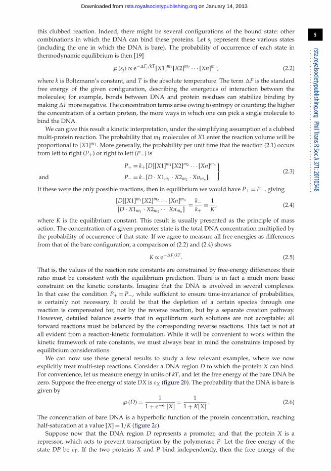
this clubbed reaction. Indeed, there might be several configurations of the bound state: othercombinations in which the DNA can bind these proteins. Let sj represent these various states(including the one in which the DNA is bare). The probability of occurrence of each state inthermodynamic equilibrium is then [19]

℘(sj) ∝ e−�Fj/kT[X1]m1 [X2]m2 · · · [Xn]mn , (2.2)

where k is Boltzmann’s constant, and T is the absolute temperature. The term �F is the standardfree energy of the given configuration, describing the energetics of interaction between themolecules; for example, bonds between DNA and protein residues can stabilize binding bymaking �F more negative. The concentration terms arise owing to entropy or counting: the higherthe concentration of a certain protein, the more ways in which one can pick a single molecule tobind the DNA.

We can give this result a kinetic interpretation, under the simplifying assumption of a clubbedmulti-protein reaction. The probability that m1 molecules of X1 enter the reaction volume will beproportional to [X1]m1 . More generally, the probability per unit time that the reaction (2.1) occursfrom left to right (P+) or right to left (P−) is

P+ = k+[D][X1]m1 [X2]m2 · · · [Xn]mn

and P− = k−[D · X1m1 · X2m2 · Xnmn ].

}(2.3)

If these were the only possible reactions, then in equilibrium we would have P+ = P−, giving

[D][X1]m1 [X2]m2 · · · [Xn]mn

[D · X1m1 · X2m2 · · · Xnmn ]= k−

k+≡ 1

K, (2.4)

where K is the equilibrium constant. This result is usually presented as the principle of massaction. The concentration of a given promoter state is the total DNA concentration multiplied bythe probability of occurrence of that state. If we agree to measure all free energies as differencesfrom that of the bare configuration, a comparison of (2.2) and (2.4) shows

K ∝ e−�F/kT . (2.5)

That is, the values of the reaction rate constants are constrained by free-energy differences: theirratio must be consistent with the equilibrium prediction. There is in fact a much more basicconstraint on the kinetic constants. Imagine that the DNA is involved in several complexes.In that case the condition P+ = P−, while sufficient to ensure time-invariance of probabilities,is certainly not necessary. It could be that the depletion of a certain species through onereaction is compensated for, not by the reverse reaction, but by a separate creation pathway.However, detailed balance asserts that in equilibrium such solutions are not acceptable: allforward reactions must be balanced by the corresponding reverse reactions. This fact is not atall evident from a reaction-kinetic formulation. While it will be convenient to work within thekinetic framework of rate constants, we must always bear in mind the constraints imposed byequilibrium considerations.

We can now use these general results to study a few relevant examples, where we nowexplicitly treat multi-step reactions. Consider a DNA region D to which the protein X can bind.For convenience, let us measure energy in units of kT, and let the free energy of the bare DNA bezero. Suppose the free energy of state DX is εX (figure 2b). The probability that the DNA is bare isgiven by

℘(D) = 11 + e−εx [X]

= 11 + K[X]

. (2.6)

The concentration of bare DNA is a hyperbolic function of the protein concentration, reachinghalf-saturation at a value [X] = 1/K (figure 2c).

Suppose now that the DNA region D represents a promoter, and that the protein X is arepressor, which acts to prevent transcription by the polymerase P. Let the free energy of thestate DP be εP. If the two proteins X and P bind independently, then the free energy of the

on January 14, 2013rsta.royalsocietypublishing.orgDownloaded from

6

rsta.royalsocietypublishing.orgPhilTransRSocA371:20110548

......................................................

X

X

P

DX

D DXP

DPP

K1

K3K4

K2

X

X

XDXA

D DXAXB

DXBX

K1

K3K4

K2

0 DeX

eP

eP + eX

DX

DPDXP

0 DeA

eB

eAB =eA + eB + DeAB

DXA

DXB

DXAXB

(a)

(b)

Figure 3. Transcriptional regulation by DNA-binding proteins. (a) Independent binding of a repressor (X) and the polymerase(P). The free energy of the doubly bound state is the sumof the individual binding energies. (b) Cooperative binding. The bindingof a single molecule of X increases the likelihood that a second molecule will bind.

doubly bound state DXP will be the sum of the individual binding energies. (If the independent-binding assumption is not valid, the energy of the state DXP must be provided as an additionalparameter.) The energies of the various bound states in this scenario are indicated in figure 3a.The only state from which transcription can proceed is the state DP. Applying the equilibriumprescription, we find that this state occurs with probability

℘(DP) = e−εP [P]1 + e−εP [P] + e−εX [X] + e−εP−εX [P][X]

= e−εP [P]1 + e−εP [P]

11 + e−εX [X]

, (2.7)

where we have explicitly factorized the expression. This factorization is possible precisely becausethe proteins X and P bind independently, so the probability that state DP occurs is the probabilitythat P is bound multiplied by the probability that X is not bound (the latter being given by (2.6)).It is instructive to see how the derivation might proceed from the kinetic framework. Applyingdetailed balance, we can find two expressions for the concentration of the doubly bound state,corresponding to the upper and lower binding paths:

[DXP][D][X][P]

= K1K2 = K3K4. (2.8)

The four dissociation constants cannot, therefore, be independently specified. (Note also that, bythe independent binding property, K1 = K4 = e−εX and K2 = K3 = e−εP .)

In many instances, transcription factors bind to multiple sites. Suppose the promoter inquestion contains two sites, A and B, to which X can bind in any order (figure 3b). Let the freeenergies of the two singly bound states be εA and εB, and that of the doubly bound state beεAB = εA + εB + �εAB. These assumptions correspond to the most general situation, of which thefollowing are special cases: if the two sites are identical, then εA = εB; if X binds independentlyto these sites, then �εAB = 0. The energy term �εAB corresponds to some interaction between thetwo bound copies of X. If the binding of a single molecule makes it more favourable for another tobind, a condition referred to as positive cooperativity, then �εAB < 0. Conversely, in a situation ofnegative cooperativity, �εAB > 0, and the binding of one molecule interferes with the ability of the

on January 14, 2013rsta.royalsocietypublishing.orgDownloaded from

7

rsta.royalsocietypublishing.orgPhilTransRSocA371:20110548

......................................................

other to bind. Positive cooperativity is the norm among transcription factors that act multiply. Letus see what effect this will have. Assume, for simplicity, that |εA| ∼ |εB| � |�εAB|. In the kineticframework, this corresponds to K1 � K2, and K3 � K4, with the detailed balance condition againas shown in (2.8). We find

[Dtot][X][DXA]

>[D][X][DXA]

= 1K1

� 1K2

= [DXA][X][DXAXB]

>[DXA][X]

[Dtot], (2.9)

where the inequalities are obtained by noticing that the concentration of any DNA configurationmust be less than that of the total amount of DNA available. This shows that [DXA] � [Dtot],and similarly, [DXB] � [Dtot]: the singly bound configurations form a negligible fraction of thepopulation. No sooner has one molecule of X bound DNA, than the second also binds. Therefore,the probability that the DNA is bare is given by

℘(D) = 11 + e−εAB [X]2 = 1

1 + K1K2[X]2 . (2.10)

The cooperativity of binding gives rise to the quadratic term in the denominator. The bindingcurve is sigmoidal, meaning that it has an inflection point at [X] = 1/K1K2 (figure 2c). In theliterature, as a first approximation, binding probabilities are often parametrized as Hill equations

℘(D) = 11 + ([X]/[X0])n , (2.11)

with n being the Hill coefficient (a measure of cooperativity) and [X0] being the half-saturationconcentration. The hyperbola (2.6) (with n = 1) and the sigmoid (2.10) (with n = 2) can both beparametrized in this way (figure 2c). These parameters, among many others, are required toprovide a detailed biochemical description of any genetic network.

3. Genetic networks

(a) The network equationSingle genes are often regulated by multiple transcription factors that interact with one another.A classic example is the lac operon, which is regulated by both a repressor and an activator [20].In eukaryotes, a single gene could be regulated by dozens of proteins. It is a remarkable fact that,using only thermodynamic constraints of the type we have considered, a promoter can be made toperform a variety of mathematical operations on its regulatory inputs. Specifically, the probabilityof occurrence of the transcriptionally active promoter configuration can be a complicated functionof the concentration of various transcription factors [21–26]. These concentrations can themselveschange over time owing to regulation of the genes encoding the transcription factors. If we wishto understand the behaviour of the system, we must therefore consider the regulatory network asa whole. We now try to arrive at a general mathematical description of such networks.

The rate of protein creation per promoter, α, is a product of the following terms: the probabilitythat the promoter is transcriptionally active, the rate at which transcription proceeds irreversiblyfrom the active state and the number of proteins translated per resulting transcript. Consider acell that contains nP copies of a gene encoding protein Xi. If the protein once created does notdegrade, then the number of protein molecules ni will obey

dni

dt= nPαi. (3.1)

If the cell volume is V, then the protein concentration xi = [Xi] evolves as

dxi

dt= d

dtnP

Vαi − 1

VdVDt

xi, (3.2)

where the negative term arises owing to dilution.

on January 14, 2013rsta.royalsocietypublishing.orgDownloaded from

8

rsta.royalsocietypublishing.orgPhilTransRSocA371:20110548

......................................................

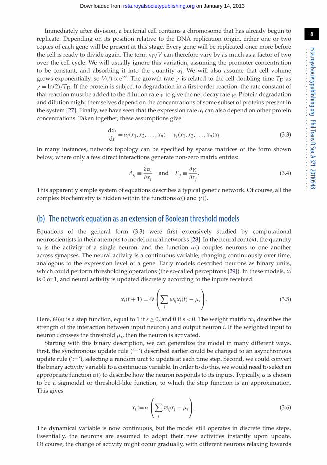
Immediately after division, a bacterial cell contains a chromosome that has already begun toreplicate. Depending on its position relative to the DNA replication origin, either one or twocopies of each gene will be present at this stage. Every gene will be replicated once more beforethe cell is ready to divide again. The term nP/V can therefore vary by as much as a factor of twoover the cell cycle. We will usually ignore this variation, assuming the promoter concentrationto be constant, and absorbing it into the quantity αi. We will also assume that cell volumegrows exponentially, so V(t) ∝ eγ t. The growth rate γ is related to the cell doubling time TD asγ = ln(2)/TD. If the protein is subject to degradation in a first-order reaction, the rate constant ofthat reaction must be added to the dilution rate γ to give the net decay rate γi. Protein degradationand dilution might themselves depend on the concentrations of some subset of proteins present inthe system [27]. Finally, we have seen that the expression rate αi can also depend on other proteinconcentrations. Taken together, these assumptions give

dxi

dt= αi(x1, x2, . . . , xn) − γi(x1, x2, . . . , xn)xi. (3.3)

In many instances, network topology can be specified by sparse matrices of the form shownbelow, where only a few direct interactions generate non-zero matrix entries:

Aij ≡ ∂αi

∂xjand Γij ≡ ∂γi

∂xj. (3.4)

This apparently simple system of equations describes a typical genetic network. Of course, all thecomplex biochemistry is hidden within the functions α() and γ ().

(b) The network equation as an extension of Boolean threshold modelsEquations of the general form (3.3) were first extensively studied by computationalneuroscientists in their attempts to model neural networks [28]. In the neural context, the quantityxi is the activity of a single neuron, and the function α() couples neurons to one anotheracross synapses. The neural activity is a continuous variable, changing continuously over time,analogous to the expression level of a gene. Early models described neurons as binary units,which could perform thresholding operations (the so-called perceptrons [29]). In these models, xiis 0 or 1, and neural activity is updated discretely according to the inputs received:

xi(t + 1) = Θ

⎛⎝∑

j

wijxj(t) − μi

⎞⎠. (3.5)

Here, Θ(s) is a step function, equal to 1 if s ≥ 0, and 0 if s < 0. The weight matrix wij describes thestrength of the interaction between input neuron j and output neuron i. If the weighted input toneuron i crosses the threshold μi, then the neuron is activated.

Starting with this binary description, we can generalize the model in many different ways.First, the synchronous update rule (‘=’) described earlier could be changed to an asynchronousupdate rule (‘:=’), selecting a random unit to update at each time step. Second, we could convertthe binary activity variable to a continuous variable. In order to do this, we would need to select anappropriate function α() to describe how the neuron responds to its inputs. Typically, α is chosento be a sigmoidal or threshold-like function, to which the step function is an approximation.This gives

xi := α

⎛⎝∑

j

wijxj − μi

⎞⎠ . (3.6)

The dynamical variable is now continuous, but the model still operates in discrete time steps.Essentially, the neurons are assumed to adopt their new activities instantly upon update.Of course, the change of activity might occur gradually, with different neurons relaxing towards

on January 14, 2013rsta.royalsocietypublishing.orgDownloaded from

9

rsta.royalsocietypublishing.orgPhilTransRSocA371:20110548

......................................................

the steady state prescribed by (3.6) at different rates γi:

1γi

dxi

dt= α

⎛⎝∑

j

wijxj − μi

⎞⎠− xi. (3.7)

We thus arrive at an equation of the form (3.3). Note, however, that the function α() has avery special form, thresholding a weighted sum of inputs, an approximate phenomenologicaldescription of neural behaviour.

Moving back to genetic systems, how much can we learn by analogy with neural or electronicnetworks? It turns out that, when groups of genes are collected into a network, the resultingarchitecture is markedly different from that of the generic electronic circuit to which it is oftencompared. In the electronic case, large numbers of simple nodes are connected in complexways. In the genetic case, the network is likely to be much more shallow, with each node, apromoter, executing more complex operations [14,21]. A single promoter is capable of respondingin intricate ways to its inputs, and indeed, it is becoming clear that real single neurons mightthemselves be capable of sophisticated computations [30]. The simplicity and uniformity ofelectronic nodes have allowed us to model large electronic circuits very effectively. It is likelythat there will never be an equivalent standard framework for the study of genetic systems—too much depends on the unique characteristics of each gene or protein. This is the biochemicalcomplexity that makes the analysis of genetic networks challenging. Nevertheless, as we discussin §4, topology proves to be a surprisingly useful determinant of network properties.

4. The emergent properties of networks

(a) A biological wish-listImagine that we need to design a regulatory system to orchestrate one of the most intricate ofall known biological processes, the development of a living embryo [31]. What are some of thetasks that need to be carried out, and some of the problems we might encounter along the way?We start with a fertilized egg that has undergone repeated divisions, thus producing a set ofundifferentiated cells. Very soon, this embryo will begin to respond to maternal cues, in the formof spatial gradients of signalling molecules called morphogens, causing cells in different positionsto express different sets of genes. Gene expression levels will need to vary significantly, as wemove across segment boundaries: small changes in the levels of a signalling molecule must beamplified to produce large changes in expression. New transcription factors will be synthesized,triggering a subsequent round of gene expression. Cells will need to respond rapidly to thesechanges. At this stage, small errors in expression patterns must be avoided, as they would lead tolarger and possibly lethal errors in downstream processes. The morphogen signals will eventuallystart to die away; the cells must nevertheless retain some memory of these signals, remainingfirmly committed to their different fates. Developmental processes in different parts of the embryowill need to be synchronized: protein levels will need to oscillate periodically in time. And the listgoes on.

The surprising fact is, each of the tasks on our wish-list can be achieved by small networksof interacting genes (figure 4) [32,33]. In §4b, we survey a few simple networks that areable to generate, in principle, these various biologically desirable outcomes. Over the pastdecade systems such as those discussed here have been explored experimentally by syntheticbiologists [34–36]: negative feedback for noise reduction [37,38]; positive feedback and theflip–flop for bistability [20,39–41]; and hysteretic and ring oscillators [26,42–44].

(b) The dynamics of simple network topologiesAmplification by cooperative activation: consider a gene that encodes a protein Y and is regulatedby an activator X (figure 5a). Cooperative interactions can result in a Hill-type dependence of the

on January 14, 2013rsta.royalsocietypublishing.orgDownloaded from

10

rsta.royalsocietypublishing.orgPhilTransRSocA371:20110548

......................................................

ampli

ficati

on

rapid

equil

ibrati

on

cellu

lar m

emor

y

oscil

lation

s

Figure4. Theemergent properties of networks: amplificationby cooperative activation; rapid equilibration andnoise reductionby negative feedback; memory and bistability by positive feedback and the flip–flop; oscillations by hysteretic and ringoscillators.

gene expression level on the activator concentration. Setting x = [X] and y = [Y],

dydt

= Axn

1 + xn − y, (4.1)

where for notational simplicity, x is measured in units of the half-saturation concentration(compare with (2.11)) and time is measured in units such that the decay rate of y is unity (comparewith (3.3)). The value of the steady-state output, y, can depend sensitively on that of the input, x:

∂ y∂ x

= ∂ ln y∂ ln x

∣∣∣∣x=1

= n2

. (4.2)

At high or low values of x, the value of y is close to either zero or A and is insensitive to changesin the input. However, near the threshold x = 1, a certain fractional change in x is amplified toproduce an n/2 greater fractional change in y: differential input signals will be amplified.

Rapid equilibration and noise reduction by negative feedback: consider what happens whena gene negatively regulates its own expression (figure 5b). Assume that the protein is a repressorthat behaves as shown in (2.6):

dxdt

= A1

1 + x− x ≡ f (x) − g(x). (4.3)

The steady state of the system corresponds to that concentration x at which the rate of creationf (x) and the rate of destruction g(x) balance one another. We see from figure 6a that the negative-feedback system settles into a steady state intermediate between 0 and A (something that cannotbe captured in a pure binary description). If the expression level of the system is transientlyincreased above this steady state, the resulting drop in the creation rate quickly restoresequilibrium. In fact, the auto-repressed system equilibrates more rapidly than an unregulatedsystem with the same steady state, as shown in figure 6a; this has the effect of suppressingstochastic fluctuations [45].

Memory and bistability by positive feedback: we next allow the gene to positively regulate itsown expression (figure 5b). This can be achieved by closing the loop in (4.1):

dxdt

= Axn

1 + xn − x ≡ f (x) − g(x). (4.4)

We see from the binary model that this system can have multiple steady states: a gene that isactive will sustain its own expression, whereas one that is inactive will never become activated(figure 5b). In the continuous model, this would correspond to having multiple values of x at

on January 14, 2013rsta.royalsocietypublishing.orgDownloaded from

11

rsta.royalsocietypublishing.orgPhilTransRSocA371:20110548

......................................................

hystereticoscillator

flip–flop

1 0

0 1

activation inhibition

0 01 1

0 11 0

0 1

0 0

1 1

1 0

0

0

1

0

1

1 1

0

1

0

1

0 1

0

0

1

1

0

negativefeedback

positivefeedback

1 1

0

?

0

ringoscillator

(a)

(b)

(d)

(e)

(c)

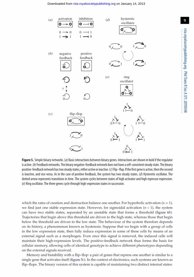
Figure 5. Simple binary networks. (a) Basic interactions between binary genes. Interactions are shown in bold if the regulatoris active. (b) Feedback networks. The binary negative-feedback network does not have a self-consistent steady state. The binarypositive-feedbacknetworkhas two steady states, either active or inactive. (c) Flip–flop. If thefirst gene is active, then the secondis inactive, and vice versa. As in the case of positive feedback, the system has two steady states. (d) Hysteretic oscillator. Thedotted arrow represents transitions in time. The system cycles between states of high activator and high repressor expression.(e) Ring oscillator. The three genes cycle through high-expression states in succession.

which the rates of creation and destruction balance one another. For hyperbolic activation (n = 1),we find just one stable expression state. However, for sigmoidal activation (n > 1), the systemcan have two stable states, separated by an unstable state that forms a threshold (figure 6b).Trajectories that begin above this threshold are driven to the high state, whereas those that beginbelow the threshold are driven to the low state. The behaviour of the system therefore dependson its history, a phenomenon known as hysteresis. Suppose that we begin with a group of cellsin the low expression state, then fully induce expression in some of these cells by means of anexternal signal such as a morphogen. Even once this signal is removed, the induced cells willmaintain their high-expression levels. The positive-feedback network thus forms the basis forcellular memory, allowing cells of identical genotype to achieve different phenotypes dependingon the external signals received.

Memory and bistability with a flip–flop: a pair of genes that repress one another is similar to asingle gene that activates itself (figure 5c). In the context of electronics, such systems are known asflip–flops. The binary version of this system is capable of maintaining two distinct internal states:

on January 14, 2013rsta.royalsocietypublishing.orgDownloaded from

12

rsta.royalsocietypublishing.orgPhilTransRSocA371:20110548

......................................................

2.0

1.5

1.0

0.5

0

1

2

3

2.0

1.5

1.0

0.5

0

2

4

6

6

5

4

3

2

1

6

5

4

3

2

1

0 1 2 3 4 5 6

0 0.5 1.0 1.5 2.0 0 0.5 1.0 1.5 2.02.5

x0 1 2 3 4 5 6

x

x x

y

time

dx / dt

(a) (b)

(c) (d)

(i)

(ii)

(i)

(ii)

Figure6. Continuous feedback networks. (a) Negative feedback. (i) Protein creation anddegradation rates. (1) f(x) = 2/(1 +x) for the auto-repressed system. (2) f(x) = 1 for the unregulated system. (3) g(x) = x. (ii) Solid lines show timecourses forthe auto-repressed system; dashed lines show timecourses for the unregulated system. Negative feedback producesmore rapidequilibration. (b) Positive feedback. (i) Protein creation and degradation rates. (1) For f(x) = 2x/(1 + x), the system has asingle stable fixed point. (2) For f(x) = 2x4/(1 + x4), the system has two stable fixed points, separated by an unstable fixedpoint. (3) g(x) = x. (ii) Timecourses. Systems initialized at x > 1 are driven to the high state, whereas those initialized at x < 1are driven to the low state. (c,d) Flip–flop. Graphs in x–y space show nullclines (solid) and trajectories (dashed) for equation(4.5) with A= 5. (c) For n= 1, the system has one stable state. (d) For n= 4, the system has two stable states, one at high-xlow-y, and the other at high-y low-x.

if we choose one gene to be active, then the other must be inactive. In terms of concentrations,

dxdt

= A1

1 + yn − x ≡ u(x, y)

anddydt

= A1

1 + xn − y ≡ v(x, y).

⎫⎪⎪⎬⎪⎪⎭ (4.5)

To understand system dynamics, it is useful to examine the curves u(x, y) = 0, along whichdx/dt = 0, and v(x, y) = 0, along which dy/dt = 0. The fixed points or steady states of the systemoccur where these curves, known as nullclines, intersect. Once again, we must ask of each fixed

on January 14, 2013rsta.royalsocietypublishing.orgDownloaded from

13

rsta.royalsocietypublishing.orgPhilTransRSocA371:20110548

......................................................

point whether it is stable or unstable. In this case, a graphical analysis shows that, for n = 1,the system has a single stable fixed point along the diagonal x = y (figure 6c). For n > 1, thissymmetric fixed point becomes unstable, and two asymmetric stable fixed points are created,one corresponding to high x-expression, and the other to high y-expression (figure 6d). As in thecase of the positive feedback network, the flip–flop provides a mechanism for cellular memory.

Hysteretic oscillator: we again look at a system of two genes, but now one of them is anactivator, while the other is a repressor (figure 5d). In a sense, this is an extended version ofa negative feedback circuit we saw previously, and the binary model predicts that it shouldoscillate. Importantly, because the feedback now comes with a delay, oscillations can be shownto occur in the corresponding continuous system as well. Consider the following activator–repressor pair:

dxdt

= γx

(vx + Ax

x2

1 + x21

1 + y− x

)≡ u(x, y)

anddydt

= vy + Ayx − y ≡ v(x, y).

⎫⎪⎪⎪⎬⎪⎪⎪⎭ (4.6)

The nullclines intersect at a single fixed point, and the flows suggest oscillatory behaviour. If xis slow to respond to changes in y, this fixed point is stable and any oscillations are damped(figure 7a). However, if x responds sufficiently rapidly, the fixed point becomes unstable, and thesystem enters a sustained limit-cycle oscillation (figure 7b). Hysteretic oscillators of this kind areknown to form the molecular basis for circadian rhythms and other types of periodic phenomenain living cells [46].

Ring oscillator: finally, let us consider a system with three genes, each repressing the next insequence (figure 5e). The binary system is clearly oscillatory. The continuous analogue may bespecified as

dxi

dt= A

11 + xn

i−1− xi, (4.7)

where i = 0 is identified with i = 3. The system has a symmetric fixed point xi = x0. For sufficientlyhigh n, this fixed point can become unstable, forcing the system into a limit-cycle oscillation(figure 7c).

5. Separating biochemistry from topology

(a) Estimating biochemical and topological complexitySuppose we are given N distinct regulatable promoters, each of which has binding sites for up toM distinct transcription factors. In addition, we are given Next promoters whose transcriptionaloutputs can be controlled using extracellular signals. Each promoter can be made to expressone or more transcription factors; the same transcription factor might be expressed by multiplepromoters, in which case its total level is obtained by summing. We assume that the levels ofall transcription factors can be measured. To simplify the discussion, we discretize the system sothat all the inputs and outputs can take on any one of the states x ∈ {0, 1, . . . , Ω − 1} with inputssaturating at the maximal level. Reasonable values of these quantities are N, Next approximately2–10, M ∼ 2–5 [47], and Ω ∼ 10.

A promoter is specified by defining its response to ΩM distinct inputs. For each promoteri, let this information be summarized as a function αi(x1, x2, . . . , xn). The set {αi|i = 1, . . . , N}represents the biochemical specification of the system. There are ΩΩNM

possible biochemistries(though given the continuous and slowly varying nature of a promoter’s input–output function,the accessible biochemical space will in reality be much smaller than this).

We next turn to topology, which involves specifying which of the N + Next promoters is drivingeach of the M inputs of a given promoter. The M × (N + Next) connectivity matrix for promoter i

on January 14, 2013rsta.royalsocietypublishing.orgDownloaded from

14

rsta.royalsocietypublishing.orgPhilTransRSocA371:20110548

......................................................

2.0(i) (ii)

1.5

1.0

0.5

0

0.5 1.0 1.5 0 10 20 30 40

2.0

1.5

1.0

0.5

0

y

y

x time

time

3

2

1

0 5 10 15 20

xi

(a)

(b)

(c)

Figure 7. Continuous oscillators. (a,b) Hysteretic oscillator. We show results for equation (4.6), with vx = 0.1, vy = 0.0,Ax = 4.0, Ay = 2.0. (i) Shows nullclines (solid) and trajectories (dotted) in x–y space. (ii) Shows y(t). (a) For γx = 3.0,oscillations are damped and the system eventually reaches the fixed point. (b) Forγx = 5.0, the fixed point is unstable, and thesystem enters a limit cycle oscillation. (c) Ring oscillator. We show results for equation (4.7), with A= 4 and n= 4. The graphshows the values of x1, x2 and x3 over time. The system eventually enters a limit cycle.

has the form

Cijk =

⎛⎜⎜⎜⎜⎜⎜⎜⎝

M

⎧⎪⎪⎨⎪⎪⎩

N︷ ︸︸ ︷Ci

1,1 . . . Ci1,N

.... . .

...Ci

M,1 . . . CiM,N

∣∣∣∣∣∣∣∣∣∣∣∣∣

Next︷ ︸︸ ︷Ci

1,N+1 . . . Ci1,N+Next

.... . .

...Ci

M,N+1 . . . CiM,N+Next

⎞⎟⎟⎟⎟⎟⎟⎟⎠

, (5.1)

where the indices j and k run over inputs and promoters, respectively; and each entry can take onvalues 0 or 1. The set {Ci|i = 1, . . . , N} represents the topological specification of the system and

on January 14, 2013rsta.royalsocietypublishing.orgDownloaded from

15

rsta.royalsocietypublishing.orgPhilTransRSocA371:20110548

......................................................

there are approximately 2NM(N+Next) possible topologies (ignoring degeneracies). Notice that thebiochemical space explodes much more rapidly than the topological space.

Consider a feedback network constructed with some complicated Cijk. Such a network will

have N′ext ≤ Next external inputs, and therefore can be put into ΩN′

ext configurations. Howcompletely can we probe the biochemistry of such a system? To get a rough idea, let us makethe following simplifying assumptions: for each external configuration, the feedback systemachieves a unique steady state; and as we cycle through configurations, a given promoter cyclesthrough a random sample (with repeats) of its ΩM possible states. The probability that a given

state is missed over ΩN′ext samples is (1 − 1/ΩM)Ω

N′ext ≈ exp(−ΩN′

ext/ΩM). Therefore, the expectednumber of distinct states sampled by each promoter is ΩM(1 − exp(−ΩN′

ext/ΩM)). The depth ofbiochemical characterization is essentially a step function: if N′

ext < M our sampling is extremelysparse; if N′

ext � M we hit nearly all possible states; and with ΩM samples our fractional coverageis (1 − 1/e).

If Next ≥ M, we can choose to construct a synthetic genetic network with the trivial feed-forward architecture (as reported in Rai et al. [26]):

Cijk =

⎛⎜⎜⎜⎜⎜⎜⎜⎝

M

⎧⎪⎪⎨⎪⎪⎩

0 . . . 0...

. . ....

0 · · · 0

∣∣∣∣∣∣∣∣0 . . . 0...

. . ....

0 · · · 0

M︷ ︸︸ ︷1 . . . 0...

. . ....

0 . . . 1

⎞⎟⎟⎟⎟⎟⎟⎟⎠

= (0 | 0I), (5.2)

where 0 is the zero matrix and I is the identity matrix. This allows us to perform a completebiochemical characterization, in which we determine all the functions αi, using exactly ΩM

external configurations. Having done the feed-forward characterization we can, in principle,predict the response of any other topology under all of its ΩN′

ext external configurations.An experimental demonstration of this feed-forward-to-feedback predictive procedure wasreported by Rai et al. [26]. For N′

ext > M, this type of prediction is clearly efficient: a largenumber of feedback responses can be predicted from a relatively small number of feed-forwardmeasurements. However, in practice, it is often the case that even ΩM is large in absolute terms,making a complete biochemical characterization unfeasible.

(b) Case study: bacterial cell-to-cell communicationThere are several natural contexts in which bacterial cells in a population stand to benefitby coordinating their actions [48]. Many bacterial species achieve such coordination throughchemical communication channels that work on the following principle [49]. Any cell in thepopulation can ‘issue’ a signal using an enzyme designated I; this enzyme generates a moleculeknown as acyl-homoserine lactone (AHL) that can diffuse freely between cells. Cells ‘receive’this signal using a transcription factor designated R; when R is bound to AHL it functions asan activator, driving transcription at a promoter henceforth designated pX. The capability of I/Rsystems to issue and receive signals can have a variety of uses [50]. Because the concentrationof AHL in the medium is a readout of the density of cells issuing the signal, one hypothesis isthat these systems allow cells to tune their transcriptional response as a function of populationdensity (figure 8)—hence the term ‘quorum sensing’. For example, cells infecting a host canremain quiescent until they reach a critical density, staying hidden from the host’s immune systemuntil they are ready to launch a virulent attack [51]. Topologically, I/R quorum-sensing systemsare interesting because they are invariably found in a particular positive-feedback configuration:the enzyme I is expressed downstream of the R-dependent promoter pX [26,52].

A computational and experimental characterization of I/R systems has been reportedpreviously [26]. We revisit those results in the context of the biochemical and topologicalframework developed here. The key variables are (figure 8): the bacterial cell density ρ; the

on January 14, 2013rsta.royalsocietypublishing.orgDownloaded from

16

rsta.royalsocietypublishing.orgPhilTransRSocA371:20110548

......................................................

R

I

pX

AHL

r

Figure 8. Schematic of an I/R quorum-sensing system. Cells have number density ρ . The intracellular enzyme I synthesizesthe chemical signal AHL, which diffuses into the medium and subsequently into other cells. The transcription factor R, whenbound to AHL, activates transcription of mRNA at the promoter pX. For clarity, we have separated the ‘issuing’ and ‘receiving’ ofthe chemical signal, but these processes happen simultaneously within each cell.

concentration φ of AHL in the medium; and the intracellular concentrations YI and YR of theenzyme I and transcription factor R. AHL levels will be proportional both to the enzyme levelsand to cell density: φ(t) = μρ(t)YI(t). The transcriptional output of promoter pX is a function ofinstantaneous AHL and R levels. This biochemistry is summarized:

αX(φ, YR) = αX(μρYI, YR). (5.3)

Given two external promoters pA and pB, the system can be wired into the following topologies:

PX PA PB

IR

⎛⎝0 1 0∣∣∣∣

0 0 1

⎞⎠

︸ ︷︷ ︸feed-forward

,

PX PA PB

IR

⎛⎝1 0 0∣∣∣∣

0 1 0

⎞⎠

︸ ︷︷ ︸I-feedback

and

PX PA PB

IR

⎛⎝0 1 0∣∣∣∣

1 0 0

⎞⎠

︸ ︷︷ ︸R-feedback

, (5.4)

where matrices of the format (5.1) specify which promoters are driving which of the two inputsof promoter pX. If the proteins I and R have translation rates QI, QR and decay rates γI, γR,respectively, the feedback systems are described by the following differential equations:

I-feedback1γR

dYR

dt= QRαR − YR

1γI

dYI

dt= QIαX(μρYI, YR) − YI

and R-feedback1γI

dYI

dt= QIαI − YI

1γR

dYR

dt= QRαX(μρYI, YR) − YR.

⎫⎪⎪⎪⎬⎪⎪⎪⎭ (5.5)

Here, αI and αR are control parameters: transcription rates that are constant in time but whosevalues can depend on external inputs; the function αX() embodies the frozen biochemicalparameters; and the structure of the equations indicates the feedback topology. There areevidently two reasons why the responses of R-feedback and I-feedback systems might differ. Thefirst is biochemical: the promoter logic αX(μρYI, YR) is an asymmetric function of its two inputsYI and YR (figure 9a). The second is structural or topological: the input YI is multiplied by thecell density, whereas the input YR is fed in directly (figure 9b,c) causing these two variables toinfluence the dynamics in completely distinct ways.

If cell density varies slowly compared with intracellular protein concentrations, equation (5.5)can be solved to obtain quasi-steady-state values YI and YR as functions of ρ. Under positivefeedback, two distinct classes of responses can arise (figure 10a). For monostable responses(type M; mnemonic sMooth), transcription increases smoothly with cell density. For bistableresponses (type B; mnemonic aBrupt), there is a range of cell densities over which two stable

on January 14, 2013rsta.royalsocietypublishing.orgDownloaded from

17

rsta.royalsocietypublishing.orgPhilTransRSocA371:20110548

......................................................

10 000

1000

100

10

10 100 1000 10 000

YI

YR

YR

aI

YR

aR

aX aX

YI

¥ r

YI

¥ r

f

0.99

0.10

0.01

(a) (b) (c)

Figure 9. I/R feedback systems. (a) The input–output function of pX : the output transcription rate as a function of YI andYR at a fixed cell density ρ . The contour plot shows the value of αX(μρYI , YR), as measured in Rai et al. [26]. (b,c) Feedbacktopologies. Either R or I is controlled externally, while the other protein is expressed from the promoter pX with transcriptionrate αX(μρYI , YR). The same promoter can also drive further outputs. The two topologies are different because the functionαX () is asymmetric, and because it is only the term YI that is multiplied by the cell densityρ . (b) R-feedback. (c) I-feedback.

1.0

0.5

0 0 0 00.05 0.05 0.05 0.05

M B + B ± B –

B ±

B –

r r r r

1

10–1

10–2

10–3

aRaI

0 0.5 1.0 1.5 2.0n

0 0.5 1.0 1.5 2.0n

outp

ut

R feedback I feedback

MB +

B ±

B –

M

B +

(a)

(b)

Figure 10. Density-dependent responses. (a) Four types of responses: (M)monostable, where transcription smoothly increaseswith cell density; (B+) bistable,with a threshold density atwhich transcription abruptly increases; (B±) bistable andhystereticat the terminal density, where high and low transcription states coexist; (B−) bistable but uninduced even at the terminaldensity, since the potentially bistable region is never reached. (b) Regions of {α, n} space that generate each response type;αrepresents the external control parameter, whereas n represents the Hill coefficient based on a parametrization of the input–output functionαX(μρYI , YR) [26].

transcription levels coexist. For each topology, a bifurcation analysis can be used to obtain regionsof parameter space that give rise to the different response types [26, supporting information].Figure 10b shows a two-dimensional slice of the parameter space: a biochemical parameter n (theHill coefficient of R-DNA binding, which plays a key role in determining the form of αX()) isvaried along the x-axis; the control parameters αI or αR are varied along the y-axis. We see thatthe R-feedback topology is constrained: it is restricted to a single response type independent ofthe regulator level, once biochemical parameters are frozen. However, the I-feedback topologyis versatile: it can be tuned between smooth and abrupt density-dependent response types byvarying the regulator alone. This versatility might underlie the observed preference for I-feedbacksystems among diverse bacterial species: an organism that is able to rapidly modify its response inthe face of an uncertain and fluctuating environment gains a crucial fitness advantage. Versatility

on January 14, 2013rsta.royalsocietypublishing.orgDownloaded from

18

rsta.royalsocietypublishing.orgPhilTransRSocA371:20110548

......................................................

B±

1

10–1

10–2

10–3

aI

0 0.5

M B+

B±

1

10–1

10–2

10–3

aR

0 0.5

M

R-feedback

I-feedback

B+

B–

n1.0

1.5 2.0

biochemistryregu

latio

n

topology

I-A

II-A

1-B

(a) (b)

Figure 11. Using topology to tame biochemistry. (a) Regulation, biochemistry and topology can each be used to modulate theresponse of a genetic network, but on successively longer time scales. (b) We show a slice of biochemical space in which twonetwork topologies (I and II) can potentially generate two different types of responses (A and B) within the regions indicated.Grey dots represent the unknown, a priori distribution of parameter values. Although region I-B appears larger than region I-A,topology-I is much more likely to generate type A responses compared with type B responses because of the increased densityof dots in region I-A. However, because region I-A completely contains region II-A, we can say that topology-I is more likely togenerate type A responses than topology-II is, regardless of the density of dots.

is a purely topological property of the system, made without reference to specific biochemicalparameter values.

6. ConclusionThere are three types of changes that can be used to modulate the response of genetic networks,operating on completely distinct time scales (figure 11a). Control parameters (such as thetranscription rates αI or αR) are the software: they can respond directly and dynamically to externalinputs, and vary on time scales from minutes to hours. Biochemical parameters (such as the Hillcoefficient n) are the firmware: they can be changed incrementally by mutations, infrequent eventsthat might become fixed in a population only over hundreds of generations. Network topology isthe hardware: it is possible to switch topology but this requires rare, potentially disruptive, large-scale DNA rearrangements. The topological hardware and biochemical firmware are essentiallyfrozen, leaving only the regulated software to vary freely at short time scales.

When studying natural genetic networks, the approach to take depends on the extent ofavailable data. If topology is known and key parameters identified, we can use experimentalmeasurements to constrain as many parameters as feasible. Of the remaining parameters we cantry to identify a few that are expected to be critical, and investigate all possible system behavioursas their values are varied. This approach is incomplete, however, because of a further unknownthat is often ignored: we rarely, if ever, know the a priori distribution of parameter values that arelikely to occur in nature. It is therefore impossible to estimate or compare the volumes of regionsin parameter space that give rise to any set of specified behaviours (such as A or B; figure 11b).Even in this situation, topology provides a useful organizing framework. Consider the region ofparameter space of some genetic network associated with some desired behaviour. If this regionin the case of topology-II is completely contained within that in the case of topology-I, thenwe can be certain that the topology-I is more likely to generate the desired behaviour, without

on January 14, 2013rsta.royalsocietypublishing.orgDownloaded from

19

rsta.royalsocietypublishing.orgPhilTransRSocA371:20110548

......................................................

knowing anything about the likelihood of occurrence of parameters (figure 11b). The analysisthus generates a partial ordering among topologies independent of the actual biochemistry, andsuggests a means to search the space of all possible topologies for interesting networks. Searchingthrough topologies in this manner might be the only approach possible if the very existenceof certain interactions is in doubt. For each topology, we would scan over parameter values toidentify the range of possible behaviours. It could be the case that several topologies are consistentwith some desired outcomes. In that case, it might be necessary to add additional biologicallyrelevant constraints: robustness to parameter variation; adaptation to external changes; powerconsumption efficiency; and so on. The approach of searching topological space with constraintsis emerging as a powerful means to understand the design principles of complex genetic networksin the absence of detailed biochemical data [53–58].

We might soon achieve a nearly complete understanding of certain simple organisms througha systematic analysis of the networks that govern their behaviour. Eventually such techniquesmight even give us predictive power, allowing us to guess at the inner workings of organismsbased solely on the annotated sequences of their genomes. However, on very long time scales,the structure of a network must itself be dynamic: natural selection can be thought of as driving asearch through topological space, converging on network architectures that generate biologicallyuseful outcomes [59,60]. As more and more genome sequences enter the databases, we can beginto catalogue regularities in network architecture, or striking differences between different species.Once enough such patterns are known, it might be possible to shift our focus away from thequestion that concerned us here, of what genetic networks do, towards the broader question ofhow such networks came to be.

This work was supported in part by a WellcomeTrust–DBT India Alliance Intermediate Fellowship(500103/Z/09/Z). I thank Sandeep Krishna for discussions about the utility of topological descriptions, andRajat Anand for help in preparing figures. Sections 1–4 and related figures are adapted, with permission, from‘The dynamics of genetic networks’ by M. Thattai, c© 2004 Massachusetts Institute of Technology. Portions of§5 and related figures are adapted, with permission, from ‘Prediction by promoter logic in bacterial quorumsensing’ by N. Rai, R. Anand, K. Ramkumar, V. Sreenivasan, S. Dabholkar, K. V. Venkatesh and M. Thattai,PLoS Comput. Biol. 8, e1002361, c© 2012 Rai et al.

References1. Monod J. 1966 From enzymatic adaptation to allosteric transition. Science 154, 475–483.

(doi:10.1126/science.154.3748.475)2. Alberts B, Johnson A, Lewis J, Raff M, Roberts K, Walter P. 2007 Molecular biology of the cell, 4th

edn. New York, NY: Garland Science.3. Hobert O. 2008 Gene regulation by transcription factors and microRNAs. Science 319,

1785–1786. (doi:10.1126/science.1151651)4. Bansal M, Belcastro V, Ambesi-Impiombato A, di Bernardo D. 2007 How to infer gene

networks from expression profiles. Mol. Syst. Biol. 3, 78. (doi:10.1038/msb4100120)5. Hu Z, Killion PJ, Iyer VR. 2007 Genetic reconstruction of a functional transcriptional

regulatory network. Nat. Genet. 39, 683–687. (doi:10.1038/ng2012)6. Bonneau R. 2008 Learning biological networks: from modules to dynamics. Nat. Chem. Biol. 4,

658–664. (doi:10.1038/nchembio.122)7. Balleza E, López-Bojorquez LN, Martínez-Antonio A, Resendis-Antonio O, Lozada-Chávez

I, Balderas-Martínez YI, Encarnación S, Collado-Vides J. 2009 Regulation by transcriptionfactors in bacteria: beyond description. FEMS Microbiol. Rev. 33, 133–151. (doi:10.1111/j.1574-6976.2008.00145.x)

8. MacQuarrie KL, Fong AP, Morse RH, Tapscott SJ. 2011 Genome-wide transcription factorbinding: beyond direct target regulation. Trends Genet. 27, 141–148. (doi:10.1016/j.tig.2011.01.001)

9. Thieffry D, Huerta AM, Perez-Rueda E, Collado-Vides J. 1998 From specific gene regulation togenomic networks: a global analysis of transcriptional regulation in Escherichia coli. BioEssays20, 433–440. (doi:10.1002/(SICI)1521-1878(199805)20:5<433::AID-BIES10>3.0.CO;2-2)

on January 14, 2013rsta.royalsocietypublishing.orgDownloaded from

20

rsta.royalsocietypublishing.orgPhilTransRSocA371:20110548

......................................................

10. Lee TI et al. 2002 Transcriptional regulatory networks in Saccharomyces cerevisiae. Science 298,799–804. (doi:10.1126/science.1075090)

11. Faith JJ, Hayete B, Thaden JT, Mogno I, Wierzbowski J, Cottarel G, Kasif S, Collins JJ, GardnerTS. 2007 Large-scale mapping and validation of Escherichia coli transcriptional regulation froma compendium of expression profiles. PLoS Biol. 5, e8. (doi:10.1371/journal.pbio.0050008)

12. Zhu J, Zhang B, Smith EN, Drees B, Brem RB, Kruglyak L, Bumgarner RE, Schadt EE. 2008Integrating large-scale functional genomic data to dissect the complexity of yeast regulatorynetworks. Nat. Genet. 40, 854–861. (doi:10.1038/ng.167)

13. Barabasi A, Albert R. 1999 Emergence of scaling in random networks. Science 286, 509–512.(doi:10.1126/science.286.5439.509)

14. Shen-Orr S, Milo R, Mangan S, Alon U. 2002 Network motifs in the transcriptional regulationnetwork of Escherichia coli. Nat. Genet. 31, 64–68. (doi:10.1038/ng881)

15. Alon U. 2007 Network motifs: theory and experimental approaches. Nat. Rev. Genet. 8,450–461. (doi:10.1038/nrg2102)

16. Alleyne TM et al. 2009 Predicting the binding preference of transcription factors to individualDNA k-mers. Bioinformatics 8, 1012–1018. (doi:10.1093/bioinformatics/btn645)

17. Siddharthan R. 2010 Dinucleotide weight matrices for predicting transcription factor bindingsites: generalizing the position weight matrix. PLoS ONE 5, e9722. (doi:10.1371/journal.pone.0009722)

18. Yang S, Yalamanchili HK, Li X, Yao KM, Sham PC, Zhang MQ, Wang J. 2011 Correlatedevolution of transcription factors and their binding sites. Bioinformatics 27, 2972–2978.(doi:10.1093/bioinformatics/btr503)

19. Shea MA, Ackers GK. 1985 The OR control system of bacteriophage lambda: aphysical-chemical model of gene regulation. J. Mol. Biol. 181, 211–230. (doi:10.1016/0022-2836(85)90086-5)

20. Ozbudak EM, Thattai M, Lim HN, Shraiman BI, van Oudenaarden A. 2004 Multistabilityin the lactose utilization network of Escherichia coli. Nature 427, 737–740. (doi:10.1038/nature02298)

21. Buchler NE, Gerland U, Hwa T. 2003 On schemes of combinatorial transcriptional logic. Proc.Natl Acad. Sci. USA 100, 5136–5141. (doi:10.1073/pnas.0930314100)

22. Setty Y, Mayo AE, Surette MG, Alon U. 2003 Detailed map of a cis-regulatory input function.Proc. Natl Acad. Sci. USA 100, 7702–7707. (doi:10.1073/pnas.1230759100)

23. Cox 3rd RS, Surette MG, Elowitz MB. 2007 Programming gene expression with combinatorialpromoters. Mol. Syst. Biol. 3, 145. (doi:10.1038/msb4100187)

24. Kaplan S, Bren A, Zaslaver A, Dekel E, Alon U. 2008 Diverse two-dimensional input functionscontrol bacterial sugar genes. Mol. Cell 29, 786–792. (doi:10.1016/j.molcel.2008.01.021)

25. Tamsir A, Tabor JJ, Voigt CA. 2011 Robust multicellular computing using genetically encodedNOR gates and chemical ‘wires’. Nature 469, 212–215. (doi:10.1038/nature09565)

26. Rai N, Anand R, Ramkumar K, Sreenivasan V, Dabholkar S, Venkatesh KV, Thattai M. 2012Prediction by promoter logic in bacterial quorum sensing. PLoS Comput. Biol. 8, e1002361.(doi:10.1371/journal.pcbi.1002361)

27. Tan C, Marguet P, You L. 2009 Emergent bistability by a growth-modulating positive feedbackcircuit. Nat. Chem. Biol. 5, 842–848. (doi:10.1038/nchembio.218)

28. Hertz J, Krogh A, Palmer RG. 1991 Introduction to the theory of neural computation. Reading,MA: Perseus Books.

29. Minsky ML, Papert SA. 1969 Perceptrons. Cambridge, MA: MIT Press.30. Arcas BA, Fairhall AL, Bialek W. 2003 Computation in a single neuron. Neural Comput. 15,

1715–1749. (doi:10.1162/08997660360675017)31. Lawrence PA. 1992 The making of a fly. Oxford, UK: Blackwell Scientific.32. Tyson JJ, Chen KC, Novak B. 2003 Sniffers, buzzers, toggles and blinkers: dynamics of

regulatory and signaling pathways in the cell. Curr. Opin. Cell Biol. 15, 221–231. (doi:10.1016/S0955-0674(03)00017-6)

33. Alon U. 2007 An introduction to systems biology: design principles of biological circuits. Boca Raton,FL: Chapman & Hall.

34. Hasty J, McMillen D, Collins JJ. 2002 Engineered gene circuits. Nature 420, 224–230.(doi:10.1038/nature01257)

35. Purnick PEM, Weiss R. 2009 The second wave of synthetic biology: from modules to systems.Nat. Rev. Mol. Cell Biol. 10, 410–422. (doi:10.1038/nrm2698)

on January 14, 2013rsta.royalsocietypublishing.orgDownloaded from

21

rsta.royalsocietypublishing.orgPhilTransRSocA371:20110548

......................................................

36. Khalil AS, Collins JJ. 2010 Synthetic biology: applications come of age. Nat. Rev. Genet. 11,367–379. (doi:10.1038/nrg2775)

37. Becskei A, Serrano L. 2000 Engineering stability in gene networks by autoregulation. Nature405, 590–593. (doi:10.1038/35014651)

38. Dublanche Y, Michalodimitrakis K, Kümmerer N, Foglierini M, Serrano L. 2006 Noise intranscription negative feedback loops: simulation and experimental analysis. Mol. Syst. Biol.2, 41. (doi:10.1038/msb4100081)

39. Becskei A, Seraphin B, Serrano L. 2001 Positive feedback in eukaryotic gene networks: celldifferentiation by graded to binary response conversion. EMBO J. 20, 2528–2535. (doi:10.1093/emboj/20.10.2528)

40. Isaacs FJ, Hasty J, Cantor CR, Collins JJ. 2003 Prediction and measurement of anautoregulatory genetic module. Proc. Natl Acad. Sci. USA 100, 7714–7719. (doi:10.1073/pnas.1332628100)

41. Gardner TS, Cantor CR, Collins JJ. 2000 Construction of a genetic toggle switch in Escherichiacoli. Nature 403, 339–342. (doi:10.1038/35002131)

42. Atkinson MR, Savageau MA, Myers JT, Ninfa AJ. 2003 Development of genetic circuitryexhibiting toggle switch or oscillatory behavior in Escherichia coli. Cell 113, 597–607.(doi:10.1016/S0092-8674(03)00346-5)

43. Stricker J, Cookson S, Bennett MR, Mather WH, Tsimring LS, Hasty J. 2008 A fast, robust andtunable synthetic gene oscillator. Nature 456, 516–519. (doi:10.1038/nature07389)

44. Elowitz MB, Leibler S. 2000 A synthetic oscillatory network of transcriptional regulators.Nature 403, 335–338. (doi:10.1038/35002125)

45. Paulsson J. 2003 Summing up the noise in gene networks. Nature 427, 415–418.(doi:10.1038/nature02257)

46. Tyson JJ, Albert R, Goldbeter A, Ruoff P, Sible J. 2008 Biological switches and clocks. J. R. Soc.Interface 5(Suppl. 1), S1–S8. (doi:10.1098/rsif.2008.0179.focus)

47. Nam J, Dong P, Tarpine R, Istrail S, Davidson EH. 2010 Functional cis-regulatory genomics forsystems biology. Proc. Natl Acad. Sci. USA 107, 3930–3935. (doi:10.1073/pnas.1000147107)

48. Wingreen NS, Levin SA. 2006 Cooperation among microorganisms. PLoS Biol. 4, e299.(doi:10.1371/journal.pbio.0040299)

49. Waters CM, Bassler BL. 2005 Quorum sensing: cell-to-cell communication in bacteria. Annu.Rev. Cell Dev. Biol. 21, 319–346. (doi:10.1146/annurev.cellbio.21.012704.131001)

50. Hense BA, Kuttler C, Muller J, Rothballer M, Hartmann A, Kreft JU. 2007 Doesefficiency sensing unify diffusion and quorum sensing? Nat. Rev. Microbiol. 5, 230–239.(doi:10.1038/nrmicro1600)

51. de Kievit TR, Iglewski BH. 2000 Bacterial quorum sensing in pathogenic relationships. Infect.Immun. 68, 4839–4849. (doi:10.1128/IAI.68.9.4839-4849.2000)

52. Smith D et al. 2006 Variations on a theme: diverse N-acyl homoserine lactone-mediatedquorum sensing mechanisms in Gram-negative bacteria. Sci. Prog. 89, 167–211. (doi:10.3184/003685006783238335)

53. François P, Hakim V. 2004 Design of genetic networks with specified functions by evolutionin silico. Proc. Natl Acad. Sci. USA 101, 580–585. (doi:10.1073/pnas.0304532101)

54. Klemm K, Bornholdt S. 2005 Topology of biological networks and reliability of informationprocessing. Proc. Natl Acad. Sci. USA 102, 18 414–18 419. (doi:10.1073/pnas.0509132102)

55. Ciliberti S, Martin OC, Wagner A. 2007 Innovation and robustness in complex regulatory genenetworks. Proc. Natl Acad. Sci. USA 104, 13 591–13 596. (doi:10.1073/pnas.0705396104)

56. Avlund M, Dodd IB, Sneppen K, Krishna S. 2009 Minimal gene regulatory circuits that cancount like bacteriophage lambda. J. Mol. Biol. 394, 681–693. (doi:10.1016/j.jmb.2009.09.053)

57. Ma W, Trusina A, El-Samad E, Lim WA, Tang C. 2009 Defining network topologies that canachieve biochemical adaptation. Cell 138, 760–773. (doi:10.1016/j.cell.2009.06.013)

58. Burda Z, Krzywicki A, Martin OC, Zagorski M. 2011 Motifs emerge from function in modelgene regulatory networks. Proc. Natl Acad. Sci. USA 108, 17 263–17 268. (doi:10.1073/pnas.1109435108)

59. Babu MM, Luscombe NM, Aravind L, Gerstein M, Teichmann SA. 2004 Structure andevolution of transcriptional regulatory networks. Curr. Opin. Struct. Biol. 14, 283–291.(doi:10.1016/j.sbi.2004.05.004)

60. Oikonomou P, Cluzel P. 2006 Effects of topology on network evolution. Nat. Phys. 2, 532–536.(doi:10.1038/nphys359)

on January 14, 2013rsta.royalsocietypublishing.orgDownloaded from