using the two-period model to understand investment … · 2017-07-13 · using the two-period...

National Tax Journal, March 2017, 70 (1), 185–204

USING THE TWO-PERIOD MODEL TO UNDERSTAND INVESTMENT IN HUMAN CAPITAL

M. Daniele Paserman

In many textbooks, the decision to invest in human capital is presented in terms of the present discounted value of the lifetime stream of costs and benefits associated with the investment. I argue that this approach, while delivering some useful in-sights, also conflates subjective discount rates and market interest rates, obfuscates the role of credit market imperfections, and makes difficult the analysis of policy interventions and the effects of external shocks on human capital investment. I show instead how a simple two-period model can deliver the main insights about investment in human capital and is flexible enough to be used to model a wide variety of policy interventions.

Keywords: human capital, capital market imperfections, time preferences, stu-dent loans

JEL Codes: A20, A22, D90, H31, I26, I28

I. INTRODUCTION

At the core of every investment decision is a tradeoff between costs in the present and benefits that materialize in the future. This tradeoff also holds for the case of

investment in human capital. Most textbooks describe the decision about whether to invest in human capital as one that involves simply the calculation of the net present discounted value of the stream of all costs and benefits associated with the investment. In this paper, I argue that this simple approach suffers from two major shortcomings: (1) it conflates the notion of a subjective discount rate and the market interest rate; and (2) it obfuscates the role of borrowing and credit market imperfections. Thus, it makes difficult any analysis of the response of human capital investment to policy or macroeconomic changes, such as subsidized student loans or changes in the return to education.

Instead, I show how one can illustrate the basic principles of the human capital investment decision using a two-period model, a simple adaptation of the two-good

M. Daniele Paserman: Department of Economics, Boston University, Boston, MA, USA, and National Bureau of Economic Research, Cambridge, MA, USA ([email protected])

https://doi.org/10.17310/ntj.2017.1.08

National Tax Journal186

consumption model that will be familiar to any undergraduate with a basic background in intermediate microeconomics. The investment decision is presented as one in which a prospective student derives utility from “present” (period 0) and “future” (period 1) consumption and must choose between two alternative combinations of present and future income. One is a “college” path that has low income in the present and high income in the future, and the other is a “no college” path that has relatively high income in the present but also lower income in the future. These two alternative paths yield different budget constraints. The investment decision problem can then be broken down into two parts: (1) find the optimal combination of present and future consumption on each of the two budget constraints; and (2) choose the income profile that yields maximum global utility.

It is instructive to start with the case of perfect capital markets, where the student is assumed to be able to lend and borrow any amount at the given market interest rate. In this case, it is easy to see that only one of three cases is possible: either the “college” budget constraint strictly dominates the “no college” budget constraint, or “no col-lege” strictly dominates “college,” or the two budget constraints are exactly identical. The investment decision boils down to choosing the income profile with the highest present discounted value, as in the traditional approach. One can also introduce the concept of the internal rate of return (IRR) of college investment as the interest rate that would make the net present value of the two income profiles equivalent. It is easy to illustrate the IRR graphically and derive the familiar result from finance classes that the Net Present Value (NPV) criterion and the IRR criterion yield exactly the same investment decision rule. Importantly, with perfect capital markets, the investment decision does not depend on the shape of indifference curves: regardless of whether an individual is patient or impatient, she will always choose either to invest in college or to not invest. Therefore, differences in human capital investment by demographic or socioeconomic groups cannot be explained by differences in subjective discount rates.

More interesting is the case with imperfect capital markets, by which I mean any situation in which the interest rate for borrowers is different from (and typically, much higher than) the interest rate for lenders. In this case, the budget constraints exhibit a kink at the income endowment point, and in general a strict ranking of the “college” and “no college” income profiles is no longer possible. Now, the decision to invest in col-lege depends not only on the pecuniary returns to the investment, but also on individual preferences: investment in college is more likely by students with flatter indifference curves (i.e., students with a lower marginal rate of substitution between present and future consumption, and who are therefore more future oriented).

Having laid out the framework of the model, the paper goes on to show how it can be used to evaluate the effect of a number of different macroeconomic shocks (such as the secular increase in the returns to schooling) and policy interventions (subsidiz-ing tuition, expanding access to student loans, or subsidizing interest rates on student loans). These applications can help the student understand some of the recent trends

Using the Two-Period Model to Understand Investment in Human Capital 187

in college enrollment and student debt, and assess the effectiveness of several policies that are currently at the center of the public debate.

The advantages of this approach to modeling the human capital investment decision are manifold. First, it allows the student to analyze the problem of human capital investment using the familiar graphical tools of indifference curves and budget constraints. Second, it introduces conceptual clarity by distinguishing between the role of the subjective discount rate and the market interest rate. This distinction makes it possible to overcome some of the logical inconsistencies that arise when trying to explain cross-sectional differences in investment as a function of differences in the subjective discount rate. Finally, it models credit market imperfections in a straightforward way, allowing one to easily analyze the effect of policy interventions in the area of student loans.

The rest of the paper is structured as follows. The first section will survey the way in which the human capital investment decision is typically presented in most labor and public economics textbooks, and it highlights some related shortcomings. The follow-ing section will introduce the two-period model and the budget constraint faced by a prospective college student in the case of perfect capital markets. I will then move to the case of imperfect capital markets and discuss some pedagogical tools that can be used to illustrate the differences between market interest rates and subjective discount rates. Finally, I will show how the model can be applied to address a number of important and policy-relevant questions.1

II. THE PRESENT VALUE APPROACH

The traditional model used to illustrate the human capital investment decision is based on the concept of present value. As with any other form of investment, investment in human capital involves a comparison of costs that are typically borne in the present with benefits that will occur at a later date. In the case of the schooling decision, the current costs include: (1) the direct costs associated with schooling (including tuition, fees, books and supplies, but excluding room and board, which would have to be incurred even if one did not attend school); (2) the foregone earnings that arise because one cannot work, or at least not work full time, when attending school; and (3) any non-pecuniary costs associated with schooling. The benefits are the increased future earnings and any other nonpecuniary benefits associated with a higher level of schooling or attending college. Because these benefits mostly materialize in the future, the question arises as to how one should compare one dollar received today with one dollar received in the future.

The traditional textbook explanation (and one that most undergraduates understand quite readily) is that a dollar received today is more valuable than one received in the

1 Potential confusion between different concepts of the discount rate appears also in other areas in economics. Most prominent is the debate in climate policy about how much weight should be given to the utility of future generations, and whether the market interest rate provides good guidance for this parameter (Stern, 2008; Nordhaus, 2007); see Kaplow, Moyer, and Weisbach (2010) for a general discussion.


future, because it can be invested and earn a positive rate of interest. Specifically, if the interest rate is 3 percent, $100 dollars today are equivalent to $103 received a year from now, or, alternatively, the present value of $100 received a year from today is $97.09 (100/1.03 = 97.09). More generally, with a constant interest rate r, any amount Bt obtained t years from today has a present value of Bt /(1 + r)t. Then, the present value of the lifetime stream of benefits associated with investment in schooling is simply

(1) =

++

++ +

+PV B

Br

Br

Br

( )1 (1 ) (1 )

,TT

1 22

where T is the length of the horizon. The Net Present Value (NPV) of the investment is defined as NPV = PV(B) – C, where C is the initial outlay.2 An individual will choose to invest in schooling if the present value exceeds the initial outlay or, equivalently, if NPV > 0.

As is well known, an equivalent method to evaluating whether an investment is worthwhile is based on the Internal Rate of Return (IRR). The IRR is the discount rate r* such that

(2) − ++

++

+ ++

=CBr

Br

Br1 * (1 *) (1 *)

0.TT

1 22

The IRR tells us the minimum discount rate that would still make the investment have a positive net present value. If the IRR exceeds the market interest rate on alter-native investments (or the interest rate paid on borrowing), then the investment is profitable.

The NPV method has some pedagogical advantages. First, it clearly focuses the students on the notion of opportunity costs. One of the main components of the costs of attending school is the opportunity cost of foregone earnings. Moreover, the calcula-tion also makes clear that benefits that materialize in the future need to be discounted, because of the opportunity cost of otherwise investing the money elsewhere. Second, the NPV formula delivers clear and straightforward predictions on some of the key determinants of the schooling investment decision. An individual is more likely to invest if the benefits from attending school are larger, if the costs are lower, and if the time horizon over which the returns to investment are reaped is longer. Third, the NPV and IRR methods feature prominently in a number of different areas of economics and are likely to be used extensively by students in many of the jobs they will pursue after graduation. Therefore, it is particularly useful to expose students to these concepts for a highly relevant decision problem, and with which they are familiar. Finally, it is straightforward to illustrate numerically the NPV calculation using actual data on earn-ings of college and high school graduates, and thus to provide a preliminary answer to the popular question, “is college worth it?” The Excel file in the online supplementary

2 Somewhat more generally, costs may be incurred for more than just the initial year. The same discount rate can then be used to calculate the present value of costs, PV(C), in which case NPV = PV(B) – PV(C).


Appendix provides one such calculation using data from the 2013 and 2014 American Community Survey.3

The NPV method, however, also has some significant pedagogical shortcomings. First, most presentations of the NPV formula tend to conflate the market interest rate and the subjective discount rate, the rate at which individuals are willing to trade off between current and future consumption. As described above, the justification typi-cally given for discounting future income streams is that $100 earned one year from now is less valuable than $100 earned today, because the latter can be invested and earn a positive rate of interest. This explanation clearly implies that that the discount rate r used in the NPV formula should be equivalent to the market interest rate (inci-dentally, one might wonder what exactly the “market” interest rate is: the interest rate on checking and savings account, on certificates of deposit, on short term government bonds, or some other rate?), but then r should not be related to an individual’s rate of time preference. One cannot argue that individuals will differ in their college investment decisions because of the way in which they value intertemporal tradeoffs. Yet, most leading textbooks in the market appear to jump seamlessly between the notion of the discount rate as a market interest rate and as a subjective discount rate. For example, Ehrenberg and Smith (2012), in explaining the concept of present value, clearly argue that future benefits payments should be discounted at the market interest rate:

… [A] woman is offered $100 now or $100 in a year. Would she be equally attracted to these two alternatives? No, because if she received the money now, she could either spend (and enjoy) it now, or she could invest the $100 and earn interest over the next year. If the interest rate were 5 percent, say, $100 now could grow into $105 in a year’s time. (Ehrenberg and Smith, 2012, pp. 280–281)

Only a few pages later, however, the concept of the discount rate is no longer related to the market interest rate, and instead reflects an individual’s intertemporal preference:

Although we all discount the future somewhat with respect to the present, psychologists use the term present-oriented to describe people who do not weight future events or outcomes very heavily … [A] present-oriented person is one who uses a very high discount rate (r). (Ehrenberg and Smith, 2012, pp. 285–286)

3 Any reasonable estimate of the costs and benefits of college shows that the NPV is large and positive, and has been growing over time (Avery and Turner, 2012). This of course would be a good place also to point out some of the caveats with this analysis: (1) the simple comparison of earnings between high school graduates and college graduates does not necessarily imply that the relationship is causal; (2) the calculation only shows information on average returns and ignores the substantial heterogeneity across the population; and (3) as every good investment prospectus reminds us, “past performance is no guar-antee of future performance.” The online Appendix is available at http://people.bu.edu/paserman/papers/ Paserman_UsingTwoPeriodModel_NTJ2017_SupplementaryMaterials.zip.


A similar inconsistency appears in Borjas (2010). The concept of present value is described using an example almost identical to that of Ehrenberg and Smith, i.e., equat-ing the discount rate to the market interest rate. But a few pages later, we read

… [T]he rate of discount r plays a crucial role in determining whether a per-son goes to school or not. The worker goes to school if the rate of discount is 5 percent but does not if the rate of discount is 15 percent. The higher the rate of discount, therefore, the less likely a worker will invest in education... A worker who has a high discount rate attaches a very low value to future earnings opportunities — in other words, he discounts the receipt of future income ‘too much’ …

It is sometimes assumed that the person’s rate of discount equals the market rate of interest, the rate at which funds deposited in financial institutions grow over time. After all, the discounting of future earnings in the present value calculations arises partly because a dollar received this year can be invested and is worth more than a dollar received next year.

The rate of discount however, also depends on how we feel about giving up some of today’s consumption in return for future rewards — or our ‘time preference.’ Casual observation…suggests that people differ in how they approach this trade-off. Some of us are ‘present oriented’ and some of us are not. Persons who are present oriented have a high discount rate and are less likely to invest in schooling. (Borjas, 2010, p. 242)4

It appears that Borjas (2010) is arguing that the discount rate is some combination of the market interest rate and the subjective rate of time preference. But the two concepts are distinct, and it can be confusing to students to have them merged together. If people facing high market interest rates invest less in education, then a policy of low interest rates would be effective in stimulating investment in human capital. This policy, how-ever, is much less likely to be effective if low investment in human capital is driven by a high level of the subjective discount rate. The distinction is also important if one wants to understand cross-sectional differences in education. If one believes that low socio-economic status individuals have fewer financial investment opportunities and therefore

4 Other textbooks also fail to make the distinction between market interest rates and subjective discount rates. Hyclak, Johnes, and Thornton (2013) equate the discount rate to the market interest rate, with no discussion at all about subjective impatience. Laing (2011) does the same, even though he devotes one whole section to imperfect capital markets and how they affect the investment decision. In his exposition, heterogeneity in investment derives from heterogeneity in borrowing costs, not in rates of time preference. McConnell, Brue, and Macpherson (2013) equate the discount rate to the market interest rate, but do discuss time preferences in a footnote, arguing present-oriented individuals effectively use a high interest rate to discount future flows of earnings.


their rate of return on alternative investments is lower, it would follow that educational investments should be higher for people with a low socioeconomic background.5 If, on the other hand, wealth causes patience, as hypothesized by Becker and Mulligan (1997), we would observe the opposite relationship: high socioeconomic status individuals invest more in schooling, as is indeed the case (National Center for Education Statistics, 2015).

A second shortcoming of the NPV approach is that it is completely silent about the possibility that students may need to borrow to finance their educational investment. In the model, the prospective student is essentially assumed to have at her disposal enough capital to pay all direct costs of college in full — the question boils down to one of whether to allocate this capital to finance one’s own education or to invest it in an alternative channel. Without explicitly modeling the borrowing decision, it becomes difficult to analyze the factors that have contributed to the dramatic increase in student debt over the past 15 years, and the policy interventions that could be used to facilitate access to college or to ease the burden of debt repayment and to reduce insolvency. These include, but are not limited to, subsidized interest rates for student loans, deferred repayment plans, income contingent repayment plans, and many more. A more flexible approach to modeling the schooling investment decision is needed.6

III. THE TWO-PERIOD MODEL

The factors affecting the human capital investment decision can be more clearly understood using a two-period model, a simple adaptation of the two-good consumption model that will be familiar to any undergraduate with a basic background in interme-diate microeconomics. The main insights can be derived using simple graphical tools. Despite its simplicity, the model is highly flexible, and can be used to address many of the questions raised in the previous section.

A. The Two-Period Model

We assume that an individual lives two periods, denoted zero (“the present”) and one (“the future”), and derives utility from an aggregate consumption good in each of the periods, C0 and C1. We can depict the amount consumed of both goods on a traditional

5 A more plausible scenario is that low socioeconomic status individuals have less access to borrowing, and therefore are offered loans with higher interest rates. But remember that in the present value formula, the discount rate represents the rate of return on alternative investments. In the following section we will introduce the possibility that the interest rates for borrowers and for lenders differ.

6 In principle, one could modify the NPV formula to allow for borrowing, but the formula becomes quickly quite cumbersome. Specifically, assume that a student takes on $D of debt, at interest rate rB

, which must be repaid within TD periods, starting from period 1. Then, the NPV formula becomes

∑∑= − − + − + + += +=

NPV C D B p r B r( ) ( ) / (1 ) / (1 )tt

tt

t T

T

t

T

11 D

D , where = − + − p r D r T/ 1 (1 )B B D is the

constant repayment amount. As in the traditional calculation, the question about the appropriate discount rate r remains unresolved.


two-dimensional graph, with C0 on the horizontal axis and C1 on the vertical axis. In its most general form, the utility function can be written as U(C0,C1). Indifference curves have the usual shape and properties, i.e., they are downward sloping and convex (Figure 1). It may be useful at this point to remind students that the slope of the indif-ference curve represents the marginal rate of substitution between present and future consumption, i.e., the amount of future consumption that one is willing to give up to gain an extra unit of present consumption and remain indifferent. Hence, a steeper indifference curve represents an individual with more present-oriented preferences — she is willing to give up more future consumption to gain an additional unit of present consumption.7

The individual receives an endowment of monetary income: Y0 in period 0 and Y1 in period 1. The individual wishes to maximize utility subject to a budget constraint, whose shape depends on the assumptions we make about the nature of the capital market.

C1

C0

UA

UB

Figure 1Indifference Curves

Notes: The figure depicts two representative indifference curves for two individuals, A and B. Individual A, who has the steeper indifference curve, is more present-oriented.

7 For more advanced students, it may be useful here to discuss the additively separable utility function that is used pervasively in economics: ρ= + +U C C u C u C( , ) ( ) ( ) / (1 )0 1 0 1 . This explicit formulation is useful because it clearly shows how the subjective discount rate r is a parameter of the utility function.


We start from the benchmark assumption of perfect capital markets, meaning that the individual can borrow or lend any amount at a constant interest rate r. In this case, the budget constraint takes on the usual form

(3) ++

= ++

CCrY

Yr1 1.0

10

1

For students, it can be instructive to derive the budget constraint step by step. First, note that the endowment point (Y0, Y1) is always necessarily on the budget constraint. The individual can always choose to consume her endowment, without borrowing or lending at all. What happens if the individual wants to reduce her current consumption by one dollar? She can put that dollar in the bank where it will accumulate interest, and therefore increase future consumption by (1 + r) dollars. Alternatively, if the individual wants to increase consumption today by one dollar, she must borrow that amount and therefore reduce future consumption by (1 + r) dollars. In other words, the budget con-straint always goes through the endowment point (Y0, Y1) and has slope equal to (1 + r) (Figure 2a). The derivation of the slope of the budget constraint also illustrates that the “price” of one extra unit of consumption today is (1 + r) units of consumption tomor-row. Hence, we have the familiar result that the slope of the budget constraint is equal to the price ratio between C0 (“good X,” on the horizontal axis) and C1 (“good Y,” on the vertical axis). The budget constraint also has the intuitive interpretation that the present value of the consumption stream must be equal to the present value of the income stream.

More realistically, capital markets are not perfect, and there will typically be a wedge between the interest rate available to lenders and to borrowers. This is a good place to ask students to compare between the interest rates on their checking or savings accounts, and that on their student loans or credit cards. Even those who are not very financially sophisticated will immediately realize that the gap is quite substantial.8 In terms of our model, the difference in the interest rate for lending (rL) and the interest rate for bor-rowing (rB , with rB > rL) generates a kink in the budget constraint: the endowment point (Y0, Y1) is always available to the consumer, but now the slope of the budget constraint to the right of the endowment point, where the individual borrows from the future to finance higher consumption today, is higher than the slope to the left of the endowment point, where the individual reduces consumption today to save for the future (Figure 2b).

With perfect capital markets, the optimal consumption bundle is achieved at the point where the slope of the budget constraint (one plus the market interest rate) is equal to the slope of the indifference curve (one plus the subjective rate of discount). With imperfect capital markets, one also needs to pay attention to the kink point. If the slope of the indifference curve at the kink point is lower than (1 + rB) and greater than (1 + rL), then the kink point is the optimal consumption bundle.

8 As of the writing of this article (October 2016), the interest rate on checking and savings account is less than 0.1 percent, the interest rate on three-month Treasury bills is 0.32 percent, the interest rate on 15-year mortgages is about 3.0 percent, the interest rate on subsidized undergraduate loans is 4.66 percent, and the interest rate on credit card debt varies between 15 and 22 percent.


B. Modeling the College Decision

It is straightforward to use this model to analyze the decision to go to college. College is a form of investment in human capital, whereby the individual foregoes some level of current income to raise her future income. If the individual chooses not to attend col-lege, she earns income Y0,NC in the present and Y1,NC in the future. If she attends college, she earns income (net of tuition and other direct expenses associated with college) Y0,C in the present, and Y1,C in the future, with Y0,C < Y0,NC and Y1,C > Y1,NC. In terms of the two-period model, the individual’s choice is a choice between two endowment points (points EC and ENC in Figure 3). Given the endowment point, the individual maximizes her lifetime utility subject to her budget constraint. The decision to attend college is one of choosing the endowment point that will yield the highest lifetime utility.

1. Perfect Capital Markets

Start by considering the case of perfect capital markets. Using the graph, it is easy to show that one choice will always strictly dominate the other, depending on the slope of the budget constraint. If the interest rate is relatively low, the budget constraint associated with College will lie strictly above the budget constraint associated with No College (Figure 4A), and the individual will unambiguously choose to attend col-lege. Conversely, with a high interest rate and a relatively steep budget constraint, the

Panel A Panel B

C1

C0

Y1

C1

Y1

Y0

1 + r

1 + rL

1 + rB

Y0

Y0

Figure 2Budget Constraint with Perfect and Imperfect Capital Markets

Notes: Panel A shows the shape of the budget constraint in the case of perfect capital markets, i.e., when individuals can borrow and lend any amount at the constant interest rate r. Panel B shows the budget constraint when the interest rate for borrowing rB is greater than the interest rate for lending rL.


individual will unambiguously choose No College (Figure 4B). Notice that these results hold regardless of the shape of the individual’s indifference curves. In other words, in a world with perfect capital markets, the individual’s degree of time preference is com-pletely irrelevant for the decision to attend college or not. Instead, the decision depends critically on the market interest rate: when the interest rate is low, the alternative to attending college (i.e., not attending and putting some of the relatively high current income in the bank) is not very attractive, and the individual chooses to attend college. The opposite is true if the interest rate is high.

It is thus clear that the individual chooses the college option if point EC lies on a higher budget line than point ENC . This is equivalent to saying that the present discounted value of endowment point EC is higher than the present discounted value of point ENC. Mathematically,

(4) ++

> ++

YYrY

Yr1 1.C

CNC

NC0,

1,0,

1,

We are back to the original result described in Section II: choose to attend college if the present value of attending college is higher than the alternative. However, as shown below, this result hinges critically on the assumption of perfect capital markets. In other words, the present value approach gives the correct answer on the investment choice

Figure 3Endowment Points for College and No College

C1

C0

Y1.C

Y1,NC

ENC

EC

Y1,NCY0,C


only under the highly implausible assumption that there is no difference in interest rates for borrowing and lending.

Finally, one can calculate the level of the interest rate that would make an individual indifferent between choosing the college and no-college paths. Setting the present discounted value of the two paths equal, and solving for r*, we have

(5) ++

= ++

=−−

−YYr

YYr

rY YY Y1 * 1 *

* 1.CC

NCNC C NC

NC C0,

1,0,

1, 1, 1,

0, 0,

Note that because r* is defined as the interest rate that makes the individual indif-ferent between the college and the no college path, it is effectively the internal rate of return of the college investment. Again, with perfect capital markets, the criterion for investing in college boils down to traditional IRR criterion: invest in college if the internal rate of return is higher than the alternative interest rate. The IRR criterion is illustrated graphically in Figure 5.

2. Imperfect Capital Markets

The case of perfect capital markets provides a benchmark for understanding how the college investment decision is affected by the rate of return to college attendance and by market interest rates. However, we need to relax this assumption for a more complete

Panel A Panel B

C1

C1C0

Y1.C

Y1,NC

C1

Y1.C

Y1,NCENCENC

EC EC

Y0,NCY0,C Y0,NCY0,C

Figure 4The College Choice with Perfect Capital Markets

Notes: Panel A shows the shape the budget constraints associated with the College and No College choices with perfect capital markets, and a relatively low interest rate. The College choice strictly dominates. Panel B shows the budget constraints when the interest rate is relatively high. In this case, the No College choice dominates.

⇒


analysis. This allows us to understand more fully the role of time preferences, and also makes it possible to evaluate the effect of different policy interventions.

Figure 6 illustrates graphically the budget constraints associated with the College and No College options in the case of imperfect capital markets, with rL < rB.

As is clear from Figure 6, it is no longer the case that one budget set strictly dominates the other. The decision whether to attend college will depend on the exact shape of the indifference curves. An individual with indifference curve UA chooses to attend college, while an individual with indifference curve UB chooses not to attend. (In Figure 6, both individuals choose exactly the kink point, but this does not necessarily have to be the case). Note that A’s indifference curve is generally flatter than B’s indifference curve: at any point, individual A has a lower marginal rate of substitution between future and present consumption, meaning that she is willing to give up a smaller amount of consump-tion tomorrow to increase her consumption today.9 In other words, A is more patient or more future-oriented, and she is more likely to attend college than B. As in Ehrenberg and Smith (2012) and Borjas (2010), we obtain the result that more future-oriented individuals are more likely to attend college. For example, Ehrenberg and Smith (2012)

1 + r *

C1

C0

Y1,C

Y1,NC

ENC

EC

Y0,NCY0,C

Figure 5The Internal Rate of Return of College Investment

Notes: The internal rate of return of investing in college is the interest rate r * such that the dashed line going through points EC and ENC has slope 1 + r *.

9 More precisely, on any vertical line that crosses both indifference curves, the slope of B’s indifference curve is steeper than the slope of A’s indifference curve.


1 + r B

1 + r L

C0

C1

Y1,C

Y1,NCENC

UA

UB

EC

Y0,NCY0,C

argue that the evidence of a positive correlation between health outcomes and education is suggestive that some of the cross-sectional differences in college attendance is due to differences in subjective discount rates. The two-period model makes clear the condi-tions under which this result holds, and it introduces conceptual clarity by distinguishing between the market interest rate and the subjective discount rate.

To further sharpen this distinction for students, it may be useful to conduct the fol-lowing hypothetical survey:

Question 1:

Option A: $100 in cash today.Option B: $100 + x in cash a year from now.What is the value of x that would make you indifferent between options A and B?

Question 2:

Option A: A $100 gift certificate to be used at your favorite restaurant today. The gift certificate has your name and today’s date on it, so it is not tradeable and can only be used today.Option B: A ($100 + y) gift certificate to be used at your favorite restaurant exactly one year from now. The same conditions as above apply.What is the value of y that would make you indifferent between options A and B?

Figure 6The College Decision with Imperfect Capital Markets


The two questions appear similar, but elicit fundamentally different concepts. Ques-tion 1 may reflect both time preferences and market interest rates. Some students may report a particularly high value of x (say, $50), but you can probably cause them to reconsider by offering to loan them $100 if they agree to repay you $140 a year from now (assuming that this contract is strictly enforceable). In fact, many students will give values of x that approach the market interest rate, probably influenced by the notion (acquired in previous classes) that $100 today is worth $100(1 + r) a year from now, because one can always put the money in the bank and earn interest. Question 2, on the other hand, makes clear that the tradeoff really is between consumption today and a year from now. The value of y is likely greater than zero because of uncertainty (will the restaurant still be in existence a year from now, will the chef still be as good, will the items on the menu be the same, will prices stay the same?). The value of y is also likely greater than zero because of impatience — I would rather consume a good meal today than wait a year. The market interest rate has nothing to do with the decision.10

IV. APPLICATIONS

The two-period model lends itself well to analyzing the effects of various policies and shocks on college enrollment rates. In what follows, I use the model to show how these choices respond to an increase in the returns to schooling, a change in tuition, an expansion in student loans, and a student-loan interest-rate subsidy. I provide in the online Appendix some examples of problem set questions that build on these ideas. For simplicity, I assume throughout that students are allowed to borrow up to a cap D, that the interest rate on student loans is rD (with rD > rL ), and that no other borrowing is allowed (this is an extreme version of imperfect capital markets, with rB → ∞). The budget set associated with college is the thin black line AEC FG in Figure 7. The slope of the budget line is 1 + rL on the segment AEC , and 1 + rD on the segment ECF. The horizontal distance between EC and F represents the loan cap amount D.

A. Increase in Returns to Schooling

The gap in earnings between workers with and without a college degree has increased dramatically over the past 35 years (Acemoglu and Autor, 2011). What is the effect of such a development on the propensity to attend college, and on the debt that students incur?11 An increase in the returns to schooling can be modeled as an increase in Y1,c, holding everything else constant (Figure 7). The budget constraint for the college option shifts upward, from AECFG to A′EC′F′G. The figure depicts the indifference curve for an individual who, prior to the increase in the returns to schooling, chooses not to attend college (point ENC lies on a higher indifference curve than any point on the Col-lege budget constraint). The increase in post-college earnings induces this individual

10 The difficulty that one sometimes encounters with Question 2 is that some undergraduate students struggle to imagine themselves spending $100 at a restaurant!

11 I present the increase in returns to schooling as an external shock, perhaps driven by changes in technology or trade. Of course, one can always view this same shock as a policy that lowers taxes on high earners.


to attend college instead, and to choose a point like F ′ (which involves borrowing, to get from the endowment point EC′ to the consumption point F ′). On the other hand, people who chose college before the increase in returns to schooling will continue to choose college. The increase in returns to schooling, not surprisingly, makes attending college more attractive.

Also, what happens to student debt? Some students who previously were not enrolled in college choose college instead and start borrowing. In addition, some students who previously chose to attend college but did not borrow (for example, a student who chose point EC on the old budget constraint) may now move to a point between EC′ and F ′, where they do borrow. Finally, students who previously chose to attend college and did borrow (i.e., students who chose a point between EC and F ) will now continue to attend college and borrow at least as much as they did previously (under the assumption that both present and future consumption are normal goods — this may be a good place to remind students of income and substitution effects!). The bottom line is that student debt unambiguously increases, even though one can presume that the higher earnings of college graduates would make default less likely.12

Figure 7Increase in Returns to Schooling

C0

C1

Y1′,C

Y1,C

Y1,NCENC

A′

A

UB

E ′C

ECF ′

F

G

Y0,NCY0,C

12 Unfortunately, one of the shortcomings of the two-period model is that there is no way to model default or other outcomes that depend on the longer run, such as a restructuring of debt payments.


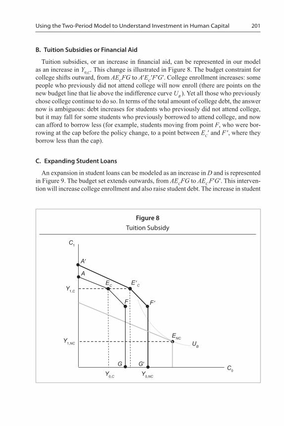
B. Tuition Subsidies or Financial Aid

Tuition subsidies, or an increase in financial aid, can be represented in our model as an increase in Y0,C. This change is illustrated in Figure 8. The budget constraint for college shifts outward, from AECFG to A′EC′F′G′. College enrollment increases: some people who previously did not attend college will now enroll (there are points on the new budget line that lie above the indifference curve UB ). Yet all those who previously chose college continue to do so. In terms of the total amount of college debt, the answer now is ambiguous: debt increases for students who previously did not attend college, but it may fall for some students who previously borrowed to attend college, and now can afford to borrow less (for example, students moving from point F, who were bor-rowing at the cap before the policy change, to a point between EC′ and F ′, where they borrow less than the cap).

C. Expanding Student Loans

An expansion in student loans can be modeled as an increase in D and is represented in Figure 9. The budget set extends outwards, from AECFG to AEC F′G′. This interven-tion will increase college enrollment and also raise student debt. The increase in student

Figure 8Tuition Subsidy

C0

C1

Y1,C

Y1,NC

A′

A

UB

E ′C

ENC

EC

F ′F

G G′

Y0,NCY0,C


Figure 9Expansion in College Loans

Figure 10Student Loan Interest Rate Subsidies

C0

C1

Y1,C

Y1,NC

A

UB

ENC

EC

F ′

F

G G′Y0,C

C0

C1

Y1,C

Y1,NC

A

UB

ENC

EC

F ′

F

GY0,C Y0,NC


debt comes from two sources: (1) students who previously did not attend college can now borrow and attend; and (2) those who were already going to college and borrowing at the cap can now borrow more.

D. Subsidized Interest Rates on Student Loans

Finally, we consider the effect of subsidized interest rates on student loans. The policy is represented in Figure 10 below. The budget set expands from AECFG to AEC F′G. This policy also raises college enrollment, as some students who previously chose no college now prefer the college option with lower interest rates on loans. We can again say that this policy unambiguously increases debt, as some students who previously did not enroll in college now enroll and borrow. Among those who previously enrolled and borrowed, income and substitution effects both operate in the direction of increas-ing present consumption and borrowing more (a move from point F to a point on the EC F′ segment).

V. CONCLUSION

Human capital plays a central role in many theories of the labor market and in many other areas. Any theory of human capital investment should be able to explain the fac-tors that determine why some people invest heavily in their schooling while others do not. The traditional way in which the human capital investment decision is presented in most undergraduate textbooks is based on the notion of maximizing the net present value of the investment decision, and this approach delivers some useful insights. But it also leads to some conceptual confusion, and it does not lend itself well to analyzing the effects of policy interventions and macroeconomic changes. This is an important shortcoming especially in the current climate, where the issue of college affordability and student debt is at the center of the policy debate, both in the United States and abroad.

In this paper, I show how the schooling decision can be illustrated using a simple two-period model that does not require any additional analytical tools beyond those acquired in any intermediate microeconomics course. The model can flexibly accom-modate the realistic scenario of credit-constrained students, and it is easy to use to derive the implications of a variety of policy interventions in the student loan market. Given the relevance of the material for most students, this topic usually generates a large amount of classroom engagement and discussion. Instructors can draw from the online Appendix for additional materials, including an Excel spreadsheet that can be used to calculate the present value of college investment, as well as sample problems sets and lecture note slides.

ACKNOWLEDGMENTS AND DISCLAIMERS

I would like to thank George Borjas, Don Fullerton, and Robert Smith for helpful comments. All errors are my own.


DISCLOSURES

The author has no financial arrangements that might give rise to conflicts of interest with respect to the research reported in this paper.

REFERENCES

Acemoglu, Daron, and David Autor, 2011. “Skills, Tasks and Technologies: Implications for Employment and Earnings.” In Ashenfelter, Orley, and David Card (eds.), Handbook of Labor Eco-nomics, Volume 4B, 1043–1171. North-Holland Publishing Company, Amsterdam, Netherlands.

Avery, Christopher, and Sarah Turner, 2012. “Student Loans: Do College Students Borrow Too Much — Or Not Enough?” Journal of Economic Perspectives 26 (1), 165–192.

Becker, Gary S., and Casey B. Mulligan, 1997. “The Endogenous Determination of Time Prefer-ence.” Quarterly Journal of Economics 112 (3), 729–758.

Borjas, George J., 2010. Labor Economics: Fifth Edition. McGraw-Hill Education, New York, NY.

Ehrenberg, Ronald G., and Robert S. Smith, 2012. Modern Labor Economics: Theory and Public Policy, Eleventh Edition. Prentice Hall, Upper Saddle River, NJ.

Hyclak, Thomas, Geraint Johnes, and Robert Thornton, 2013. Fundamentals of Labor Economics, Second Edition. Cengage Learning, Boston, MA.

Kaplow, Louis, Elisabeth Moyer, and David A. Weisbach, 2010. “The Social Evaluation of Inter-generational Policies and its Application to Integrated Assessment Models of Climate Change.” B.E. Journal of Economic Analysis and Policy 10 (2), 1–32.

Laing, Derek, 2011. Labor Economics. W.W. Norton & Company, New York, NY.

McConnell, Campbell R., Stanley L. Brue, and David A. Macpherson, 2013. Contemporary Labor Economics: Tenth Edition. McGraw-Hill, New York, NY.

National Center for Education Statistics, 2015. “Postsecondary Attainment: Differences by Socioeconomic Status.” National Center for Education Statistics, Washington, DC, http://nces.ed.gov/programs/coe/indicator_tva.asp.

Nordhaus, William D., 2007. “A Review of the Stern Review on the Economics of Climate Change.” Journal of Economic Literature 45 (3), 686–702.

Stern, Nicholas, 2008. “The Economics of Climate Change.” American Economic Review 98 (2), 1–37.

using the two-period model to understand investment … · 2017-07-13 · using the two-period...

Documents