https://ntrs.nasa.gov/search.jsp?R=20080015431 2018-07-09T11:04:22+00:00Z

h

Using the Bootstrap Method for aStatistical Significance Test of Differences

Between Summary Histograms

Kuan-Man Xu

NASA Langley Research Center, Hampton, VA

Submitted to Monthly Weather Review

January 4, 2005Revised, May 31, 2005

Accepted, September 29, 2005

Corresponding author address:Dr. Kuan-Man XuClimate Science BranchNASA Langley Research CenterMail Stop 420Hampton, VA 23681e-mail: Kuan-Man.Xu@nasa.gov

1

Abstract

A new method is proposed to compare statistical differences between summary histo-

grams, which are the histograms summed over a large ensemble of individual histograms. It con-

sists of choosing a distance statistic for measuring the difference between summary histograms

and using a bootstrap procedure to calculate the statistical significance level. Bootstrapping is an

approach to statistical inference that makes few assumptions about the underlying probability dis-

tribution that describes the data. Three distance statistics are compared in this study. They are the

Euclidean distance, the Jeffries-Matusita distance and the Kuiper distance.

The data used in testing the bootstrap method are satellite measurements of cloud systems

called “cloud objects.” Each cloud object is defined as a contiguous region/patch composed of

individual footprints or fields of view. A histogram of measured values over footprints is gener-

ated for each parameter of each cloud object and then summary histograms are accumulated over

all individual histograms in a given cloud-object size category. The results of statistical hypothe-

sis tests using all three distances as test statistics are generally similar, indicating the validity of

the proposed method. The Euclidean distance is determined to be most suitable after comparing

the statistical tests of several parameters with distinct probability distributions among three cloud-

object size categories. Impacts on the statistical significance levels resulting from differences in

the total lengths of satellite footprint data between two size categories are also discussed.

2

1. Introduction

In atmospheric and oceanic sciences, the amount of data created from observational and

modeling studies is enormous. Satellite measurements can produce a few gigabytes of data a day.

High-resolution global climate modeling can easily produce a similar amount of data for a

monthly simulation. There are a few possible methods to analyze the large amount of data. One is

to average the individual satellite footprint (or field of view) data over a large region and over an

extended period so that climate signals are adequately sampled. A similar averaging is also often

taken in the climate modeling community. This allows a direct comparison between observations

and models so that possible deficiencies of model simulations can be identified. However, this

approach does not provide direct clues for improving model simulations because of cancellation

of errors in the averaging. Another method is to present observational and modeling data in histo-

grams for each characteristic or parameter to be measured and modeled. This method drastically

reduce the data volume because the data volume is only determined by the bin size of the histo-

gram regardless the size of the original data. A significant advantage of this method is that physi-

cal clues can be found by comparing model simulations with observations if the data are

adequately stratified, for example, according to cloud system types (Xu et al. 2005).

There are many other examples of modeling and observational comparisons that use the

histogram representation. For example, Luo et al. (2003) compared the statistical properties of cir-

rus clouds from cloud-resolving model simulations with ground-based cloud radar measurements.

Cloud-resolving models explicitly resolve the cloud-scale dynamics with parameterized micro-

physics, turbulence and radiation. The cirrus properties were represented in Luo eta al. (2003) by

histograms of cloud thickness, cloud base and top heights and cloud temperature, etc. Due to large

differences between modeled and observed cirrus cloud properties, no vigorous statistical testing

was used to gauge the magnitudes of the differences. This has been the case in many similar

observational and modeling studies (e.g., Dong and Mace 2003; Sengupta et al. 2004). When the

differences between two histograms are not visually large, it is necessary to design a vigorous sta-

tistical testing, for example, to address how closely two histograms resemble to each other.

3

Many statistical methods have been used to analyze observational data and modeling out-

put and to compare the similarities and differences between observational and modeling results in

the atmospheric and oceanic sciences (Wilks 1995). To quantify the similarities and differences,

statistical significance tests are commonly used to judge, for example, whether or not the means

of two time series (or data samples) are statistically different, whether or not two time series are

correlated, and whether or not a regression function fits the data adequately. A parametric distri-

bution of the sample is often assumed so that a simple mathematical expression can be used for

the statistical significance test, for example, the student t-test for sample mean and chi-square test

for sample standard deviation if the parametric distribution is normal. If the distribution of the

population is not known, if it is different from the normal distribution, or if the sample size of the

data is small, computationally intensive methods have to be used to perform the statistical signifi-

cance test, such as the permutation procedure and the bootstrap method (Efron 1982; Livezey and

Chen 1983; Zwiers 1990; Efron and Tibshirani 1993; Gong and Richman 1995; Briggs and Wilks

1996; Wilks 1996, 1997; Chu and Wang 1997; Bove et al. 1998; Beersma and Adri Buishand

1999; Hamill 1999; Chu 2002; Sardeshmukh et al. 2000; McFarquhar 2004).

This particular type of statistical significance test is better known as “statistical hypothesis

test,” a procedure for evaluating, to a certain required level of significance, the null hypothesis

that two sets of data samples are drawn from the same population distribution function. But this

procedure cannot determine that two sets of data samples come from a single distribution. A null

hypothesis constitutes a specific logical frame of reference between a hypothesized value and an

observed value of the test statistic. The test statistic can be any characteristic of the sample. A sta-

tistical hypothesis test consists of calculating the probability of obtaining a statistic that is as dif-

ferent or more different from the null hypothesis than the statistic obtained in a sample for which

the null hypothesis is correct. If this probability value ( value) is sufficiently low, the difference

between the parameter and the statistic is said to be statistically significant; that is, the null

hypothesis is rejected. The level of significance, , is customarily chosen to be 0.05 or 0.01 in the

literature. The value is the probability that one will reject the null hypothesis when it is true,

p

α

α

4

which is called “Type I error.” If one fails to reject the null hypothesis when the null hypothesis is

in fact not true, which is called “Type II error.” The probability (called the value in the litera-

ture) for making the Type II error diminishes as the sample size increases, but it is very difficult to

determine it.

Statistical hypothesis tests have been widely used to explore physical insights of observa-

tions and to evaluate model performance and improvement in many subfields of the atmospheric

and oceanic sciences (e.g., Chu and Wang 1997; Wilks 1997; Bove et al. 1998; Hamill 1999). As

mentioned earlier, information from cloud observation and modeling data can be presented as a

histogram for each characteristic or parameter of a particular cloud system from measurements

made in grids, the points of which are referred to as footprints (or fields of view) in satellite

remote sensing and grid boxes in cloud-resolving modeling. Combining information from several

observed/simulated cloud systems requires combining these histograms into a summary histo-

gram. Summary histograms, which represent signals of combined data samples of observed/simu-

lated cloud systems, can then be compared to each other to infer the statistical behavior of a large

ensemble of cloud systems in different places at different times and in different climatological

conditions or about the performance of a particular cloud-resolving model. Statistical comparison

of histograms can be a robust approach to evaluating and improving cloud-resolving models using

observational data because it is much more difficult for cloud-resolving models to be tuned to

expect improvement in their performance when large numbers of cases are used, compared to that

obtained using a limited number of cases. A detailed discussion of this topic can be found in Xu et

al. (2005) and Eitzen and Xu (2005).

As mentioned previously, it is necessary to decide whether any apparent difference

between histograms is statistically significant. The usual methods of deciding statistical signifi-

cance when comparing histograms do not apply in this case because they assume that the data are

independent. For example, satellite footprint observations or cloud-resolving model output data

are spatially correlated within a cloud system/object. A cloud object is defined as a contiguous

region/patch composed of individual footprints that satisfy a set of physically-based selection cri-

β

5

teria. It is possible to design a method to remove this spatial correlation within a cloud object or

system (e.g. Zwiers 1990; Wilks 1996; Ebisuzaki 1997). By doing so, the goal of combining large

numbers of cloud objects/systems to diagnose climatic signals with small amplitudes (Xu et al.

2005) cannot be achieved. Therefore, a new method is necessary to perform statistical analyses of

large numbers of cloud objects/systems. The objective of this study is to present a new method for

comparing the statistical differences between summary histograms using statistical hypothesis

testing. The proposed method consists of choosing a distance statistic for measuring the differ-

ence between summary histograms and using a bootstrap procedure (Efron and Tibshirani 1993)

to calculate the statistical significance level. Three distance statistics will be extensively com-

pared in this study using satellite cloud-object data.

Section 2 introduces the basics of the bootstrap procedure. Section 3 discusses the detailed

method of comparing histograms. Data used in this study and results are shown in Section 4. Sec-

tion 5 gives a summary and discussion.

2. Basics of the bootstrap procedure

The bootstrap is an approach to statistical inference that makes few assumptions about the

underlying probability distribution that describes the data (Efron 1982; Efron and Tibshirani

1993). This approach assumes that the empirical cumulative distribution function is a reasonable

estimate of the unknown cumulative distribution function of the population. That is, the empirical

density function approximates the population density function. Using the data as an approxima-

tion to the population density function, data are resampled randomly with replacement from the

observed sample, i.e. generating uniform random numbers to draw data from the observed sam-

ple, to create an empirical sampling distribution for the test statistic under consideration. If one

knew the population density function, e.g. the normal probability distribution function (PDF), one

could just sample from this PDF, as in a Monte Carlo simulation, and then generate the sampling

distribution to within any degree of precision. Due to the lack of this information, one has to

assume that the data are a good estimate of the population density function.

6

Specifically, the empirical cumulative distribution function of the data is a step function,

taking jumps of height 1/n at each of the sample points. As n increases, the function becomes

smooth, and looks more like the population cumulative distribution function, and it converges to

the population cumulative distribution function as n approaches infinity. In the bootstrap proce-

dure, the data sample is used as a proxy for the population. That is, one resamples with replace-

ment to produce another data set whose length is equal to the length of the original data sample.

This resampling scheme is known as bootstrap resampling, and the resampled data sets are known

as bootstrap samples. In this procedure, bootstrap samples may contain duplicate copies of the

original data points.

For statistical hypothesis testing, two sets of data are usually used. A test statistic is cho-

sen based upon the null hypothesis to be tested. For example, the null hypothesis is that these two

sets of data are from a distribution with the same mean value, and the alternative hypothesis is that

they are not. Under the null hypothesis, the two samples are from the same distribution, so merg-

ing the samples yields an approximation of the underlying distribution. The bootstrap resampling

procedure is then performed to calculate the probability of obtaining a statistic that is as different

or more different from the null hypothesis than the statistic obtained from the two samples for

which the null hypothesis is correct. If this probability value is sufficiently low, the null hypothe-

sis is rejected. A level of significance of 5% is most often used. It is important to note that it is

possible for bootstrapping to yield incorrect results, specifically, the Type I and Type II errors

mentioned in Section 1. However, this fact is true of any statistical hypothesis test procedure.

An alternative statistical testing procedure is the permutation procedure, in which each

sample is drawn randomly only once without replacement from the merged data. Similar to the

bootstrap procedure, the permutation procedure does not need to make any assumptions of the

sample distribution. Each sample is randomly chosen from the merged data set by a uniform ran-

dom number generator, but each sample in the merged data set is labeled and can only be drawn

once. Two randomized data sets are then formed. This process is repeated many times to calculate

the probability of obtaining a statistic that is as different or more different from the null hypothe-

7

sis than the statistic obtained from the two samples for which the null hypothesis is correct. In

many applications, this procedure yields similar results as the bootstrap procedure (e.g., Livezey

and Chen 1983; Livezey et al. 1997). This will also be verified by the results shown in Section 4.

3. Statistical significance test of the difference between summary histograms

Statistical hypothesis tests can be used to detect statistically significant differences

between summary histograms, which are the histograms summed over a large ensemble of indi-

vidual histograms. These tests seem to be more complicated than some simple examples given in

the literature because the data samples discussed subsequently are composed of many individual

histograms (Fig. 1) with different lengths of data. However, the key aspect in the procedure being

outlined below is to choose the test statistic for measuring the difference/dissimilarity of summary

histograms, which is also the case for cluster analysis as extensively discussed in Gong and Rich-

man (1995). Xu et al. (2005) and Eitzen and Xu (2005) briefly discussed a procedure similar to

that discussed in detail below. In particular, three test statistics are chosen and compared in detail.

First, a distance statistic is chosen to represent the difference between summary histo-

grams. Three distance statistics are tested in this study. They are the Euclidean distance, the Jef-

fries-Matusita (JM) distance, and the Kuiper (Kp) distance. The Euclidean distance measures the

root-mean-square difference between histograms, which is also called the L2 distance. This dis-

tance statistic is defined as

(1),

where f and g are two histograms, with a total of N bins where the ith bin is located at xi. The bin

width is assumed to be uniform and denoted by . The frequency of occurrence is normalized

by the bin width. That is, f and g satisfy . The maximum possible

value of L2 is , and occurs for two single-point histograms that are not collocated.

L2 = f xi( )∆x g xi( )∆x–[ ] 2

i 1=

N

∑

1/2

∆x

f xi( )∆xi 1=

N

∑ g xi( )∆xi 1=

N

∑ 1= =

2

8

The Jeffries-Matusita (JM) distance is also commonly used and is designed to find small

differences in the bins with small probability densities (Matusita 1955). It is successfully used in

pattern classification and image retrieval (e.g. Duda and Hart 1973; Cha and Srihari 2002) and is

defined as

(2).

The values of JM are usually higher than those of L2, as shown in Section 4c, because it gives

more weight to the differences at the tails of histograms with small densities than those obtained

from the L2 distance. However, the maximum possible value of JM is also , as in L2.

The Kolmogorov-Smirnov (KS) distance and its closely related Kuiper distance have

often been used in the atmospheric and oceanic sciences for many different applications (e.g.

Gong and Richman 1995; Anderson and Stern 1996; Sardeshmukh et al. 2000; Gille and Llewel-

lyn Smith 2000; Gille 2004). The KS distance is determined by the maximum value of the abso-

lute difference between two cumulative density functions. It can be expressed by

where i = 1, 2, ... , N (3).

As seen from (3), the KS distance statistic does not integrate over the entire range of histogram

bins. This is fundamentally different from the L2 or JM distance statistics. The Kuiper distance

statistic (Kuiper 1960) overcomes this deficiency slightly by including the contribution from the

tails of the probability distributions, which is defined as

, where i = 1, 2, ... , N (4).

This distance statistic measures the sum of the maximum distances of accumulative above and

below accumulative . It does not integrate over the entire range of histogram bins, either. The

difference between the KS and Kuiper distances is very small from the calculations performed by

JM= f xi( )∆x g xi( )∆x–[ ]2

i 1=

N

∑

1/2

2

KS=Maxi f xi( ) g xi( )– ∆x1

i

∑

Kp=Maxi f xi( ) g xi( )–{ }1

i

∑ Maxi g xi( ) f xi( )–{ }1

i

∑+

f

g

9

the author (not shown). Therefore, only the testing results of the Kuiper distance statistic will be

discussed later. The maximum possible values of KS and Kp are 1.

Second, the bootstrap procedure (Efron and Tibshirani 1993) is used to determine whether

the difference between summary histograms of a particular parameter is statistically significant. A

statistically significant difference between summary histograms means the individual histograms

forming the summary histograms came from two different populations. Each cloud object is com-

posed of many adjacent footprints in a contiguous region/patch (see Section 4a for further details).

There are several parameters measured at each footprint. Each histogram is calculated from the

measurements of the particular parameter of all footprints in a cloud object. Individual histograms

of the top-of-the atmosphere (TOA) albedo and cloud top heights shown in Fig. 1 exhibit large

variabilities, compared to summary histograms shown in Figs. 2d and e. Furthermore, the number

of footprints for calculating the histogram varies from one cloud object to another.

It is assumed that cloud objects, but not their individual footprints, are independent from

each other. That is, the histogram of measured values of a particular parameter is not related to

that of another cloud object. This assumption can be justified because cloud objects occur in dif-

ferent locations and at different times and their histograms of measured parameters are very dif-

ferent from each other (Fig. 1; Xu et al. 2005). An argument could, however, be made that the

cloud objects are dependent based on similar dynamics over a large geographic region where

many cloud objects are developed and maintained. Any dependency involved would be very diffi-

cult to quantity. On the other hand, the individual satellite footprints within a cloud object, as

mentioned earlier, are highly correlated with each other. This is because each footprint occupies

an area of a cloud object that is smaller than a relatively homogenous patch within a cloud object,

but not small enough to reveal finer-scale details within the relatively homogenous patch.

The null hypothesis for the bootstrap procedure or the permutation procedure is that all

cloud objects came from the same population for a particular parameter of the measurements,

which allows the merging of two cloud-object populations for bootstrap or permutation resam-

pling. That is, the choice of which cloud objects were from population A and which were from

10

population B was equivalent to a random choice from the merged data set. Therefore, the distance

between the histograms for the “true” ordering is essentially a random number picked from the

sampling distribution of the bootstrapped distances.

Specifically, the two data sets of m and n cloud objects are first combined into one popula-

tion for a particular parameter at a time in this study. For example, one of the data sets is com-

posed of cloud objects occurred in the eastern Pacific while the other is composed of cloud

objects occurred in the western Pacific. Then, two bootstrap sets of m and n cloud objects are res-

ampled randomly from the merged cloud-object population, and the values of the distance statis-

tics between the summary histograms of two bootstrap sets of cloud objects are calculated. Note

that different cloud objects have different lengths of satellite footprint data. The summary histo-

grams for a particular parameter are, therefore, not simply the arithmetic means of all individual

histograms. Any cloud object in the merged population can be sampled once, more than once, or

not all at any given time. This resampling procedure is repeated B (B is chosen to be 9999,

because the sample sizes are relatively large) times to generate a statistical distribution of the test

statistic (L2, JM or Kp). The bootstrap distance value is compared to the value from the true

arrangement of cloud objects, i.e. two separate sets or categories of cloud objects. If the bootstrap

value of the test statistic of the particular parameter is greater than the observed value of the test

statistic in less than 5% of a total calculation of B times, the two sets of cloud objects are deemed

to be statistically different for this particular parameter. That is, the null hypothesis is rejected at

the 5% statistical significance level. Because any of the test statistic distances cannot be negative,

the 5% level of significance is referred to as the level of significance of one-tailed hypothesis test-

ing. This is true for both the bootstrap and permutation procedures.

4. Results

a. Satellite data for bootstrap analysis

The cloud-object histogram data used in this study are generated from the Clouds and the

Earth’s Radiant Energy System (CERES; Wielicki et al. 1996) data from the Tropical Rainfall

11

Measuring Mission satellite using the cloud object analysis method (Xu et al. 2005). A cloud

object is defined as a contiguous region composed of individual cloud footprints that satisfy a set

of physically-based cloud-system selection criteria. A "region-growing" strategy based on

imager-derived cloud properties is used to identify the cloud objects within a single satellite swath

(Wielicki and Welch 1986). Deep convective cloud objects including cumulonimbus and its asso-

ciated thick upper tropospheric anvils are analyzed, using the following selection criteria: the

footprint being overcast, cloud optical depth greater than 10 and cloud top height greater than 10

km. The cloud object data product includes many physical parameters [see Xu et al. (2005) for

details]. Only six of them are examined in this study: cloud optical depth, outgoing longwave

radiation (OLR) flux, ice water path (IWP), top-of-the-atmosphere (TOA) albedo, cloud top

height and sea surface temperature (SST).

Deep convective cloud objects were observed over the tropical Pacific between 25 S and

25 N during March 1998. They are combined to some size categories according to the range of

their equivalent diameters. Three size categories are considered for the statistical significance

testing presented subsequently. They are defined by the diameter ranges of 100 - 150 km (small

size), 150 - 300 km (medium size) and greater than 300 km (large size). For convenience, they are

termed the S, M and L size categories, respectively. The number of cloud objects for the S, M and

L size categories is respectively 126, 136 and 68. The total number of satellite footprints is 14562,

45382, and 109977 for the S, M and L size categories, respectively. The number of satellite foot-

prints also varies from one cloud object to another within each size category. Table 1 shows the

statistics of the number of footprints of cloud objects for all three size categories. The differences

of the total numbers of footprints among the size categories will have some impacts on the boot-

strap results, which will be discussed in Section 4d.

b. The observed histograms

There are large differences in the summary histograms among the six parameters chosen

for this study and among the size categories (Fig. 2) although they are much smaller than those

°

°

12

among the individual histograms (Fig. 1). Qualitatively speaking, cloud optical depth exhibits an

exponential distribution (Fig. 2a) and a lognormal distribution can be seen in IWP (Fig. 2c). The

other four parameters exhibit distributions that deviate from the normal distribution to various

degrees. This set of diverse types of histograms will be helpful to understand the bootstrap results

presented in Section 4c.

The differences among the three size categories are the target of this investigation. To

what degree do the histograms between two size categories differ? Can they be captured by the

bootstrap method outlined in Section 3? Without a detailed analysis, it can be concluded that the

histograms of OLR and cloud top height are different between the size categories (Figs. 2b, e) and

the histograms of other parameters are perhaps more similar between the size categories. The his-

tograms are more different between the S and L size categories than either between the S and M

size categories or between the M and L size categories. Will the bootstrap testing support these

qualitative conclusions? To address these and other questions, three sets of comparisons are per-

formed, between the S and M size categories, and between the M and L size categories, and

between the S and L size categories.

c. The bootstrap results

Tables 2-4 show the observed distances and the associated probability values (p values)

for the comparisons between the S and M size categories, between the M and L size categories,

and between the S and L size categories, respectively. The empirical sampling distributions

(ESDs) of bootstrap distances are shown in Fig. 3 (the L2 statistic), Fig. 4 (the JM statistic) and

Fig. 5 (the Kp statistic) for the comparisons among the size categories. A detailed discussion of

the results is given below.

Figs. 3-5 show that the ESD of a given bootstrap distance statistic is somewhat similar in

terms of the overall shapes among the six parameters in spite of large differences in the histo-

grams of the observed data between two size categories, as discussed in Section 4b. For the L2

distance statistic, in particular, all six ESDs have narrow spreads and high peak frequencies at

13

small bootstrap distances, except for that of SST (Fig. 3). All ESDs are somewhat symmetric

around their modes, except for long tails at large bootstrap distances. The distribution of SST has

a much larger spread than that of other five parameters. This is likely related to the existence of

point-like PDFs of SST in many of the individual cloud objects. The JM and Kp distance statistics

also exhibit the similar ESDs (Figs. 4 and 5), but with some significant differences to be discussed

below.

The ESDs of the three different bootstrap distances differ mainly in both the modes and

the spreads. The ESDs of the bootstrap JM distance have the widest spreads and the largest modes

for all six parameters (Fig. 4). This is consistent with the large values of the observed JM dis-

tances shown in Tables 2-4. The observed distances are also represented by vertical bars shown in

Figs. 3-5. The relative positions between the vertical bars and the right tails (with the accumulated

frequency of 5% starting from the end of the right tail) of their respective ESDs indicate the p val-

ues. The closer they are, the higher the p values are, and thus the histograms are less statistically

different between a pair of size categories. For example, the vertical bars for the comparisons

between the S and M size categories in Figs. 3a, 4a and 5a are located within the interiors of the

respective ESDs. All three p values are greater than 0.05 (Table 2). Those vertical bars for the

comparison between the S and L size categories are located on the extreme right tails of the

respective ESDs. Those three p values are less than 0.01 (Table 4).

The large spreads in the ESDs of the bootstrap distances are related to both the definitions

of the distance statistics, discussed in Section 4a, and, to lesser degree, the differences in the his-

tograms of the observed data between two size categories. For example, the large differences at

the tails of the histograms of observed OLR, cloud top height and SST corresponds to the large

spread in the ESDs of the JM bootstrap distance (Figs. 4b, e and f), which is most sensitive to the

low probability densities at the tails. The definition of the L2 distance represents a minimization

of the distance between two histograms, compared to the more linear behavior of the Kp distance,

which can be seen in both Figs. 3 and 5 because the former is mostly smaller than the latter. This

may explain the differences between the distributions of the L2 and Kp bootstrap distances for all

14

parameters except for the SST. The similarity in the SST ESDs between the L2 and Kp statistics is

probably related to the discrete nature of individual cloud-object histograms of SST because an

individual cloud object likely occurs over an area with SST variations that are smaller than the bin

size of 0.5 K of the histograms.

The statistical hypothesis tests can validate the qualitative comparison between two histo-

grams given in Section 4b, subject to the Type I and II errors discussed in Section 1. These errors

can exist for any statistical hypothesis test procedures. The p values are negligible or much

smaller than the 5% level for both OLR and cloud top height for any test statistic among the three

size categories (Tables 2, 3 and 4). However, the p value for the JM statistic between the M and L

size categories is very close to 5%. This difference can be attributed to the difference in the total

numbers of footprints between two size categories. This will be discussed in Section 4d.

Statistical hypothesis test results of most of the test statistics are not sensitive to the cho-

sen distance statistic (Tables 2, 3 and 4). This result validates the method proposed in this study.

For example, the SSTs are different between the S and M size categories, but similar between the

M and L size categories for all three distance statistics. The cloud optical depths are similar

between the S and M size categories, but different between the M and L size categories. This

result can be attributed to the large difference between the categories that occurs at low cloud

optical depths. The albedos are more similar between the M and L size categories than between

the S and M size categories, but IWPs are more similar between the S and M size categories than

between the M and L size categories.

Statistical significance test results can differ slightly among the distance statistics. This

result suggests that some of the distance statistics are more suitable for some specific applications.

For example, the p values for the L2 and Kp distance statistics of albedos exceed the 5% threshold

between the S and M size categories, but the p value for the JM distance statistic does not. The

opposite is true for IWPs between the M and L size categories. These results are not due to the dif-

ference in the total numbers of footprints between two size categories shown in Section 4d. There-

15

fore, it may be suggested that the JM distance statistic is less suitable than the other two statistics

for the application presented in this study.

It is difficult to distinguish the statistical significance test results between the L2 and Kp

distance statistics because both the observed distances and p values are rather similar (Tables 2

and 3). The narrower spreads in the L2 ESDs in five of the six parameters examined (except for

SST) may suggest that the L2 distance statistic is more suitable. A slightly stronger reason for

choosing the L2 distance statistic may be its definition, i.e. integrating over the entire bin range in

the L2 distance but only over parts of histograms in the Kp distance. In the Kp definition, the dif-

ferences in the bins between the maximum distances of accumulative above and below accumu-

lative are neglected. However, it can be argued that the bins with the largest differences

between histograms are more heavily weighted in the L2 distance than those in the Kp distance.

4d. Impact of different footprint numbers of size categories

As mentioned in Section 4a, the total footprint number of cloud object size categories can

differ by an order of magnitude, e.g. between the S and L size categories, and so are the average

footprint numbers of individual cloud objects (Table 1). This may exaggerate the bootstrap dis-

tances if one bootstrap set picks up many more large size cloud objects than the other set. This is

because large-size cloud objects contribute greatly to summary histograms. To eliminate such a

potential deficiency, we introduce a normalization procedure, as briefly discussed by Eitzen and

Xu (2005), to reduce the relative contribution of all cloud objects from the set of cloud objects

with a larger total number of footprints. For example, this multiplication ratio is 0.321 (14562/

45382) when comparing the S and M size categories, 0.413 (45382/109977) when comparing the

M and L size categories. This ratio is multiplied to the histogram of every cloud object within the

set of cloud objects with larger total number of footprints. This normalization procedure does not

change the observed distances. So, the bootstrap distances obtained from this normalization pro-

cedure can be meaningfully compared with the observed distances.

f

g

16

The normalization procedure generally reduces the p values by up to 10% (Tables 4 and 6)

for almost all parameters. It is, however, important to note that no p values are changed from over

5% to under 5%, or vice versa. Because a smaller p value means that a result is less likely due to

chance, the statistical differences are better captured with the normalization procedure. As men-

tioned in Section 4c, the p values for the JM statistic between the M and L size categories were

very close to 5% for OLR and cloud height and higher than those of the L2 and Kp statistics

(Table 3). After the normalization, the p values of the three statistics are 0.9, 0.7 and 0.4 for OLR

(1.5, 1.6 and 0.8 for cloud height), respectively. It should be pointed out that a few of the p values

(cloud optical depth and IWP) are increased between the S and M size categories by the normal-

ization procedure, but the original p values were very high. So, the normalization does not impact

the conclusion at all.

When the p values are very small, for example, less than 1.0%, the normalization proce-

dure gives nearly identical results, as seen from the p values of OLR and cloud top height shown

in Table 4. This is what happened in Eitzen and Xu (2005), in which the modeled and observed

histograms were compared. The additional insight given in this study should be helpful for

improving the statistical significance testing procedure.

5. Summary and discussion

This study has presented a new method to compare statistical differences between sum-

mary histograms. The new method consists of choosing a distance statistic for measuring the dif-

ference between summary histograms and using a bootstrap procedure to calculate the statistical

significance level. Three distance statistics have been compared in this study using satellite data.

They are the Euclidean distance, the Jeffries-Matusita distance and the Kuiper distance.

The results of statistical significance tests for all three distance statistics are generally sim-

ilar, indicating the validity of the proposed method. After comparing the statistical significance

tests of several parameters with distinct distributions of satellite footprint data for different cloud-

object size categories, the Euclidean distance is determined to be most suitable as the test statistic

17

for comparing the statistical difference between histograms. The difference in their definitions is

the crucial factor in choosing the L2 distance over the Kuiper distance. The latter does not inte-

grate over the entire range of histogram bins. The bootstrap results based upon the Jefferies-

Matusita distance statistic are sometimes inconsistent with those obtained from using the other

two distance statistics because it is designed to find small differences at the tails of histograms.

Impacts on the statistical significance levels resulting from differences in the total num-

bers of satellite footprints between two size categories have also been discussed. In general, the

proposed normalization procedure using the ratio of the total numbers of satellite footprints

between two populations improves the p values somewhat but does not change the p values from

over 5% to under 5%, or vice versa. Because a smaller p value means that a result is less likely

due to chance, statistical differences are slightly better captured in applications with large differ-

ences in total number of data between two sets of samples by adopting the normalization proce-

dure.

Finally, this new method will be helpful for analyzing large volumes of satellite data and

evaluating model performance against the statistics of observational data. Statistical differences

between histograms can be quantitatively discussed in the literature of atmospheric and oceanic

sciences if this method is adopted.

Acknowledgments: This study was supported by the NASA EOS interdisciplinary study pro-

gram and by NSF Grant ATM-0336762. The author would like to thank Dr. Lisa Bloomer Green

of Middle Tennessee State University and Dr. Zachary A. Eitzen of Sciences Application Interna-

tional Corporation for helpful discussion. Dr. Eitzen is also thanked for improving the earlier ver-

sions of this paper.

18

References

Anderson, J. L., and W. F. Stern, 1996: Evaluating the potential predictive utility of ensemble

forecasts. J. Climate, 9, 260-269.

Beersma, J. L., and T. Adri Buishand, 1999: A simple test for equility of variances in monthly cli-

mate data. J. Climate, 12, 1770-1779.

Bove, M. C., J. J. O’Brien, J. B. Eisner, C. W. Landsea, and X. Niu, 1998: Effect of El Niño on

U.S. landfalling hurricanes, revisited. Bull. Amer. Meteor. Soc., 79, 2477-2482.

Briggs, W. M., and D. S. Wilks, 1996: Extension of the Climate Prediction Center long-lead tem-

perature and precipitation forecasts. J. Climate, 9, 827-839.

Cha, S.-H., and S. N. Srihari, 2002: On measuring the distance between histograms. Pattern

Recog., 35, 1355-1370.

Chu, P.-S., 2002: Large-scale circulation features associated with decadal variations of tropical

cyclone activity over the Central North Pacific. J. Climate, 15, 2678-2689.

Chu, P.-S., and J. Wang, 1997: Tropical cyclone occurrences in the vicinity of Hawaii: Are the dif-

ferences between El Niño and non-El Niño years significant? J. Climate, 10, 2683-2689.

Dong, X., and G. G. Mace, 2003: Profiles of low-level stratus cloud microphysics deduced from

ground-based measurements. J. Atmos. Oceanic Tech., 20, 42–53.

Duda, R. O., and P. E. Hart, 1973: Pattern Classification and Scene Analysis. 1st Edition, Wiley,

New York, 482 pp.

Ebisuzaki, W., 1997: A method to estimate the statistical significance of a correlation when the

data are serially correlated. J. Climate, 10, 2147-2153.

Efron, B., 1982: The Jacknife, the Bootstrap, and other Resampling Plans. J. W. Arrowsmith, 92

pp.

19

Efron, B. and R. Tibshirani, 1993: An Introduction to the Bootstrap. Chapman & Hall, New York.

Eitzen, Z. A. and K.-M. Xu, 2005: A statistical comparison of deep convective cloud objects

observed by an Earth Observing System satellite and simulated by a cloud-resolving

model. J. Geophys. Res., 110, D15S14, doi: 10.1029/2004JD005086.

Gille, S. T., 2004: Using Kolmogorov-Smirnov statistics to assess Jason, TOPEX and Poseidon

altimeter measurements. Marine Geodesy, 27, 47-58.

Gille, S. T., and S. G. Llewellyn Smith, 2000: Velocity probability density functions from altime-

try. J. Phy. Oceangr., 30, 125-136.

Gong, X., and M. B. Richman, 1995: On the application of cluster analysis to growing season pre-

cipitation data in North America East of the Rockies. J. Climate, 8, 897-931.

Hamill, T. M., 1999: Hypothesis tests for evaluating numerical precipitation forecasts. Wea. and

Forecasting, 14, 155-167.

Kuiper, N.H., 1960: Testing concerning random points on a circle. Proc. Koninkl. Neder. Akad.

van Wetenschappen, Ser. A, 63, 38-47.

Livezey, R. E., and W. Y. Chen, 1983: Statistical field significance and its determination by Monte

Carlo techniques. Mon. Wea. Rev., 109, 120-126.

Livezey, R. E., M. Masutani, A. Leetmaa, H. Rui, M. Ji, and A. Kumar, 1997: Teleconnective

response of the Pacific-North American region atmosphere to large central equatorial

Pacific SST anomalies. J. Climate, 10, 1787-1820.

Luo, Y., S. K. Krueger, G. G. Mace, and K.-M. Xu, 2003: Cirrus cloud properties from a cloud-

resolving model simulation compared to cloud radar observations. J. Atmos. Sci., 60, 510-

525.

Matusita, K., 1955: Decision rules based on distance for problems of fit, two samples and estima-

tion. Ann. Math. Stat., 26, 631-641.

20

McFarquhar, G. M., 2004: A new representation of collision-induced breakup of raindrops and its

implications for the shapes of raindrop size distribution. J. Atmos. Sci., 61, 777-794.

Sardeshmukh, P. D., G. P. Compo, and C. Penland, 2000: Change of probability associated with El

Niño. J. Climate, 13, 4268-4286.

Sengupta, M., E. E. Clothiaux, and T. P. Ackerman, 2004: Climatology of warm boundary-layer

clouds at the ARM SGP site and their comparison to models. J. Climate, 17, 4760-4782.

Wielicki, B. A., and R. M. Welch, 1986: Cumulus cloud properties derived using Landsat satellite

data. J. Clim. Appl. Meteor., 25, 261-276.

Wielicki, B. A., B. R. Barkstrom, E. F. Harrison, R. B. Lee III, G. L. Smith, and J. E. Cooper,

1996: Clouds and the Earth's Radiant Energy System (CERES): An Earth Observing Sys-

tem Experiment. Bull. Amer. Meteor. Soc., 77, 853-868.

Wilks, D. S., 1995: Statistical Methods in the Atmospheric Sciences: An Introduction. Academic

Press, 464 pp.

Wilks, D. S., 1996: Statistical significance of long-range “optimal climate normal” temperature

and precipitation forecasts. J. Climate, 9, 827-839.

Wilks, D. S., 1997: Resampling hypothesis tests for autocorrelated fields. J. Climate, 10, 65-82.

Xu, K.-M., T. Wong, B. A. Wielicki, L. Parker and Z. A. Eitzen, 2005: Statistical analyses of sat-

ellite cloud object data from CERES. Part I: Methodology and preliminary results of 1998

El Niño/2000 La Niña. J. Climate (in press; preprint is available from http://asd-

www.larc.nasa.gov/~tak/wong/f18.pdf).

Zwiers, F. W., 1990: The effect of serial correlation on statistical inferences made with the resam-

pling procedures. J. Climate, 3, 1452-1461.

21

Table captions

Table 1: Statistics of the number of footprints for cloud objects in the S, M and L size categories.

Table 2: The L2, JM and Kp distances and the corresponding probability values (in percent) for

the comparison between the S and M size categories.

Table 3: Same as Table 2 except between the M and L size categories.

Table 4: Same as Table 2 except between the S and L size categories.

Table 5: Same as Table 2 except the total numbers of footprints of the two sets of cloud objects

have been normalized, where represents the difference from the p value shown in

Table 2.

Table 6: Same as Table 3 except the total numbers of footprints of two sets of cloud objects have

been normalized, where represents the difference from the p value shown in Table 3.

Table 7: Same as Table 3 except the total numbers of footprints of two sets of cloud objects have

been normalized, where represents the difference from the p value shown in Table 3.

∆

∆

∆

22

Figure captions

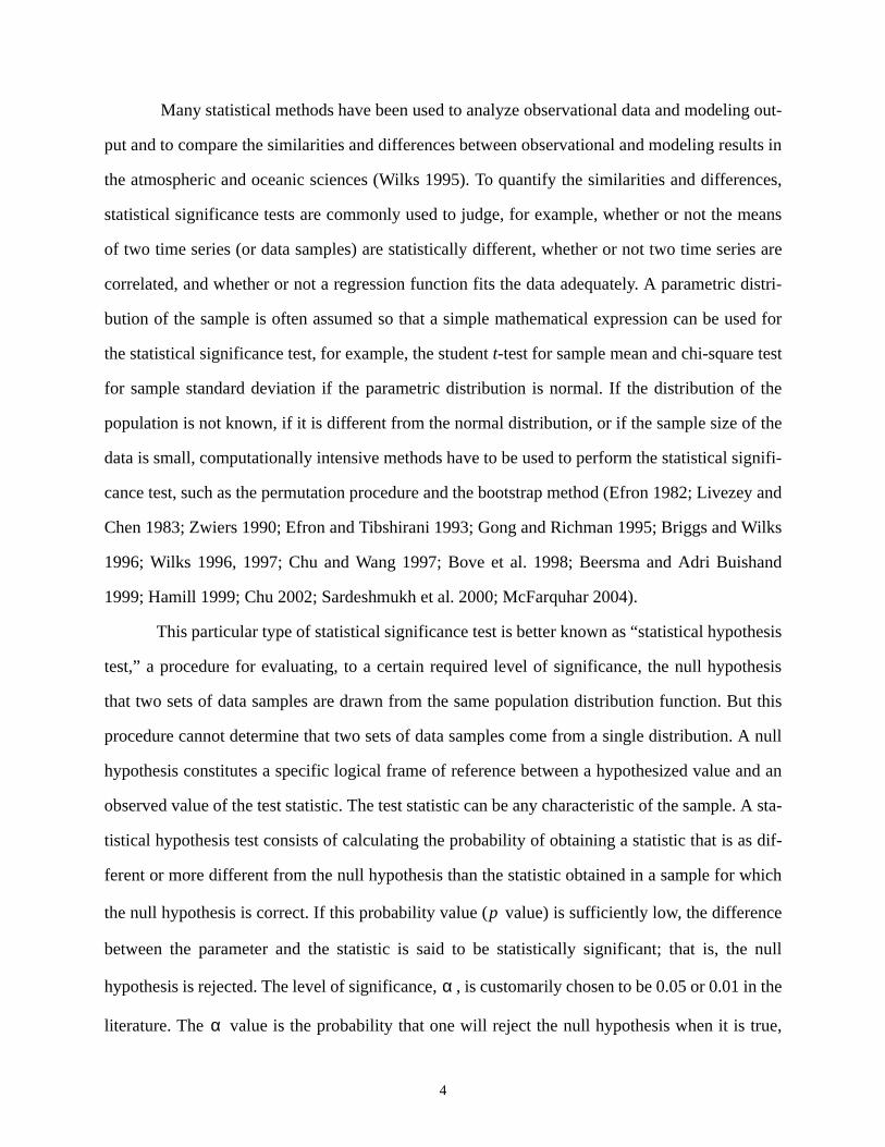
Figure 1: Histograms of (a) top-of-the-atmosphere (TOA) albedo and (b) cloud top height for

eight selected tropical convective cloud objects observed during the March 1998 period.

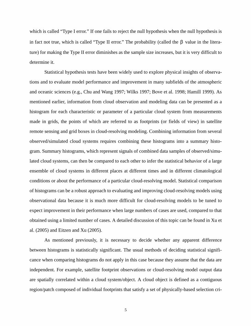
Figure 2: Observed histograms for (a) cloud optical depth, (b) outgoing longwave radiation flux,

(c) ice water path, (d) top-of-the-atmosphere albedo, (e) cloud top height and (d) sea sur-

face temperature for S (equivalent diameters of 100 - 150 km), M (equivalent diameters of

150 - 300 km) and L (equivalent diameters greater than 300 km) size categories.

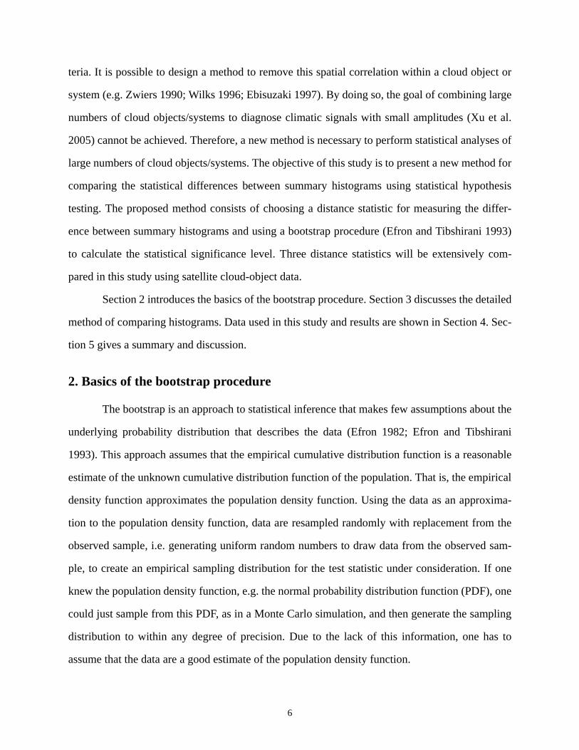
Figure 3: Empirical sampling distributions of bootstrap distances for the six parameters shown in

Fig. 2 between the S (equivalent diameters of 100-150 km) and M (equivalent diameters

of 150-300 km) size categories (solid lines), between the M and L (equivalent diameters

greater than 300 km) size categories (short dashed line) and between the S and L size cat-

egories (long dashed line) using the L2 test statistic. The bin interval is 0.004 in all panels,

except for (e), which uses a bin interval of 0.008. The vertical bars in each panel indicate

the observed L2, JM and Kp distances. Note that the axes in (f) are different from those in

the rest of the panels.

Figure 4: Same as Fig. 3 except for using the JM test statistic.

Figure 5: Same as Fig. 3 except for using the Kuiper test statistic.

23

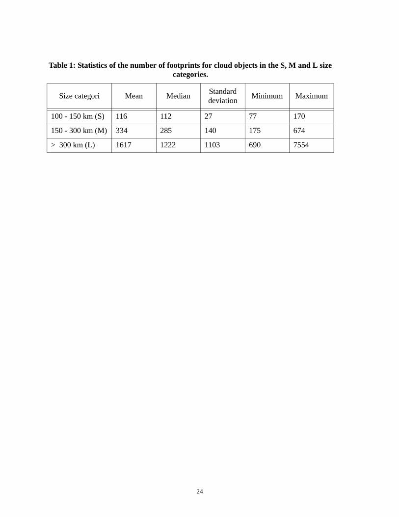
Table 1: Statistics of the number of footprints for cloud objects in the S, M and L size categories.

Size categori Mean MedianStandard deviation

Minimum Maximum

100 - 150 km (S) 116 112 27 77 170

150 - 300 km (M) 334 285 140 175 674

> 300 km (L) 1617 1222 1103 690 7554

24

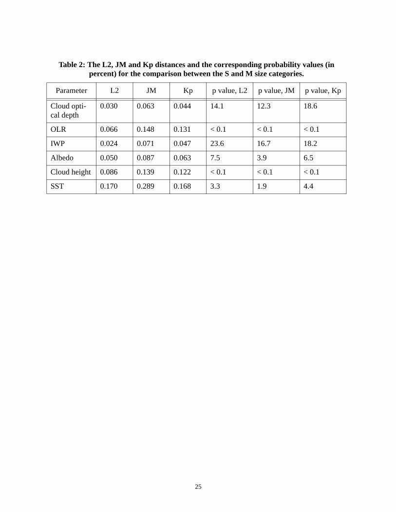
Table 2: The L2, JM and Kp distances and the corresponding probability values (in percent) for the comparison between the S and M size categories.

Parameter L2 JM Kp p value, L2 p value, JM p value, Kp

Cloud opti-cal depth

0.030 0.063 0.044 14.1 12.3 18.6

OLR 0.066 0.148 0.131 < 0.1 < 0.1 < 0.1

IWP 0.024 0.071 0.047 23.6 16.7 18.2

Albedo 0.050 0.087 0.063 7.5 3.9 6.5

Cloud height 0.086 0.139 0.122 < 0.1 < 0.1 < 0.1

SST 0.170 0.289 0.168 3.3 1.9 4.4

25

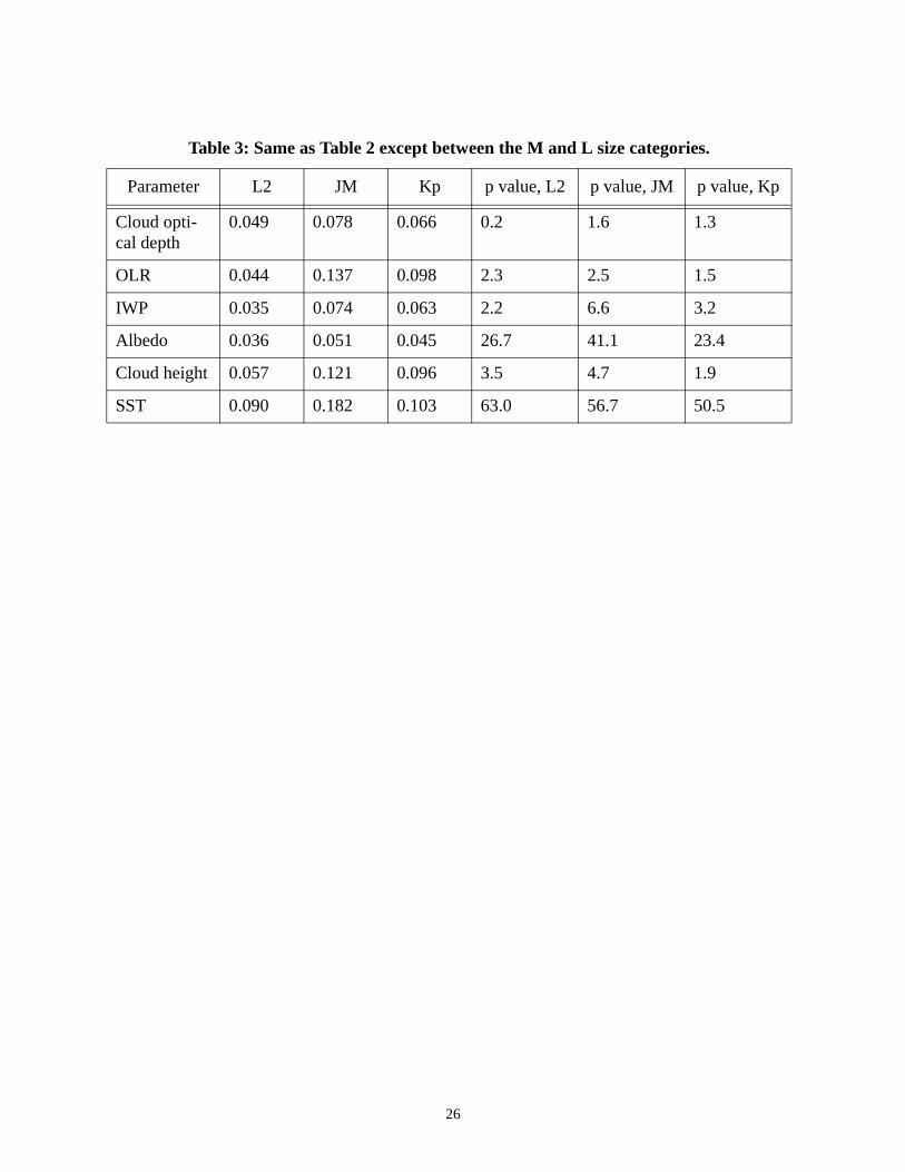
Table 3: Same as Table 2 except between the M and L size categories.

Parameter L2 JM Kp p value, L2 p value, JM p value, Kp

Cloud opti-cal depth

0.049 0.078 0.066 0.2 1.6 1.3

OLR 0.044 0.137 0.098 2.3 2.5 1.5

IWP 0.035 0.074 0.063 2.2 6.6 3.2

Albedo 0.036 0.051 0.045 26.7 41.1 23.4

Cloud height 0.057 0.121 0.096 3.5 4.7 1.9

SST 0.090 0.182 0.103 63.0 56.7 50.5

26

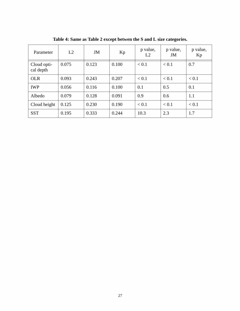
Table 4: Same as Table 2 except betwen the S and L size categories.

Parameter L2 JM Kpp value,

L2p value,

JMp value,

Kp

Cloud opti-cal depth

0.075 0.123 0.100 < 0.1 < 0.1 0.7

OLR 0.093 0.243 0.207 < 0.1 < 0.1 < 0.1

IWP 0.056 0.116 0.100 0.1 0.5 0.1

Albedo 0.079 0.128 0.091 0.9 0.6 1.1

Cloud height 0.125 0.230 0.190 < 0.1 < 0.1 < 0.1

SST 0.195 0.333 0.244 10.3 2.3 1.7

27

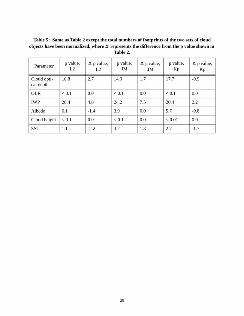
Table 5: Same as Table 2 except the total numbers of footprints of the two sets of cloud objects have been normalized, where represents the difference from the p value shown in

Table 2.

Parameterp value,

L2 p value,

L2p value,

JM p value,

JMp value,

Kp p value,

Kp

Cloud opti-cal depth

16.8 2.7 14.0 1.7 17.7 -0.9

OLR < 0.1 0.0 < 0.1 0.0 < 0.1 0.0

IWP 28.4 4.8 24.2 7.5 20.4 2.2

Albedo 6.1 -1.4 3.9 0.0 5.7 -0.8

Cloud height < 0.1 0.0 < 0.1 0.0 < 0.01 0.0

SST 1.1 -2.2 3.2 1.3 2.7 -1.7

∆

∆ ∆ ∆

28

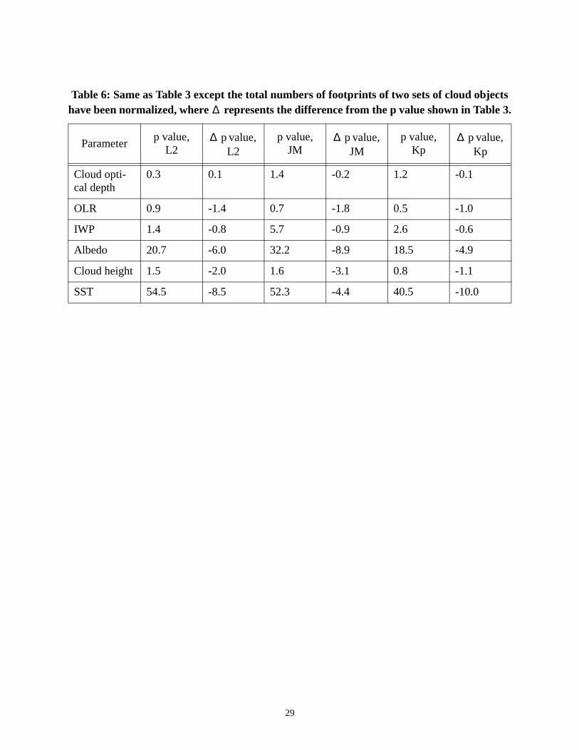
Table 6: Same as Table 3 except the total numbers of footprints of two sets of cloud objects have been normalized, where represents the difference from the p value shown in Table 3.

Parameterp value,

L2 p value,

L2p value,

JM p value,

JMp value,

Kp p value,

Kp

Cloud opti-cal depth

0.3 0.1 1.4 -0.2 1.2 -0.1

OLR 0.9 -1.4 0.7 -1.8 0.5 -1.0

IWP 1.4 -0.8 5.7 -0.9 2.6 -0.6

Albedo 20.7 -6.0 32.2 -8.9 18.5 -4.9

Cloud height 1.5 -2.0 1.6 -3.1 0.8 -1.1

SST 54.5 -8.5 52.3 -4.4 40.5 -10.0

∆

∆ ∆ ∆

29

Fig. 1: Histograms of (a) top-of-the-atmosphere (TOA) albedo and (b) cloud top height for

eight selected tropical convective cloud objects observed during the March 1998 period.

6.0

5.0

4.0

3.0

2.0

1.0

0.00.3 0.4 0.5 0.6 0.7 0.8 0.9

0.4

0.3

0.2

0.1

0.010 11 12 13 14 15 16

(a)

(b)

30

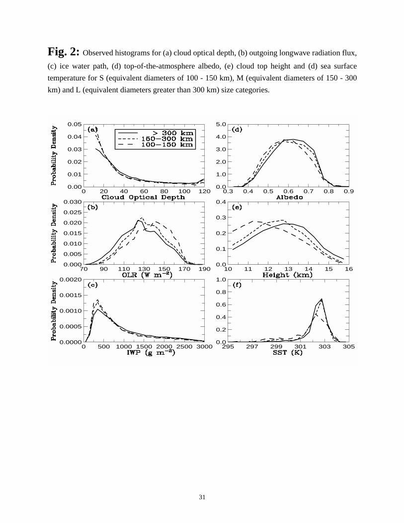
Fig. 2: Observed histograms for (a) cloud optical depth, (b) outgoing longwave radiation flux,

(c) ice water path, (d) top-of-the-atmosphere albedo, (e) cloud top height and (d) sea surface

temperature for S (equivalent diameters of 100 - 150 km), M (equivalent diameters of 150 - 300

km) and L (equivalent diameters greater than 300 km) size categories.

0.05

0.04

0.03

0.02

0.01

0.000 20 40 60 80 100 120

0.030

0.025

0.020

0.015

0.010

0.005

0.00070 90 110 130 150 170 190

0.0020

0.0015

0.0010

0.0005

0.00000 500 1000 1500 2000 2500 3000

5.0

4.0

3.0

2.0

1.0

0.00.3 0.4 0.5 0.6 0.7 0.8 0.9

0.4

0.3

0.2

0.1

0.010 11 12 13 14 15 16

1.0

0.8

0.6

0.4

0.2

0.0295 297 299 301 303 305

31

Fig. 3: Empirical sampling distributions of bootstrap distances for the six parameters shown

in Fig. 2 between the S (equivalent diameters of 100-150 km) and M (equivalent diameters of

150-300 km) size categories (solid lines), between the M and L (equivalent diameters greater than

300 km) size categories (short dashed line) and between the S and L size categories (long dashed

line) using the L2 test statistic. The bin interval is 0.004 in all panels, except for (e), which uses a

bin interval of 0.008. The vertical bars in each panel indicate the observed L2, JM and Kp

distances. Note that the axes in (f) are different from those in the rest of the panels.

0.25

0.20

0.15

0.10

0.05

0.000.00 0.05 0.10 0.15 0.20

0.25

0.20

0.15

0.10

0.05

0.000.00 0.05 0.10 0.15 0.20

0.25

0.20

0.15

0.10

0.05

0.000.00 0.05 0.10 0.15 0.20

0.25

0.20

0.15

0.10

0.05

0.000.00 0.05 0.10 0.15 0.20

0.25

0.20

0.15

0.10

0.05

0.000.00 0.05 0.10 0.15 0.20

0.15

0.12

0.09

0.06

0.03

0.000.00 0.05 0.10 0.15 0.20 0.25 0.30

32

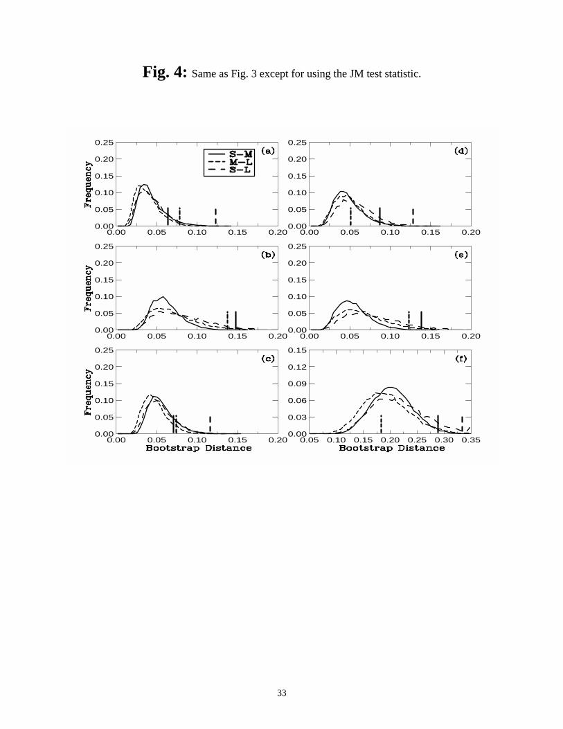
Fig. 4: Same as Fig. 3 except for using the JM test statistic.

0.25

0.20

0.15

0.10

0.05

0.000.00 0.05 0.10 0.15 0.20

0.25

0.20

0.15

0.10

0.05

0.000.00 0.05 0.10 0.15 0.20

0.25

0.20

0.15

0.10

0.05

0.000.00 0.05 0.10 0.15 0.20

0.25

0.20

0.15

0.10

0.05

0.000.00 0.05 0.10 0.15 0.20

0.25

0.20

0.15

0.10

0.05

0.000.00 0.05 0.10 0.15 0.20

0.15

0.12

0.09

0.06

0.03

0.000.05 0.10 0.15 0.20 0.25 0.30 0.35

33

Fig. 5:Same as Fig. 3 except for using the Kuiper test statistic.

0.25

0.20

0.15

0.10

0.05

0.000.00 0.05 0.10 0.15 0.20

0.25

0.20

0.15

0.10

0.05

0.000.00 0.05 0.10 0.15 0.20

0.25

0.20

0.15

0.10

0.05

0.000.00 0.05 0.10 0.15 0.20

0.25

0.20

0.15

0.10

0.05

0.000.00 0.05 0.10 0.15 0.20

0.25

0.20

0.15

0.10

0.05

0.000.00 0.05 0.10 0.15 0.20

0.15

0.12

0.09

0.06

0.03

0.000.00 0.05 0.10 0.15 0.20 0.25 0.30

34