using statistics in validation -- small molecule … · using statistics in validation -- small...
TRANSCRIPT


Jane Weitzel Biosketch
Jane Weitzel has been working in analytical chemistry for
over 35 years for mining and pharmaceutical companies with
the last 5 years at the director/associate director level. She
is currently a consultant, auditor, and trainer. Jane has
applied Quality Systems and statistical techniques, including
the estimation and use of measurement uncertainty, in a
wide variety of technical and scientific businesses. She has
obtained the American Society for Quality Certification for
both Quality Engineer and Quality Manager.
In 2014 she was pointed to the Chinese National Drug
Reference Standards Committee and attended their
inaugural meeting in Beijing
For the 2015 – 2020 cycle, Jane is a member of the USP
Statistics Expert Committee and Expert Panel on Method
Validation and Verification.

Disclaimer
This presentation reflects the speaker’s
perspective on this topic and does not
necessarily represent the views of USP or
any other organization.


Authors of the Paper
Jane Weitzel
Robert Forbes
Principal Scientist of Roche Diabetes Care
Formerly with Eli Lilly
Ron Snee
Founder and president of Snee Associates

TWO BASIC STATISTICAL
CONCEPTS
Central Limit Theorem
Confidence Interval of the Standard Deviation (SD)

Central Limit Theorem
The distribution of an average is normal.
The sampling distribution of sample means
tends to be a normal distribution.


Confidence Interval of the Standard
Deviation (SD) Each time a standard deviation is estimated,
a different value may be obtained
The confidence interval for the standard
deviation can be calculated
A range within which you expect to find the SD
with a certain level of confidence
Width of the range depends upon number of
measurements used to calculate the SD and the
confidence level you choose
Let’s look at an example

TMU and MU variability
Replicate Experiment 1 Experiment 2 Experiment 3 Experiment 4 Experiment 5 Experiment 6
1 98.81 100.68 100.51 100.53 98.74 99.15
2 99.21 100.72 100.44 99.81 99.51 100.86
3 100.41 99.17 99.58 100.47 100.38 100.04
4 99.16 99.85 99.12 99.44 100.98 101.27
5 100.90 99.46 100.84 99.49 100.43 99.28
6 99.96 100.85 99.68 99.95 100.42 99.16
7 98.93 99.34 100.65 99.94 98.85 100.18
Standard
Deviation (s) 0.81 0.72 0.65 0.43 0.87 0.85
Minimum s 0.43
Maximum s 0.87

Upper & Lower Factors
Chi Square distribution
Degrees
of
freedom
= 0.05 = 0.01 = 0.001
BU BL BU BL BU BL
1 17.79 .358 86.31 .297 844.4 .248
2 4.86 .458 10.70 .388 33.3 .329
3 3.18 .518 5.45 .445 11.6 .382
4 2.57 .519 3.89 .486 6.94 .422
5 2.25 .590 3.18 .518 5.08 .453
10 1.69 .678 2.06 .612 2.69 .549
15 1.51 .724 1.76 .663 2.14 .603
20 1.42 .754 1.61 .697 1.89 .640

Example
N=6, DF=5
SD = 0.21
Confidence Level 95% (α=0.05)
We are 95% confident that if we make another 6
measurements, the SD will be within this range
UL = 0.21 * 2.25 = 0.12
LL = 0.21 * 0.590 = 0.47

Examples with Chart
Trial Trial Std Dev Low CI High CI
1 1.64 0.97 3.70
2 2.07 1.22 4.66
3 1.03 0.61 2.31
4 1.72 1.01 3.86
5 1.58 0.93 3.55
6 2.11 1.25 4.75
7 1.57 0.92 3.52
8 1.86 1.10 4.18
9 1.53 0.91 3.45
10 2.37 1.40 5.34
0.00
1.00
2.00
3.00
4.00
5.00
6.00
1 2 3 4 5 6 7 8 9 10
Trial Std Dev
Low CI
High CI

Lifecycle Approach to Validation
Current regulatory guidance around process
validation is moving away from a simple
once-and-done validation, and toward a
continuous process verification approach, al
recent FDA method validation draft guidance
discusses lifecycle approach. FDA, Guidance for Industry Analytical Procedures and Methods
Validation for Drugs and Biologics (Rockville, MD, Draft--February 2014),
online,
www.fda.gov/downloads/drugs/guidancecomplianceregulatoryinformatio
n/guidances/ucm386366.pdf

Gage R&R
The use of traditional Gage R&R statistical
analysis and control sample charting, which
are commonly used in manufacturing process
validation and improvement, will also be
illustrated in the development of an analytical
procedure.
Method is analytical procedure (AP)


Decision Makers
The lifecycle
approach involves the
decision makers in
establishing the
intended use of the
reportable result.

Analytical Target Profile
Analytical Target Profile (ATP) [1], analogous
to the Quality Target Product Profile (QTPP)
in the ICH
ICH, Q8(R2), Pharmaceutical Development – Part
II: Pharmaceutical Development - Annex, Step 4
version (August 2009).
The ATP
defines the requirements for the result of a test method
based on the suitability for use of that result.

CQA
The test ensures that the DS is of adequate
potency, so that when used in the DP, the
patient will receive the appropriate dose of
the active ingredient.
In this way, potency is a critical quality
attribute (CQA) of the DS that is linked to a
CQA for the DP.

Example Parameters
An example of the potency test for a drug
substance (DS) with specification limits of
98.0% to 102.0%.
Assume the limits are on the as-is basis, and
no correction for water or solvents is
necessary
There are other CQA’s but this example will
focus on potency only.

Focus of This Example
Focus on the
precision and
uncertainty performance characteristics of the
potency test method
For Procedure Performance Qualification and
Verification demonstrate the
gage R&R tool, and
experimentally designed intermediate precision
studies

Acceptance Criterion for Precision
Set using a Decision Rule (DR)
DR uses acceptable probability of making a
wrong decision
Null Hypothesis
The potency of the sample is within specification
Two types of wrong decisions False Positive or Type I Error or Producer’s Risk or α
False negative or Type II Error or Manufacturer’s Risk or
β

False Positive or Type I Error or
Producer’s Risk or α A batch that has
acceptable potency
may test outside the
specification limits
False positive because
it is a positive test for
unacceptable potency
True value is 99.0%
Lower Limit 98
Nominal Concentration (Central Value) 99
Upper Limit 102
Measurement Uncertainty 1
% Below Lower Limit Total % Outside Limits % Above Upper Limit
15.87% 16.00% 0.13%
95 97 99 101 103 105
Concentration
LL
UL

False negative or Type II Error or
Manufacturer’s Risk or β A batch that does not
have acceptable
potency tests inside
the specification limits
False negative
because it is a
negative test for
unacceptable potency
True value is 97.0%
Lower Limit 98
Nominal Concentration (Central Value) 97
Upper Limit 102
Measurement Uncertainty 1
% Below Lower Limit Total % Outside Limits % Above Upper Limit
84.13% 84.13% 0.00%
95 97 99 101 103 105
Concentration
LL
UL

ATP uses
ATP uses the probability of each of these
errors to define the maximum allowed
measurement variation (uncertainty) for the
reported result.
This translates into an acceptance criterion
for the qualification of the analytical
procedure.

Decision Rule
The product will be considered compliant if
the measurement result is within the
acceptance zone.
94 96 98 100 102 104 106
Simple Decision Rule
Upper LimitLower Limit
Specification Zone
Rejection Zone Rejection ZoneAcceptance Zone

Type II error rate is negligible
Good Quality DS
Probability for either error
is caused by both
process variability and
measurement uncertainty.
Assume Type II error rate
is negligible because
Drug Substance is high
quality, few impurities at
very low concentrations.
Not Likely
Lower Limit 98
Nominal Concentration (Central Value) 97
Upper Limit 102
Measurement Uncertainty 1
% Below Lower Limit Total % Outside Limits % Above Upper Limit
84.13% 84.13% 0.00%
95 97 99 101 103 105
Concentration
LL
UL

Probability of Type I Error
Measurement Uncertainty
Probability of Type I error
comes from
measurement variation.
Measurement uncertainty
(MU)
Hence, the probability of
Type I error determines
the probability that is
acceptable.
Likely True Value In-Spec
Lower Limit 98
Nominal Concentration (Central Value) 99
Upper Limit 102
Measurement Uncertainty 1
% Below Lower Limit Total % Outside Limits % Above Upper Limit
15.87% 16.00% 0.13%
95 97 99 101 103 105
Concentration
LL
UL

Specification is Set
The specification is set by regulators, so it
cannot be adjusted.
The only parameter that can be adjusted to
meet the probability of the decision rule is the
Measurement Uncertainty.

Measurement Uncertainty
MU Definition from the VIM:
non-negative parameter characterizing the
dispersion of the quantity values being
attributed to a measurand (the quantity being
measured), based on the information used
JCGM, International vocabulary of metrology –
Basic and general concepts and associated terms
(VIM), 3rd ed., JCGM 200:2012(E/F), online,
www.bipm.org/utils/common/documents/jcgm/JC
GM_200_2012.pdf

Intermediate Precision
Test will be carried out in a single laboratory
Intermediate Precision is suitable parameter
for precision to estimate the analytical
procedure capability
Must challenge likely and appropriate analytical
procedure performance characteristics that will
impact the precision


Terminology
repeatability will be used to describe short-
term variability (i.e., repeat preparations
within a single run)
intermediate precision to describe long-term
variability within a single lab (i.e.,
preparations analyzed over different
runs/setups)
Gage R and R
Repeatability and Reproducibility

Gage R&R
Terminology associated with the use of the
Gage R&R tool does not make the distinction
between within-lab and inter-lab precision
estimates,
S in this example, the term “reproducibility”
means the same thing as “intermediate
precision.”

MU Distribution
Assume the MU distribution is normal
basis for this assumption is discussed in
Annex G of the GUM.
Even if the distribution is not normal, the same
approach will be used.
ISO/IEC, Uncertainty of measurement – Part 3:
Guide to the expression of uncertainty in
measurement (GUM:1995), 98-3:2008.
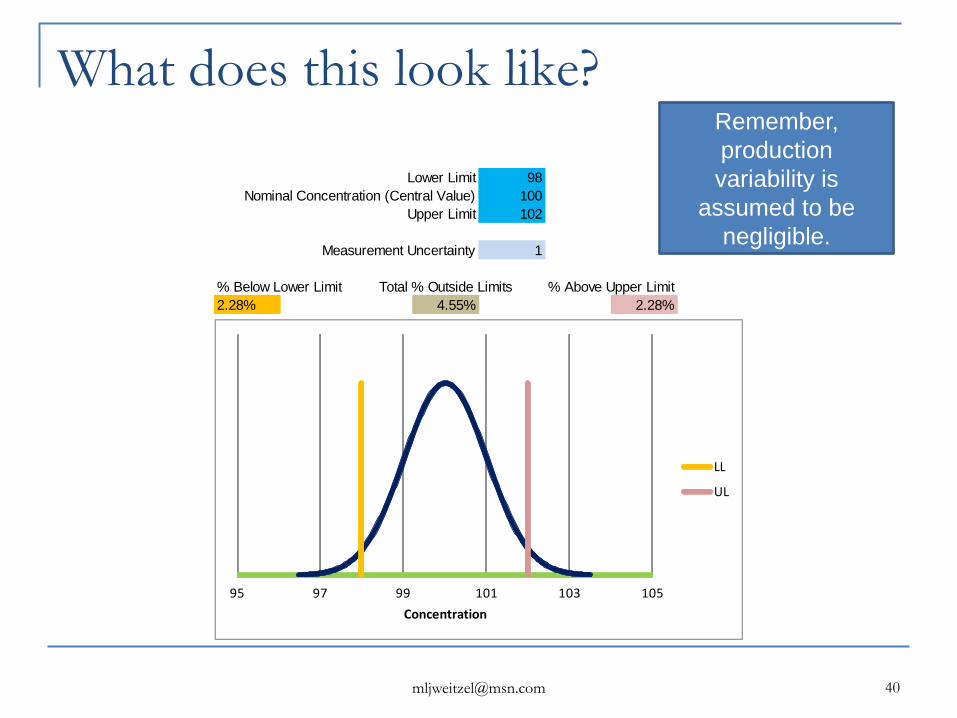
What does this look like?
Lower Limit 98
Nominal Concentration (Central Value) 100
Upper Limit 102
Measurement Uncertainty 1
% Below Lower Limit Total % Outside Limits % Above Upper Limit
2.28% 4.55% 2.28%
95 97 99 101 103 105
Concentration
LL
UL
Remember,
production
variability is
assumed to be
negligible.

MU is 1.0%, Probability is 5%
Add 5% to DR
The batch of DS will be
considered compliant if
the result is within 98.0 to
102.0%, with a 5%
probability of being
wrong.
This probability is
“theoretical” or ideal.
Simple Decision Rule
94 96 98 100 102 104 106
Simple Decision Rule
Upper LimitLower Limit
Specification Zone
Rejection Zone Rejection ZoneAcceptance Zone
MU at 1.0%
Any analytical procedure that produces
results with an MU of 1.0% or less is fit for its
intended use.
The Target Measurement Uncertainty (TMU)
is 1.0%.
TMU is defined in the VIM as the “measurement
uncertainty specified as an upper limit and
decided on the basis of the intended use of the
measurement results” VIM,http://www.bipm.org/en/publications/guides/vim.html

Analytical Target Profile
ATP can now be set.
The laboratory qualifies the analytical
procedure for a range larger than 98.0 to
102.0%.
There is only one known impurity, Impurity A,
and its concentration is <0.1%.

ATP
The analytical procedure must be able to
quantify the drug substance in the presence
of impurity A, and potential degradation
products, over a range of 80% to 120% of the
nominal concentration with an accuracy and
uncertainty so that the reportable result falls
within ±2% of the true value with at least a
95% probability.

Performance Characteristics for the
Analytical Procedure Use the ATP to define performance
characteristics for the analytical procedure
Accuracy, precision, specificity, linearity and
range
As long as their impact on the accuracy and
precision is such that the target measurement
uncertainty can be met, they are acceptable.
Advantage of this approach – you can define “Good Enough”

Acceptance Criteria
The target uncertainty is NMT 1.0%. The
combination of bias and uncertainty need to
be such that the probability of not meeting the
specification is NMT 5%.
In order to meet the ATP, the acceptance
criterion for the study is that the overall
variability, the combined uncertainty, must be
NMT 1.0% as a standard uncertainty or
standard deviation.


HPLC Technique is Used
Designed experiments
Analytical procedure is developed and
qualified
Example of intermediate precision study:

Analyst Setup Instrument Column Prepa
ration
Potency
(%)
AVG(%)
A 1 HPLC-A A 1 99.58 99.64
2 99.70
A 2 HPLC-B B 1 99.50 99.58
2 99.65
B 3 HPLC-C C 1 99.43 99.28
2 99.13
B 4 HPLC-D D 1 99.69 99.53
2 99.36
C 5 HPLC-E E 1 99.61 99.64
2 99.66
C 6 HPLC-F F 1 99.60 99.62
2 99.64
D 7 HPLC-G G 1 99.55 99.53
2 99.51
D 8 HPLC-H H 1 99.79 99.79
2 99.79
SD 0.17 0.15
80%
UCL
0.23 0.20

SD < TMU
The overall standard deviation (SD) obtained
in this study was 0.15%, with an 80% UCL of
0.20%, which met the acceptance criteria of
NMT 1.0% SD
The analytical procedure is fit for its intended
use.


Install AP in QC Laboratory
Write procedure performance qualification
protocol
From the perspective of a lifecycle approach,
a key element of the transfer activity is to
show that the precision of the method as
performed in the QCL is sufficient to meet the
required uncertainty as described in the ATP.
Precision is NMT 1.0%RSD

Use Gage R&R
Could repeat the intermediate precision
experiment
An alternative is to conduct a Gage R&R
study
Remember in Gage Repeatability a&
Reproducibility, the latter is the same as
intermediate precision

Structure of R&R
In a Gage R&R Study
5-10 samples are evaluated by
2-4 analysts (reproducibility) using
2-4 repeat tests (repeatability)
sometimes involving 2-4 test instruments
(reproducibility).
For example if 3 analysts measure each of 10
samples of a product in duplicate the study will
produce 3x10x2=60 test results.

Experimental Design
Samples from
five API batches were tested on
four setups (run) by
two analysts using
each of two instruments
each instrument used a unique column for total of two
columns
New mobile phase was prepared for each setup and each
analyst prepared a fresh set of standards for each run.
Samples were prepared and analyzed in
duplicate on each run, producing a total of 5x2x2x2 = 40
Potency(%) test results.

API Batch Analyst
HPLC/ Column Test
Potency (%)
API Batch Analyst
HPLC Column Test
Potency (%)
1 A 1 1 100.0 3 A 2 1 100.4
1 A 1 2 100.1 3 A 2 2 99.6
1 B 2 1 99.4 3 B 1 1 100.6
1 B 2 2 100.3 3 B 1 2 100.8
1 A 2 1 100.4 4 A 1 1 99.5
1 A 2 2 100.8 4 A 1 2 99.3
1 B 1 1 100.8 4 B 2 1 100.8
1 B 1 2 100.3 4 B 2 2 101.5
2 A 1 1 99.8 4 A 2 1 100.4
2 A 1 2 99.5 4 A 2 2 100.2
2 B 2 1 101.3 4 B 1 1 100.2
2 B 2 2 101.1 4 B 1 2 100.3
2 A 2 1 100.9 5 A 1 1 99.8
2 A 2 2 100.5 5 A 1 2 99.6
2 B 1 1 100.6 5 B 2 1 101.3
2 B 1 2 100.4 5 B 2 2 101.0
3 A 1 1 99.2 5 A 2 1 100.2
3 A 1 2 98.9 5 A 2 2 99.9
3 B 2 1 101.3 5 B 1 1 100.7
3 B 2 2 101.6 5 B 1 2 100.2

API Batch Analyst
HPLC/ Column Test
Potency (%)
API Batch Analyst
HPLC Column Test
Potency (%)
1 A 1 1 100.0 3 A 2 1 100.4
1 A 1 2 100.1 3 A 2 2 99.6
1 B 2 1 99.4 3 B 1 1 100.6
1 B 2 2 100.3 3 B 1 2 100.8
1 A 2 1 100.4 4 A 1 1 99.5
1 A 2 2 100.8 4 A 1 2 99.3
1 B 1 1 100.8 4 B 2 1 100.8
1 B 1 2 100.3 4 B 2 2 101.5
2 A 1 1 99.8 4 A 2 1 100.4
2 A 1 2 99.5 4 A 2 2 100.2
2 B 2 1 101.3 4 B 1 1 100.2
2 B 2 2 101.1 4 B 1 2 100.3
2 A 2 1 100.9 5 A 1 1 99.8
2 A 2 2 100.5 5 A 1 2 99.6
2 B 1 1 100.6 5 B 2 1 101.3
2 B 1 2 100.4 5 B 2 2 101.0
3 A 1 1 99.2 5 A 2 1 100.2
3 A 1 2 98.9 5 A 2 2 99.9
3 B 2 1 101.3 5 B 1 1 100.7
3 B 2 2 101.6 5 B 1 2 100.2

Data Organized by Run/Setup (1& 2)
Run/Set-up Analyst HPLC/ColumnLot/Sample
API Batch
Replicate
TestPotency(%)
1 A 1 1 1 100
1 A 1 1 2 100.1
1 A 1 2 1 99.8
1 A 1 2 2 99.5
1 A 1 3 1 99.2
1 A 1 3 2 98.9
1 A 1 4 1 99.5
1 A 1 4 2 99.3
1 A 1 5 1 99.8
1 A 1 5 2 99.6
2 B 2 1 1 99.4
2 B 2 1 2 100.3
2 B 2 2 1 101.3
2 B 2 2 2 101.1
2 B 2 3 1 101.3
2 B 2 3 2 101.6
2 B 2 4 1 100.8
2 B 2 4 2 101.5
2 B 2 5 1 101.3
2 B 2 5 2 101

Data Organized by Run/Setup (3&4)
Run/Set-up Analyst HPLC/ColumnLot/Sample
API Batch
Replicate
TestPotency(%)
3 A 2 1 1 100.4
3 A 2 1 2 100.8
3 A 2 2 1 100.9
3 A 2 2 2 100.5
3 A 2 3 1 100.4
3 A 2 3 2 99.6
3 A 2 4 1 100.4
3 A 2 4 2 100.2
3 A 2 5 1 100.2
3 A 2 5 2 99.9
4 B 1 1 1 100.8
4 B 1 1 2 100.3
4 B 1 2 1 100.6
4 B 1 2 2 100.4
4 B 1 3 1 100.6
4 B 1 3 2 100.8
4 B 1 4 1 100.2
4 B 1 4 2 100.3
4 B 1 5 1 100.7
4 B 1 5 2 100.2

Variance components analysis
Used Minitab
Estimates repeatability (within set-up
variability)
Estimates reproducibility (setup to setup
variability)
multiple analysts, instruments and columns
were used to obtain more realistic variability
estimates, and could not be separately
evaluated for statistically significant effects

Gage R &R Variance Components
results of the variance components analysis
for the potency measurements are
summarized
Source of Variation Variance % of Total Std Dev
Repeatability 0.086750 16.0 0.294534
Reproducibility 0.456167 84.0 0.675401
Total Gage R&R 0.542917 100.0 0.736829


Intermediate Precision
Reportable value is average of the two
potencies analyzed in a single setup
The standard deviation is 0.71%
With an 80%upper confidence limit of 1.16%
Acceptance criterion is NMT 1.0%
The standard deviation passes but the upper
confidence limit does not

Fail Confidence Limit Criterion
If the verification protocol utilized an
acceptance criterion of NMT 1.0% for the
80% UCL of the SD, these results would not
pass the criterion

Pool results for all the batches
Make an assumption there are no significant
differences between the batches
Support this assumption with detailed analytical
results from the supplier of the drug substance
The standard deviation becomes 0.63% with
an 80% Upper Confidence Limit of 1.03%
Rounds to 1.0% that meets the acceptance
criterion

Impact of Replication
Another way to reduce the standard deviation
is to use replication
Equation to calculate intermediate precision
SD

0.71%
√((0.675401)2/1 + (0.294534)2/(1*2)) =
0.71%
Source of Variation Variance % of Total Std Dev
Repeatability 0.086750 16.0 0.294534
Reproducibility 0.456167 84.0 0.675401
Total Gage R&R 0.542917 100.0 0.736829

Impact of Replication
Increasing number of replicates within a
run/setup has little impact
Since between setup standard deviation is
larger component of variance, replicate
between setup/runs.
Number of Setups Number of Within
Setup Replicates Method Standard Deviation
(Intermediate Precision) 1 1 0.74%
1 2 0.71%
2 1 0.52%
2 2 0.50%

Benefit of Using R&R Study
You understand the variance components
Don’t waste effort by preparing replicates at
the repeatability level (within setup/run).
Waste resources
Have a false sense of assurance that precision is
improved

Compare Validation to Transfer
Estimate of the standard deviation obtained
in the QCL (0.63%, 80% UCL = 1.0%,
pooling the batches) was larger than the
standard deviation estimate obtained during
method validation (0.15%, 80% UCL =
0.20%)
Both met acceptance criterion
May be many reasons for this difference
Analysts performing validation may have been
more experienced


EXCEL and Variance
Enter Analytical Uncertainty and Production Standard Deviaion
Lower Limit 98
Nominal Concentration (Central Value) 100 Analytical Production Pooled
Upper Limit 102 Uncertainty Std Dev Std Dev
0.5 1 1.118034
Pooled Std Dev (MU with Procction Std Dev) 1.118034
% Below Lower Limit Total % Outside Limits % Above Upper Limit
3.68% 7.36% 3.68% Impact of Combined Analytical & Production Variability
Enter values for various scenarios in the table
Analytical Production Pooled % Below % Above Total %
Uncertainty Std Dev Std Dev Limit Limit Outside
Limits
85 90 95 100 105 110 115
Concentration
LL
UL

Equation
Combine standard deviations as their
variances
sc=√(sA2 + sP
2)
Sc combined standard deviation
sA analytical measurement uncertainty
sP production standard deviation
Pooled
Std Dev
=SQRT(Y5^2+Z5^2)

Calculate Production Standard
Deviation Rearrange equation to calculate production
standard deviation
√(sc2 - sA
2) = sP

Various Measurement Capability
Recommendations The Automotive Industry Action Group
(AIAG) recommends the use of 6s in gage
R&R studies.
The variation that is due to the measuring
system, either as a percent of study variation
or as a percent of tolerance, is less than
10%. According to AIAG guidelines, this is
acceptable.

For Pharmaceutical
Such recommendations may or may not work
for pharmaceutical
With knowledge and understanding of
statistics and use of experimental designs
such as Gage R&R, we can determine the
capability of our measurement systems.

Conclusion
We can use the lifecycle approach to
analytical procedures to determine
Decision rules
TMU
ATP
We can use designs such as Gage R&R to
study our analytical procedures and
demonstrate they are fit for their intended
purpose.
