using r for introductory calculus and statisticsuser2007.org/program/presentations/kaplan.pdfusing r...

Using R for Introductory Calculus and Statistics

Daniel Kaplan

Macalester College

August 9, 2007

Slide 1/35 Daniel Kaplan Using R for Introductory Calculus and Statistics

Background

I I have been using R for 11 years for introductory statistics.I 5 years ago we started to revise our year-one introductory

curriculum: Calculus and Statistics.I Calculus and Statistics topics were entirely unrelated before

this.I Major theme of the revision was applied multivariate modeling.

This ties together the calculus and statistics closely.

I We wanted a computing platform that could support bothCalculus and Statistics.

I There is still resistence from faculty who do not appreciate thevalue of an integrated approach and who want to use apackage that they are familiar with: Mathematica, Excel,SPSS, STATA


Applied Calculus: Goals

I Intended for students who do not plan to take a multi-coursecalculus sequence.

I Give them the math they need to work in their field ofinterest, rather than the foundation for future math coursesthey will never take.


Applied Calculus: Topics

I Change: ordinary, partial, and directional derivatives.

I Optimization: including fitting and contrained optim.I Modeling:

I function building blocks: linear, polynomial, exp, sin,power-law

I functions of multiple variablesI difference & differential equations & the phase planeI units and dimensions.

I Example: polynomials to 2nd order in two variables, e.g.,bicycle speed as function of hill steepness and gear. There isan interaction between steepness and gear.


Introduction to Statistical Modeling: Goals

Give students the conceptual understanding and specific skills theyneed to address real statistical issues in their fields of interest.

I Recognize explicitly that “client” fields routinely work withmultiple variables.

I ISM provides the foundations for doing so.

I Tries to provide a unified framework that applies to manydifferent fields using different methods and terminology.

I Paradox of the conventional course:I It assumes that we need to teach students about t-tests, BUT

...I ... absurdly, that they can figure out the multivariate stuff on

their own.


Introduction to Statistical Modeling: Topics

I Linear models: interpretation of terms (incl. interactionterms), meaning of coefficients, fitting

I Issues of collinearity: Simpson’s paradox, degrees of freedom,etc.

I Basic inferential techniques:I Bootstrapping and simulation to develop conceptsI “Black box” normal theory resultsI Anova

I Theory is presented in a geometrical framework.


Who takes these courses?

I More than 100 students each year (out of a class size of 450).

I Calculus and statistics required for the biology major.

I Economics majors take it before econometrics.

I Math majors are required to take statistics (very unusual!).They take it after linear algebra.

I About 2/3 of calculus students have had some calculus inhigh school.

I About 1/3 of statistics students have had an AP-typestatistics course in high school.


What Makes R Effective?

I Free, multi-platform

I Powerful & integrated with graphics.

I Command-line based & modeling language

I Extensible, programmable

I Functional style, incl. lazy evaluation. This allows sensiblecommand-line interfaces.


Example from Calculus: FunctionsWhat students need to know about functions:

I Functions take one or more arguments and return a value.

I Definition of a function describes the rule.

I Application of a function to arguments produces the value.

R supports definition with little syntactical overhead

f = function(x){ x^2 + 2*x }

and application is very easy

> f(3)[1] 15

R emphasizes that the function itself is a thing, distinct from itsapplication:

> ffunction(x){ x^2 + 2*x }


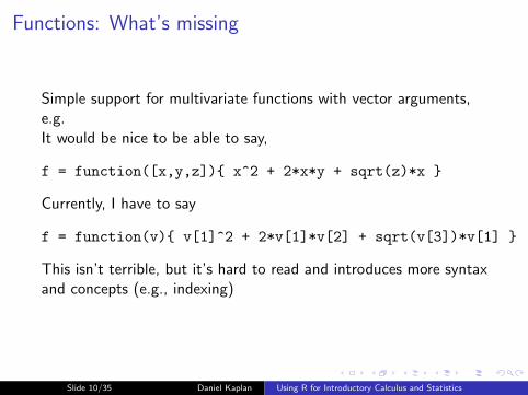
Functions: What’s missing

Simple support for multivariate functions with vector arguments,e.g.It would be nice to be able to say,

f = function([x,y,z]){ x^2 + 2*x*y + sqrt(z)*x }

Currently, I have to say

f = function(v){ v[1]^2 + 2*v[1]*v[2] + sqrt(v[3])*v[1] }

This isn’t terrible, but it’s hard to read and introduces more syntaxand concepts (e.g., indexing)


Vectors: What’s Missing?

I Simple, concise operations for assembling matrices. It’s uglyto say:

> M = cbind( rbind(1,2,3), rbind(6,5,4) )[,1] [,2]

[1,] 1 6[2,] 2 5[3,] 3 4

I Matlab-like consistency. If you extract a column from amatrix, it should be a column. NOT

> M[,1][1] 1 2 3


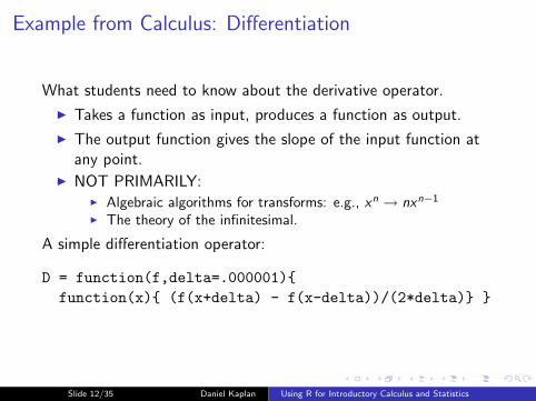
Example from Calculus: Differentiation

What students need to know about the derivative operator.

I Takes a function as input, produces a function as output.

I The output function gives the slope of the input function atany point.

I NOT PRIMARILY:I Algebraic algorithms for transforms: e.g., xn → nxn−1

I The theory of the infinitesimal.

A simple differentiation operator:

D = function(f,delta=.000001){function(x){ (f(x+delta) - f(x-delta))/(2*delta)} }


Using D> f = function(x){ x^2 + 2*x }> plot(f, 0, 10)

> plot(D(f), 0, 10)

−10 −5 0 5 10

020

6010

0

x

f (x)

Numerical pathology of (D(D(f)))> plot(D(D(f)), 0, 10)

−10 −5 0 5 10

1.99

41.

998

2.00

2

x

D(D

(f))

(x)


Using D> f = function(x){ x^2 + 2*x }> plot(f, 0, 10)> plot(D(f), 0, 10)

−10 −5 0 5 10

020

6010

0

x

f (x)

−10 −5 0 5 10

−10

010

20

x

D(f

) (x

)

Numerical pathology of (D(D(f)))> plot(D(D(f)), 0, 10)

−10 −5 0 5 10

1.99

41.

998

2.00

2

x

D(D

(f))

(x)


Using D> f = function(x){ x^2 + 2*x }> plot(f, 0, 10)> plot(D(f), 0, 10)

−10 −5 0 5 10

020

6010

0

x

f (x)

−10 −5 0 5 10

−10

010

20

x

D(f

) (x

)Numerical pathology of (D(D(f)))> plot(D(D(f)), 0, 10)

−10 −5 0 5 10

1.99

41.

998

2.00

2

x

D(D

(f))

(x)


Why not the built-in D?I It doesn’t reinforce the notion of an operator on functions.I It’s too complicated.

> g = deriv( ~ sin( 3*x), ’x’)> gexpression({

.expr1 <- 3 * x; .value <- sin(.expr1)

.grad <- array(0, c(length(.value), 1), list(NULL, c("x")))

.grad[, "x"] <- cos(.expr1) * 3; attr(.value, "gradient") <- .grad

.value})> x = 7> eval(g)[1] 0.8366556attr(,"gradient")

x[1,] -1.643188

I need to understand better the relationship between functions andformulas, and operations on formulas for extracting structure.


Example: Fitting Linear Models

R makes this amazingly easy.

> g = read.csv(’galton-heights.csv’)family father mother sex height nkids

1 1 78.5 67.0 M 73.2 42 1 78.5 67.0 F 69.0 4...6 2 75.5 66.5 M 72.5 4and so on

> lm( height ~ sex + father, data=g)(Intercept) sexM father

34.4611 5.1760 0.4278> lm( height ~ sex + father + mother, data=g)(Intercept) sexM father mother

15.3448 5.2260 0.4060 0.3215


Operating on the results of linear modeling

Sum of squares relationship:

> sum( g$height^2)[1] 4013892> m1 = lm( height ~ sex + father, data=g)> sum( m1$fitted^2) + sum( m1$resid^2)[1] 4013892> m2 = lm( height ~ sex + father + mother, data=g)> sum( m2$fitted^2) + sum( m2$resid^2)[1] 4013892

Orthogonality of fitted and residual

> sum( m2$fitted * m2$resid )[1] 4.239498e-12 -- essentially 0


Modeling: What’s missing

Syntax is not forgiving of small mistakes:

I Mis-spelled column name:

> sum( g$heights )[1] 0> sum( g$height )[1] 59951.1

I Named argument confounding. You flip 50 fair coins. Where’sthe 10th percentile on the number of heads?

> qbinom( .10, size=50, prob=.5)[1] 20> qbinom( .10, size=50, p=.5)[1] 5


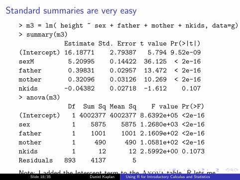
Standard summaries are very easy

> m3 = lm( height ~ sex + father + mother + nkids, data=g)> summary(m3)

Estimate Std. Error t value Pr(>|t|)(Intercept) 16.18771 2.79387 5.794 9.52e-09sexM 5.20995 0.14422 36.125 < 2e-16father 0.39831 0.02957 13.472 < 2e-16mother 0.32096 0.03126 10.269 < 2e-16nkids -0.04382 0.02718 -1.612 0.107> anova(m3)

Df Sum Sq Mean Sq F value Pr(>F)(Intercept) 1 4002377 4002377 8.6392e+05 <2e-16sex 1 5875 5875 1.2680e+03 <2e-16father 1 1001 1001 2.1609e+02 <2e-16mother 1 490 490 1.0581e+02 <2e-16nkids 1 12 12 2.5992e+00 0.1073Residuals 893 4137 5

Note: I added the Intercept term to the Anova table. R lets medo this.


Extensibility is important to teaching

Example 1: the t-test, Anova, and regression.I want to show these are different aspects of the same thing.

> t.test(g$height)t = 558.37, df = 897, p-value < 2.2e-16> summary( lm( height ~ 1, data=g ) )

Estimate Std. Error t value Pr(>|t|)(Intercept) 66.7607 0.1196 558.4 <2e-16> anova( lm( height ~ 1, data=g ) )

Df Sum Sq Mean Sq F value Pr(>F)(Intercept) 1 4002377 4002377 311777 < 2.2e-16Residuals 897 11515 13> sqrt(311777)[1] 558.37


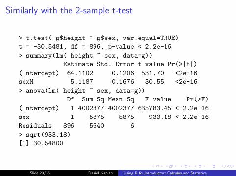
Similarly with the 2-sample t-test

> t.test( g$height ~ g$sex, var.equal=TRUE)t = -30.5481, df = 896, p-value < 2.2e-16> summary(lm( height ~ sex, data=g))

Estimate Std. Error t value Pr(>|t|)(Intercept) 64.1102 0.1206 531.70 <2e-16sexM 5.1187 0.1676 30.55 <2e-16> anova(lm( height ~ sex, data=g))

Df Sum Sq Mean Sq F value Pr(>F)(Intercept) 1 4002377 4002377 635783.45 < 2.2e-16sex 1 5875 5875 933.18 < 2.2e-16Residuals 896 5640 6> sqrt(933.18)[1] 30.54800


Extensibility is important: Example 2

How Anova Works.Let’s add k random, junky terms to a model and see how R2 orthe fitted sum of squares changes.rand(k) notation added to modeling language.

Model R2 ∆R2

footwidth~1+sex+footlength 0.4596footwidth~1+sex+footlength+rand(1) 0.4824 0.02284footwidth~1+sex+footlength+rand(2) 0.4911 0.00873footwidth~1+sex+footlength+rand(3) 0.4941 0.00297

... and so on ...footwidth~1+sex+footlength+rand(34) 0.9676 0.00365footwidth~1+sex+footlength+rand(35) 0.9820 0.01440footwidth~1+sex+footlength+rand(36) 1.0000 0.01799footwidth~1+sex+footlength+rand(37) 1.0000 0.00000footwidth~1+sex+footlength+rand(38) 1.0000 0.00000


The Modeling WalkA model with 3 model terms fit to data with 39 cases.

0.0

0.2

0.4

0.6

0.8

1.0

R^2 versus m

m (number of explanatory vectors in model)

R2

1 4 39

m=

39 T

erm

s fit

the

N=

39 c

ases

per

fect

ly

x

x

x●

● ● ● ●

● ● ● ● ●●

● ●

●● ● ● ●

●●

● ● ●

● ● ● ●

●●

● ● ●

● ●●

● ● ● ● ● ● ● ●

Inte

rcep

tse

xfo

otle

ngth

Random Terms


Resampling

Resampling itself is a conceptually simple operation.

> resample( c(1,2,3), 10)[1] 1 3 1 1 3 3 3 1 1 2

> resample( g, 5)family father mother sex height nkids

282 70 70.0 65.0 F 62.5 574 20 72.7 69.0 F 66.0 8149 40 71.0 66.0 M 71.0 5282.1 70 70.0 65.0 F 62.5 561 17 73.0 64.5 F 66.5 6


Repetition is conceptually simple, but ...

... generally hard for neophytes to implement on the computer.Not in R!Example: Roll three dice and add them.

> sum( resample( 1:6, 3) )[1] 8

Now do this 50 times:

> repeattrials( sum( resample( 1:6, 3) ), 50 )[1] 14 6 12 10 7 13 13 11 13 10 11 6 7 5 16 14 11 13

[19] 16 7 7 9 6 10 8 10 7 15 10 14 12 14 8 11 4 10[37] 14 10 12 10 8 12 12 8 7 4 17 16 10 11


Bootstrapping

Bootstrapping is hardly ever done in introductory statistics courses,even though it is so simple conceptually. This is because there islittle computational support beyond the black-box type.

> mean( resample( g$height ) )[1] 66.64577> mean( resample( g$height ) )[1] 66.76303> s = repeattrials(mean( resample( g$height ) ), 500 )

> hist(s)> quantile( s, c(0.025, 0.975) )

2.5% 97.5%66.52771 66.97620

Histogram of s

sF

requ

ency

66.4 66.6 66.8 67.0 67.2

050

100

150


A command-line interface has big advantagesIt allows us to put things together in creative ways.Example 1: Confidence intervals on model coefficients.

> lm( height ~ sex + nkids, data=g )(Intercept) sexM nkids

64.8013 5.0815 -0.1095> lm( height ~ sex + nkids, data=resample(g) )(Intercept) sexM nkids

64.73765 5.15831 -0.09852> s = repeattrials(lm( height ~ sex + nkids,

data=resample(g) )$coef, 1000)> head(s)(Intercept) sexM nkids

1 65.01683 5.323394 -0.16646742 64.64250 5.262300 -0.10054913 64.75436 5.113593 -0.1079453and so on

> quantile( s$nkids, c(0.025, 0.975))2.5% 97.5%

-0.16115645 -0.03391969


Resampling: Example 2Hypothesis testing on single variables:

> lm( height ~ sex + nkids, data=g )(Intercept) sexM nkids

64.8013 5.0815 -0.1095> lm( height ~ sex + resample(nkids), data=g )

(Intercept) sexM resample(nkids)64.00688 5.12503 0.01628

> s = repeattrials(lm( height ~ sex + resample(nkids),data=g )$coef, 1000)

> head(s)(Intercept) sexM resample(nkids)

1 63.99812 5.117672 0.018211682 64.18064 5.119589 -0.01154208

and so on> quantile( s[,3], c(0.025, 0.975))

2.5% 97.5%-0.05690810 0.05361429

Our observed value of −0.1095 is outside of this range.Slide 27/35 Daniel Kaplan Using R for Introductory Calculus and Statistics

Resampling: Example 3Power/Sample-size demonstration. If the world were like oursample, how likely is a sample of 100 people to demonstrate thatfamily size (nkids) is related to height?

# Extract the p-value on nkids> anova( lm(height ~ sex + nkids, data=g))[3,5][1] 0.0004454307# Simulate a sample of size 100> anova( lm(height ~ sex + nkids, data=resample(g,100)))[3,5][1] 0.2743715> s = repeattrials(anova( lm(height ~ sex + nkids, data=resample(g,100)))[3,5], 1000)> head(s)[1] 0.001870581 0.498089249 0.801042654 0.286201801[5] 0.055200572 0.198855304 and so on> table( s < .05 )FALSE TRUE

774 226 # power is 23%


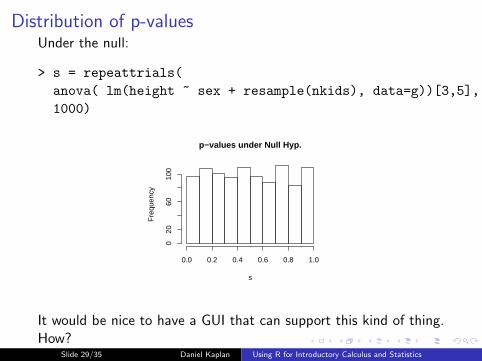
Distribution of p-valuesUnder the null:

> s = repeattrials(anova( lm(height ~ sex + resample(nkids), data=g))[3,5],1000)

p−values under Null Hyp.

s

Fre

quen

cy

0.0 0.2 0.4 0.6 0.8 1.0

020

6010

0

It would be nice to have a GUI that can support this kind of thing.How?


GUIs are Important

Examples from our courses:

I Euler method of integration.

I Visualizing dynamics on the phase plane.

I Linear combinations of vectors.

future simulating causal networks.


A graphical approach to integration

The logistic-growthsystem:x = rx(1− x/K )

I The differentialequation describeslocal dynamics.

I Growth ratechanges with x .

I Accumulate smallincrements.


0 500 1000 1500 2000

050

010

0015

0020

00

●

●

It’s also calculus to teach thephenomenology of differentialequations:

I equilibrium and stability

I oscillation

Computers can solve the DEs,so solution techniques are nolonger central.


Fitting Linear Models

A B C

3 -3 22 4 0

Fit the model A ~ B + C - 1


Local Requirements for Adopting R

I A locally accessible expert.

I Concise instructions on how to do basic things. Like KermitSigmon’s Matlab Primer.

I Things are vastly better than they once were, but still wedon’t exploit the 80/20 rule:20% of the knowledge will get you 80% of the way there!


Summary

I GUIs are important, but ...

I We should embrace R’s strength, an extensible command-lineinterface and syntax.


using r for introductory calculus and statisticsuser2007.org/program/presentations/kaplan.pdfusing r...

Documents