USING MEAN REVERSION AS A MEASURE OF PERSISTENCE∗

Daniel Dias

(Banco de Portugal)

Carlos Robalo Marques

(Banco de Portugal)

(This version: November 11, 2004)

Abstract

This paper elaborates on the alternative measure of persistence recently suggested in

Marques (2004), which is based on the idea of mean reversion. A formal distinction

between γ , the unconditional probability of a given process not crossing its mean in

period t and $γ , its estimator, is made clear and the relationship between γ and , the

widely used “sum of the autoregressive coefficients”, as alternative measures of

persistence, is investigated. Using the law of large numbers and the central limit theorem,

properties of

ρ

$γ are established, which allow tests of hypotheses on γ to be performed,

under very general conditions. Finally, some Monte Carlo experiments are conducted in

order to compare the finite sample properties of $γ and $ρ , the OLS estimator of ρ .

JEL Classification: E31, C22, E52;

Keywords: Inflation persistence; mean reversion, non-parametric estimator;

∗ We especially thank, without implicating, José Maria Brandão de Brito, José Ferreira Machado

and João Santos Silva for very useful suggestions. Helpful discussions from IPN (Inflation Persistence Network) members are also acknowledged. The usual disclaimer applies.

1

1. INTRODUCTION

Quantifying the response of inflation to shocks hitting the economy is crucial for the

implementation of monetary policy. In particular, quantifying the sluggish response of

inflation to changes in monetary conditions appears as a fundamental prerequisite if

central banks aim at implementing a pre-emptive monetary policy strategy. By

definition, however, measuring the response of inflation to shocks implies evaluating

persistence of inflation.

This paper is a contribution to a recently growing literature trying to measure

persistence of inflation. Recently Marques (2004) suggested a non-parametric

measure of persistence, which relies on the idea that there is a relationship between

persistence and mean reversion. This paper goes a step further in the direction of

establishing the properties of the estimator of such alternative measure of persistence,

which has the advantage of not requiring the specification and estimation of a model

for the series under investigation. The distinction between the theoretical concept of

mean reversion, denoted in the paper by γ and its estimator, $γ , is now made clear.

Some important theoretical properties of the estimator $γ , including unbiasedness,

consistency and its asymptotic distribution are discussed, under very general

conditions. The relationship between the different measures of persistence, with

special focus on γ and ρ , the widely used “sum of the autoregressive coefficients” is

investigated. Finally, Monte Carlo simulations are used to investigate the finite

sample properties of $γ including its robustness against outliers and potential model

misspecifications, vis-à-vis the OLS estimator of ρ .

A set of relevant results emerges from the paper. First, the process of obtaining the

theoretical value of γ for a general data generating process (DGP) is derived, and the

values of γ for a set of AR(1) and AR(2) models are specifically presented, where γ

is the unconditional probability of a given process not crossing its mean in period t.

Second, we analyse the distributional properties of $γ for a very broad class of

stationary processes. In particular, when the mean of the time series process is known,

we show that $γ is an unbiased estimator of γ . When the mean is unknown, we use the

law of large numbers to show that $γ is a consistent estimator of γ . Finally, using the

2

central limit theorem, we demonstrate that $γ has an asymptotic normal distribution, so

that tests of hypotheses on γ can be performed. The implementation of such tests

requires an estimate of the spectral density at frequency zero, which may be obtained

using, for instance, kernel-based methods.

$

Third, using Monte Carlo simulations for the AR(1) and AR(2) processes with normal

innovations, it is confirmed that i) $γ is an unbiased estimator of γ when the mean of

the process is known and slightly downward biased when the mean of the series is

unknown; ii) as expected, the OLS estimator of ρ , $ρ , is slightly downward biased

when the mean is known and significantly downward biased when the mean is

unknown; iii) Both $γ and ρ are consistent estimators, but the biases of $ $γ are smaller

than those of ρ for any sample size; iv) the finite sample distribution of $ $γ is well

approximated by the normal distribution while that of $ρ is not; v) $ρ may be subject to

significant biases coming from the presence of additive outliers in the data or from

model misspecifications, but γ is almost not affected by the first potential source of

bias and is, by definition, totally immune to the second.

Finally, it is shown that there is a monotonic relationship between ρ and γ (and some

other measures of persistence) when the data are generated by an AR(1) process, but

such a monotonic relationship ceases to exist once higher order autoregressive

processes are considered. Assuming an AR(2) process with a fixed ρ it is shown that

just by choosing alternative combinations of the two coefficients it is possible to make

an whole set of alternative measures of persistence (including γ , the half-life, the

largest autoregressive root or the number of periods required for 99 percent of the

total adjustment to take place) to go through a wide range of variation and in opposite

directions. From this evidence it is argued that we should not stick to a single scalar

measure to evaluate persistence in higher order processes and, in particular, given

their different information content and the robustness of $γ , that ρ and γ should be

computed as companion measures of persistence, on a regular basis, in empirical

applications.

The rest of the paper is organized as follows. Section 2 briefly reviews the measures

of persistence of common use in the literature. Section 3 explains the meaning of γ

and its estimator $γ and derives the properties of $γ including its asymptotic

distribution. Section 4 discusses the relationship among alternative measures of

3

persistence in the context of the AR(1) and AR(2) models. Section 5, using Monte

Carlo simulations, investigates the finite sample properties of $γ and ρ including the

robustness of these two estimators against outliers and model misspecifications.

Section 6 concludes.

$

t

2. EXISTING MEASURES OF PERSISTENCE

This section presents a formal definition of persistence and discusses the pros and

cons of existing scalar measures of persistence1. In general terms, persistence of

inflation may be defined as the tendency of inflation to revert slowly to its equilibrium

or long run level after a shock. Usually, in order to get an estimate for the degree of

persistence, i.e., the speed with which inflation converges to its long run level after a

shock, an econometric model is specified and estimated. For instance, under the so-

called univariate approach, persistence is investigated by looking at the univariate

time series representation of inflation. For that purpose it is usually assumed that

inflation follows a stationary autoregressive process of order p (AR(p)), which may be

written as

y yt j tj

j t

p

= + +−=∑α β

1

ε (2.1)

and reparameterised as:

∆ ∆y y yt j t j tj

p

= + + − +− −=

−

∑α δ ρ( )1 11

1

ε

β

(2.2)

where

ρ ==∑ jj

p

1

(2.3)

δ ji j

β i

p

= −= +∑

1

(2.4)

In the context of model (2.1) inflation is said to be (highly) persistent if, following a

shock to the disturbance term, inflation converges slowly to its mean (which in the

context of such model is seen as representing the equilibrium level of inflation). Thus,

1 This section draws heavily on Marques (2004),

4

in the context of this parametric representation of inflation, the concept of persistence

appears as intimately linked to the impulse response function (IRF) of the AR(p)

process. However, as the impulse response function is an infinite-length vector it is

not a useful measure of persistence. To overcome such difficulty, several scalar

measures of persistence have been proposed in the literature. These include the “sum

of the autoregressive coefficients”, the “spectrum at zero frequency”, the “largest

autoregressive root” and the “half-life”.

Andrews and Chen (1994) argue that the cumulative impulse response (CIR) is

generally a good way of summarizing the information contained in the impulse

response function (IRF) and as such a good scalar measure of persistence. In a simple

AR(p) process, the cumulative impulse response is simply given by CIR

where ρ is the “sum of the autoregressive coefficients”, as defined in (2.3). As there is

a monotonic relation between the CIR and

=−1

1 ρ

ρ it follows that, under the above

assumption, one can simply rely on the “sum of the autoregressive coefficients” as a

measure of persistence.

Using the CIR=1/(1-ρ ) or simply ρ as a measure of persistence amounts to measuring

persistence as the sum of the disequilibria (deviations from equilibrium) generated

during the whole convergence period (which is infinite in the AR(p) model). The

larger the ρ , the larger the cumulative impact of the shock will be (for the full

convergence period). In the context of a simple AR(1) model, with the exception of

the half-life, as we shall see below, the different scalar measures of persistence

basically deliver the same message in relative terms. This is due to the fact that the

speed of convergence as measured in the IRF by ρ k as k →∞ is constant throughout

the whole convergence period (or, in other words, the disequilibrium in period k, ρ ,

is a fixed proportion, ρ , of the disequilibrium in period k

k

−1, ρk−1 ).

However, using ρ as a measure of persistence when the series follows an AR(p)

process with p>1 may, in some circumstances, be very misleading. Andrews and Chen

(1994) discuss several situations in which the CIR and thus also ρ might not be

sufficient to fully capture the existence of different shapes in the impulse response

function. In particular, ρ , as a measure of persistence, will not be able to distinguish

between two series in which one exhibits a large initial increase and then a subsequent

5

quick decrease in the IRF while the other exhibits a relatively small initial increase

followed by a subsequent slow decrease in the IRF. We shall show below that ρ is

also not able to distinguish between two series in which one exhibits a cyclical

behaviour while the other does not. Unfortunately, as we shall illustrate in the context

of the AR(2) process, those situations rather than being pathological are very frequent

in the context of higher order processes. For such processes the speed of convergence

may vary significantly during the convergence period and as this impacts differently

on the alternative measures of persistence the monotonic relation among such

measures which stands for the AR(1) model ceases to exist for higher order process.

( )

2σρε

σ

The “spectrum at zero frequency”, is a well-known measure of the low-frequency

autocovariance of the series and, for the AR(p) process it is given by h(

where

)01 2=−

σ ε stands for the variance of 2 ε t . Again, for a fixed σε2, there is a simple

correspondence between this concept, the CIR and ρ , and so they can be seen as

equivalent measures of persistence. However the two measures can deliver different

results if one wants to test for changes in persistence over time. In such a situation the

use of the “spectrum at zero frequency” may become problematic because changes in

persistence will be brought about not only by changes in ρ but also by changes in ε .

An additional advantage of ρ over h( as a measure of persistence is that it is more

intuitive and has a small and clearly defined range of potential variation (for a

stationary process it varies between –1 and 1), which is not the case of the “spectrum

at frequency zero”.

2

)0

The “largest autoregressive root” of model (2.1) has also been used in the literature as

a measure of persistence (see, for instance Stock, 2001). The use of this statistic as a

measure of persistence is criticised both in Andrews and Chen (1994) and in Pivetta

and Reis (2001). The main point against this statistic is that it is a very poor summary

measure of the IRF because the shape of this function depends also on the other roots

and not only on the largest one. On the positive side, an important argument favouring

the use of the largest autoregressive root as a measure of persistence is the fact that an

asymptotic theory has been developed and appropriate software is available so that it

becomes ease to compute asymptotically valid confidence intervals for the

corresponding estimates (see, Stock, 1991 and 2001).

6

Finally, the “half-life” is defined as the number of periods for which the effect of a

unit shock to inflation remains above 0.5. In the case of an AR(1) process given by

ty yt t= +−ρ ε1 it is easy to show that the half-life may be computed as h =ln( / )ln( )

1 2ρ

.

The use of the “half-life” has been criticised on several grounds (see, for instance

Pivetta and Reis, 2001). First, if the IRF is oscillating the half-life can understate the

persistence of the process. Second, even for monotonically decaying processes this

measure will not be adequate to compare two different series if one exhibits a faster

initial decrease and then a subsequent slower decrease in the IRF than the other.

Third, it may also be argued that for highly persistent processes the half-life is always

very large and thus makes it difficult to distinguish changes in persistence over time.

On the positive side, the half-life has the attractive feature that persistence is

measured in units of time, which is not the case of any of the other three above

mentioned measures of inflation persistence, and thus may be preferable for

communication purposes. This probably explains why, despite the above criticisms, it

still remains the most popular measure in the literature that investigates the

persistence of deviations from the “purchasing power parity equilibrium”.

For the AR(p) process the exact computation of the “half-life” is more complex and

for this reason, the simple expression above is usually used as an approximation to the

true half-life. However Murray and Papell (2002) argue that this expression might not

be a good approximation to the true “half-life” if the effect of the shock does not

converge to zero monotonically. For that reason below we choose to compute the

half-life directly from the IRF.

Below, we shall also use as an alternative measure of persistence “the number of time

periods required for a given proportion of the total disequilibria to accumulate”, which

appears as especially suited to evaluate how fast the series “approaches” the

equilibrium. Thus, such a measure allows discriminating between two series with the

same ρ but with different patterns of shock absorption. Specifically we shall compute

the number of time periods required for fifty, ninety five and ninety nine percent of

the total disequilibria to accumulate, denoted m50, m95, and m99, respectively2.

2 The statistics m50 , m95 and m99 are often used in the empirical econometric literature to

measure the speed of adjustment of a given endogenous variable to shocks in the exogenous variables of the model.

7

The next section discusses the alternative measure of persistence recently suggested in

Marques (2004) and establishes its main properties.

3. AN ALTERNATIVE MEASURE OF PERSISTENCE

Marques (2004) has recently suggested an alternative measure of persistence which

explores the relationship between persistence and the degree of mean reversion. In

particular, Marques (2004) suggested using the statistic

$γ = −1 nT

(3.1)

to measure the absence of mean reversion of a given series, where n stands for the

number of times the series crosses the mean during a time interval with T+1

observations.

Marques (2004) does not distinguish between the theoretical concept of mean

reversion and the corresponding estimator. However, as we shall see below this

distinction is important. Thus, we now define γ as the unconditional probability of a

given process not crossing its mean in period t, or equivalently as 1 minus the

probability of mean reversion of the process. In this context $γ as given in (3.1), whose

properties are examined in this paper, appears as a natural estimator of γ .

Even though Marques (2004) has motivated γ in the context of the AR(p) process,

after noting the relationship between ρ and the degree of mean reversion in a

stationary process, the fact is that the use of γ as a measure of persistence can be

motivated in a more general framework, independently of ρ , i.e., without the need of

any assumption about the data generating process.

In fact, the use of γ as a measure of persistence follows quite naturally from the very

definition of persistence. If a persistent series is the one which converges slowly to its

equilibrium level (i.e., the mean) after a shock, then such a series, by definition, must

exhibit a low level of mean reversion, i.e., must cross its mean only infrequently.

Similarly a non-persistent series must revert to the mean very frequently. And γ

simply measures how frequently a given time series reverts to its mean. From an

economic and political point of view it is obviously important for the central bank to

know how frequently inflation reverts to the mean, i.e., the inflation target.

8

We note that γ , by definition, and $γ , by construction, are always between zero and

one. Moreover, in Marques (2004) it is shown that for a symmetric zero mean white

noise process E , so that values of γ close to 0.5 signal the absence of any

significant persistence (white noise behaviour) while figures significantly above 0.5

signal significant persistence. On the other hand, figures below 0.5 signal negative

long-run autocorrelation.

$ .γ γ= = 0 5

It is also shown in Marques (2004) that under the assumption of a symmetric white

noise process for inflation (zero persistence) the following result holds:

$ .. /

& ( ; )γ −∩

0 50 5

0 1T

N (3.2)

Equation (3.2) allows us to carry out some simple tests on the statistical significance

of the estimated persistence (i.e., γ =0.5). However (3.2) is obtained under the

assumption of a pure white noise process and thus if the null of γ =0.5 is rejected, we

should expect $γ to have a more complicated distribution, which, in particular, may

depend on the characteristics of the data generating process.

An additional interesting property of $γ is that there is a simple relation between the

estimate of γ for a given period with T+1 observations and the estimated γ ’s for two

non-overlapping consecutive sub-periods with T +1 and T +1 observations such that

T+1= (T +1)+(T +1). In fact we have 1 2

1 2

1 11 2

1 2

1

1

1

1 2

2

2

2

1 21 2− = ≈

++

=+

++

= − + − −$ ( $ ) ( )( $ )γ αnT

n nT T

nT

TT T

nT

TT T

1 1γ α γ

or simply

$ $ ( ) $γ αγ α γ≈ + −1 1 2 (3.3)

so that persistence for the whole period is (approximately) a weighted average of the

persistence for the two consecutive periods.

In contrast to ρ which requires the data generating process (DGP) to follow a pure

autoregressive process, γ is defined independently of the specific underlying DGP. In

this sense γ as a measure of persistence is broader in scope than ρ . To see that let us

take the simplest case of an Arma(1,1) process:

y yt t t= t+ +− −ρ ε θε1 1 (3.4)

9

In model (3.4) the parameter ρ (the sum of autoregressive coefficients) is no longer

the parameter of interest as it ceases to measure persistence of the y seriest3. In fact,

we have seen that ρ is used as a measure of persistence in the context of the pure

autoregressive model because it displays a monotonic relation with the CIR of the

model. However, for model (3.4) we have CIR = + −( ) / (1 1 )θ ρ so that the one-to-one

relationship between ρ and the CIR is lost. The solution, in empirical terms, implies

using a finite order autoregressive process to approximate the true Arma model, but

this is likely to introduce additional biases into the analysis, especially if the

approximation is not good. In strong contrast, γ as a measure of persistence, is

defined irrespective of the underlying DGP. Moreover, this nice property translates to

its estimator, $γ . The estimator $γ has also the advantage of not requiring the researcher

to specify and estimate a model for the inflation process. For this reason it can be

expected to be robust against potential model misspecifications and given its non-

parametric nature also against outliers in the data. We shall investigate such a claim

below in section 5.

We now investigate the asymptotic distribution of the $γ statistic. In order to introduce

the discussion let us assume that we have a sample of data with T+1 observations,

denoted as y , ,... , generated by a stationary and ergodic process with a known

mean, µ .

0 y1 yT

The estimator of γ is computed as $ /γ = −1 n T where n is the number of times the

series, , crosses the mean during the sample period. A useful way to proceed is to

think of

yt

$γ as being equal to one minus x, where x is the sample mean of a series x

(t=1, 2, ...T) that equals 1 if the series y crosses the mean and zero otherwise. From

here it follows that all the results available in the literature concerning consistence and

asymptotic distribution of the sample mean of x apply directly to the

t

t

t $γ statistic. In

particular we can invoke the law of large numbers (LLN) and the central limit

theorem (CLT).

As a first step, we can start by noticing that x can be seen as a binomial random

variable, which equals one with probability (1-

t

γ ) and zero with probability γ . Of

3 Note the contrast with the unit root literature where the parameter ρ is the parameter of

interest no matter whether the data is generated by a pure autoregressive or by an Arma process.

10

course, in general, x is not independent of x , etc, but the structure of time

dependency is determined by the autocorrelation structure of the assumed underlying

stationary and ergodic process for y . It is possible to show that if y is a stationary

and ergodic process then x is also a stationary and ergodic process because it is a

measurable function of the current and past values of y

t xt t− −1 2, ,...

t

t t

t

4. Thus it follows from the law

of large numbers that $γ = −1 x is a consistent estimator of γ 5.

t t

x

rj j( )]− − =1 1 γ t rjj

< ∞=

∞

0

$

t

t

→µ

T γ−

But in our case we can still go somewhat deeper and think of the conditions under

which $γ is not only a consistent but also an unbiased estimator of γ . In fact, an

alternative way of looking at the x series is to think of x as a covariance stationary

process, which, by definition, meets the conditions i) E t( ) = −1 γ , ii)

E x xt t[ )][(− − ∀−γ and iii) ∑ . In such a case $γ = −1 x is an

unbiased estimator of γ 6.

However, unbiasedness of γ , under the above conditions, can only be guaranteed

when the mean of y is known7. When the mean of y is unknown (and t y is used

instead of µ ) it follows that the true x series is also unknown. What we know is the

series, which differs from x to the extent that the use of

t

xt*

t y instead of µ may imply

some additional mean crossings in x which are not present in x . However when

we know that

t*

T →∞ y so that x and consistency of T t →* $γ follows. xt

Let us now address the central limit theorem. Under the assumption that x (or x )

meets the above conditions for a covariance stationary process it follows immediately

by the CLT that

t t*

$γ is asymptotically normal distributed8, i.e.

N( $ ) & [ , ]γ σ∩ ∞0 2 (3.5)

where σ the “asymptotic variance” of ∞2 T( $ )γ γ− is given by

4 See White (1984) Theorem 3.35. 5 See, for instance, White (1984) theorem 3.34; 6 See, for instance, Hamilton (1994), chap. 7, section 7.2; 7 Below we discuss the conditions under which the mean of y can be assumed as known or

otherwise must be assumed as unknown. t

8 See Hamilton (1994) chap. 7, section 7.2.

11

σ γ γ∞ →∞=−∞

∞ ∞

= − = = +∑2 20

1

2lim . ( $ )T jj

jT E r r r∑ (3.6)

with r x xj t= −cov( , )t j .

Below we use Monte Carlo techniques to investigate unbiasedness and consistency of $γ and to evaluate the finite sample performance of the asymptotic normality result

obtained under the CLT.

In order to implement (3.5) in practice we need an estimator for σ∞2 . In theory any

autocorrelation consistent estimator can be used as, for instance, the well-known

Newey and West estimator or one of the kernel estimators discussed in Andrews

(1991) or den Haan and Levin (1997)9 10. An alternative approach could be the use of

more recent bootstrapping time series techniques (see, for instance, Politis and White

(2004)).

Under some circumstances it may be advisable to test for the presence of a unit root in

the data, before embarking in a persistence evaluation exercise. Thus, a final remark

on the potential use of the $γ statistic to test the null hypothesis of a unit root (ρ=1) in

model (2.1) is worth making. Under the assumption of a pure random walk process

for the series y with no drift and initial value equal to zero (t y0 0= ), Burridge and

Guerre (1996) demonstrated that the statistic

K

yT

yT

nT

nTT

t

t

* ( )

( )

| |0

2

= =

∑

∑

∆

∆θ (3.7)

is such that K |ZTd* |→ where Z is a standard normal N(0,1) and n is the number of

sign changes of y during a time interval with T observations. It is straightforward to

show that K can be rewritten in terms of the

t

T* ( )0 $γ statistic as

9 Note that if we estimate x by regressing x on a constant, most of the available econometric

packages would very easily supply an autocorrelation consistent estimate for the variance of t

x and thus of $γ . Moreover, some econometric packages (PcGive 10, for instance) directly supply estimators based on a data-dependent automatic choice of bandwidth/lag truncation parameters, following Andrews (1991).

10 One potential difficulty that applies to all tests relying on non-parametric kernel procedures is that if the estimated “asymptotic variance” exhibits significant mean-squared error in finite samples, the resulting inferences using (3.6) may be distorted. For a discussion on the sources of bias in the kernel-based spectral estimators see den Haan and Levin (1997).

12

K TTT

* ( ) ( ) ( $ )0 1 1=+

−θ γ . Once $γ converges to 1 as ρ goes to 1, this statistic could in

principle be used to test the null of γ = 1. However, there seems not to be much to be

gained in proceeding in such a direction. On the one hand, statistic (3.7) is valid only

under the assumption of a random walk without drift and y0 0= and, on the other

hand, Burridge and Guerre (1996) evaluated the potential use of K to test for a

unit root and concluded that it has lower power compared to the conventional Dickey-

Fuller

T* ( )0

τ -test. Thus, if testing for a unit root in the data is considered an appropriate

first step, using the unit root tests available in the literature (ADF, KPSS, etc.) is

recommended, before embarking in a persistence evaluation exercise based on scalar

measures of persistence such as γ , ρ , the half-life, or the largest autoregressive root.

γ

γ

4. THE RELATIONSHIP BETWEEN γ AND ALTERNATIVE

MEASURES OF PERSISTENCE.

For any given stationary autoregressive process it is always possible to derive the

corresponding , the unconditional probability of the process not reverting to its

mean, in each period t. This allows us to compare γ with alternative measures of

persistence, specially ρ , in the context of different stationary AR(p) models. The

process of derivation of the values of γ for the AR(p) process, under the assumption

of normal innovations, is explained in the Appendix.

Column (2) of Table 1 presents the values of γ corresponding to the value of ρ in

column (1) assuming that the data are generated by the AR(1) process y yt t−ρ t= + ε1

with normal innovations, ε . For instance, for the AR(1) process with ρ=0 (white

noise process)

t

γ is 0.50 while, for the AR(1) process with ρ=0.60 the corresponding

is 0.705. Table (1) thus shows that in the context of the AR(1) process there is a

one-to-one correspondence between these two measures of persistence.

Table (1) also reports the half-life, h, defined as the number of periods for which the

effect of a unit shock remains above 0.511 as well as the m50, m95 and m99 statistics,

in columns (4), (5) and (6), which denote the number of periods required for the

11 For reasons explained in section 2 we compute the half-life directly from the IRF.

13

cumulated effect of a unit shock to be (at least) equal to 50%, to 90% and to 99% of

the total effect, respectively12. Note that these measures are obtained directly from the

IRF or the CIR assuming the model in column (1).

Table 1

Comparing ρ with γ – AR(1) model

ρ γ h m50 m95 m99

(1) (2) (3) (4) (5) (6)

0.00 0.500 1 1 1 1

0.10 0.532 1 1 1 1

0.20 0.564 1 1 1 2

0.30 0.597 1 1 2 3

0.40 0.631 1 1 3 5

0.50 0.667 1 1 4 6

0.55 0.685 1 1 5 7

0.60 0.705 1 1 5 9

0.65 0.725 1 1 5 9

0.70 0.747 1 1 6 10

0.75 0.770 2 2 10 16

0.80 0.795 3 3 13 20

0.85 0.823 4 4 18 28

0.90 0.856 6 6 28 43

0.95 0.899 13 13 58 89

Looking at columns (3) and (4) we realise that the half-life and m50 assume exactly

the same values for the different values of ρ , as one would expect under an AR(1)

process. However it is apparent from Table (1) that these two measures are

completely uninformative for values of ρ ≤ 0 7. 0 . And, even for values of ρ between

0.70 and 0.90, the range of variation of these two statistics is so small that they can

12 In the case of the AR(1) process we have for instance that m99 is the (minimum) number of

periods required to get ( ) / ( )/ ( )

.1 11 1

0 9999− −−

≥ρ ρ

ρ

m, which reduces to the condition m99 0 01= ln( . ) / ln( )ρ .

Notice the similarities with the half-life. As this expression is not valid for the higher order processes we computed m99 (as well as m50 and m95) directly from the IRF and the CIR.

14

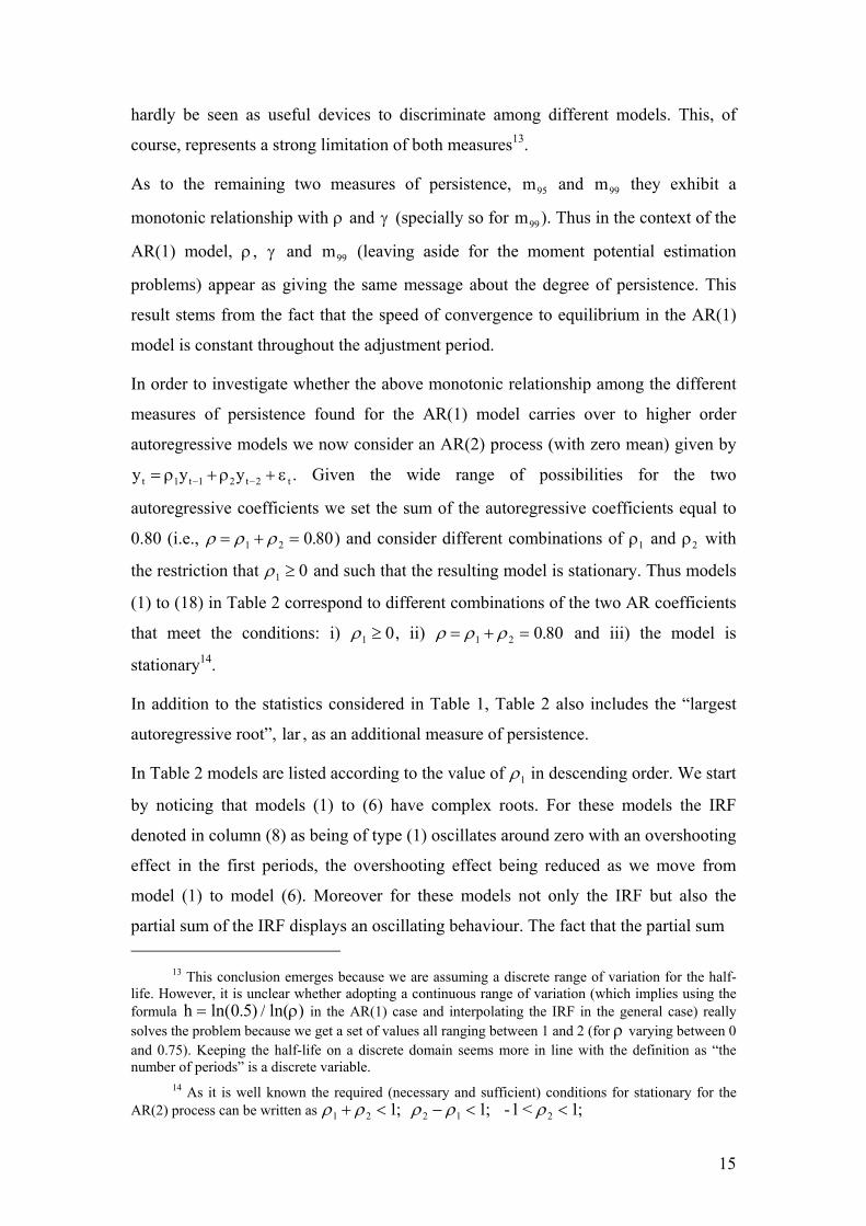
hardly be seen as useful devices to discriminate among different models. This, of

course, represents a strong limitation of both measures13.

As to the remaining two measures of persistence, m95 and m99 they exhibit a

monotonic relationship with ρ and γ (specially so for m99). Thus in the context of the

AR(1) model, ρ , γ and m99 (leaving aside for the moment potential estimation

problems) appear as giving the same message about the degree of persistence. This

result stems from the fact that the speed of convergence to equilibrium in the AR(1)

model is constant throughout the adjustment period.

In order to investigate whether the above monotonic relationship among the different

measures of persistence found for the AR(1) model carries over to higher order

autoregressive models we now consider an AR(2) process (with zero mean) given by

ty y yt t t= + +− −ρ ρ1 1 2 2 ε . Given the wide range of possibilities for the two

autoregressive coefficients we set the sum of the autoregressive coefficients equal to

0.80 (i.e., ρ ρ ρ= + =1 2 0 80. ) and consider different combinations of ρ and ρ with

the restriction that 1 2

ρ1 ≥ 0 and such that the resulting model is stationary. Thus models

(1) to (18) in Table 2 correspond to different combinations of the two AR coefficients

that meet the conditions: i) ρ1 0≥ , ii) ρ ρ ρ= + =1 2 0 80. and iii) the model is

stationary14.

In addition to the statistics considered in Table 1, Table 2 also includes the “largest

autoregressive root”, lar , as an additional measure of persistence.

In Table 2 models are listed according to the value of ρ1 in descending order. We start

by noticing that models (1) to (6) have complex roots. For these models the IRF

denoted in column (8) as being of type (1) oscillates around zero with an overshooting

effect in the first periods, the overshooting effect being reduced as we move from

model (1) to model (6). Moreover for these models not only the IRF but also the

partial sum of the IRF displays an oscillating behaviour. The fact that the partial sum

13 This conclusion emerges because we are assuming a discrete range of variation for the half-life. However, it is unclear whether adopting a continuous range of variation (which implies using the formula h = ln( . ) / ln( )0 5 ρ in the AR(1) case and interpolating the IRF in the general case) really solves the problem because we get a set of values all ranging between 1 and 2 (for ρ varying between 0 and 0.75). Keeping the half-life on a discrete domain seems more in line with the definition as “the number of periods” is a discrete variable.

14 As it is well known the required (necessary and sufficient) conditions for stationary for the AR(2) process can be written as ρ ρ ρ ρ ρ1 2 2 1 21 1+ 1< − < <; ; -1 < ;

15

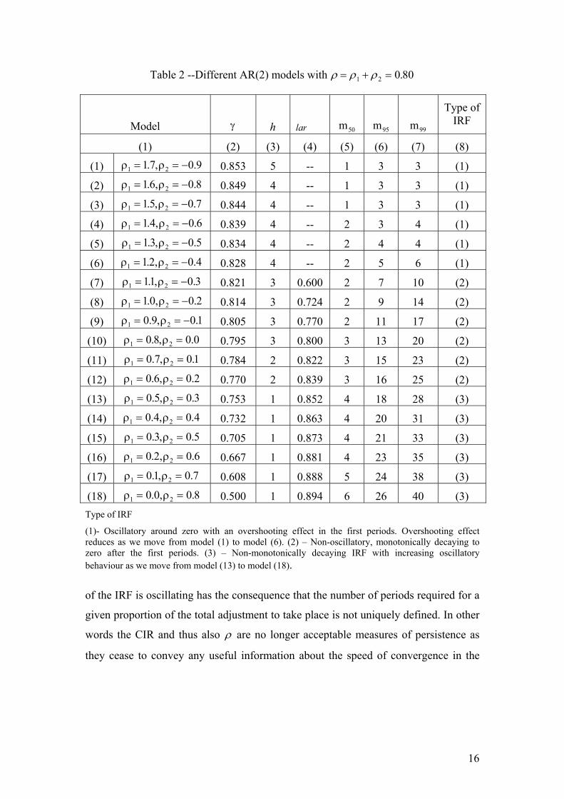
Table 2 --Different AR(2) models with ρ ρ ρ= + =1 2 0 80.

Model

γ

h

lar

m50

m95

m99

Type of IRF

(1) (2) (3) (4) (5) (6) (7) (8)

(1) ρ ρ1 21 7 0 9= = −. , . 0.853 5 -- 1 3 3 (1)

(2) ρ ρ1 21 6 0 8= = −. , . 0.849 4 -- 1 3 3 (1)

(3) ρ ρ1 21 5 0 7= = −. , . 0.844 4 -- 1 3 3 (1)

(4) ρ ρ1 21= 0 6= −.4, . 0.839 4 -- 2 3 4 (1)

(5) ρ ρ1 21 3 0 5= = −. , . 0.834 4 -- 2 4 4 (1)

(6) ρ ρ1 21 2 0= = −. , .4 0.828 4 -- 2 5 6 (1)

(7) ρ ρ1 211 0 3= = −. , . 0.821 3 0.600 2 7 10 (2)

(8) ρ ρ1 21 0 0 2= = −. , . 0.814 3 0.724 2 9 14 (2)

(9) ρ ρ1 20 9 0 1= = −. , . 0.805 3 0.770 2 11 17 (2)

(10) ρ ρ1 20 8 0 0= =. , . 0.795 3 0.800 3 13 20 (2)

(11) ρ ρ1 20 7 0 1= =. , . 0.784 2 0.822 3 15 23 (2)

(12) ρ ρ1 20 6 0 2= =. , . 0.770 2 0.839 3 16 25 (2)

(13) ρ ρ1 20 5 0 3= =. , . 0.753 1 0.852 4 18 28 (3)

(14) ρ ρ1 20= =.4, .40 0.732 1 0.863 4 20 31 (3)

(15) ρ ρ1 20 3 0 5= =. , . 0.705 1 0.873 4 21 33 (3)

(16) ρ ρ1 20 2 0 6= =. , . 0.667 1 0.881 4 23 35 (3)

(17) ρ ρ1 20 1 0 7= =. , . 0.608 1 0.888 5 24 38 (3)

(18) ρ ρ1 20 0 0 8= =. , . 0.500 1 0.894 6 26 40 (3) Type of IRF

(1)- Oscillatory around zero with an overshooting effect in the first periods. Overshooting effect reduces as we move from model (1) to model (6). (2) – Non-oscillatory, monotonically decaying to zero after the first periods. (3) – Non-monotonically decaying IRF with increasing oscillatory behaviour as we move from model (13) to model (18).

of the IRF is oscillating has the consequence that the number of periods required for a

given proportion of the total adjustment to take place is not uniquely defined. In other

words the CIR and thus also ρ are no longer acceptable measures of persistence as

they cease to convey any useful information about the speed of convergence in the

16

impulse response function. Of course, this criticism also applies to the half-life, m50,

m95 and m9915.

For models (7) to (12) the IRF denoted as type (2) in column (8) is non-oscillatory

and monotonically decaying to zero after the first periods. However, in the first

periods the IRF with the exception of model (10) (which corresponds to the special

case of the AR(1) process) exhibits a non-constant speed of convergence. Finally for

models (13) to (18) the IRF denoted as type (3) in column (8) is a non-monotonic

decaying process with increasing oscillatory behaviour as we move from model (13)

to model (18). Despite the non-monotonic behaviour of the IRF function during the

first periods the corresponding CIR increases monotonically for models (7) to (18).

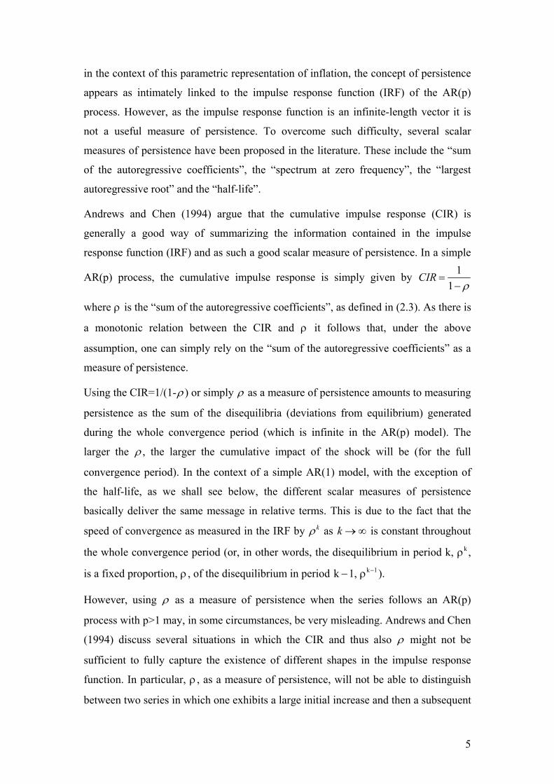
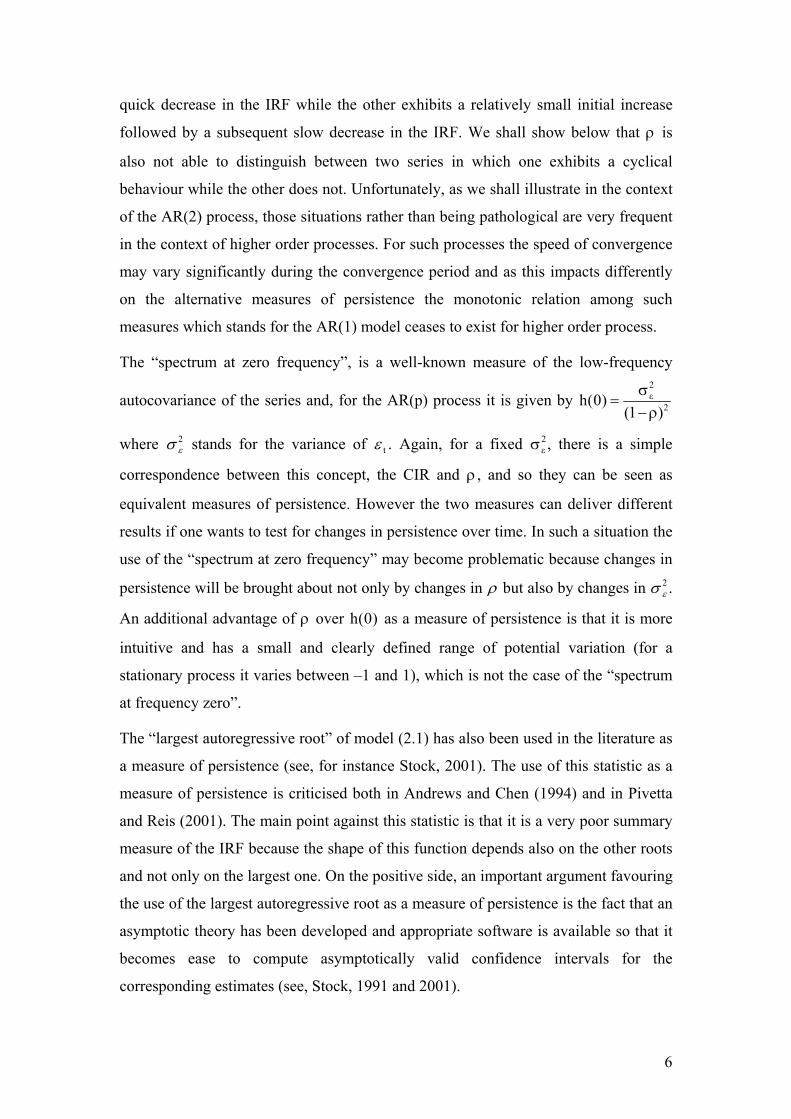
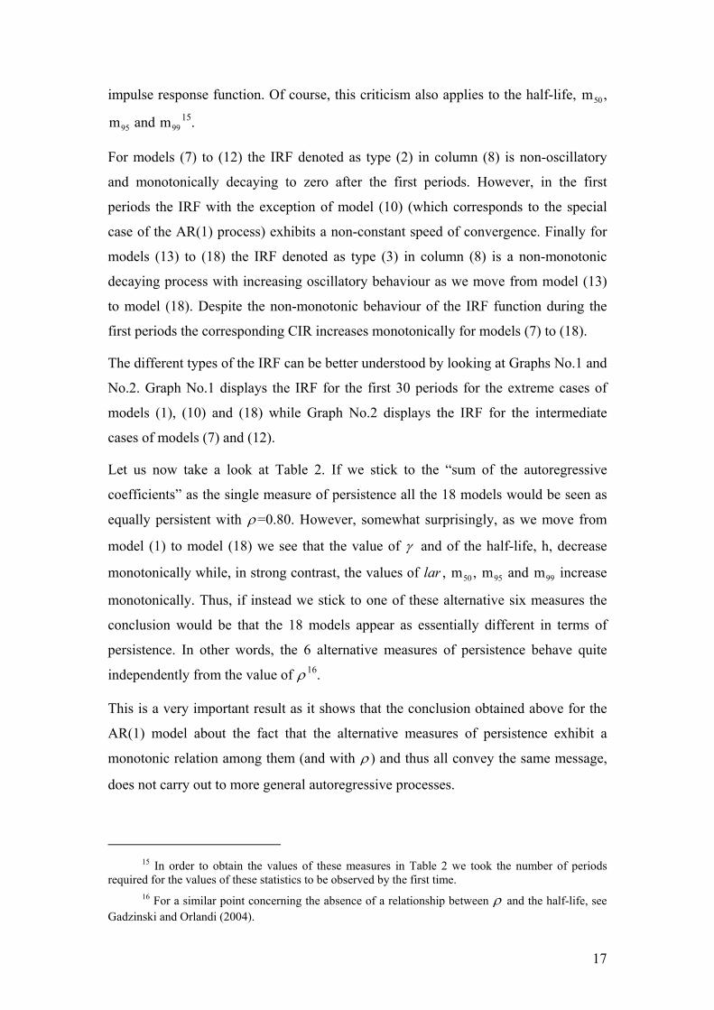
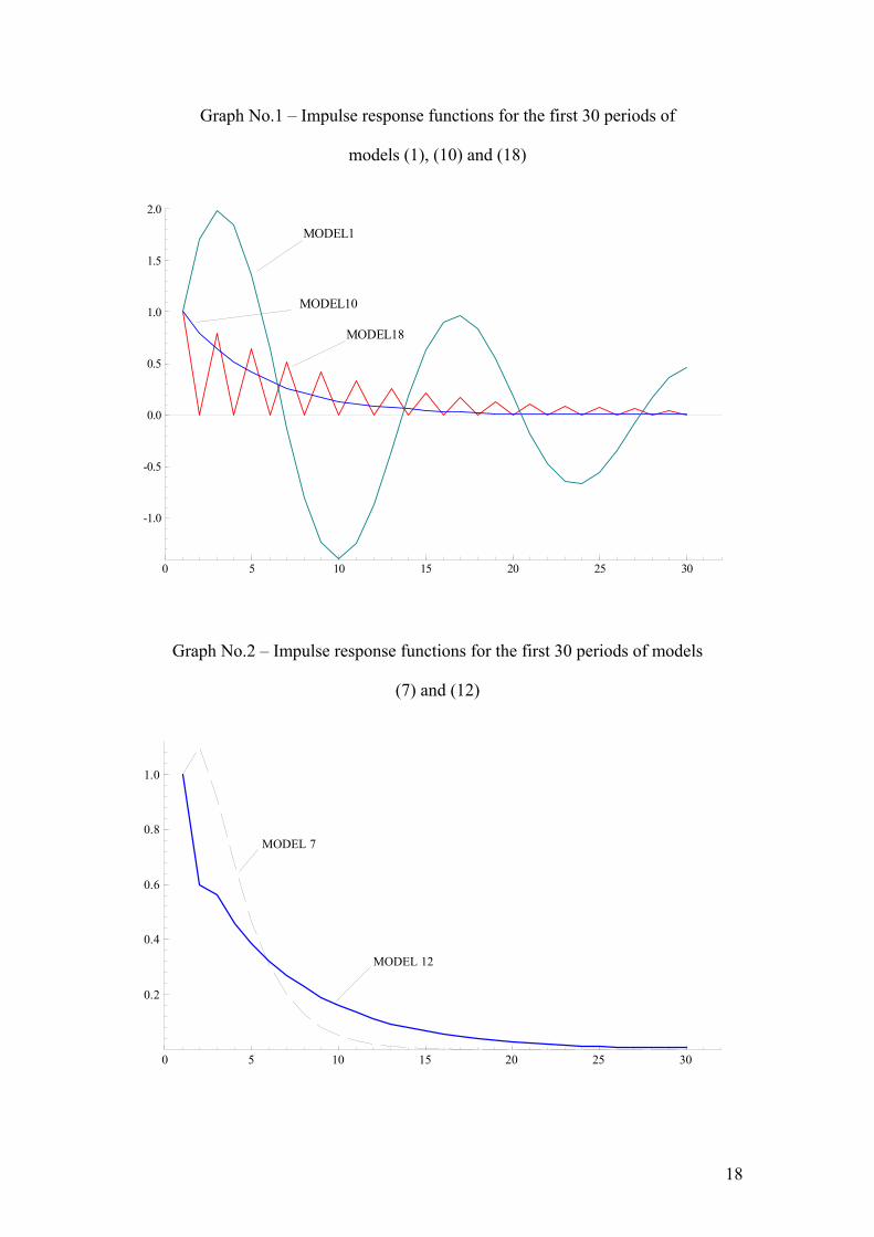
The different types of the IRF can be better understood by looking at Graphs No.1 and

No.2. Graph No.1 displays the IRF for the first 30 periods for the extreme cases of

models (1), (10) and (18) while Graph No.2 displays the IRF for the intermediate

cases of models (7) and (12).

Let us now take a look at Table 2. If we stick to the “sum of the autoregressive

coefficients” as the single measure of persistence all the 18 models would be seen as

equally persistent with ρ=0.80. However, somewhat surprisingly, as we move from

model (1) to model (18) we see that the value of γ and of the half-life, h, decrease

monotonically while, in strong contrast, the values of lar , m50, m95 and m99 increase

monotonically. Thus, if instead we stick to one of these alternative six measures the

conclusion would be that the 18 models appear as essentially different in terms of

persistence. In other words, the 6 alternative measures of persistence behave quite

independently from the value of ρ 16.

This is a very important result as it shows that the conclusion obtained above for the

AR(1) model about the fact that the alternative measures of persistence exhibit a

monotonic relation among them (and with ρ ) and thus all convey the same message,

does not carry out to more general autoregressive processes.

15 In order to obtain the values of these measures in Table 2 we took the number of periods

required for the values of these statistics to be observed by the first time. 16 For a similar point concerning the absence of a relationship between ρ and the half-life, see

Gadzinski and Orlandi (2004).

17

Graph No.1 – Impulse response functions for the first 30 periods of

models (1), (10) and (18)

0 5 10 15 20 25 30

-1.0

-0.5

0.0

0.5

1.0

1.5

2.0

MODEL1

MODEL10

MODEL18

Graph No.2 – Impulse response functions for the first 30 periods of models

(7) and (12)

0 5 10 15 20 25 30

0.2

0.4

0.6

0.8

1.0

MODEL 7

MODEL 12

18

The idea that the scalar measures of persistence could in some specific situations be

very misleading about the true level of persistence is, of course, not new (see

Andrews and Chen, 1994, and the discussion in section 2 above). What seems to be

new (at least for the authors) is the extension of the problem. More than saying that in

some special cases the CIR (and thus all the measures based on the CIR as ρ , m50,

m95 or m99) is not a good summary measure of the information contained in the IRF

(and thus is not a good measure of persistence) it seems more appropriate to state that

with the exception of the very special case of the AR(1) model, the scalar measures of

persistence for the general autoregressive model may be very misleading either by

suggesting the presence of a strong degree of persistence when it is absent or by

suggesting the absence of significant persistence when it is present.

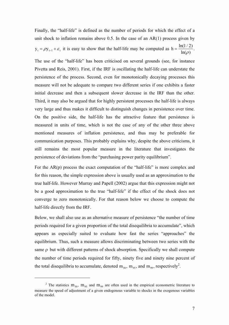
For instance, if we take a look at Graph No.3, which displays a realization of models

(1), (10) and (18) with 80 observations it seems difficult to argue that the three

models, despite having the same ρ=0.8, should be seen as equally persistent, given

the disparate values for the 6 measures of persistence in Table 217. If we think of

persistence as the frequency of mean reversion we see that mean reversion in model

(10) and model (18) is clearly higher than in model (1) suggesting thus that

persistence is lower in those two models. On the other hand, we also see that mean

reversion in model (18) is higher than in model (10)18. The different degree of mean

reversion among the 18 models in Table 2 can be inferred from column (2), which

reports the values of γ for each model. We can see that γ starting with model (1)

decreases monotonically from a value as high as 0.853 (signalling a very persistent

process) to a figure as low as 0.50 which signals a model with zero persistence.

We expect γ to be equal to 0.5 when a white noise process generates the data, but by

simply eyeballing the series we see that model (18) in Graph No.3 does not behave

like a white noise. Rather it seems to display a kind of cyclical behaviour, which

makes the process to cross the mean at irregular intervals, but such that on average it

crosses the mean as often as if it were a white noise. This means that γ does not

distinguish between a process with a low ρ (close to a white noise behaviour) and a

17 The three series in graph No.3 were generated using the same series of residuals, which in turn were generated from the N(0,1) distribution.

18 Notice that the two models behave similarly during most of the sample but mean reversion in model (18) is higher for observations 30-34 and 60-64 suggesting that persistence in model (18) is lower.

19

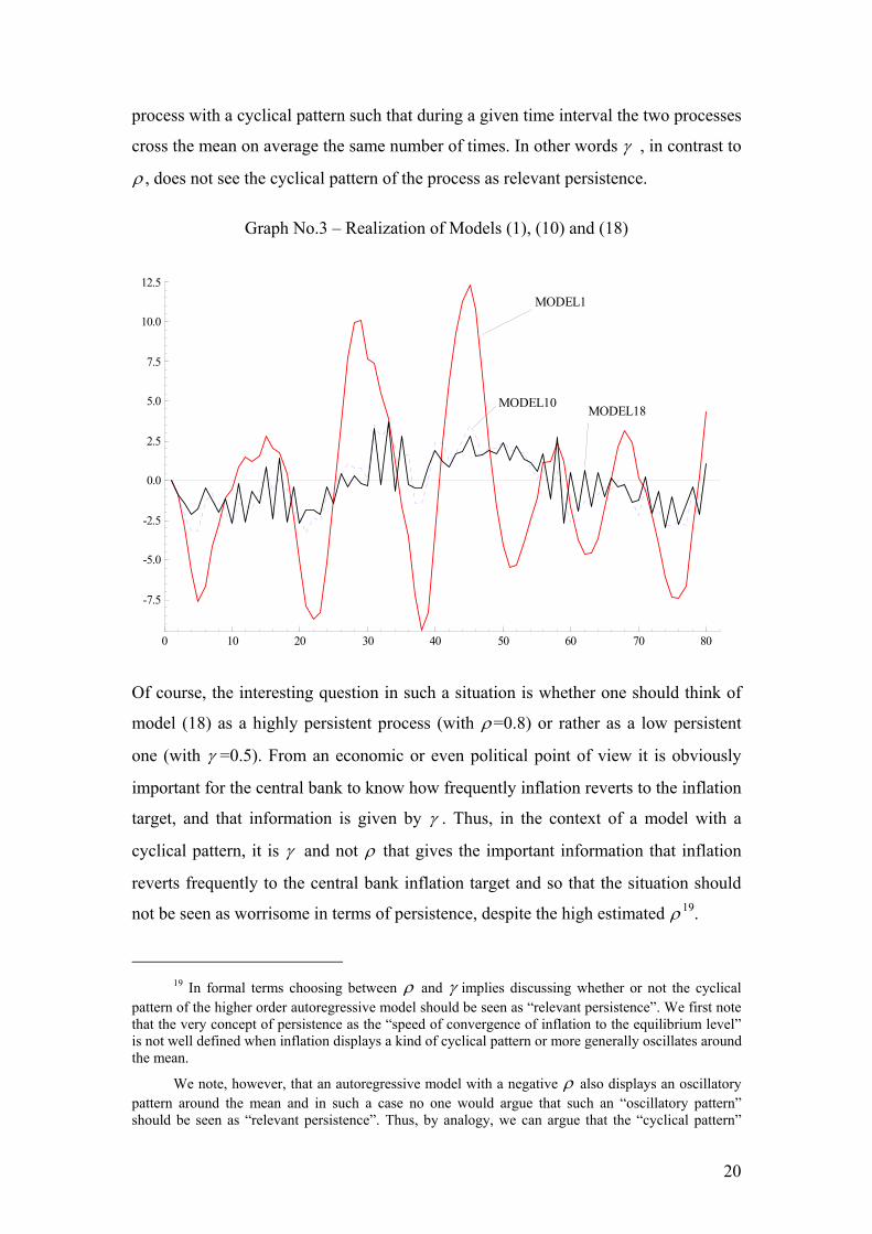
process with a cyclical pattern such that during a given time interval the two processes

cross the mean on average the same number of times. In other words γ , in contrast to

ρ , does not see the cyclical pattern of the process as relevant persistence.

-7

-5

-2

10

12

EL1

Graph No.3 – Realization of Models (1), (10) and (18)

0 10 20 30 40 50 60 70 80

.5

.0

.5

0.0

2.5

5.0

7.5

.0

.5MODEL1

MODEL10 MOD 8

Of course, the interesting question in such a situation is whether one should think of

model (18) as a highly persistent process (with ρ=0.8) or rather as a low persistent

one (with γ =0.5). From an economic or even political point of view it is obviously

important for the central bank to know how frequently inflation reverts to the inflation

target, and that information is given by γ . Thus, in the context of a model with a

cyclical pattern, it is γ and not ρ that gives the important information that inflation

reverts frequently to the central bank inflation target and so that the situation should

not be seen as worrisome in terms of persistence, despite the high estimated ρ 19.

19 In formal terms choosing between ρ and γ implies discussing whether or not the cyclical

pattern of the higher order autoregressive model should be seen as “relevant persistence”. We first note that the very concept of persistence as the “speed of convergence of inflation to the equilibrium level” is not well defined when inflation displays a kind of cyclical pattern or more generally oscillates around the mean.

We note, however, that an autoregressive model with a negative ρ also displays an oscillatory pattern around the mean and in such a case no one would argue that such an “oscillatory pattern” should be seen as “relevant persistence”. Thus, by analogy, we can argue that the “cyclical pattern”

20

By looking at the IFRs of the 18 AR(2) processes we see that it is the non-constant

speed of convergence in the IRF which gives rise to the diverging results for the

different measures of persistence. In particular, we note that the values of γ for

models (8), (9), (11) and (12) which are the ones with an IRF closer to that of the

AR(1) process (model (10)) are very close to the value obtained for the AR(1) case.

Thus, we can infer that in general what matters for the interpretation of the results is

whether or not the IRF closely reproduces the constant speed characteristic of the IRF

of the AR(1) model independently of the order of the underlying process. In other

words, we can expect the relationship between ρ and γ in Table 1 to hold for higher

processes provided the IRF displays a (close to a) constant speed of convergence

throughout the adjustment period. In this sense comparing ρ and γ may shed some

light on the characteristics of the IRF.

In finalizing this section we stress the idea that relying exclusively on ρ , as the single

measure of persistence, as it is current practice in the empirical literature, does not

allow uncovering important features of inflation persistence in the context of higher

order autoregressive processes. In order to better characterise inflation persistence in

such a context it seems advisable to compute at least two alternative scalar measures

of persistence capable of delivering complementary information. In this regard using

γ and ρ as companion measures of persistence allows obtaining useful information to

characterise the degree of persistence that cannot be extracted from γ or ρ in

isolation. We have seen that a value of ρ clearly above to what could be expected

given the value of γ could be signalling a cyclical pattern in the DGP. We shall see

below that an estimate of ρ clearly below the value of $γ may be seen as a signal of

significant biases in ρ stemming from the presence of additive outliers in the data or

from model misspecifications.

$

5. SOME MONTE CARLO EVIDENCE ON THE FINITE SAMPLE

PROPERTIES OF $γ AND $ρ .

In this section we use some Monte Carlo experiments in order to investigate the

properties of $γ and ρ regarding i) unbiasedness and consistency, ii) finite sample $

should also not be seen as “relevant persistence” and thus, γ should be preferred to ρ , as a measure of persistence.

21

performance of their asymptotic distribution, iii) robustness to outliers and iv)

robustness against model misspecifications. These properties are investigated in the

context of the AR(1) and AR(2) processes considered in section 4.

From the discussion in section 3 we may expect the information about the mean of the

process to be statistically relevant for persistence evaluation. For this reason, below

we distinguish the situation in which the mean is known from the situation in which

the mean is unknown. Assuming that the mean is known may be realistic for those

countries for which an inflation targeting monetary policy was implemented and an

explicit inflation target was announced. In this case, the true mean of the series can be

computed exogenously to realised inflation and is given by the publicly announced

inflation target. However, for most countries the exact (implicit) inflation target used

by the central bank when setting monetary policy is unknown. In theses cases the

mean must be computed from realised inflation and this implies endogenising the

central bank inflation target. As we shall see below this may have noticeable

consequences for the process of persistence evaluation if the sample is not very large.

5.1 – Unbiasedness and consistency

Let us start by assuming that true mean of the process is known. Under such

circumstances we can extract the mean from realised inflation and assume that the

true model does not have an intercept or that the mean of the process is zero20.

To proceed we start by defining an experiment that constructs the data to follow an

AR(1) process (with no intercept) given by ty yt t= +−ρ ε1 for ρ ranging between 0

and 1 and where the errors are serially uncorrelated standard normal variables. The

data are generated by setting y =0 and creating T+100 observations, discarding the

first 100 observations to remove the effect of the initial conditions. Samples of size

T=50, 75, 100, 150, 250, 500 and 1000 are used in the experiments. Each experiment

−100

20 Note that under this assumption it does not matter whether we think of the mean as a constant

or time varying. Thus conclusions derived below, under the assumption that the mean is known, are valid no matter how the mean is defined (constant, piecewise constant or time varying). However, the conclusions for the case of unknown mean assume that the (unknown) mean is constant throughout the sample period.

22

is replicated 10,000 times in order to create the sampling distributions of the

estimators21.

It is known that the sampling distribution of the least squares estimator of ρ , $ρ ,

(namely the expectation and standard deviation of $ρ) depends on the initial value of

the process (y ) (see, for instance, Evans and Savin (1981)). For stationary processes

Sawa (1978) argues that there is no noticeable difference whether one assumes that

the initial value is a fixed constant or y is a drawing from a stationary distribution. In

our case we implicitly assume that the process has started somewhere in the past

( =0) so that for estimation purposes our initial value (y ) may be seen as a

random normal variable with Var

0

0

y−100 0

y( ) / (02 1 )2= −σ ρε

−10

22. Some simulations were carried

out in which different values for y were assumed. As expected such changes had

no noticeable impact on the estimated statistics.

0

The output of the experiment for T=100 is displayed in Table 3. For values of ρ

ranging between 0 and 1, column (2) reports the average value for the Monte Carlo

OLS estimates of the ρ parameter (ρ ) and column (3) the median of these estimates

(ρ$ m ). Similarly, column (6) reports the values of γ (taken from Table 1), column (7)

the average value of the Monte Carlo estimates of γ (γ ), column (8) the

corresponding median ( $γ m ) and column (9) the standard error of $γ 23.

From Table 3 we can see that the OLS estimator of ρ is slightly (mean) downward

biased and that the absolute bias increases as ρ increases, as expected. From column

(3) we also see that the median of the least squares estimates ( $ρm ) is higher than the

mean of the estimates (ρ ) but still lower than ρ . Such evidence is consistent with the

result in the literature that the finite sample distribution of $ρ besides being downward

biased is also negatively skewed (see, Sawa, 1978, Phillips, 1977, Evans and Savin,

1981, Andrews, 1993, Andrews and Chen, 1994).

21 All the experiments in this paper are replicated 10,000 times with the data generated by

setting =0 and creating T+100 observations, discarding the first 100 observations to remove the effect of the initial conditions The replications were carried out in TSP 4.5.

y−100

22 In rigour under the assumption that =0 and that y−100 ε t

/ is i.i.d. N(0, σ ) we have

which reduces to var(ε2

var( ) ( )( )y x0

2 2 100 21 1= − − −σ ρ ρε1 ) ( )y0

2 21= −σ ρε as ρ . 2 0≈100x

23 We note that the standard error of $γ and $ρ is the standard error of the series composed of the 10,000 estimates of γ and ρ , respectively.

23

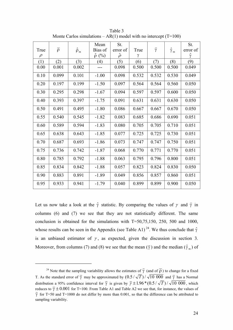
Table 3 Monte Carlos simulations – AR(1) model with no intercept (T=100)

True ρ

ρ

$ρm

Mean Bias of

(%) $ρ

St. error of

$ρ

True γ

γ

$γ m

St. error of

$γ (1) (2) (3) (4) (5) (6) (7) (8) (9)

0.00 0.001 0.002 --- 0.098 0.500 0.500 0.500 0.049

0.10 0.099 0.101 -1.00 0.098 0.532 0.532 0.530 0.049

0.20 0.197 0.199 -1.50 0.097 0.564 0.564 0.560 0.050

0.30 0.295 0.298 -1.67 0.094 0.597 0.597 0.600 0.050

0.40 0.393 0.397 -1.75 0.091 0.631 0.631 0.630 0.050

0.50 0.491 0.495 -1.80 0.086 0.667 0.667 0.670 0.050

0.55 0.540 0.545 -1.82 0.083 0.685 0.686 0.690 0.051

0.60 0.589 0.594 -1.83 0.080 0.705 0.705 0.710 0.051

0.65 0.638 0.643 -1.85 0.077 0.725 0.725 0.730 0.051

0.70 0.687 0.693 -1.86 0.073 0.747 0.747 0.750 0.051

0.75 0.736 0.742 -1.87 0.068 0.770 0.771 0.770 0.051

0.80 0.785 0.792 -1.88 0.063 0.795 0.796 0.800 0.051

0.85 0.834 0.842 -1.88 0.057 0.823 0.824 0.830 0.050

0.90 0.883 0.891 -1.89 0.049 0.856 0.857 0.860 0.051

0.95 0.933 0.941 -1.79 0.040 0.899 0.899 0.900 0.050

Let us now take a look at the $γ statistic. By comparing the values of γ and γ in

columns (6) and (7) we see that they are not statistically different. The same

conclusion is obtained for the simulations with T=50,75,150, 250, 500 and 1000,

whose results can be seen in the Appendix (see Table A1) 24. We thus conclude that $γ

is an unbiased estimator of γ , as expected, given the discussion in section 3.

Moreover, from columns (7) and (8) we see that the mean (γ ) and the median ( $γ m ) of

24 Note that the sampling variability allows the estimates of γ (and of ρ ) to change for a fixed

T. As the standard error of γ may be approximated by ( . and / ) /0 5 10 000T γ has a Normal distribution a 95% confidence interval for γ is given by γ ±1 96 0 5 10 000. *( . / ) /T , which reduces to γ ± 0 001. for T=100. From Table A1 and Table A2 we see that, for instance, the values of γ for T=50 and T=1000 do not differ by more than 0.001, so that the difference can be attributed to sampling variability.

24

$γ seem to coincide, which suggests that the distribution of $γ is essentially

symmetric25.

Table 4 Monte Carlo simulations – AR(1) model with an intercept (T=100)

True ρ

ρ

$ρm

Mean Bias of

(%) $ρ

True γ

γ

$γ m

Mean Bias of $γ (%)

St. error of

$γ

(1) (2) (3) (4) (5) (6) (7) (8) (9) 0.00 -0.010 -0.008 --- 0.500 0.497 0.500 -0.60 0.049

0.10 0.087 0.089 -12.54 0.532 0.528 0.530 -0.75 0.049

0.20 0.184 0.187 -7.78 0.564 0.560 0.560 -0.71 0.049

0.30 0.281 0.285 -6.19 0.597 0.592 0.590 -0.84 0.050

0.40 0.378 0.383 -5.41 0.631 0.626 0.630 -0.80 0.050

0.50 0.475 0.480 -4.95 0.667 0.661 0.660 -0.90 0.051

0.55 0.524 0.528 -4.79 0.685 0.679 0.680 -0.88 0.051

0.60 0.572 0.577 -4.66 0.705 0.698 0.700 -1.00 0.051

0.65 0.620 0.626 -4.55 0.725 0.718 0.720 -0.97 0.051

0.70 0.669 0.675 -4.47 0.747 0.739 0.740 -1.07 0.051

0.75 0.717 0.724 -4.40 0.770 0.762 0.760 -1.04 0.051

0.80 0.765 0.772 -4.36 0.795 0.786 0.790 -1.13 0.051

0.85 0.813 0.821 -4.34 0.823 0.812 0.810 -1.34 0.051

0.90 0.861 0.869 -4.37 0.856 0.842 0.850 -1.64 0.052

0.95 0.907 0.916 -4.52 0.899 0.878 0.880 -2.34 0.052

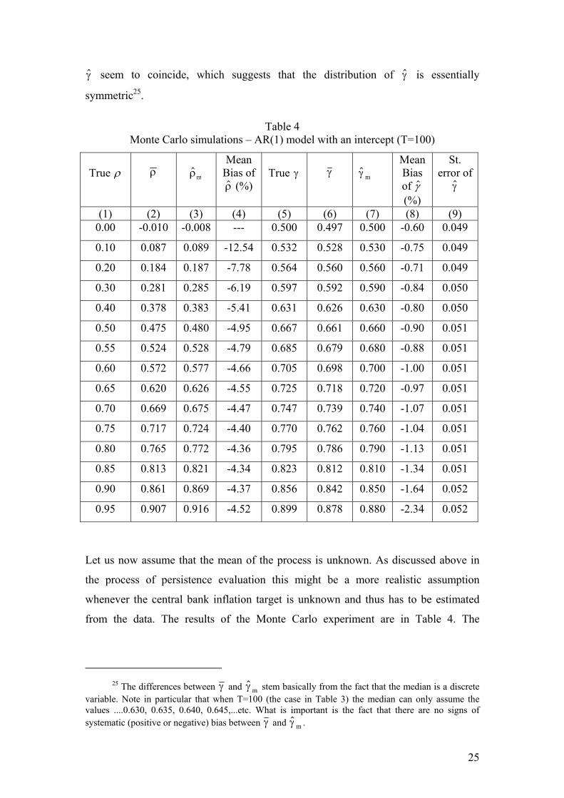
Let us now assume that the mean of the process is unknown. As discussed above in

the process of persistence evaluation this might be a more realistic assumption

whenever the central bank inflation target is unknown and thus has to be estimated

from the data. The results of the Monte Carlo experiment are in Table 4. The

25 The differences between γ and $γ m stem basically from the fact that the median is a discrete

variable. Note in particular that when T=100 (the case in Table 3) the median can only assume the values ....0.630, 0.635, 0.640, 0.645,...etc. What is important is the fact that there are no signs of systematic (positive or negative) bias between γ and $γ m .

25

estimates ρ were obtained by estimating the AR(1) model with an intercept and those

of

$

$γ were computed conditional on the estimated mean26.

Looking at Table 4 we see that the downward bias of OLS estimator has now

significant damaging consequences on the expected estimates of ρ . In fact, the bias

has now more than doubled vis-à-vis the situation in Table 3, confirming the claim in

Sawa (1978) and Andrews (1993) that the bias of $ρ is more acute when one assumes

that the mean of the process is unknown and has to be estimated from the data using a

model with an intercept. In empirical applications this downward bias of $ρ will

naturally translate into all measures of persistence that are computed using an estimate

of ρ (the half-life, m50, m95 and m99 in Table 1). This is the case for which it might

be worth using the “approximated median unbiased estimator” suggested in Andrews

(1994).27

As to the $γ statistic we see that it also appears slightly downward biased as expected

given the discussion in section 3. This result is intuitive, as the estimator of the mean

(the estimated average) can only increase mean reversion vis-à-vis the situation with

the true mean, and thus reduce the estimated γ .

Let us now briefly take a look at the AR(2) process. In our Monte Carlo experiment

we consider as our DGP the same 18 models of section 4 for which ρ ρ ρ= + =1 2 0 80.

with a zero intercept and serially uncorrelated standard normal errors. The output of

the experiment is in Table 5. Column (2) reports the average of the OLS estimates of

(ρ ρ ) and column (7) the average value for the $γ statistic (γ ) obtained under the

assumption that the mean of the process is known, i.e., by estimating an AR(2)

process without an intercept and computing $γ assuming a zero mean for the process.

Column (4) and column (8) report the corresponding values of these statistics under

the assumption that the mean is unknown, i.e., by estimating an AR(2) model with an

intercept and computing $γ conditional on the estimated mean. To facilitate

comparisons, column (6) reports the values of γ taken from Table 2.

26 Numbers in the table were obtained by generating the model y z with

t

t t= +0 01.z zt t= +−ρ ε1 . We note that the sampling distributions of $ρ and $γ do not depend on the value of mean, but simply on the fact that mean is unknown and has to be estimated.

27 However, we shall argue below that far most important biases are brought into the least squares estimator due to potential model misspecifications or to the presence of additive outliers but that such biases may not be overcome by resorting the median unbiased estimator.

26

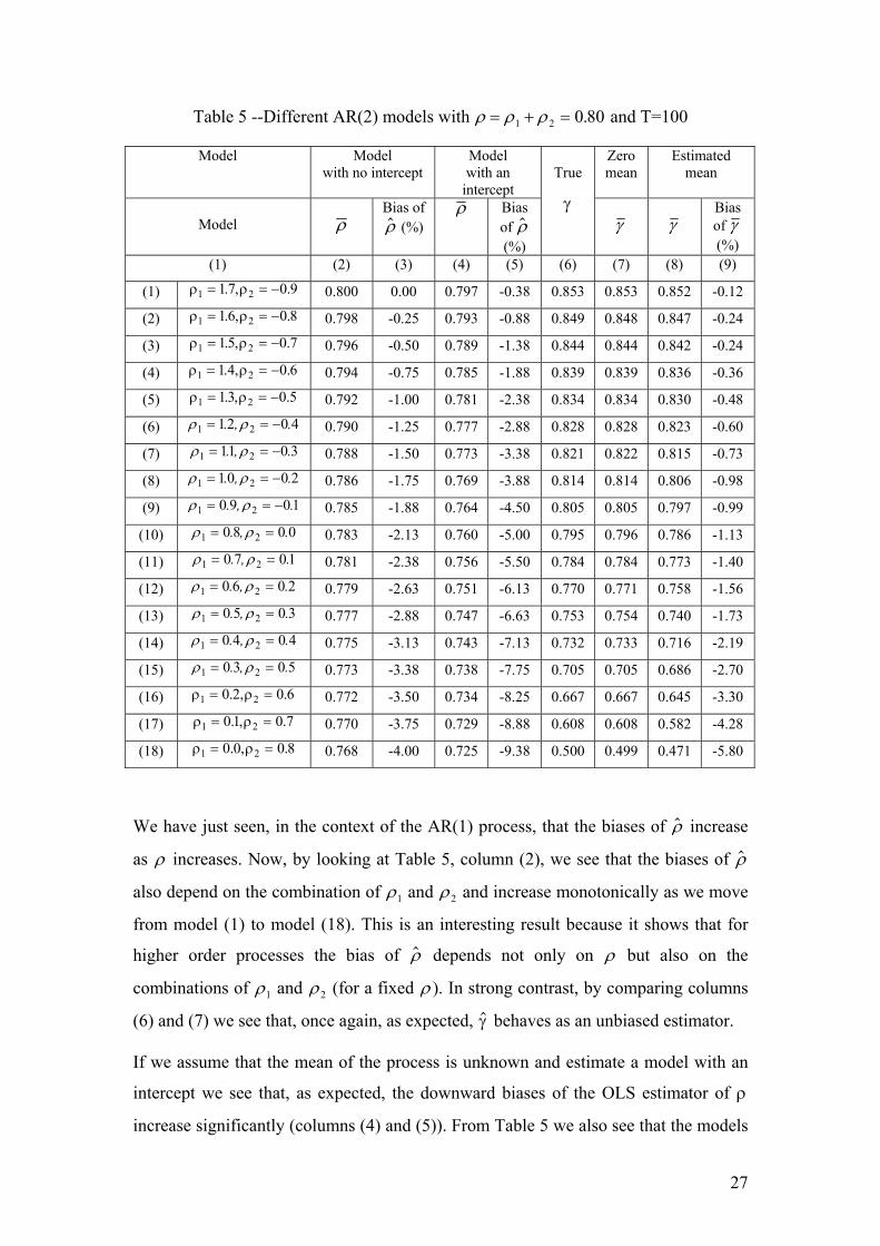
Table 5 --Different AR(2) models with ρ ρ ρ= + =1 2 0 80. and T=100

Model Model with no intercept

Model with an

intercept

Zero mean

Estimated mean

Model

ρ

Bias of $ρ (%)

ρ Bias of $ρ (%)

True

γ

γ γ

Bias of γ (%)

(1) (2) (3) (4) (5) (6) (7) (8) (9)

(1) ρ ρ1 21 7 0 9= = −. , . 0.800 0.00 0.797 -0.38 0.853 0.853 0.852 -0.12

(2) ρ ρ1 21 6 0 8= = −. , . 0.798 -0.25 0.793 -0.88 0.849 0.848 0.847 -0.24

(3) ρ ρ1 21 5 0 7= = −. , . 0.796 -0.50 0.789 -1.38 0.844 0.844 0.842 -0.24

(4) ρ ρ1 21= 0 6= −.4, . 0.794 -0.75 0.785 -1.88 0.839 0.839 0.836 -0.36

(5) ρ ρ1 213 0 5= = −. , . 0.792 -1.00 0.781 -2.38 0.834 0.834 0.830 -0.48

(6) ρ ρ1 212 0 4= = −. , . 0.790 -1.25 0.777 -2.88 0.828 0.828 0.823 -0.60

(7) ρ ρ1 211 0 3= = −. , . 0.788 -1.50 0.773 -3.38 0.821 0.822 0.815 -0.73

(8) ρ ρ1 21 0 0 2= = −. , . 0.786 -1.75 0.769 -3.88 0.814 0.814 0.806 -0.98

(9) ρ ρ1 20 9 01= = −. , . 0.785 -1.88 0.764 -4.50 0.805 0.805 0.797 -0.99

(10) ρ ρ1 20 8 0 0= =. , . 0.783 -2.13 0.760 -5.00 0.795 0.796 0.786 -1.13

(11) ρ ρ1 20 7 01= =. , . 0.781 -2.38 0.756 -5.50 0.784 0.784 0.773 -1.40

(12) ρ ρ1 20 6 0 2= =. , . 0.779 -2.63 0.751 -6.13 0.770 0.771 0.758 -1.56

(13) ρ ρ1 20 5 0 3= =. , . 0.777 -2.88 0.747 -6.63 0.753 0.754 0.740 -1.73

(14) ρ ρ1 20 4 0 4= =. , . 0.775 -3.13 0.743 -7.13 0.732 0.733 0.716 -2.19

(15) ρ ρ1 20 3 0 5= =. , . 0.773 -3.38 0.738 -7.75 0.705 0.705 0.686 -2.70

(16) ρ ρ1 20 2 0 6= =. , . 0.772 -3.50 0.734 -8.25 0.667 0.667 0.645 -3.30

(17) ρ ρ1 20 1 0 7= =. , . 0.770 -3.75 0.729 -8.88 0.608 0.608 0.582 -4.28

(18) ρ ρ1 20 0 0 8= =. , . 0.768 -4.00 0.725 -9.38 0.500 0.499 0.471 -5.80

We have just seen, in the context of the AR(1) process, that the biases of $ρ increase

as ρ increases. Now, by looking at Table 5, column (2), we see that the biases of $ρ

also depend on the combination of ρ1 and ρ2 and increase monotonically as we move

from model (1) to model (18). This is an interesting result because it shows that for

higher order processes the bias of $ρ depends not only on ρ but also on the

combinations of ρ1 and ρ2 (for a fixed ρ ). In strong contrast, by comparing columns

(6) and (7) we see that, once again, as expected, $γ behaves as an unbiased estimator.

If we assume that the mean of the process is unknown and estimate a model with an

intercept we see that, as expected, the downward biases of the OLS estimator of ρ

increase significantly (columns (4) and (5)). From Table 5 we also see that the models

27

which we expect to be more realistic in empirical terms (the ones for which ρ1<1) are

also the ones for which the biases are larger. As regards the $γ statistic we see that,

similarly to the AR(1) case, a small downward bias emerges (column (9)) and that the

bias increases as we move from model (1) to model (18). However it is always

smaller than the bias displayed by $ρ (column (5)).

$γ

$γ

$γ b

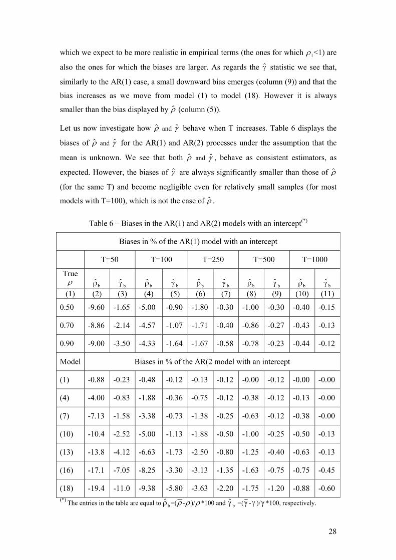
Let us now investigate how $ρ and behave when T increases. Table 6 displays the

biases of $ρ and $γ for the AR(1) and AR(2) processes under the assumption that the

mean is unknown. We see that both $ρ and $γ , behave as consistent estimators, as

expected. However, the biases of are always significantly smaller than those of $ρ

(for the same T) and become negligible even for relatively small samples (for most

models with T=100), which is not the case of $ρ .

Table 6 – Biases in the AR(1) and AR(2) models with an intercept(*)

Biases in % of the AR(1) model with an intercept

T=50 T=100 T=250 T=500 T=1000

True ρ

$ρb

$γ b

$ρb

$ρb

$γ b

$ρb

$γ b

$ρb

$γ b

(1) (2) (3) (4) (5) (6) (7) (8) (9) (10) (11)

0.50 -9.60 -1.65 -5.00 -0.90 -1.80 -0.30 -1.00 -0.30 -0.40 -0.15

0.70 -8.86 -2.14 -4.57 -1.07 -1.71 -0.40 -0.86 -0.27 -0.43 -0.13

0.90 -9.00 -3.50 -4.33 -1.64 -1.67 -0.58 -0.78 -0.23 -0.44 -0.12

Model Biases in % of the AR(2 model with an intercept

(1) -0.88 -0.23 -0.48 -0.12 -0.13 -0.12 -0.00 -0.12 -0.00 -0.00

(4) -4.00 -0.83 -1.88 -0.36 -0.75 -0.12 -0.38 -0.12 -0.13 -0.00

(7) -7.13 -1.58 -3.38 -0.73 -1.38 -0.25 -0.63 -0.12 -0.38 -0.00

(10) -10.4 -2.52 -5.00 -1.13 -1.88 -0.50 -1.00 -0.25 -0.50 -0.13

(13) -13.8 -4.12 -6.63 -1.73 -2.50 -0.80 -1.25 -0.40 -0.63 -0.13

(16) -17.1 -7.05 -8.25 -3.30 -3.13 -1.35 -1.63 -0.75 -0.75 -0.45

(18) -19.4 -11.0 -9.38 -5.80 -3.63 -2.20 -1.75 -1.20 -0.88 -0.60 (*) The entries in the table are equal to ρ =($ b ρ -ρ )/ρ*100 and $γ b =(γ -γ )/γ *100, respectively.

28

Thus, from the preceding analysis, we conclude that in the process of persistence

evaluation it may be worth distinguishing between two different possibilities. When

the central bank inflation target is known (because it is publicly announced) we may

expect to be able to estimate persistence with no (expected) bias if $γ is used or with a

small downward bias if $ρ is used. However, when the central bank inflation target is

estimated from the data, which corresponds to the common practice in the literature,

we may expect such a fact to introduce an additional downward bias into the

conventional measures of persistence. This bias might be particularly significant if

OLS estimators are used to get an estimate of ρ . The $γ statistic is very much less

affected in such a situation.

5.2 – Finite sample distributions

We know from the literature that $ρ is asymptotically normally distributed and from

section 3 that the same result is valid for $γ . However, asymptotic results are of

empirical interest only if they can provide a reasonable degree of approximation to the

finite sample distributions for the samples usually available. Thus, we now use the

output of our Monte Carlo experiments in order to evaluate the finite sample

performance of the asymptotic normality distributions for $γ and $ρ .

In order to investigate the sampling distribution of $γ and $ρ we test for skewness and

excess kurtosis in the vectors of the corresponding Monte Carlo estimates obtained for

the AR(1) and AR(2) processes as described above. For the AR(1) processes without

and with an intercept, Tables A3 and A4 in the Appendix display the p-values for the

statistics (T/6)SK2 and (T/24)KT2, where SK and KT denote the estimated skewness

and excess kurtosis, respectively28. We see that the null hypotheses of zero skewness

and zero excess kurtosis for the $γ statistic are never rejected for a 1% test. Only for

the single case of T=75 and ρ = 0 95. , in the no intercept case, is the p-value lower

than 5% for the skewness test. In stark contrast, the results for $ρ suggest that its

sampling distribution ceases to be symmetric for values of ρ larger than 0.70 and

displays an increasing degree of kurtosis for values of ρ larger than 0.80, confirming

the results in the literature that the normal approximation is quite poor in practice

28 These statistics are both distributed qui-square with 1 degree of freedom.

29

when ρ is large (Phillips, 1977, Hansen, 1999). Strangely enough there are no signs

of normality even in a sample with 1000 observations.

From Table A5 in the Appendix, which displays the p-values for the tests of zero

skewness and zero excess kurtosis for the distributions of $γ and $ρ in the AR(2) case,

we see that the null of zero skewness or zero excess kurtosis is never rejected for the $γ statistic independently of whether we assume that the mean is known or unknown.

But this is not true for the OLS estimator of ρ . As regards the distribution of $ρ , for

the process with no intercept, we see that the two null hypotheses are not rejected for

models (1) to (6) (the ones with complex roots), but are clearly rejected for models (7)

to (18) (the ones with real roots). The situation looks somewhat better for the process

with an intercept, but even in this case the null of zero skewness is rejected for models

(9) to (18).

Thus, from the above evidence we conclude that the very often-invoked asymptotic

normality of $ρ is not of much help in finite samples, but that, in strong contrast, the

asymptotic normality of $γ may be expected to work fairly well in finite samples, at

least for the type of processes investigated in this section.

5.3 – Robustness to outliers

In this section we evaluate the robustness of $γ and $ρ to the presence of outliers in the

data. Given its non-parametric characteristic we expect $γ to emerge as a more robust

statistic than $ρ . Usually two types of outliers are dealt with in the literature: the

additive outliers and the innovation outliers. The additive outliers are shocks that

affect observations in isolation due to some non-repetitive events, which may occur as

a result of measurement errors or special events (changes in VAT rates, union strikes,

for instance)29. In turn, innovation outliers are defined as extreme realisations from

the process generating the innovations, ε t , in the model.

29 Changes in VAT are, potentially, an important source of additive outliers in the series of

inflation for most EU countries. For instance, for Ireland, Italy, France and Belgium the number of revisions on VAT rates during the period 1968-2003 were 28, 19, 18 and 11, respectively (source, Directorate-General Taxation and Customs Union, EU Commission).

30

More formally, consider the AR(1) process z tzt t= +−ρ ε1 where ε t is a white noise

process and suppose that additive outliers of magnitude δ t may occur with a given

probability θ . Hence the time series we observe is

y zt t t= t+ δ λ (5.1)

where λ is a Bernoulli variable taking the value of 1 with probability θ and 0 with

probability (1-θ ). Note that the additive outlier,

t

δ t , has a one-shot effect on the

observed time series, y , and hence will produce a once-and-for-all peak in the series.

In the case of innovation outliers the time series we observe can be thought of as

being generated by

t

y yt t t t= t+ +−ρ ε δ λ1 (5.2)

so that the outlier, δ t , has an effect on the level of the series y , as any other shock t ε t ,

i.e., it will die out gradually the pace depending on ρ .

For the simple AR(1) model it has been shown (see, Lucas (1995)) that the OLS

estimator of ρ converges towards zero when the value of the additive outlier

(occurring in the middle of the sample) increases, but that under the same

circumstances the consistency of the OLS estimator of ρ is not affected in the

presence of an innovation outlier. For that reason in this section we focus on the effect

of additive outliers on $ρ and $γ .

With that purpose in mind we define the DGP as corresponding to the AR(1) model

without an intercept used in sub-section 5.1 with the addition of 5% of observations

drawn from the N(0,52) distribution. Thus, in terms of equation (5.1) we have λ =1

with probability θ=0.05 (λ =0 with probability 1-

t

t θ=0.95) and the outliers, δ , are

realisations from the N(0,5

t

2) distribution. By constructing the DGP in this way we

can, in theory, isolate the effect on $ρ coming from the usual OLS bias (reported in

Table 3) from the effect coming exclusively from the presence of outliers. Table 7

reports the results for 10.000 replications with T=100. Column (4) presents the

estimated bias for $ρ measured as a percentage deviation from the estimated values

obtained in the absence of outliers (see column (2) in Table 3). This way we are

measuring only the bias due to outliers.

31

The first important comment is that the presence of additive outliers in the data has a

devastating effect on the OLS estimators. For instance, when ρ=0.50 the expected

estimated $ρ (ρ in column (2)) is as low as 0.28 (it is equal to 0.49 when no outliers

are present) which corresponds to a downward bias of 42.15%. The effect of outliers

decreases as ρ increases, but even for values of ρ as large as 0.80 the expected $ρ is

only 0.56 (bias of –28.62%).

As regards the $γ statistic, the estimated bias (measured as a percentage deviation

from the estimated values obtained in the absence of outliers in column (7) of Table 3)

is reported in column (8). We can see that there is some downward bias as expected

(given that some outliers will imply an additional crossing of the mean), but it is quite

small. For instance, for the model with ρ=0.50 the expected $γ is now 0.654 while it

was 0.667 when no outliers were present. In general the bias of $γ due to outliers

increases as ρ increases but it always remains very small.

If instead we take a look at the average standard errors of both $ρ and $γ (columns (3)

and (7)) and compare them to the corresponding standard errors obtained in the

absence of outliers (Table 3, columns (5) and (9)), we conclude that the implications

are much stronger for the standard errors of $ρ . In fact, while the standard errors of $γ

show a small increment (the largest increase is approximately 8% and occurs for the

model with ρ=0.95), the standard errors of $ρ for higher values of ρ more than

doubled (for instance for the model with ρ=0.80, the standard error was 0.063 when

no outliers were present in the DGP and is now 0.154). The implications for the

standard deviations would naturally be reflected in, for instance, the properties of the

interquartile range of each estimator. From column (5) we see that (with the exception

of models with ρ=0.00 and ρ=0.10) the interquartile range of the OLS estimator does

not include the true ρ (nor the estimated ρ when no outliers are present). In contrast,

the interquartile range for $γ (column (9)) always includes the true γ (or the estimated

γ obtained in Table 3 when no outliers were present in the data).

Results in Table 7 are, of course, specific to the particular way we generated the data,

and less extreme outliers are expected to have less damaging consequences for $ρ .

However, the exercise carried out shows that in general we can expect $γ to be more

robust to the presence of additive outliers in the data than the OLS estimator of ρ .

32

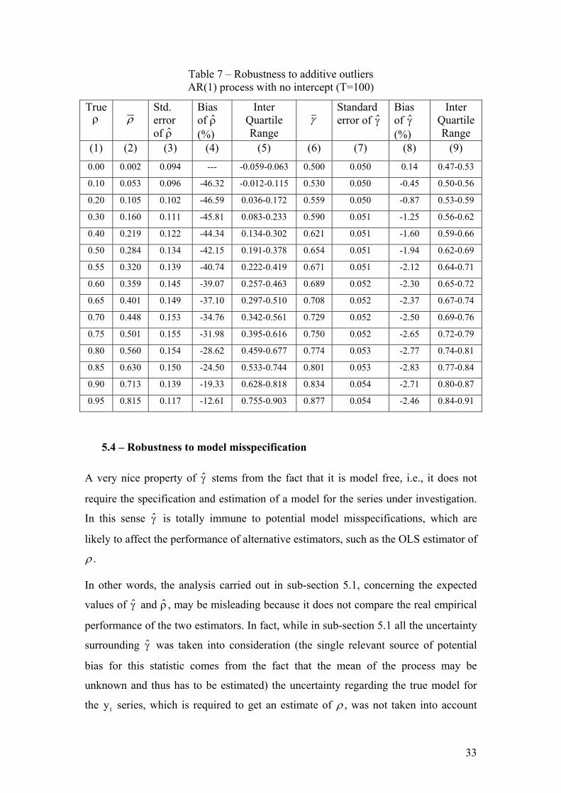
Table 7 – Robustness to additive outliers AR(1) process with no intercept (T=100)

True ρ

ρ

Std. error of $ρ

Bias of ρ $(%)

Inter Quartile Range

γ

Standard error of $γ

Bias of $γ (%)

Inter Quartile Range

(1) (2) (3) (4) (5) (6) (7) (8) (9) 0.00 0.002 0.094 --- -0.059-0.063 0.500 0.050 0.14 0.47-0.53

0.10 0.053 0.096 -46.32 -0.012-0.115 0.530 0.050 -0.45 0.50-0.56

0.20 0.105 0.102 -46.59 0.036-0.172 0.559 0.050 -0.87 0.53-0.59

0.30 0.160 0.111 -45.81 0.083-0.233 0.590 0.051 -1.25 0.56-0.62

0.40 0.219 0.122 -44.34 0.134-0.302 0.621 0.051 -1.60 0.59-0.66

0.50 0.284 0.134 -42.15 0.191-0.378 0.654 0.051 -1.94 0.62-0.69

0.55 0.320 0.139 -40.74 0.222-0.419 0.671 0.051 -2.12 0.64-0.71

0.60 0.359 0.145 -39.07 0.257-0.463 0.689 0.052 -2.30 0.65-0.72

0.65 0.401 0.149 -37.10 0.297-0.510 0.708 0.052 -2.37 0.67-0.74

0.70 0.448 0.153 -34.76 0.342-0.561 0.729 0.052 -2.50 0.69-0.76

0.75 0.501 0.155 -31.98 0.395-0.616 0.750 0.052 -2.65 0.72-0.79

0.80 0.560 0.154 -28.62 0.459-0.677 0.774 0.053 -2.77 0.74-0.81

0.85 0.630 0.150 -24.50 0.533-0.744 0.801 0.053 -2.83 0.77-0.84

0.90 0.713 0.139 -19.33 0.628-0.818 0.834 0.054 -2.71 0.80-0.87

0.95 0.815 0.117 -12.61 0.755-0.903 0.877 0.054 -2.46 0.84-0.91

5.4 – Robustness to model misspecification

A very nice property of $γ stems from the fact that it is model free, i.e., it does not

require the specification and estimation of a model for the series under investigation.

In this sense $γ is totally immune to potential model misspecifications, which are

likely to affect the performance of alternative estimators, such as the OLS estimator of

ρ .

In other words, the analysis carried out in sub-section 5.1, concerning the expected

values of $γ and ρ , may be misleading because it does not compare the real empirical

performance of the two estimators. In fact, while in sub-section 5.1 all the uncertainty

surrounding

$

$γ was taken into consideration (the single relevant source of potential

bias for this statistic comes from the fact that the mean of the process may be

unknown and thus has to be estimated) the uncertainty regarding the true model for

the series, which is required to get an estimate of yt ρ , was not taken into account

33

when evaluating the performance of $ρ . Thus, in order to get a real picture on the

relative performance of the two estimators we need, in addition, to evaluate the

performance of ρ to potential model misspecifications. $

t + ε

$

For that purpose we define a Monte Carlo experiment that exactly matches the one

analysed in sub-section 5.1 for the AR(2) model with an intercept and ρ ρ .

The unique relevant difference is that now we assume that the DGP, including the

mean of the series, is unknown, as we want to compare the behaviour of ρ and

1 2 0 8+ = .

$ $γ

under such circumstances.

Table 8 reports three alternative estimates of ρ , each corresponding to a different

estimated model. Column (2) reports the average value of $ρ when the AR(1) model

t is estimated (y yt = + −α ρ 1 ρa1 ) while column (5) reports the average value of $ρ

when a searching procedure is carried out starting with the AR(4) model with an

intercept and selecting the final model using the Schwarz criterion (ρ ). Column (4)

reports the proportion of times that the true AR(2) model is selected by the Schwarz

criterion. Finally column (7) reports the average estimated

sw

$ρ when an AR(4) is fitted

to the data (ρ ). Thus, in Table 8 we are considering the effect on the OLS estimators

of omitting relevant variables (columns (2) and (3)), introducing irrelevant variables

(columns (7) and (8)) or following a searching procedure based on the Schwarz

criterion (columns (5) and (6)).

a 4

We are interested in comparing the output in Table 8 with the output in Table 5

(columns (4) and (5)), where it was assumed that the DGP was known. The bias

reported in Table 8 is the total bias, which includes the pure bias of the OLS estimator

(Table 5, column (5)) as well as the bias stemming from model misspecification.

As regards the γ statistic, the relevant figures are those of Table 5 (columns (8) and

(9)) as the single relevant source of potential bias for this statistic comes from the fact

that the mean is unknown.

Column (3) in Table 8 reports the omitted variable bias of the OLS estimators when

an AR(1) model is estimated. Interestingly enough we see that the sign of the bias is

not always negative as in Table 5. The omitted variable bias of the OLS estimators is

positive for models (1) to (9) and negative (adding to the OLS pure bias) for models

(10) to (18). As expected the omitted variable bias increases as the true model gets

34

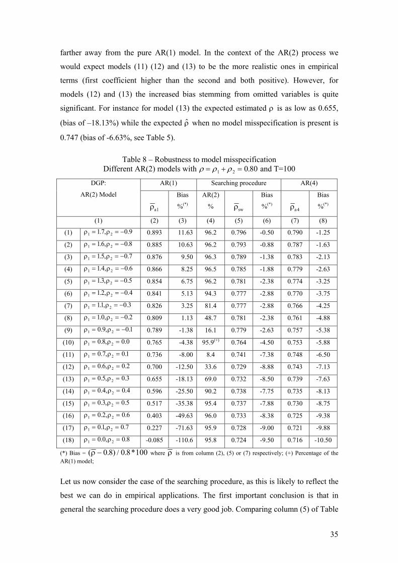
farther away from the pure AR(1) model. In the context of the AR(2) process we

would expect models (11) (12) and (13) to be the more realistic ones in empirical

terms (first coefficient higher than the second and both positive). However, for

models (12) and (13) the increased bias stemming from omitted variables is quite

significant. For instance for model (13) the expected estimated ρ is as low as 0.655,

(bias of –18.13%) while the expected $ρ when no model misspecification is present is

0.747 (bias of -6.63%, see Table 5).

Table 8 – Robustness to model misspecification Different AR(2) models with ρ ρ ρ= + =1 2 0 80. and T=100

AR(1) Searching procedure AR(4) DGP:

AR(2) Model

ρa1

Bias

%(*)

AR(2)

%

ρsw

Bias

%(*)

ρa 4

Bias

%(*)

(1) (2) (3) (4) (5) (6) (7) (8)

(1) ρ ρ1 21 7 0 9= = −. , . 0.893 11.63 96.2 0.796 -0.50 0.790 -1.25

(2) ρ ρ1 21 6 0 8= = −. , . 0.885 10.63 96.2 0.793 -0.88 0.787 -1.63

(3) ρ ρ1 21 5 0 7= = −. , . 0.876 9.50 96.3 0.789 -1.38 0.783 -2.13

(4) ρ ρ1 21= = 0 6−.4, . 0.866 8.25 96.5 0.785 -1.88 0.779 -2.63

(5) ρ ρ1 213 0 5= = −. , . 0.854 6.75 96.2 0.781 -2.38 0.774 -3.25

(6) ρ ρ1 21 2 0= = −. , .4 0.841 5.13 94.3 0.777 -2.88 0.770 -3.75

(7) ρ ρ1 211 0 3= = −. , . 0.826 3.25 81.4 0.777 -2.88 0.766 -4.25

(8) ρ ρ1 21 0 0 2= = −. , . 0.809 1.13 48.7 0.781 -2.38 0.761 -4.88

(9) ρ ρ1 20 9 0 1= = −. , . 0.789 -1.38 16.1 0.779 -2.63 0.757 -5.38

(10) ρ ρ1 20 8 0 0= =. , . 0.765 -4.38 95.9(+) 0.764 -4.50 0.753 -5.88

(11) ρ ρ1 20 7 0 1= =. , . 0.736 -8.00 8.4 0.741 -7.38 0.748 -6.50

(12) ρ ρ1 20 6 0 2= =. , . 0.700 -12.50 33.6 0.729 -8.88 0.743 -7.13

(13) ρ ρ1 20 5 0 3= =. , . 0.655 -18.13 69.0 0.732 -8.50 0.739 -7.63

(14) ρ ρ1 20 0= =.4, .4 0.596 -25.50 90.2 0.738 -7.75 0.735 -8.13

(15) ρ ρ1 20 3 0 5= =. , . 0.517 -35.38 95.4 0.737 -7.88 0.730 -8.75

(16) ρ ρ1 20 2 0 6= =. , . 0.403 -49.63 96.0 0.733 -8.38 0.725 -9.38

(17) ρ ρ1 20 1 0 7= =. , . 0.227 -71.63 95.9 0.728 -9.00 0.721 -9.88

(18) ρ ρ1 20 0 0 8= =. , . -0.085 -110.6 95.8 0.724 -9.50 0.716 -10.50

(*) Bias = ( . where ρ is from column (2), (5) or (7) respectively; (+) Percentage of the AR(1) model;

) / . *ρ − 0 8 0 8 100

Let us now consider the case of the searching procedure, as this is likely to reflect the

best we can do in empirical applications. The first important conclusion is that in

general the searching procedure does a very good job. Comparing column (5) of Table

35

8 with column (5) of Table 5 it is seen that for the bulk of the (18) models, and despite

the fact that the true AR(2) is not chosen 100% of the times, the searching procedure

ensures that the final bias of ρ does not significantly differ from the bias we get in

Table 5, i.e., under the assumption that the DGP is known. Curiously enough, the

exceptions are models (11), (12) and (13) which, as we have seen, are expected to be

the most realistic ones in empirical terms. For these three models the searching

procedure does not prevent an additional mean bias of accruing to the original bias, so

that the total bias is now between –7.0% and –9.0%. The reason is that the Schwarz

criterion picks out the AR(1) model (the wrong model) in a large proportion of times

and this implies carrying to column (6) some of the bias found in column (2).

$

As regards the effect of including irrelevant variables it is seen that there is a small

increase in the downward bias of $ρ when we compare column (8) in Table 8 with

column (5) in Table 5, so that in general there seems to be some potential gain in

implementing the searching procedure. However, it turns out that for models (11),

(12) and (13) just estimating the AR(4) model appears as a better strategy than

carrying out the general to specific methodology, based on the Schwarz criterion.

We note that the exercise in this sub-section was designed in order to deliver the best

possible results for ρ . In particular, the fact that the data are generated by an

autoregressive process (rather than an Arma model, for example) or that the

“searching procedure” or the “general model” approach are designed so that they

encompass the true DGP are examples of those favourable designing characteristics of

the exercise. In practice, it is important to bear in mind that the DGP may not be an

autoregressive model (or not be well approximated by an autoregressive model) or

that our “general estimated model” may not encompass the true model if the number

of included lags is not large enough. And, in this latter case, the “omitted variable

bias” would pop into our estimator through the back door.

$

On the other hand, it has been argued in the literature (see Schwert (1987)) that there

are many good reasons to believe that most economic time series contain moving

average components, i.e., are better described by an Arma model rather than by a pure

autoregressive process. As we have seen in section 2, assuming that the data are

described by an Arma model has the implication that ρ (the sum of autoregressive

coefficients) ceases to be the parameter of interest as it no longer measures persistence

36

of the series. The solution, in empirical terms, implies using a finite order

autoregressive process to approximate the true Arma model, but this is likely to

introduce additional biases into the estimator $ρ . In strong contrast, γ as a measure of

persistence, may be defined and its estimator, $γ , may be computed directly from the

data, irrespective of the underlying DGP.

An interesting question is whether using the “median unbiased estimator” for ρ (see

Andrews, 1994 and Hansen, 1999) allows overcoming the limitations of the OLS

estimator, , identified in this section. Resorting to the median unbiased estimator

helps alleviating the biases examined in sub-section 5.1, i.e., the biases stemming

exclusively from the OLS estimators under the assumption of correct model

specification. But, such an estimator does not seem capable of avoiding the biases

stemming from the presence of outliers or from model misspecification because it is

obtained from Monte Carlo simulations under the assumption of correct model

specification and/or distributions of the residuals without outliers.

$ρ

6. CONCLUSIONS

This paper investigates the use of mean reversion as a measure of persistence. The

distinction between the theoretical concept of mean reversion denoted by γ and its

estimator, denoted by $γ , suggested in Marques (2004), is made clear. The theoretical

properties of the estimator $γ are discussed under very general conditions and the

relationship between γ and ρ , the “sum of the autoregressive coefficients”, is

investigated. Using evidence from Monte Carlo simulations, the finite sample

properties of $γ are compared to the properties of the OLS estimator of ρ the “sum of

the autoregressive coefficients”.

Several results emerge from the paper. First, the process of obtaining the theoretical

value of γ for a general process is derived where γ is the unconditional probability of

a given process not crossing its mean, or equivalently, one minus the probability of

mean reversion of the process.

Second, it is shown that, under very general conditions, $γ is an unbiased estimator of

γ when the mean of the process is known and a consistent estimator of γ when the

mean is unknown. Moreover, it is also shown that, under the same very general

37

conditions, $γ is asymptotically normal distributed, so that tests of hypotheses on γ

can be performed very easily.

$γ

ρ2

$γ

Third, using Monte Carlo simulations for the AR(1) and AR(2) processes with normal

innovations it is shown that while the OLS estimator of ρ , $ρ , is downward biased,

is an unbiased estimator when it is assumed that the mean of the process is known.

Both estimators are downward biased when the mean of the process is unknown but

the biases of $γ are always smaller than those of $ρ . Moreover, for the AR(2) process

the biases of $ρ depend not only on the value of ρ , but also on the specific

combination of ρ1 and ρ2 , for a constant ρ .

Fourth, the same Monte Carlo simulations show that the finite sample distribution of $γ is well approximated by the normal distribution while, as expected, the distribution

of $ρ is not.

Fifth, it is shown that $ρ may be subject to significant biases coming from the presence

of additive outliers in the data or from model misspecifications, but that $γ is almost

not affected by the first potential source of bias and is, by definition, totally immune

to the second.

Finally, it is shown that there is a monotonic relationship between ρ and γ (and

several other measures of persistence) when the data is generated by an AR(1)

process, but that such a monotonic relation ceases to exist for higher order process. In

particular, it is shown for the AR(2) process with a fixed ρ that the set of measures of

persistence considered in the paper (including γ , the half-life, the largest

autoregressive root, the number of periods required for 99 percent of the adjustment to

take place) behave independently of ρ , with some of them increasing and others

decreasing as we change the combination of the autoregressive coefficients ρ1 and ,

for a constant ρ . We argue in the paper that when γ and ρ give conflicting

information about the degree of persistence it is γ and not ρ that delivers the more

important message about persistence. Notwithstanding, for higher order processes,

using γ and ρ as two companion scalar measures of persistence appears as the best

strategy given that the two measures simultaneously may allow uncovering important

features of inflation persistence that cannot be extracted from each measure alone.

Specifically, values of ρ clearly above to what could be expected given the value of $

38

can be seen as signalling the presence of a cyclical behaviour in the model of inflation

(which the central bank may not find as particularly worrisome as this implies that

inflation would cross the inflation target more frequently than could be suggested by

the value of ρ) while estimates of $ ρ clearly below to the ones we would expect given

the estimated γ may be signalling strong downward biases of the OLS (or the median

unbiased) estimator of ρ , stemming from the presence of additive outliers in the data

or from model misspecification.

7. REFERENCES

Andrews, Donald W.K., 1991, “Heteroskedasticity and autocorrelation consistent

covariance matrix estimation”, Econometrica, Vol.59, No. 3, 817-858;

Andrews, Donald W.K., 1993, “Exactly median unbiased estimation of first order

autoregressive/unit root models”, Econometrica, Vol.61, No. 1, 139-165;

Andrews Donald W. K., Chen, Hong-Yuan, 1994, “Approximately median-unbiased

estimation of autoregressive models”, Journal of Business and Economic

Statistics, Vol. 12, No. 2, 187- 204;

Burridge P., Guerre E., 1996, “The limit distribution of level crossings of a random

walk, and a simple unit root test”, Econometric Theory, 12, 705-723;

den Haan W. J, Levin A. T., 1997, “A practitioner’s guide to robust covariance matrix

estimation”, in G. S. Maddala and C. J. Rao, ed., Handbook of Statistics,

Amsterdam: Elsevier;

Evans, G. B. A., Savin, N. E., 1981, “Testing for unit roots”, Econometrica, Vol. 49,

No.3, 753-779;

Gadzinski G., Orlandi, F., 2004, “Inflation persistence for the EU countries the euro

area and the US”, mimeo.

Hamilton, James D., 1994, Time series analysis, Princeton University Press;

Hansen, Bruce E., 1999, “The grid bootstrap and the autoregressive model”, The

review of Economics and Statistics, Vol. 81, No. 4, 594-607;

Lucas, André, 1995, “An outlier robust unit root test with an application to the extend

Nelson-Plosser data”, Journal of Econometrics, Vol. 66, 153-173;

Marques, Carlos Robalo, 2004, “Inflation persistence: facts or artefacts?”, ECB

Working Paper No. 371;

39

Murray C. J., Papell, D. H., 2002, “The purchasing power parity persistence

paradigm”, Journal of International Economics, 56, 1-19;

Phillips, P. C. B., 1977, “Approximations to some finite sample distributions

associated with a first-order stochastic difference equation”, Econometrica,

No. 2, 463-485;

Pivetta F., Reis, R., 2001, “The persistence of inflation in the United States”, mimeo;

Politis, D., N., White, H., 2004, “Automatic block-length selection for the dependent

bootstrap”, Econometric Reviews, Vol. 23, No.1, 53-70;

Sawa, T., 1978, “The exact moments of the least squares estimator for the

autoregressive model”, Journal of Econometrics, 8, 159-172;

Schwert, G., W., 1987, “Effects of model specification on tests for unit roots in

macroeconomic data”, Journal of Monetary Economics, 20, 73-103;

Spanos, A., 1990, Statistical foundations of econometric modelling, Cambridge

University Press;

Stock, J., 1991, “Confidence intervals for the largest autoregressive root in the US

macroeconomic time series”, Journal of Monetary Economics, 28, 435-459;

Stock, J., 2001, “Comment”, NBER, Macroeconomics Annula, edited by Ben S.

Bernanke and Kenneth Rogoff;

White, H., 1984, Asymptotic Theory for Econometricians, Academic Press;

40

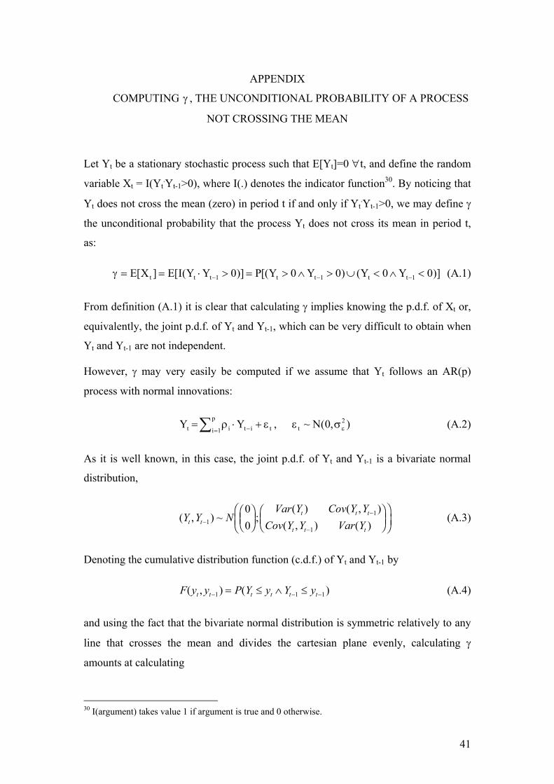
APPENDIX

COMPUTING γ , THE UNCONDITIONAL PROBABILITY OF A PROCESS

NOT CROSSING THE MEAN

Let Yt be a stationary stochastic process such that E[Yt]=0 ∀t, and define the random

variable Xt = I(Yt.Yt-1>0), where I(.) denotes the indicator function30. By noticing that

Yt does not cross the mean (zero) in period t if and only if Yt.Yt-1>0, we may define γ

the unconditional probability that the process Yt does not cross its mean in period t,

as:

γ = = ⋅ > = > ∧ > ∪ < ∧ <− −E X E I Y Y P Y Y Y Yt t t t t t t[ ] [ ( )] [( ) ( )1 10 0 0 0 0− ]1 (A.1)

From definition (A.1) it is clear that calculating γ implies knowing the p.d.f. of Xt or,

equivalently, the joint p.d.f. of Yt and Yt-1, which can be very difficult to obtain when

Yt and Yt-1 are not independent.

However, γ may very easily be computed if we assume that Yt follows an AR(p)

process with normal innovations:

Y Y Nt i t ii

pt t= ⋅ +−=∑ ρ ε ε ε1

20, ~ ( , σ ) (A.2)

As it is well known, in this case, the joint p.d.f. of Yt and Yt-1 is a bivariate normal

distribution,

( , ) ~ ;( ) ( , )

( , ) ( )Y Y N

Var Y Cov Y YCov Y Y Var Yt t

t t t

t t t−

−

−

FHGIKJFHG

IKJ

FHG

IKJ1

1

1

00

(A.3)

Denoting the cumulative distribution function (c.d.f.) of Yt and Yt-1 by

F y y P Y y Y yt t t t t t( , ) ( )− −= −≤ ∧ ≤1 1 1

(A.4)

and using the fact that the bivariate normal distribution is symmetric relatively to any

line that crosses the mean and divides the cartesian plane evenly, calculating γ

amounts at calculating

30 I(argument) takes value 1 if argument is true and 0 otherwise.

41

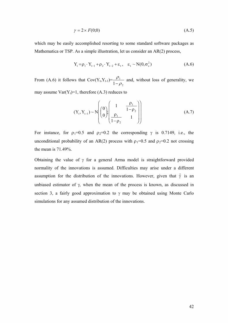
γ = ×2 0F( ; )0 (A.5)

which may be easily accomplished resorting to some standard software packages as

Mathematica or TSP. As a simple illustration, let us consider an AR(2) process,

Y Y Y Nt t t t t= ⋅ + ⋅ +− −ρ ρ ε ε σε1 1 2 220, ~ ( , ) (A.6)

From (A.6) it follows that Cov(Yt,Yt-1)=ρρ1

21− and, without loss of generality, we

may assume Var(Yt)=1, therefore (A.3) reduces to

( , ) ~ ;Y Y Nt t−FHGIKJ

−

−

F

H

GGG

I

K

JJJ

F

H

GGG

I

K

JJJ1

1

2

1

2

00

11

11

ρρ

ρρ

(A.7)

For instance, for ρ1=0.5 and ρ2=0.2 the corresponding γ is 0.7149, i.e., the

unconditional probability of an AR(2) process with ρ1=0.5 and ρ2=0.2 not crossing

the mean is 71.49%.

Obtaining the value of γ for a general Arma model is straightforward provided

normality of the innovations is assumed. Difficulties may arise under a different

assumption for the distribution of the innovations. However, given that $γ is an

unbiased estimator of γ, when the mean of the process is known, as discussed in

section 3, a fairly good approximation to γ may be obtained using Monte Carlo

simulations for any assumed distribution of the innovations.

42

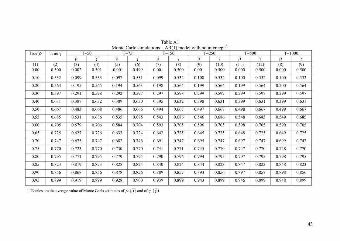
Table A1 Monte Carlo simulations – AR(1) model with no intercept(*)

T=50 T=75 T=150 T=250 T=500 T=1000True ρ True γ ρ γ ρ γ ρ γ ρ γ ρ γ ρ γ

(1) (2) (3) (4) (5) (6) (7) (8) (9) (10) (11) (12) (8) (9)0.00 0.500 0.002 0.501 -0.001 0.499 0.001 0.500 0.001 0.500 0.000 0.500 0.000 0.500

0.10 0.532 0.099 0.533 0.097 0.531 0.099 0.532 0.100 0.532 0.100 0.532 0.100 0.532

0.20 0.564 0.195 0.565 0.194 0.563 0.198 0.564 0.199 0.564 0.199 0.564 0.200 0.564

0.30 0.597 0.291 0.598 0.292 0.597 0.297 0.598 0.299 0.597 0.299 0.597 0.299 0.597

0.40 0.631 0.387 0.632 0.389 0.630 0.395 0.632 0.398 0.631 0.399 0.631 0.399 0.631

0.50 0.667 0.483 0.668 0.486 0.666 0.494 0.667 0.497 0.667 0.498 0.667 0.499 0.667

0.55 0.685 0.531 0.686 0.535 0.685 0.543 0.686 0.546 0.686 0.548 0.685 0.549 0.685

0.60 0.705 0.579 0.706 0.584 0.704 0.593 0.705 0.596 0.705 0.598 0.705 0.599 0.705

0.65 0.725 0.627 0.726 0.633 0.724 0.642 0.725 0.645 0.725 0.648 0.725 0.649 0.725

0.70 0.747 0.675 0.747 0.682 0.746 0.691 0.747 0.695 0.747 0.697 0.747 0.699 0.747

0.75 0.770 0.723 0.770 0.730 0.770 0.741 0.771 0.745 0.770 0.747 0.770 0.748 0.770

0.80 0.795 0.771 0.795 0.779 0.795 0.790 0.796 0.794 0.795 0.797 0.795 0.798 0.795

0.85 0.823 0.819 0.823 0.828 0.824 0.840 0.824 0.844 0.823 0.847 0.823 0.848 0.823

0.90 0.856 0.868 0.856 0.878 0.856 0.889 0.857 0.893 0.856 0.897 0.857 0.898 0.856

0.95 0.899 0.919 0.899 0.928 0.900 0.939 0.899 0.943 0.899 0.946 0.899 0.948 0.899

(*) Entries are the average value of Monte Carlo estimates of ρ (ρ ) and of γ (γ ).

43

Table A2 Monte Carlo simulations – AR(1) model with an intercept(*)

T=50 T=75 T=150 T=250 T=500 T=1000True ρ True γ ρ γ ρ γ ρ γ ρ γ ρ γ ρ γ

(1) (2) (3) (4) (5) (6) (7) (8) (9) (10) (11) (12) (8) (9)0.00 0.500 -0.018 0.495 -0.014 0.494 -0.006 0.498 -0.003 0.499 -0.002 0.499 -0.001 0.500

0.10 0.532 0.077 0.526 0.082 0.526 0.092 0.530 0.096 0.531 0.098 0.531 0.099 0.531

0.20 0.564 0.171 0.557 0.178 0.558 0.190 0.562 0.195 0.563 0.197 0.563 0.198 0.564

0.30 0.597 0.264 0.589 0.274 0.590 0.288 0.595 0.293 0.596 0.296 0.596 0.298 0.597

0.40 0.631 0.358 0.622 0.370 0.624 0.386 0.629 0.392 0.629 0.396 0.630 0.398 0.630

0.50 0.667 0.452 0.656 0.466 0.658 0.484 0.663 0.491 0.665 0.495 0.665 0.498 0.666

0.55 0.685 0.499 0.674 0.514 0.677 0.533 0.682 0.540 0.683 0.545 0.684 0.547 0.685

0.60 0.705 0.545 0.692 0.562 0.696 0.582 0.701 0.589 0.702 0.595 0.703 0.597 0.704

0.65 0.725 0.591 0.711 0.609 0.715 0.631 0.721 0.639 0.722 0.644 0.724 0.647 0.724

0.70 0.747 0.638 0.731 0.657 0.736 0.680 0.742 0.688 0.744 0.694 0.745 0.697 0.746

0.75 0.770 0.684 0.753 0.705 0.758 0.729 0.765 0.737 0.767 0.744 0.768 0.747 0.769

0.80 0.795 0.730 0.775 0.752 0.782 0.777 0.789 0.787 0.791 0.793 0.793 0.797 0.794

0.85 0.823 0.775 0.800 0.800 0.807 0.826 0.816 0.836 0.819 0.843 0.821 0.846 0.822

0.90 0.856 0.819 0.826 0.846 0.837 0.875 0.848 0.885 0.851 0.893 0.854 0.896 0.855

0.95 0.899 0.862 0.854 0.891 0.869 0.922 0.885 0.934 0.891 0.942 0.895 0.946 0.897

(*) Entries are the average value of Monte Carlo estimates of ρ (ρ ) and of γ (γ ).

44

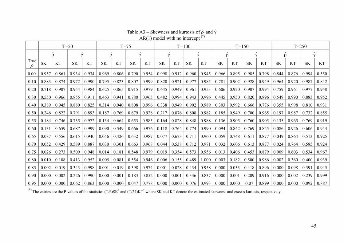
Table A3 – Skewness and kurtosis of $ρ and $γ AR(1) model with no intercept (*)

T=50 T=75 T=100 T=150 T=250

$ρ $γ $ρ $γ $ρ $γ $ρ $γ $ρ $γ True ρ SK KT SK KT SK KT SK KT SK KT SK KT SK KT SK KT SK KT SK KT

0.00 0.957 0.861 0.934 0.934 0.969 0.806 0.790 0.954 0.998 0.912 0.960 0.945 0.966 0.895 0.985 0.798 0.844 0.876 0.994 0.550

0.10 0.883 0.874 0.972 0.990 0.795 0.823 0.807 0.999 0.820 0.921 0.977 0.985 0.781 0.902 0.928 0.949 0.964 0.920 0.987 0.842

0.20 0.718 0.907 0.954 0.984 0.625 0.865 0.915 0.979 0.645 0.949 0.961 0.953 0.606 0.920 0.907 0.994 0.759 0.961 0.977 0.958

0.30 0.550 0.966 0.855 0.911 0.463 0.941 0.780 0.965 0.482 0.994 0.943 0.996 0.445 0.950 0.820 0.896 0.549 0.990 0.883 0.952

0.40 0.389 0.945 0.880 0.825 0.314 0.940 0.808 0.996 0.338 0.949 0.902 0.989 0.303 0.992 0.666 0.776 0.355 0.998 0.810 0.931

0.50 0.246 0.822 0.791 0.893 0.187 0.769 0.679 0.928 0.217 0.876 0.808 0.982 0.185 0.949 0.700 0.965 0.197 0.987 0.732 0.855

0.55 0.136 0.184 0.746 0.735 0.972 0.134 0.664 0.653 0.985 0.164 0.828 0.848 0.988 0.905 0.760 0.905 0.135 0.965 0.769 0.919

0.60 0.131 0.659 0.687 0.999 0.090 0.549 0.666 0.976 0.118 0.764 0.774 0.990 0.094 0.842 0.769 0.825 0.086 0.926 0.606 0.944

0.65 0.087 0.556 0.615 0.940 0.056 0.426 0.632 0.987 0.077 0.673 0.711 0.960 0.059 0.748 0.611 0.877 0.049 0.864 0.513 0.925

0.70 0.052 0.429 0.589 0.887 0.030 0.301 0.663 0.968 0.044 0.538 0.712 0.971 0.032 0.606 0.613 0.877 0.024 0.764 0.585 0.924

0.75 0.026 0.273 0.509 0.948 0.014 0.181 0.548 0.979 0.019 0.354 0.573 0.956 0.013 0.406 0.453 0.879 0.009 0.603 0.534 0.967

0.80 0.010 0.108 0.413 0.952 0.005 0.081 0.554 0.946 0.006 0.155 0.489 1.000 0.003 0.182 0.500 0.986 0.002 0.360 0.400 0.939

0.85 0.002 0.019 0.343 0.998 0.001 0.019 0.398 0.974 0.001 0.028 0.434 0.958 0.000 0.033 0.418 0.896 0.000 0.098 0.391 0.945

0.90 0.000 0.002 0.226 0.990 0.000 0.001 0.183 0.852 0.000 0.001 0.336 0.837 0.000 0.001 0.209 0.916 0.000 0.002 0.239 0.999

0.95 0.000 0.000 0.062 0.863 0.000 0.000 0.047 0.778 0.000 0.000 0.076 0.993 0.000 0.000 0.07 0.899 0.000 0.000 0.092 0.887(*) The entries are the P-values of the statistics (T/6)SK2 and (T/24)KT2 where SK and KT denote the estimated skewness and excess kurtosis, respectively.

45

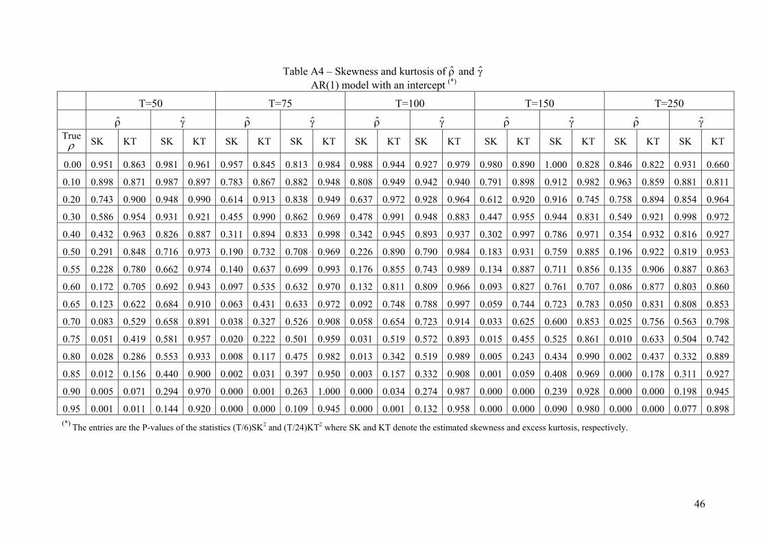
Table A4 – Skewness and kurtosis of $ρ and $γ AR(1) model with an intercept (*)

T=50 T=75 T=100 T=150 T=250

$ρ $γ $ρ $γ $ρ $γ $ρ $γ $ρ $γ True ρ SK KT SK KT SK KT SK KT SK KT SK KT SK KT SK KT SK KT SK KT

0.00 0.951 0.863 0.981 0.961 0.957 0.845 0.813 0.984 0.988 0.944 0.927 0.979 0.980 0.890 1.000 0.828 0.846 0.822 0.931 0.660

0.10 0.898 0.871 0.987 0.897 0.783 0.867 0.882 0.948 0.808 0.949 0.942 0.940 0.791 0.898 0.912 0.982 0.963 0.859 0.881 0.811

0.20 0.743 0.900 0.948 0.990 0.614 0.913 0.838 0.949 0.637 0.972 0.928 0.964 0.612 0.920 0.916 0.745 0.758 0.894 0.854 0.964

0.30 0.586 0.954 0.931 0.921 0.455 0.990 0.862 0.969 0.478 0.991 0.948 0.883 0.447 0.955 0.944 0.831 0.549 0.921 0.998 0.972

0.40 0.432 0.963 0.826 0.887 0.311 0.894 0.833 0.998 0.342 0.945 0.893 0.937 0.302 0.997 0.786 0.971 0.354 0.932 0.816 0.927

0.50 0.291 0.848 0.716 0.973 0.190 0.732 0.708 0.969 0.226 0.890 0.790 0.984 0.183 0.931 0.759 0.885 0.196 0.922 0.819 0.953

0.55 0.228 0.780 0.662 0.974 0.140 0.637 0.699 0.993 0.176 0.855 0.743 0.989 0.134 0.887 0.711 0.856 0.135 0.906 0.887 0.863

0.60 0.172 0.705 0.692 0.943 0.097 0.535 0.632 0.970 0.132 0.811 0.809 0.966 0.093 0.827 0.761 0.707 0.086 0.877 0.803 0.860

0.65 0.123 0.622 0.684 0.910 0.063 0.431 0.633 0.972 0.092 0.748 0.788 0.997 0.059 0.744 0.723 0.783 0.050 0.831 0.808 0.853

0.70 0.083 0.529 0.658 0.891 0.038 0.327 0.526 0.908 0.058 0.654 0.723 0.914 0.033 0.625 0.600 0.853 0.025 0.756 0.563 0.798

0.75 0.051 0.419 0.581 0.957 0.020 0.222 0.501 0.959 0.031 0.519 0.572 0.893 0.015 0.455 0.525 0.861 0.010 0.633 0.504 0.742

0.80 0.028 0.286 0.553 0.933 0.008 0.117 0.475 0.982 0.013 0.342 0.519 0.989 0.005 0.243 0.434 0.990 0.002 0.437 0.332 0.889

0.85 0.012 0.156 0.440 0.900 0.002 0.031 0.397 0.950 0.003 0.157 0.332 0.908 0.001 0.059 0.408 0.969 0.000 0.178 0.311 0.927

0.90 0.005 0.071 0.294 0.970 0.000 0.001 0.263 1.000 0.000 0.034 0.274 0.987 0.000 0.000 0.239 0.928 0.000 0.000 0.198 0.945

0.95 0.001 0.011 0.144 0.920 0.000 0.000 0.109 0.945 0.000 0.001 0.132 0.958 0.000 0.000 0.090 0.980 0.000 0.000 0.077 0.898(*) The entries are the P-values of the statistics (T/6)SK2 and (T/24)KT2 where SK and KT denote the estimated skewness and excess kurtosis, respectively.

46

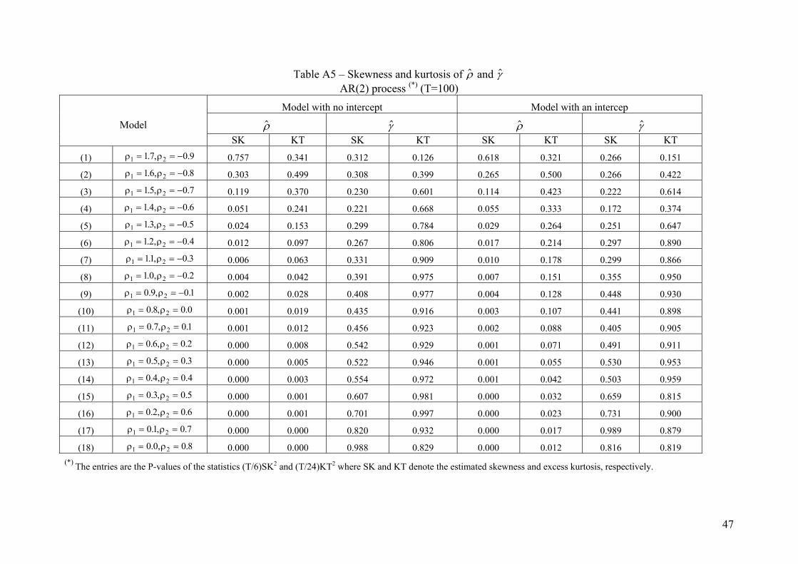
47

Table A5 – Skewness and kurtosis of $ρ and $γ AR(2) process (*) (T=100)

Model with no intercept Model with an intercep

$ρ $γ $ρ $γ

Model SK KT SK KT SK KT SK KT

(1) ρ ρ1 21 7 0 9= = −. , . 0.757 0.341 0.312 0.126 0.618 0.321 0.266 0.151

(2) ρ ρ1 21 6 0 8= = −. , . 0.303 0.499 0.308 0.399 0.265 0.500 0.266 0.422

(3) ρ ρ1 21 5 0 7= = −. , . 0.119 0.370 0.230 0.601 0.114 0.423 0.222 0.614

(4) ρ ρ1 21 0 6= = −.4, . 0.051 0.241 0.221 0.668 0.055 0.333 0.172 0.374

(5) ρ ρ1 213 0 5= = −. , . 0.024 0.153 0.299 0.784 0.029 0.264 0.251 0.647

(6) ρ ρ1 21 2 0= = −. , .4 0.012 0.097 0.267 0.806 0.017 0.214 0.297 0.890

(7) ρ ρ1 211 0 3= = −. , . 0.006 0.063 0.331 0.909 0.010 0.178 0.299 0.866

(8) ρ ρ1 21 0 0 2= = −. , . 0.004 0.042 0.391 0.975 0.007 0.151 0.355 0.950

(9) ρ ρ1 20 9 0 1= = −. , . 0.002 0.028 0.408 0.977 0.004 0.128 0.448 0.930

(10) ρ ρ1 20 8 0 0= =. , . 0.001 0.019 0.435 0.916 0.003 0.107 0.441 0.898

(11) ρ ρ1 20 7 0 1= =. , . 0.001 0.012 0.456 0.923 0.002 0.088 0.405 0.905

(12) ρ ρ1 20 6 0 2= =. , . 0.000 0.008 0.542 0.929 0.001 0.071 0.491 0.911

(13) ρ ρ1 20 5 0 3= =. , . 0.000 0.005 0.522 0.946 0.001 0.055 0.530 0.953

(14) ρ ρ1 20 0= =.4, .4 0.000 0.003 0.554 0.972 0.001 0.042 0.503 0.959

(15) ρ ρ1 20 3 0 5= =. , . 0.000 0.001 0.607 0.981 0.000 0.032 0.659 0.815

(16) ρ ρ1 20 2 0 6= =. , . 0.000 0.001 0.701 0.997 0.000 0.023 0.731 0.900

(17) ρ ρ1 20 1 0 7= =. , . 0.000 0.000 0.820 0.932 0.000 0.017 0.989 0.879

(18) ρ ρ1 20 0 0 8= =. , . 0.000 0.000 0.988 0.829 0.000 0.012 0.816 0.819(*) The entries are the P-values of the statistics (T/6)SK2 and (T/24)KT2 where SK and KT denote the estimated skewness and excess kurtosis, respectively.