using machine learning to predict the number of

International Journal of Industrial Optimization Vol. 2, No. 1, February 2021, pp. 1-16

P-ISSN 2714-6006 E-ISSN 2723-3022

Emerick et al

1

Using machine learning to predict the number of alternative

solutions to a minimum cardinality set covering problem

Brooks Emerick, Yun Lu, Francis J. Vasko*

Department of Mathematics, Kutztown University, Kutztown, USA

[email protected]; [email protected]; [email protected]

*Corresponding Authors: [email protected]

1. Introduction

Characterizing and determining alternative optimal solutions to linear programming problems is a

standard topic in operations research textbooks (Hillier & Lieberman, 2010; Taha, 2017).

However, the literature on alternative optimal solutions for combinatorial optimization problems,

especially NP-hard combinatorial optimization problems, is virtually non-existent. The only paper

the authors are aware of is by Huang et al. (2018), which tries to find multiple solutions for the

traveling salesman problem by incorporating a genetic algorithm into a niching technique. Papers

that come close to characterizing alternative optimal solutions do not deal with NP-hard problems.

For example, Hamacher & Queyranne (1985) developed an algorithm based on a binary search

tree procedure to find the K best bases in a matroid, perfect matchings, and best cuts in a network.

ARTICLE INFO

ABSTRACT

Keywords Minimum cardinality set covering problem; Unicost set covering problem; Machine learning; Regression trees; Number of alternative optimal solution.

Although the characterization of alternative optimal solutions for

linear programming problems is well known, such

characterizations for combinatorial optimization problems are

essentially non-existent. This is the first article to qualitatively

predict the number of alternative optima for a classic NP-hard

combinatorial optimization problem, namely, the minimum

cardinality (also called unicost) set covering problem (MCSCP).

For the MCSCP, a set must be covered by a minimum number of

subsets selected from a specified collection of subsets of the given

set. The MCSCP has numerous industrial applications that require

that a secondary objective is optimized once the size of a minimum

cover has been determined. To optimize the secondary objective,

the number of MCSCP solutions is optimized. In this article, for the

first time, a machine learning methodology is presented to

generate categorical regression trees to predict, qualitatively

(extra-small, small, medium, large, or extra-large), the number of

solutions to an MCSCP. Within the machine learning toolbox of

MATLAB®, 600,000 unique random MCSCPs were generated and

used to construct regression trees. The prediction quality of these

regression trees was tested on 5000 different MCSCPs. For the 5-

output model, the average accuracy of being at most one off from

the predicted category was 94.2%.

Article history Received: October 15, 2020 Revised: January 3, 2021 Accepted: January 15, 2021

Available online: February 24, 2021

International Journal of Industrial Optimization

Vol. 2, No.1, February 2021, pp. 1-16 P-ISSN 2714-6006 E-ISSN 2723-3022

Emerick et al. 2

Lawler (19720 presented a system for computing the 𝐾 best solutions to discrete optimization

problems and then applied it to the shortest path problem. To the authors’ knowledge, there are

no procedures presented in the literature for either quantitatively or qualitatively predicting how

many alternative optimal solutions there are for any combinatorial optimization problem. This is

the first article to develop a methodology for predicting qualitatively the number of alternative

optimal solutions to an NP-hard combinatorial optimization problem, namely, the minimum

cardinality set covering problem (MCSCP). The mathematical formulation of the MCSCP will now

be given.

Let 𝐴 = [𝑎𝑖𝑗] be an 𝑚 × 𝑛 matrix, where 𝑚 < 𝑛, and the entries of 𝐴 are zeros and ones.

Suppose the row and column sum of the matrix 𝐴 is at least one. We seek the solution to the

minimum cardinality set covering problem (MCSCP), which is formulated as follows: Let 𝑥 = [𝑥𝑗]

be an 𝑛 × 1 column vector of ones and zeros only (𝑥 is a bit string), then

{

Minimize: ∑𝑥𝑗

𝑛

𝑗=1

(1)

Constraint: ∑𝑎𝑖𝑗𝑥𝑗

𝑛

𝑗=1

for 𝑖 = 1, 2,⋯ ,𝑚 (2)

For any matrix A that meets the above conditions, there is at least one solution to the MCSCP,

which implies that the solution vector x may not be unique. In this article, the focus is on answering

the following question: Given the matrix 𝐴 with known density of ones, can the number of

alternative solution vectors 𝑥 with the same minimum cardinality be confidently predicted?

Although the minimum cardinality set covering problem (MCSCP) is NP-hard (Karp, 1972),

with recent improvements in integer programming software (Bixby, 2012) it is now possible to

determine optimal solutions to some “larger” MCSCPs in a reasonable amount of time. Hence,

some industrial applications involving MCSCPs can be solved exactly. Furthermore, there are

essential industrial applications that are essentially pre-emptive goal programs in which the first

goal is to solve an MCSCP and then, given the MCSCP solution, find an optimal solution to a

secondary objective. Two such examples from the steel industry are optimal ingot mold selection

(Vasko et al., 1987) and metallurgical grade assignment (Vasko et al., 1989). For ingot mold

selection, the first priority is to minimize the number of mold sizes because the inventory

investment, material-handling, and logistical considerations associated with an additional mold

size outweigh the potential yield or productivity benefits from increasing the number of mold sizes.

Similar arguments can be made to keep the number of metallurgical grades assigned to customer

orders to a minimum. For these applications, knowing, at least qualitatively, the number of

alternative optimal MCSCP solutions could help determine the appropriate approach to use when

solving the optimum value of the secondary objective (yield loss for ingot mold selection and

material costs grade assignment).

The authors were familiar with the work of Vasko et al. (2005) in which regression tree analysis

was used to qualitatively predict if coal blends would be good or bad for coke oven processes and

blast furnace operations. There were four possible outcomes: bad coke oven-bad blast furnace

impact, bad coke oven-good blast furnace impact, good coke oven-bad blast furnace impact, and



Emerick et al. 3

good coke oven-good blast furnace impact. For the candidate coal blend to receive further

consideration, the regression tree model predicted that its use would result in a good coke oven

and good blast furnace impact. Furthermore, Saleh et al. (2018) successfully used artificial neural

networks (ANN), which is considered a subset of machine learning, to predict CO2 emissions.

Additionally, Williams et al. (2009) used ANNs in MATLAB to successfully solve a mass

spectrometry application. Given these successful applications, the authors decided to use the

Statistical and Machine Learning Toolbox function fitter in MATLAB to generate regression trees

to predict the number of alternative optimal solutions to MCSCPs qualitatively.

This paper is organized as follows: In Section 2 we present our methodology, which consists

of statistical analysis on a representative set of MCSCPs, the construction of regression trees

trained from this set, and the validation of the regression trees on a test set of MCSCPs; in Section

3, we discuss the implications and limitations of our results; and we close with concluding remarks

in Section 4.

2. Research Methodology

To qualitatively predict the number of alternative solutions to a given MCSCP, we use a

methodology based on machine learning. We study the characteristics of a large sample of

MCSCPs to identify relevant attributes of a particular problem that may suggest a number of

alternative solutions to that problem. Because a single MCSCP is completely determined by the

constraint matrix 𝐴, we randomly generate 600,000 matrices in MATLAB to act as a representative

sample. Each matrix was unique with a fixed size and density of ones. Specifically, each matrix

𝐴 = [𝑎𝑖𝑗] has 𝑚 = 10 rows, 𝑛 = 20 columns, and 𝑝 = 20% density of ones. It is an initial study,

and we hope to adapt our results to various sizes and thicknesses in the future. Below, we

describe our methods for statistically analyzing this representative sample of MCSCPs. Then, we

describe how the sample is used as a training set to generate several categorical regression

trees, which are then used to predict the number of alternative optima of any given MCSCP.

2.1 . Statistical Analysis

We seek a frequency distribution of the number of alternative optimal solutions for each of the

600,000 MCSCPs. To this end, we solve each MCSCP using the intlinprog function of MATLAB.

Then, we use a brute force method to enumerate all alternative solutions. For example, if the

minimum cardinality of an MCSCP is 4, then we search through all 𝐶20 4 sets of columns of size 4

to determine if that set is indeed a solution. Given the number of alternative solutions for each

MCSCP, the purpose of the analysis is to identify specific characteristics of the matrix 𝐴 that

correspond to a higher or lower number of alternative solutions.

The descriptive statistics for the number of optimal solutions for the 600,000 MCSCPs is given

in Table 1. The table provides the mean, standard deviation, and the five-number summary of the

entire data set. The data set has a strong right skew. Table 1 indicates that the minimum number

of optimal solutions is one, which means a matrix yields a unique solution. The maximum number

of alternative solutions is 672. The table shows the outlier threshold, which is the maximum

number of optimal solutions not considered an outlier. In this case, if a matrix has greater than or

equal to 36 optimal solutions, then it is considered an outlier relative to the data set.



Emerick et al. 4

Table 1. Summary statistics for the number of optimal solutions of the global data set of MCSCPs

Mean Std. Dev. Five-Number Summary Outlier

Threshold

Proportion

in 𝑼𝒎𝒊𝒏

Proportion

in 𝑼𝒎𝒂𝒙 Min 𝑸𝑳 M 𝑸𝑳 Max

13.79 20.62 1 2 6 15.5 672 35.75 14.93% 10.31%

An MCSCP (matrix) is defined to have an unusually large number of solutions if the number of

solutions is an outlier, i.e., exceeds the value of 35.75. There are 61,846 (10.31%) MCSCPs with

an unusually large number of solutions, and so these MCSCPs are denoted as 𝑈𝑚𝑎𝑥. The set

𝑈𝑚𝑖𝑛 is defined as the set of all MCSCPs with exactly one optimal solution. There are precisely

89,604 MCSCPs (14.93%) with a unique solution vector of the entire data set.

For each of the 600,000 MCSCPs, the goal was to identify important (relevant to the number

of alternative solutions) characteristics of the corresponding 𝐴 matrix. Observe that the minimum

cardinality and the number of alternative solutions is invariant under row or column swapping.

Figure 1 shows a matrix 𝐴 with minimum cardinality of 5 in its original form and in its sorted form,

where a blue dot represents a one, and the rest of the elements are zero. To obtain this sorted

form, the rows are first sorted by the first non-zero element that appears. A secondary sort is

applied such that the columns are sorted by descending column sum with a tiebreaker being

determined by the smallest row with a nonzero entry. Furthermore, the matrix in Figure 1 has a

unique solution, which is shown as the five highlighted columns.

In the sorted form, several defining attributes of the matrix 𝐴 are characteristic of other matrices

within the set 𝑈𝑚𝑖𝑛. The matrix A, which has a unique solution, in its original form (top) and in its

sorted form (bottom). A blue dot represents a one, the rest of the matrix entries are zero. The five

red columns show the solution to the MCSCP, which contains the five columns contained in the

set covering. For example, in Figure 1, it should be noted that rows 4, 8, and 10 contain a single

element. Because of this, all solution vectors must contain columns 4, 15, and 20. Therefore, this

matrix will have a smaller number of optimal solutions simply because three of the five possible

columns in a solution must be columns 4, 15, and 20. In short, the number of possible optimal

solutions has been reduced from 𝐶20 5 = 15504 to 𝐶17

2 = 136. This is a 99% reduction. Thus, the

number of rows of the matrix 𝐴 that contain a single element is a matrix characteristic of interest

to this analysis. Furthermore, it should be noted that column 4 also has only a single element. In

contrast, columns 15 and 20 contain other elements that may contribute in some way to a

covering. Because column 4 must be in the solution, but it doesn't “help” with a covering, this

matrix is said to have an isolated point. Hence, the number of isolated points in any matrix is also

a characteristic of interest to this analysis.

Using the sorted version of each matrix as a visual guide, we compute descriptive statistics for

other attributes about matrices' samples. Table 2 compares a few other defining characteristics

of the matrices with a unique solution (the set 𝑈𝑚𝑖𝑛) to the matrices with an unusually large number

of solutions (the set 𝑈𝑚𝑎𝑥). The average and standard deviation of the measures for each set are

compared. In addition to the number of single element rows and isolated points, the number of

duplicate columns, the number of dominated and dominating columns, the proportion of nonzero

elements in the matrix 𝐴𝐴𝑇, the number of elements in each quadrant of the sorted matrix and



Emerick et al. 5

some statistical measures about the row sum and column sum is computed. In total, 26

characteristics are considered as the set of decision variables for the regression tree.

Figure 1. The matrix 𝐴

1 2 3 4 5 6 7 8 9 10 11 12 13 14 15 16 17 18 19 20

Column Number

1

2

3

4

5

6

7

8

9

10

Ro

w N

um

be

r

Original Matrix with Solution

1 2 3 4 5 6 7 8 9 10 11 12 13 14 15 16 17 18 19 20

Column Number

1

2

3

4

5

6

7

8

9

10

Ro

w N

um

be

r

Sorted Matrix with Solution



Emerick et al. 6

Table 2. A comparison of matrix characteristics from the set of all matrices

The bolded entries in the table represent the variables that yield the top five largest 𝑡-statistics

for a difference of means significance test. To clarify, most of the means (for each decision

variable) are significantly different between the sets 𝑈𝑚𝑖𝑛 and 𝑈𝑚𝑎𝑥. The bolded entries reflect the

Decision Variable Notation Mean/STD of 𝑼𝒎𝒊𝒏 Mean/STD of 𝑼𝒎𝒂𝒙

Minimum Cardinality 𝑚 3.58/0.51 5.01/0.25

Dominated Columns 𝑥1 10.64/1.76 10.21/1.62

Dominating Columns 𝑥2 12.97/1.07 12.79/1.16

Single Element Rows 𝑥3 0.64/0.69 0.42/0.57

Maximum Column Sum of Single

Element Row 𝑥4 1.44/1.61 1.01/1.42

Isolated Points 𝑥5 0.10/0.31 0.06/0.24

Duplicate Columns 𝑥6 2.56/1.22 2.52/1.22

Rows with Maximum Row Sum 𝑥7 1.45/0.81 1.44/0.78

Proportion of Nonzero Elements in

𝐴𝐴𝑇 𝑥8 0.52/0.06 0.48/0.05

Maximum Eigenvalue of 𝐴𝐴𝑇 𝑥9 12.53/1.15 12.45/1.15

Elements in Northwest Quadrant 𝑥10 12.03/2.35 12.25/2.39

Elements in Northeast Quadrant 𝑥11 7.97/2.18 7.74/2.14

Elements in Southwest Quadrant 𝑥12 4.99/2.35 5.13/2.24

Elements in Southeast Quadrant 𝑥13 15.01/1.78 14.88/1.89

Mean of Row Sum 𝑥14 4.00/0.00 4.00/0.00

Standard Deviation of Row Sum 𝑥15 1.74/0.39 1.70/0.34

Median of Row Sum 𝑥16 3.91/0.38 3.87/0.37

Interquartile Range of Row Sum 𝑥17 1.82/0.86 1.76/0.80

Minimum of Row Sum 𝑥18 1.52/0.59 1.65/0.55

Maximum of Row Sum 𝑥19 6.91/1.03 6.89/0.98

Mean of Column Sum 𝑥20 2.00/0.00 2.00/0.00

Standard Deviation of Column Sum 𝑥21 1.02/0.16 0.95/0.14

Median of Column Sum 𝑥22 1.95/0.18 1.98/0.10

Interquartile Range of Column Sum 𝑥23 1.60/0.46 1.54/0.54

Minimum of Column Sum 𝑥24 1.00/0.00 1.00/0.00

Maximum of Column Sum 𝑥25 4.29/0.75 4.02/0.65



Emerick et al. 7

decision variables that yield the five smallest 𝑝-values when comparing means between the two

groups. The minimum cardinality (𝑚), the number of single element rows (𝑥3), the proportion of

nonzero entries in 𝐴𝐴𝑇(𝑥8), the standard deviation of column sum (𝑥21), and the max column sum

(𝑥25) are among the most statistically different variables between the two sets 𝑈𝑚𝑖𝑛 and 𝑈𝑚𝑎𝑥.

Minimum cardinality is a strong factor for determining the number of alternative solutions.

Figure 2 compares the number of alternative optimal solutions for each cardinality using a series

of boxplots. The red crosses denote outliers in the respective set of matrices for each cardinality.

The number of solutions has a strong right skew for each cardinality. The majority of the matrices

with minimum cardinality of three have less than five solutions with a maximum of 24.

In contrast, matrices with minimum cardinality of five or six can contain solutions in the

hundreds. In all cases, however, at least one unique solution is attained for all minimum

cardinalities. It provides insight into the fact that minimum cardinality will be an important predictor

variable in determining the number of alternative solutions.

Figure 2. A series of boxplots for each set of optimal solutions according to minimum cardinality

2.2. Regression Tree Analysis

Categorical Regression Trees were constructed using the built-in fitctree function in MATLAB

from the Statistical and Machine Learning Toolbox. This function will create a regression decision

tree trained from each of the matrices corresponding to the 600,000 MCSCPs. Each input to

construct a tree will consist of a matrix with attributes from Table 2. These variables will act as

standard classification and regression trees (CART) predictor variables. The algorithm selects the

split predictor that maximizes the Gini diversity index (GDI) that gain over all other predictors'

possible splits to choose the best split predictor variable at each node. Once the tree is formed,

0 5 10 15 20 25

Min

-Ca

rd 3

0 20 40 60 80 100

Min

-Ca

rd 4

50 100 150 200 250 300

Min

-Ca

rd 5

0 100 200 300 400 500 600 700

Min

-Ca

rd 6

Number of Optimal Solutions

Boxplot of Optimal Solutions for Each Minimum Cardinality



Emerick et al. 8

the output consists of the number of solutions defined as a small, medium or large version. The

algorithm creates an estimated optimal sequence of subtrees as it is growing the classification

tree. In this sense, the tree can be “pruned” to contain a smaller number of nodal splits according

to this optimal sequence. The subtrees are based on maximizing the GDI index at each stage

(MATLAB, 2020). The tree is pruned to have the minimum number of branches such that all types

of solution categories are present. We considered two regression trees with a different number

of output categories.

We create two models based on the number of outputs: a 3-output model with small (𝑆),

medium (𝑀), and large (𝐿) number of alternative solutions and a 5-output model with 𝑋𝑆, 𝑆, 𝑀, 𝐿,

𝑋𝐿, where 𝑋𝑆 denotes extra small and 𝑋𝐿 represents the extra-large number of alternative

solutions. The discrete cutoff values for each category are determined by the criteria defined in

Table 3. The interval definitions are presented in interval notation. For example, the 3-output

regression tree outputs a 𝑆 if the tree predicts the number of solutions to be less than 6, an 𝑀 if

the number of solutions is predicted to be between 6 and 36, and 𝐿 if the number of solutions is

36 or more. Similarly, in the 5-output regression tree, an 𝑋𝑆 is for a unique solution, 𝑆 is for

solutions between 2 and 6, 𝑀 is for solutions between 6 and 16, 𝐿 is between 16 and 36, and 𝑋𝐿

is beyond 36 solutions.

Table 3. Interval definitions for the categories associated to 𝑆, 𝑀, and 𝐿 for the 3-output regression trees

and the categories associated to 𝑋𝑆, 𝑆, 𝑀, 𝐿, and 𝑋𝐿, for the 5-output regression trees

3-Output Tree 5-Output Tree

𝑆 𝑀 𝐿 𝑋𝑆 𝑆 𝑀 𝐿 𝑋𝐿

[1,6) [6,36) [36,672] [1,2) [2,6) [6,16) [16,36) [36,672]

Two unique regression trees are trained using the set of 600,000 matrices with all 26 predictor

variables from Table 2. The unpruned regression trees each have the maximum number of

branches allowed by MATLAB – 9,999 branches. The unpruned trees are not shown. These two

regression trees are tested on the original data set to determine the success rate. The regression

trees were pruned to have the smallest number of branch points while still maintaining every

possible categorical output. The pruning technique is based on the estimated optimal sequence

of subtrees. The pruned trees each have only three branches and are shown in Figure 3.

It is interesting to note the success rates for the pruned trees as well as the number of branches

on the pruned trees. The unpruned trees do perform undeniably much better than the pruned

trees. This is likely because the unpruned trees have a total of 26 predictor variables to help make

an informed decision on whether to split into a different category or not. However, we see that

there are only three branches for each of the 3-output and 5-output trees with the most important

predictor variables being the number of single element rows (𝑥3) and the proportion of nonzero

entries in the matrix 𝐴𝐴𝑇 (𝑥8). The proportion of nonzero elements in 𝐴𝐴𝑇 (𝑥8) is a measure of

how compatible any two columns are at covering a particular row. Indeed, if 𝑥8 is closer to 1, then

there likely exists two columns that potentially cover identical rows, thus allowing for more

alternative solutions. We note that the minimum cardinality determines the initial split. The

matrix's minimum cardinality clearly distinguishes two cohorts: a smaller set of alternative



Emerick et al. 9

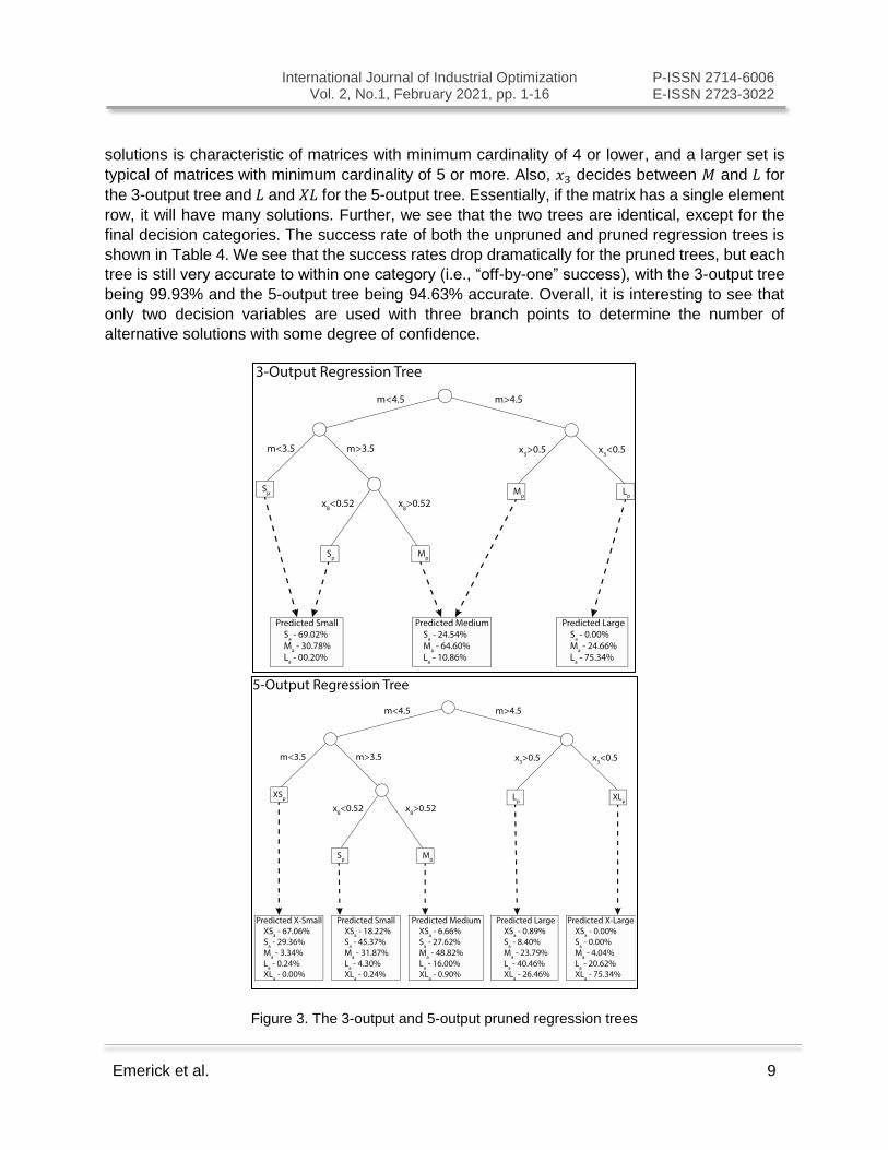
solutions is characteristic of matrices with minimum cardinality of 4 or lower, and a larger set is

typical of matrices with minimum cardinality of 5 or more. Also, 𝑥3 decides between 𝑀 and 𝐿 for

the 3-output tree and 𝐿 and 𝑋𝐿 for the 5-output tree. Essentially, if the matrix has a single element

row, it will have many solutions. Further, we see that the two trees are identical, except for the

final decision categories. The success rate of both the unpruned and pruned regression trees is

shown in Table 4. We see that the success rates drop dramatically for the pruned trees, but each

tree is still very accurate to within one category (i.e., “off-by-one” success), with the 3-output tree

being 99.93% and the 5-output tree being 94.63% accurate. Overall, it is interesting to see that

only two decision variables are used with three branch points to determine the number of

alternative solutions with some degree of confidence.

Figure 3. The 3-output and 5-output pruned regression trees



Emerick et al. 10

Table 4. The success rate of the two regression trees

Not Pruned Pruned

Success “Off-by-One” Success “Off-by-One” Branches

3-Output Tree 91.50% 99.94% 68.59% 99.93% 3

5-Output Tree 84.09% 96.97% 50.29% 94.63% 3

2.3. Validation

The two regression tree models were tested on a set of randomly generated matrices. Specifically,

5,000 matrices unique from the original set of 600,000 matrices used to train the regression tree

were used to validate the two regression trees. Tables 5 and 6 show a detailed analysis of each

tree's success rate for each category. For example, for the 3-output tree, the numbers in the cell

labeled as actually small (denoted by the event 𝑆𝑎) and predicted small (denoted by the event 𝑆𝑝)

indicated that 1,751 of the 5,000 test matrices (35.02%) were predicted to be small by the tree

and they were small. However, 781 matrices were predicted to be small, but they were medium.

Considering the matrix of values, it is clear that the tree is 99.90% accurate to within one category

because the only time the tree's prediction was more than one category removed was for the 5

times that the tree predicted small, but they were actually large (top right cell of the table).

Table 5. The frequencies and relative frequencies of MCSCPs that were actually 𝑆/𝑀/𝐿 and predicted to

be 𝑆/𝑀/𝐿 by the pruned 3-output tree on the validation set of 5,000 MCSCPs.

3-Output Tree

Actual

Total 𝑆𝑎 𝑀𝑎 𝐿𝑎

Pre

dic

ted

𝑆𝑝 1751 (35.02%) 781 (15.62%) 5 (0.10%) 2537 (50.74%)

𝑀𝑝 495 (9.90%) 1303 (26.06%) 219 (4.38%) 2017 (40.34%)

𝐿𝑝 0 (0%) 110 (2.20%) 336 (6.72%) 446 (8.92%)

Total 2246 (44.92%) 2194 (43.88%) 560 (11.20%) 5000 (100%)



Emerick et al. 11

Table 6. The frequencies and relative frequencies of MCSCPs that were actually 𝑋𝑆/𝑆/𝑀/𝐿/𝑋𝐿 and

predicted to be 𝑋𝑆/𝑆/𝑀/𝐿/𝑋𝐿 by the pruned 5-output tree on the validation set of 5,000 MCSCPs.

5-Output Tree

Actual

𝑋𝑆𝑎 𝑆𝑎 𝑀𝑎 𝐿𝑎 𝑋𝐿𝑎 Total

Pre

dic

ted

𝑿𝑺𝒑 281

(5.62%)

123

(2.46%) 14 (0.28%) 1 (0.02%) 0 (0%) 419 (8.38%)

𝑆𝑝 386

(7.72%)

961

(19.22%)

675

(13.50%)

91

(1.82%) 5 (0.10%) 2118 (42.36%)

𝑀𝑝 82

(1.64%)

340

(6.80%)

601

(12.02%)

197

(3.94%)

11

(0.22%) 1231 (24.62%)

𝐿𝑝 7 (0.14%) 66

(1.32%)

187

(3.74%)

318

(6.36%)

208

(4.16%) 786 (15.72%)

𝑋𝐿𝑝 0 (0%) 0 (0%) 18 (0.36%) 92

(1.84%)

336

(6.72%) 446 (8.92%)

Total

756

(15.12%)

1490

(29.80%)

1495

(29.90%)

699

(13.98%)

560

(11.20%) 5000 (100%)

5-Output Tree

Actual

𝑋𝑆𝑎 𝑆𝑎 𝑀𝑎 𝐿𝑎 𝑋𝐿𝑎 Total

Pre

dic

ted

𝑿𝑺𝒑 281

(5.62%)

123

(2.46%) 14 (0.28%) 1 (0.02%) 0 (0%) 419 (8.38%)

𝑆𝑝 386

(7.72%)

961

(19.22%)

675

(13.50%)

91

(1.82%) 5 (0.10%) 2118 (42.36%)

𝑀𝑝 82

(1.64%)

340

(6.80%)

601

(12.02%)

197

(3.94%)

11

(0.22%) 1231 (24.62%)

𝐿𝑝 7 (0.14%) 66

(1.32%)

187

(3.74%)

318

(6.36%)

208

(4.16%) 786 (15.72%)

𝑋𝐿𝑝 0 (0%) 0 (0%) 18 (0.36%) 92

(1.84%)

336

(6.72%) 446 (8.92%)

Total

756

(15.12%)

1490

(29.80%)

1495

(29.90%)

699

(13.98%)

560

(11.20%) 5000 (100%)



Emerick et al. 12

Using this information, the 3-output and 5-output regression trees are presented in Figure 3

with the final decision, including weighted percentages of the tree's misreading. Conditionally, for

the 5-output model, if we know the tree has predicted extra-large, there is a 75.34% chance

(based on this simulation of 5,000 random matrices) that the matrix actually has an extra-large

number of alternative solutions, i.e.,

𝑃(𝑋𝐿𝑎 | 𝑋𝐿𝑝) = 336

0 + 0 + 18 + 92 + 336= 75.34%.

We may also define the “off-by-one” conditional probability of success. For instance, let 𝐿�̃�

denote the event that the MCSCP is within one category of large, i.e., it either has medium, large,

or extra-large alternative optima. The, we may calculate the following probability to indicate that

if the 5-output model predicts a large number of solutions, then we can be 90.71% confident that

the actual number of solutions is within one category of being large, based on this set of 5,000

test matrices.

𝑃(𝐿�̃� | 𝐿𝑝) = 187 + 318 + 208

7 + 66 + 187 + 318 + 208= 90.71%

3. Results and Discussion

Our preceding analysis yields several important results that shed light on the idea of predicting

the number of alternative solutions to the MCSCP. The statistical work conducted above on a set

of 600,000 randomized MCSCPs gives insight into the distribution of alternative optima. Our

representative sample found that the majority, 90.04%, of MCSCPs of size 10 × 20 with 20%

density of ones has a minimum cardinality of 4 or 5. For the whole representative sample, we find

that the distribution of the number of alternative solutions is severely skewed, with 13.76 being

the average number of alternative optima with a maximum number of 672. An MCSCP is

considered an outlier relative to the data if it has greater than 35 alternative optima. Approximately

10% of the data are outliers, and approximately 15% of MCSCPs considered have a unique

solution. Given the data, every outlier has a minimum cardinality of at least 4. It indicates that

minimum cardinality is a reliable determinant of a larger number of alternative optima, resulting

from our regression tree analysis. Our set of 600,000 matrices, although only a small proportion

of the possible problems of size 10 × 20, illustrates the nature of how alternative optima arise in

MCSCPs. Constructing the population of all MCSCPs of this size is unfathomable, and thus our

statistical approach using a randomized sample of a decent size provides a first look into the

nature of these problems.

The two pruned regression trees, presented in Figure 3, help to predict, at least qualitatively,

the number of alternative optima for any given MCSCP. The unpruned trees perform

extraordinarily well on the original training set, but they have an unreasonable number of

branches. Therefore, they would likely not be used in practice. The pruned trees still perform quite

well with only three branches and provide insight into the most important characteristics of the

MCSCP. Indeed, the decision nodes determined by the regression tree algorithm indicate that

minimum cardinality (𝑚), the number of single element rows (𝑥3), and the proportion of non-zeros

in the matrix 𝐴𝐴𝑇 (𝑥8) have the most impact. Given any MCSCP, these three numerical values

are not difficult to compute and yet, based on our analysis, should give a reasonable prediction



Emerick et al. 13

about the number of alternative optima. We find that if the minimum cardinality is greater than 4,

then it is probable that the MCSCP has a medium, large, or extra-large number of optimal

solutions. In the 3-output model, this means that the MCSCP has at least 6 alternatives optimal.

Using the 5-output model, this means the problem has at least 16 alternative optima. In any case,

we can conclude that if the minimum cardinality is more than 4, the problem likely does not have

a unique solution. In contrast, our models show that if the minimal cardinality is less than 3, the

MCSCP probably has less than 5 alternative solutions.

A more in-depth look into our regression trees show that the variables 𝑥3 and 𝑥8 are the

deciding factors in the second phase of the algorithm. Indeed, the number of single-row elements

typically determines the difference between medium and large or large and extra-large for the 3-

output and 5-output models, respectively. This is a reasonable result because if an MCSCP has

a larger minimal cardinality, the number of solutions will only increase if there are less “isolated”

points. Interestingly, we find that if a matrix has one or more single element row, then this will

significantly change the number of alternative solutions. According to both models, if the matrix

has zero single element rows, it is likely an outlier (in the sense of alternative optima). Likewise,

if the proportion of nonzero elements of 𝐴𝐴𝑇is less than 0.52, then the problem likely has a small

number of solutions rather than a medium number. Of the 26 possible decision variables

considered, we find that only these two are the most important for determining more subtle

differences in the number of alternative optima.

We validated the two regression trees on a unique set of 5,000 MCSCPs. The preliminary

results of the validation are shown in Figures 5 and 6. Using the validation, we can provide more

insight into our models' success and assign probabilities to possible outcomes. Although the

pruned trees do not effectively predict exact matches on the original training set (68.59% for 3-

output and 50.29% for 5-output), we find that the pruned models do perform well for predicting

the number of solutions to within one category (99.93% for 3-Output and 94.63% for 5-output).

On the validation set, we see that both models perform best when predicting exact matches for

large optima numbers. That is, 𝑃(𝐿𝑎| 𝐿𝑝) = 75.34% for the 3-output model and 𝑃(𝑋𝐿𝑎| 𝑋𝐿𝑝) =

75.34% for the 5-output model. The 3-output model manages to maintain more than 60%

accuracy for exact small and medium predictions. If we relax the definition of success and

consider correct predictions within one category (i.e., “off-by-one” success), we see that both

models reach at least 90%. Indeed, using the output from Table 6, we may compute the

conditional probabilities in Table 7, which show the performance of the 5-output regression tree

in determining the number of optimal solutions to within one category. In this case, the average

success rate is 94.20%, which indicates that the 5-output is successful in predicting, at least

qualitatively, the number of alternative optima of a MCSCP.

Table 7. The performance of the 5-output tree in predicting the correct number of alternative solutions

Conditional Probability “Off-by-One” Success

𝑃(𝑋𝑆𝑎 |̃ 𝑋𝑆𝑝) 96.42%

𝑃(𝑆𝑎 |̃ 𝑆𝑝) 95.48%

𝑃(𝑀𝑎 |̃ 𝑀𝑝) 92.45%

𝑃(𝐿𝑎 |̃ 𝐿𝑝) 90.71%

𝑃(𝑋𝐿𝑎 |̃ 𝑋𝐿𝑝) 95.96%



Emerick et al. 14

Our present analysis uses the minimum cardinality (𝑚) as an input variable to train the

regression tree. It comes as no surprise that this variable is the most important in determining

each tree's initial decision node. To isolate this variable, we also created regression trees within

each minimum cardinality (not shown). We found that not only were 𝑥3 and 𝑥8 important variables

within each cardinality, but also the standard deviation of the row sum (𝑥15). We see similar

accuracies for regression trees within each minimum cardinality.

4. Conclusion

The present study's goal was to qualitatively predict the number of alternative optima for a classic

NP-hard combinatorial optimization problem such as the MCSCP. To the authors’ knowledge, this

article is the first attempt to answer this question. Aside from being an interesting theoretical

question, the answer to this question has potential practical implications. Our methods to

randomly generate matrices corresponding to 600,000 MCSCPs were analyzed using the

machine learning function of MATLAB®. Twenty-six matrix characteristics were identified as

potentially relevant for this analysis and used as input to generate categorical regression trees.

There were two regression trees generated: a 3-output tree and a 5-output tree. The 3-output tree

predicted either a small, medium, or large number of solutions for an MCSCP, and the 5-output

tree predicted either an extra small, small, medium, large, or extra-large number of solutions for

an MCSCP. The prediction quality of these trees was determined using a separate set of 5,000

MCSCPs. The trees were most accurate in predicting a large number (3-output) of optimal

solutions and an extra-large number (5-output) of optimal solutions. We find that both models are

particularly accurate in predicting whether an MCSCP has a large number of solutions based on

only three, easily calculable characteristics of the constraint matrix. Indeed, the 5-output model

can essentially predict the nature of the number of alternative optima within one category with a

success rate of 94.20%, on average.

The significance of this study is observed in the potential applications it has to real-world

problems. One specific application is that of ingot mold selection (Vasko et al., 1987). The goal of

such a study is to determine the minimum number of ingot mold sizes. Once the minimum number

of ingot mold sizes is found, the secondary objective is to minimize yield loss. Using our

methodology, if the application is predicted to have a small number of alternative optima, then

more effort may be required to find a near-optimal solution for the second objective function.

Alternatively, if our methodology predicts that many alternative solutions exist, then it may require

less computational effort to find a near-optimal solution for the secondary objective.

This work was a first attempt to qualitatively predict the number of optimal solutions to a

MCSCP, so our results are limited to a specific MCSCP, one that corresponds to a constraint

matrix of size 10 × 20 with 20% density of ones. Therefore, the results of this analysis may be

regarded as a pilot study for problems of this nature. Given the success obtained so far, future

work will involve using a larger variety of MCSCPs as input to generate models that qualitatively

predict the number of optimal MCSCP solutions. We seek to expand the results presented here

to problems with different densities of ones and/or larger sizes in general. We may be able to

speculate that keeping the size the same while increasing the density will yield a larger proportion

of MCSCPs with lesser minimum cardinalities, thereby decreasing the number of alternative

solutions across the board. We wish to determine specific trends in MCSCPs with varying

densities as well as with varying sizes. However, as the constraint matrix size increases, the curse



Emerick et al. 15

of dimensionality may limit our progress since searching for all optimal solutions of a specific

cardinality becomes a daunting task. Finally, we are interested in applying the methodology

discussed in this article to analyze the number of alternative optima for other combinatorial

optimization problems.

References

C. Saleh, R.A.C. Leuuveano, M.N.A. Rahman, B. M. Deros, & N.R., Dzakiyullah. (2015). Predicting of CO2 emissions using an artificial neural network: the case of the sugar industry. Adv. Sci. Lett., 21, 3079-3083.

D. K. Williams Jr., A. L. Kovach, D. C. Muddiman, & K. W. Hanck. (2009). Utilizing artificial neural networks in MATLAB to achieve parts-per-billion mass measurement accuracy with a fourier transform ion cyclotron resonance mass spectrometer. American Society for Mass Spectrometry, 20, 1301-1310.

E.L. Lawler. (1972). Procedure for computing the K best solutions to discrete optimization problems and its application to the shortest path problem. Management Science, 18(7), 401-405.

F. J. Vasko, F. E. Wolf, & K. L. Stott. (1987). Optimal selection of ingot sizes via set covering. Opns Res, 35, 346-353.

F. J. Vasko, F. E. Wolf, & K. L. Stott. (1989). A set covering approach to metallurgical grade Assignment. Eur J Opl Res, 38, 27-34.

F. J. Vasko, D. D. Newhart, & A. D. Strauss. (2005). Coal blending models for optimum cokemaking and blast furnace operation. Journal of the Operational Research Society, 56 (3), 235-243.

F. S. Hillier & J. Lieberman. (2010). Introduction to Operations Research. 9th Edition, New York: McGraw-Hill.

H.W. Hamacher & M. Queyranne, M. (1985). K-best solutions to combinatorial optimization problems. Annals of Operations research, 4, 123-145.

H. Taha. (2017). Operations Research: An Introduction, 10th Edition, Pearson, Boston, MA.

MATLAB. (2020). Statistics and Machine Learning Toolbox User’s Guide. R2020a, 1 Apple Hill Dr, Natick, MA 01760-2098.

R. E., Bixby. (2012). A brief history of linear and mixed-integer programming computation. Documenta Mathematica Extra volume ISMP, 107-121.

R. M. Karp. (1972). Reducibility among combinatorial problems,” in Complexity of Computer Computations, Miller R E and Thatcher J W (eds), 85-103. Plenum, New York.

T. Huang, Y. Gong, & J. Zhang. (2018). Seeking multiple solutions of combinatorial optimization problems: a proof of principle study”, in 2018 IEEE Symposium Series on Computational Intelligence (SSCI), 1212-1218. Bangalore, India.



Emerick et al. 16

This page is intentionally left blank.

using machine learning to predict the number of

Documents