Using Grid Benchmarks for Dynamic Scheduling of Grid Applications

Michael Frumkin, Robert Hood+ NASA Advanced Supercomputing Division

+Computer Sciences Corporation M / S T27A-2, NASA Ames Research Center

Moffett Field, CA 94035- 1 OOO {frumkin,rhood}@nas.nasa.gov

Abstract

Navigation or dynamic scheduling of applications on computational grids can be improved through the use of an application-specijic characterization of grid resources. Current grid information systems provide a description of the resources, but do not contain any application-speciJc information. We defne a “GridScape ’’ as dynamic state of the grid resources. We measure the dynamic performance of these resources using the grid benchmarks. Then we use the GridScape for automatic assignment of the tasks of a grid application to grid resources. The scalability of the system is achieved by limiting the navigation overhead to a few percent of the application resource requirements. Our task submission and assignment protocol guarantees that the navigation system does not cause grid congestion. On a synthetic data mining application we demonstrate that Gridscape-based task assignment reduces the application tunaround time.

Keywords: computational grids, benchmarks, performance, navigation, dynamic scheduling.

1 Introduction

Manual navigation’, or dynamic scheduling of applications on a grid is challenging because the grid resources are dynamic and heterogeneous. An automated navigation system would make the grid more efficient and accessible by improving application turnaround times and lowering user effort. A number of research projects have been devoted to obtaining, monitoring and forecasting the state of grid resources, and to the scheduling of individual grid resources and applications. These projects provide a suite of tools and services that can be used in a navigation system, however, the problem of congestion-free, scalable automatic navigation on the grid is still open. Moreover, crucial components of grid resource characterization, such as the number of currently available processors per grid machine or the efficiency of their use on applications, are still not available to grid users.

A navigation system considers an application as a set of communicating tasks. It makes a sequence of scheduling decisions depending on the state of the tasks and the state of grid resources and takes into account the spatial component of the grid such as latency of the communications. Scheduling, on the other hand is a rigid planning and assignment of known tasks to a fixed set of resources. Our approach to the automation of navigation is based on automatic characterization of the grid, extrapolating an

application’s performance profile to the relevant grid resources, and assigning tasks of the application to the best fitting

‘Navigate -to steer a course through a medium, Merrim-Webster’s Collegiate Dictionary.

https://ntrs.nasa.gov/search.jsp?R=20030032283 2018-06-01T16:34:23+00:00Z

t

I

grid resources. In [9] we have shown that this approach reduces application turnaround time. The scalability of the system is achieved by limiting the navigation overhead to a few percent of the application resource requirements.

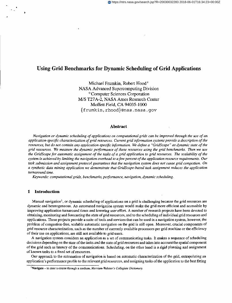
In this paper we extend this approach in two directions. First, we extend the grid mapping capabilities of the navigation system to a grid monitoring system that periodically updates grid performance information. Second, we introduce the Waiting-Assigned-Running-Executed task submission protocol. This results in a congestion-free (cf. "Bushel of AppLeS Problem" [2]) navigation system. The architecture of the system is shown in Figure 1. We describe the interaction between servers and navigators in Section 3, and the acquisition and use of the Gridscape in Section 4.

Figure 1. The Architecture of our Navigation System. Each navigator executes the iterations of the Navigational Cycle (see Figure 2). The navigators and servers follow the WARE protocol of Section 3 that guarantees that the grid does not get congested.

We demonstrate the efficiency of our navigation system on an Arithmetic Data Cube (ADC) (see [lo]). (In [9] we used W.W and MB.W of the NAS Grid Benchmarks [ l l ] as the grid applications.) The ADC is a data intensive application which generates all possible views of a data set, Section 5. In Section 6 we show that our navigation system reduces ADC turnaround time by 25%. For our experiments we extend the rudimentary grid of [9] to a grid with peak performance of 1.6 TFLOPS, which includes shared memory machines from SUN and SGI.

As an abstraction of grid resources we use a Gridscape-a map of the grid resources represented by a directed graph, where each grid machine (and router) is represented as a node of the graph with an attached list of the machine resources and a history of their dynamics. Communication links between machines are represented by the arcs of the graph, which are labeled with the observed bandwidth and latency of the links. The initial information about the Gridscape is acquired during installation of the servers (see Figure 1). The dynamic, application-specific component of the GridScape is measured by means of NAS Grid Benchmarks (NGB) (see Section 7) during the monitoring and by requests of the navigators.

We consider grid applications consisting of a number of tasks, cf. [3]. Each task obtains its input data either from its predecessors or from the launching task. It sends data either to its successors or to the reporting task. A task is ready for execution when data from all its predecessors has been delivered. As soon as the task has finished, it sends the results to all its successors. We model such applications by data flow graphs. The nodes of the graph represent tasks, and the arcs represent data flow between tasks. We assume that data flow graphs are Directed Acyclic Graphs (DAG). In some problem solving environments [ 151 it was demonstrated that distributed applications can be well-formulated in terms of data flow (or task) graphs. Grid applications built of distributed components [ 121 can often also be modeled by data flow graphs.

2

2 Related Work

Dynamic scheduling of applications is addressed in the Application Level Scheduler (AppLeS) project [2,3]. The goal of the AppLeS project is to provide mechanisms that perform selection of grid resources and scheduling of grid applications. Each AppLeS agent uses static and dynamic information about both the application and the grid to select viable resource configurations and evaluate their potential performance. AppLeS agents interact with the relevant resource management system to implement application tasks. Once an application contains an embedded AppLeS agent, it becomes self-scheduling. AppLeS templates are stand-alone software projects performing scheduling and deployment tasks for classes of structurally similar applications. AppLeS are application specific, and each application must be linked with an AppLeS agent. AppLeS does not allow the user to intervene into the scheduling process and change it at run time. The “Bushel of AppLeS” problem formulated in [2] is essentially a problem of grid congestion caused by applications competing for the best grid resources. Our navigational system follows the WARE protocol (see Section 3), which guarantees that grid resources do not get congested.

A partial map of a grid in given time intervals can be obtained with the Network Weather Service ( N W S ) . N W S measures end-to-end TCP/IP performance (bandwidth and latency), available CPU fraction, and available non-paged memory. The N W S periodically monitors and dynamically forecasts the performance that various network and com- putational resources can deliver over a given time interval. The N W S operates a distributed set of performance sensors from which it gathers readings of the instantaneous conditions. It then uses numerical models to generate forecasts of what the conditions will be for a given time frame. The performance information collected by N W S is intended for use by dynamic schedulers and to provide statistical Quality-of-Service readings in a networked computational environment. The N W S facilities are used by AppLeS, and its prototype implementation is available for Globus and the Global Grid Forum Grid Information System architecture. N W S uses the standard UNIX uptime and vmstat commands to obtain the performance of grid machines; it sends packets of data to obtain TCPm performance. It ob- tains the performance information in adjustable discrete intervals of time. N W S employs a “push” information model, where the user can obtain N W S information and forecasts; however, it provides no means to request performance tests at a specified moment on a specified subset of grid resources.

The Globus Heart Beat Monitor (HBM) [13] allows a grid user to monitor tasks of a grid application by communi- cating with one of the HBM Data Collectors (HBMDC). A number of HBMDCs monitor all tasks running on the grid, typically one per grid and one for each distributed application. Each HBMDC maintains a repository of the reports received from HBM local monitors. HBM supports the monitoring of tasks running on the grid and the tracking of their success or failure. As with the N W S , it uses a push data model.

The problem solving environment SCIRun [lS] allows the user to steer an application from start to completion by managing each step in a sequential computing process, and by creating batch processes that execute repeated simulations. SCIRun provides a data flow API and allows the user to intervene and control the execution of each node of the graph (computational steering). SCIRun provides neither the means for acquisition of map of the grid nor the automation of choice of the grid resources.

The Grid Information Protocol [7] (MDS2) provides information about grid resources and protocols to discover this information. The implementation of MDS2 is based on the LDAP protocol, which has significant latency in updating the directory and is thus more properly considered as a repository of static information about grid resources.

The recently developed Metascheduler for the Grid [20] is built on the top of the Grid Application Development Software (GrADS) architecture [5]. The Metascheduler has the ability to discover, reserve, and negotiate grid resources to insure that multiple scheduling requests will not cause grid congestion and that an application will make progress even if requested resources are currently unavailable. The Metascheduler assumes that multiple grid services are working properly.

The resource Brokering Infrastructure for Computational Grids [I] provides a job submission and monitoring mech- anism for computational grids. The system facilitates policy enforcement for various grid resources. It provides a plug-and-play framework for scheduling algorithms and grid applications. It uses the Jini technology for resource discovery. This infrastructure can be used with both Globus and Sun Grid Engine.

3

I - - I

3 The Navigational Cycle

In our navigation system the submissions of application tasks to the grid resources are made by the navigators (see Figure 1)*. The decision to accept or reject the submision is performed by a server. The navigators run on launch machines, while the servers are on grid machines.

For a given application a navigator performs the following functions:

0 obtain a list of tasks that are ready to be executed;

0 find the grid resources that are able to execute these tasks;

0 submit the tasks to the grid resources that will provide the fastest advance of the application;

0 repeat this sequence until all tasks of the application are executed.

In order for a navigator to be able to accomplish these functions, it should be able to understand an application’s requirements and to know the current state of grid resources.

In a grid environment, a list of an application’s requirements (OS, compiler, libraries, run time systems) and its performance model (the number of FLOPS, parallel efficiency, memory size, cache efficiency, size of I/O data) must be part of an application description and should be provided to the navigational system. The requirements list and the performance model may be created by a user or may be extracted from the application by an automatic analysis tool.

As an abstraction of grid resources we use the GridScape described earlier. It lists the capabilities of grid machines and the interconnections between them. When deciding to submit a task, a navigator uses a Gridscape. How to obtain a GridScape and keep it current is discussed in Section 4.

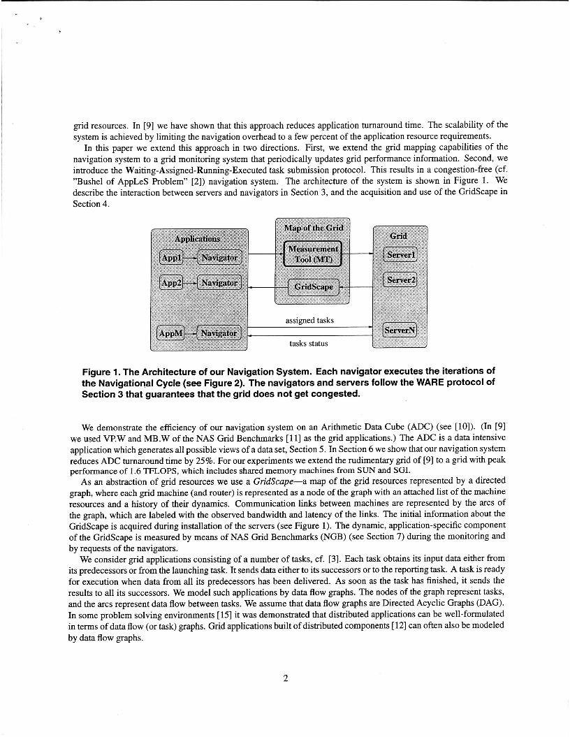
The navigator matches the task requirements with abilities of grid resources in the following three steps. First, it compares the list of the task requirements with the current abilities of the grid resources as listed in the GridScape. Second, it estimates the time it will take to execute the task on each grid resource that is able to accomplish the task. Finally, it submits the task to the resource that minimizes the application turnaround time. In summary, the navigator performs the routine of the navigational cycle shown in Figure 2.

Gridscape Application Performance Model q-

Figure 2. The Navigational Cycle. The navigator performs iterations of the navigational cycle.

Each grid machine runs one server performing the following functions:

0 check that each submitted task was submitted with use of the current Gridscape;

’In other papers on dynamic scheduting, cf. [l J they are called brokers.

4

0 accept the qualified tasks for an execution;

0 return the unqualified tasks to the navigator;

0 update the Gridscape after accepting a task and executing a task.

Navigators and servers follow the “WARE” protocol of Figure 3 by passing the tasks through the Waiting-Assigned- Running-Executed sequence of states. This protocol insures that a task does not get assigned to a grid resource without knowledge of the current state of the resource. This prevents both congestion of grid resources (the “Bushel of AppLeS problem”), and underuse’of the resource. If several tasks are submitted before the Gridscape is updated, the server accepts the first task, changes the state of other tasks back to Waiting and reports the status back to the submitters. The “WARE” protocol provides a simpler solution to the grid congestion problem than the resource price-based solution outlined in [2] and the solution implemented in [20].

update

access

Figure 3. The navigators and servers follow Waiting-Assigned-Running-Executed (WARE) pro- tocol.

4 Acquiring the Gridscape

The central object of our navigational system is the Gridscape. It serves an abstract description of grid resources and represents the state of the grid. The navigators use the Gridscape to make the submission decisions, while the servers use it to qualify the submitted jobs. As a result, the quality of scheduling decisions and the overall efficiency of the navigation system depend on how well the Gridscape is synchronized with the task submissions and changes in the state of grid resources.

We use three ways to update the Gridscape to achieve a good synchronization. First, each server updates the Gridscape as it changes a state of a task to (from) Running by subtracting from (adding to) the Gridscape the resources used by the task. Second, a grid monitor periodically updates the Gridscape. Finally, each navigator can request an update to a Gridscape. The grid monitor and navigators use the Measurement Tool (MT) of Figure 1.

The architecture of our navigational system allows the use of any existing grid performance measurement tools such as ldapsearch, grid- inf 0- search, MDS2, N W S and LSF [18]. As an alternative, MT can be built from the architecture-specific commands traceroute, uptime, df, ps, cpustat, and vmstat. In either case we have to install and configure an appropriate grid environment or deal with multiple architectures. For our prototyping we decided instead to use a Java version the NAS Grid Benchmarks [ 111 as probes for acquiring the Gridscape.

5

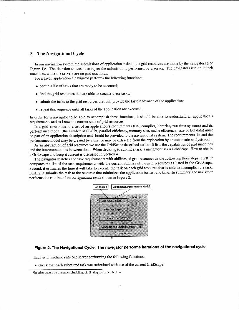
The MT can be in “monitor” mode, “probe” mode or both. In the “monitor” mode it runs NGB across all grid machines with intervals of time which are automatically adjusted accordingly to the grid volatility. (As the grid volatility we use the gradient of the benchmarks turnaround time.) The benchmarking results, including the execution time of the tasks and the communication times between machines, are recorded in the Gridscape. A visualization of the Gridscape obtained by monitoring the grid with NGB is shown in Figure 4.

Figure 4. A visualization of the Gridscape obtained with the NGB.

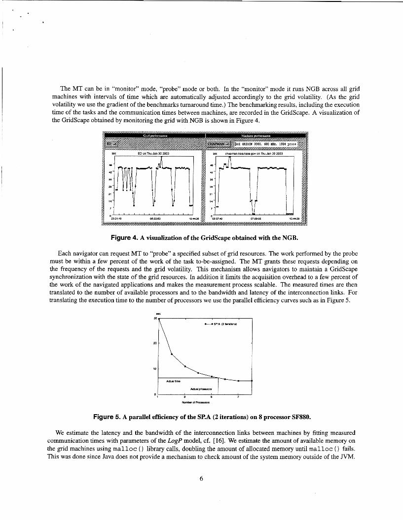
Each navigator can request MT to “probe” a specified subset of grid resources. The work performed by the probe must be within a few percent of the work of the task to-be-assigned. The MT grants these requests depending on the frequency of the requests and the grid volatility. This mechanism allows navigators to maintain a GridScape synchronization with the state of the grid resources. In addition it limits the acquisition overhead to a few percent of the work of the navigated applications and makes the measurement process scalable. The measured times are then translated to the number of available processors and to the bandwidth and latency of the interconnection links. For translating the execution time to the number of processors we use the parallel efficiency curves such as in Figure 5.

Figure 5. A parallel efficiency of the SP.A (2 iterations) on 8 processor SF880.

We estimate the latency and the bandwidth of the interconnection links between machines by fitting measured communication times with parameters of the LogP model, cf. [16]. We estimate the amount of available memory on the grid machines using malloc ( ) library calls, doubling the amount of allocated memory until malloc ( fails. This was done since Java does not provide a mechanism to check amount of the system memory outside of the JVM.

6

Currently we do not have a portable method to check the amount of available disk space on grid machines.

5 Grid Navigation of the Arithmetic Data Cube

With knowledge of the Gridscape and the application performance model, a navigator can choose grid resources and assign tasks by executing steps of the navigational cycle (see Figure 2). In this section we describe an implementation of these steps in an automatic navigation system.

In [9], we demonstrated that using a Gridscape acquired by probing with E D 3 and HC.S decreases the turnaround time in runs of VP. W and MB.W, which were chosen to represent computationally intensive CFD applications. In this paper we demonstrate navigation of a data intensive Arithmetic Data Cube (ADC) application. The ADC represents a typical computation of data warehousing and On-Line Analytical Processing (OLAP), decision support database systems, data mining systems and resource brokers. The main subject of these applications is a data set characterized by a number d of dimension attributes and a measure attribute. The data set consists of tuples (il, . . . , i d , c). Each dimension attribute ij assumes values in some range, say in an interval [l, mj], and c is a cost function (a measure) associated with the tuple (il, . . . , Z<i). The goal of OLAP is to assist users in discovering patterns and anomalies in the data set by providing short query execution times [ 191.

A standard tool of OLAP is the Data Cube Operator (DCO) [6], which computes views of the data set. For a subset of k attributes, a view is an ordered set of k-tuples containing only the attributes in the subset. If multiple d-tuples are mapped to the same k-tuple, then the measures of the d-tuples are accumulated. If technically possible, DCO computes 2d views (on all possible subsets of the dimensions).

The advantage of using a grid for computing the DCO is that the calculations may be significantly accelerated if the problem can be broken into tasks that can be performed in-core. Each task computes a subset of views and the advantage of fitting in the main memory by the splitting the work significantly outweighs the loss of reusing the data obtained in the course of computing the other views. We will demonstrate the capability of our navigation system to perform such allocation in the final version of the paper. Currently we show that even if all tasks can be computed in-core then balancing the load, which takes into account the dynamic Gridscape, improves the ADC performance.

An ADC instance is specified by a few parameters per ADC dimension. These parameters define the pseudo- random numbers used to generate the data set [lo]. For our experiments the parameters are chosen in such a way that we can a priori calculate the sizes of the views. It is commonly accepted [I41 that the DCO computation time is proportional to the view sizes. These two properties give us methods to build the ADC performance model and to provide the scheduler with data to choose the load to be assigned to each task.

For the experiments we used an implementation of ADC called AdcView3. The input of AdcView is an Arithmetic Data Set [IO]. Each row of this data set contains d dimensional attributes and m measures. All dimension attribute values and measure attribute values are integers. The AdcView output for a specified k-element subset of 2d group-by aggregations is a sorted list of k-tuples.

First, the AdcView reads data row-by-row from disk into main memory. Then, it computes a view in main memory via balanced binary trees. The dimension attributes form a tuple which is used as a key. If duplicate keys occur during an insertion then the insertion algorithm performs aggregation of corresponding measure values. So, the tree contains only unique tuples as keys and corresponding aggregated measure values. The computation of a view requires a single pass of input data. The insertions continue until all input data are read. Finally the algorithm traverses the balanced search tree and writes data to disk as a sorted view.

To speed up the data cube computation, AdcView uses well known optimization strategy [ 141 that computes a view from a smallest parent. We keep all information on already calculated (ready) views to provide an efficient search of the smallest parent.

For the experiments in this paper we chose a 9-attribute data set of of lo6 tuples and 63 views of this data set. This results in a 44MB data set and a 955MB output file containing all views of the data set; it takes about 291 sec on the

3The AdcView was provided by CrossZ Solutions.

7

fastest machine of the grid to perform the whole computation.

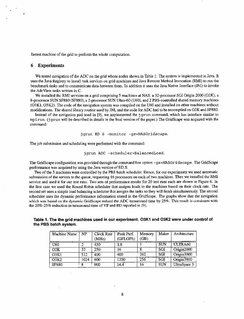
Machine Name NP Clock Rate Peak Perf. Memory

U60 2 450 1.8 1 02K 32 250 16 8 03K1 512 400 400 262 03K2 1024 600 1200 256 SF880 8 900 14.4 16

( M W (GFLOPS) (GB)

6 Experiments

Maker Architecture

SUN ULTRA60 SGI Origin2000 SGI Origin3000 SGI Origin3800 SUN UltraSparc3

We tested navigation of the ADC on the grid whose nodes shown in Table 1. The system is implemented in Java. It uses the Java Registry to install task services on grid machines and Java Remote Method Invocation ( M I ) to run the benchmark tasks and to communicate data between them. In addition it uses the Java Native Interface (JNI) to invoke the AdcView tasks written in C.

We installed the RMI services on a grid comprising 5 machines at NAS: a 32-processor SGI Origin 2000 (02K), a 8-processor SUN SF880 (SF880), a 2-processor SUN Ultra-60 (U60), and 2 PBS-controlled shared memory machines (03K1,03K2). The code of the navigation system was compiled on the U60 and installed on other machines without modifications. The shared library routine used by JNI, and the code for ADC had to be recompiled on 02K and SF880.

Instead of the navigation pad used in [9], we implemented the j grun command, which has interface similar to mpirun. ( j grun will be described in details in the final version of the paper.) The Gridscape was acquired with the command:

jgrun ED S -monitor -gs=NASGridscape.

The job submission and scheduling were performed with the command:

jgrun ADC -scheduler=BalancedLoad.

The Gridscape configuration was provided through the command line option -gs=NASGridscape. The GridScape performance was acquired by using the Java version of ED.S.

n o of the 5 machines were controlled by the PBS batch scheduler. Hence, for our experiments we used automatic submission of the servers to the queue, requesting 16 processors on each of two machines. Then we installed the M I service and used it for our test runs. Two sets of performance results for 20 test runs each are shown in Figure 6. In the first case we used the Round Robin scheduler that assigns loads to the machines based on their clock rate. The second set uses a simple load balancing scheduler that assigns the tasks so they will finish simultaneously. The second scheduler uses the dynamic performance information stored in the Gridscape. The graphs show that the navigation which was based on the dynamic Gridscape reducd the ADC turnaround time by 25%. This result is consistent with the 20%-25% reduction in turnaround time of VP and ED reported in [9].

8

see

140 -

t 1 60 I

1 6 11 16

Experiment Number

Figure 6. Navigation of AdcView with 9 attributes, lo6 tuples, and 63 views (written in C). As a scheduling algorithm we used a load balancing that has objective function of finishing all tasks on all grid machines at the same time. Here GS stands for Gridscape.

7 Conclusions and Future Work

We have described an architecture and implementation of a system that automates application navigation on com- putational grids. Our navigation system automatically acquires a map of the grid and assigns tasks of a grid application to grid machines. The system chooses resources that provide the fastest advance of application tasks and, as a result, decreases application turnaround time by 25% in our experiments. The scalability of the system is achieved by limit- ing the navigation overhead to a few percent of the application resource requirements. The navigation system follows the ‘‘WARE” protocol which guarantees that navigation does not cause congestion on the grid in the case when many applications compete for grid resources.

Mapping of the grid and scheduling of grid applications is an active research area. Some relevant dynamic schedul- ing and monitoring tools (AppLeS [2], Globus Heart Beat Monitor[l3], SCIRun [15]), and grid Metascheduler [20] use different techniques for task assignment. We are planning to enhance the capabilities of our navigation system by interfacing it with some of these tools and some measurement tools such as the Network Weather Service [21]. We are also planning to use our system to navigate real applications, in particular parameter studies, data intensive applications, and multidisciplinary applications.

Acknowledgments. We appreciate discussions of grid scheduling issues with Piyush Mehrotra.

References

[I] A. Al-Theneyan, P. Mehrotra, M. Zubair. “A Resource Brokering Infrastructure for Computational Grids.” HIPC 2002, LNCS 2552, pp. 463-473,2002.

[2] E Berman, R. Wolski, S. Figueira, J. Schopf, S. Shao. “Application Level Scheduling on Distributed Heteroge- neous Networks.” In Proceedings of Supercomputing 1996, 1996.

[3] F. Berman. “High-Performance Schedulers.” In: [8].

9

[4] G.E. Blelloch, P.B. Gibbons, Y. Matias. “Provably Efficient Scheduling for Languages with Fine-Grained Paral- lelism.” Journal ofACM, 46, (2), March 1999, pp 281-321.

[5] Grid Application Development Software (GrADS) Project. http://www.hipersoft.rice.edu/grads.

[6] J. Gray, A. Bosworth, A. Layman, and H. Prahesh. Data Cube: A Relational Aggregation Operator Generalizing Group-By, Cross-Tab, and Sub-Total. Microsoft Technical Report, MSR-TR-95-22, 1995.

[7] K. Czajkowski, S. Fitzgerald, I. Foster, C. Kesselman. “Grid Information Services for Distributed Resource Sharing.” Proceedings of HPDC-10, 7-9 August, 2001, San-Francisco, CA, pp. 181-194.

[ 8 ] The Grid. Blueprint for a New Computing Infrastructure. I. Foster, C. Kesselman, Eds., Morgan Kaufmann Publishers Inc., San Francisco, CA, 1999.

[9] M. Frumkin, R. Hood. “Navigation in Grid Space with the NAS Grid Benchmarks” Proceedings of the 14th IASTED International Conference ”Parallel and Distributed Computing and System” (PDCS’2002), Cam- bridge, USA, Nov 4-6,2002, pp.24-3 1.

Technical Report NAS-03-000. [lo] M. Frumkin, L. Shabanov. ”Arithmetic Data Cube as a Data Intensive Benchmark” To be published as NAS

[ 1 I] M. Frumkin, Rob E Van der Wijngaart. “NAS Grid Benchmarks: A Tool for Grid Space Exploration.” Proceed- ings of HPDC-10, 7-9 August, 2001, San-Francisco, CA, pp. 315-322.

[12] D. Gannon at al. “Programming the Grid: Distributed Software Components, P2P and Grid Web services for Scientific Applications.” http://www.extreme.indiana.edu/ gannon.

[ 131 “Globus Heartbeat Monitor.” http://www.-globus.org/hbm.

[14] V. Harinarayan, A. Rajaraman, and J. D. Ullman. Implementing Data Cubes Eficiently. In Proc. of ACM SIG- MOD, pp. 205-216, Montreal, Canada, June 1996.

[ 151 C.R. Johnson, S.G. Parker, D. Weinstein. “Large Scale Computational Science Applications using the SCIRun Problem Solving Environment.” Proceedings of SC 2000.

[ 161 T.T. Lee. “Evaluating Communication Performance Measurement Methods for Distributed Systems” Pro- ceedings of the 14th IASTED International Conference ”Parallel and Distributed Computing and Systems” (PDCS’2002), Cambridge, USA, Nov 4-6,2002, pp.45-51.

[ 171 “NASA Information Power Grid.” http://www.-nas.nasa.gov/IPG.

[ 181 Platform Computing. “Building Production Grids with Platform Computing.” http://www.platform.com/industry/whitepapers.

[I91 S. Sarawagi, R. Agrawal, and N. Megiddo. Discovery-driven Exploration of OLAP Data Cubes. In Proc. Inter- national Conf. of Extending Database Technology (EDBT’98), March 1998, 168-182.

[20] S.S. Vadyhiyar, J.J. Dongarra. “A Metascheduler for the Grid.” Proceedings of HPDC-11, 23-26 July, 2002, Edinburgh, Scotland, pp. 343-351.

[21] R. Wolski, N.T. Spring, J. Hayes. “The Network Weather Service: A Distributed Resource Performance Forecast- ing Service for Metacomputing.” J. Future Generation Computing Systems, 1999, also UCSD Technical Report Number TR-CS98-599, 1998, http://nws.npaci.edulNWS/.

10

Appendix A:NAS Grid Benchmarks

To make the paper self contained we include a short description of the NAS Grid Benchmarks (NGB). NGB, see [ 113 were designed to test grid functionality, performance of grid services, and to represent typical grid applications. NGB use a basic set of grid services such as create task and communicate. An NGB instance is specified by a data flow graph encapsulating NGB tasks (NAS Parallel Benchmark (NPB) codes) and communications between these tasks. Currently there are 4 types of NGB: Embarrassingly Distributed (ED), Helical Chain (HC), Visualization Pipeline (VP), and Mixed Bag (MB), as shown in Figure 7. Baseline NPB codes, specifically BT, SP, LU, MG, and FT were chosen as NGB tasks since NPB codes are well-studied, well-understood, portable, and widely accepted as scientific benchmark codes.

An instance of NGB comprises a collection of slightly modified NPB codes, each of which solves a problem defined on a fixed, logically Cartesian discretization mesh. Each NPB code (BT, SP, LU, MG, or FT) is specified by class (mesh size), number of iterations, source(s) of the input data, and consumer(s) of solution values see instances of NGB Data Flow Graphs (DFG), in Figure 7. Each DFG is constructed in such a way that there is a directed path from the source node (indicated by Launch in Figure 7 ) to any other node and from any node to the sink node of the graph (indicated by Report).

Embarrassingly Distributed (ED) Helical Chain (HC) Visualization Pipeline (VP) Mixed Bag (MB)

I ,

Figure 7. Data flow graphs of NGB, class S. Solid arrows signify data and control flow. Dashed arrows signify control flow only. Subscripts of MB tasks indicate the number of iterations carried out by an NPB code.

11