Using Gramian Theory for Actuator and Sensor Placement

Supewisov: M.C.E. Schtieiders

Content

ABSTRACT ................................................................................................................. 3

PNTRODUCTI[ON ....................................................................................................... 4

INTRODUCTION ...................................................................................................... 4

CHAPTER 1: GRAMIANS ........................................................................................ 5

.................................................................................................. 5 i . 1 INTRODUCTION 5 ............................................................................................................. 5 1.2 SYSTEM 5

............................................................................ 5 1.3 CONTROLLABILITY GRAMIAN 7 .............................................................. 5 1.4 CRITERION FOR ACTUATOR LOCATION 8

............................................................................... 5 1 . 5 OBSERVABILITY GRAMVW 9 ............................................................................. 5 1 . 6 NUMERICAL SIMPLIFICATION 9

CHAPTER 2: APPLYING GRAMIANS ................................................................ 11

................................................................................................ 5 2.1 INTRODUCTION 11 5 2.2 TEST SYSTEM .............................................................................................. 11

CHAPTER 3: BERNOUILLI-EULER BEAM ................................................... 1 6

CHAPTER 4 GRAMIAN VALIDITY ................................................................ 2 5

5 4.1 INTRODUCTION ........................................................................................... 25 ..................................... 5 4.2 VIBRATION CONTROL VERSUS MOTION CONTROL ... 2 5

5 4.3 CREATING CONTROLLER ............................................................................... 25 5 4.4 MOTION CONTROL .......................................................................................... 27

...................................................................................... 5 4.5 VIBRATION CONTROL 28 tj 4.6 VALIDATION VIBRATION CONTROL ................................................................ 2 9

CONCLUSION ............................................................................................... 3 0

SOURCES ........................................................................................................ 3 1

APPENDIX A: PROOF GRAMIAN APPROACH ............................................. 3 2

APPENDIX B: EULER-BERNOULLI ELEMENT ..................................... ... 3 3

APPENDIX C: ACTUATOR DATA SHEET ......................................................... 35

.................................................... APPENDIX D: MODAL COORDINATES 3 6

APPENDIX E: TRACKING BEHAVIOR .................................................... 3 7

APPENDIX F: IMPULSE RESPONSE .................................................................. 39

Abstract

Different placement of actuators in mechanical systems results in different system behavior. In this discussion the placement of the actuators is optimized in order suppress resonant vibrations as good as possible. Vibrations in actual experimental facilities are common and have to be avoided. There is a method that helps avoiding this, which involves the use of the controllability- and observability gramians and this will be applied.

The theory b e h d tkis apprmch wi!! be exp!zined, fe!!ewed by ~pp!ir,atien on a test system. This proved encourslging resdts and therefore this method was applied a more sophsticated system, subject to this discussion. For this system some extra influences were examined as well. In conclusion this approach for vibration control will be tested and validated.

Introduction

This traineeship is part of a much larger project and is subject of this discussion. The larger project entails control of a beam, with movable actuators and sensors. The beam itself is supported, the main goal is to try and suppress the beams resonant behavior. In mechanical systems usually actuator and sensor locations are kept at a fixed position and are known beforehand. The idea in this discussion is to optimize these positions with respect to the dynamical behavior of the system.

A method to optimize actuator sensor locations in niotion md vibrztioii control of flexible structures is based on the use of the controllability- and observability gramians. These gramians represent a quantitative measure of controllability and observability. For linear flexible systems it will be shown that this is not computationally intensive; only the eigenvalues of the gramians are needed and calculating these can be done very efficient for only the systems modal behavior is needed. In applying this method one is looking at the mechanics of the system, not needing any knowledge of the used controller. First the gramian theory will be explained in greater detail. Then this will be applied on a mass-train system via simulation to confirm and understand the method. This will be applied on a model of the beam system, used in the larger project. Here extra influences will be examined as well.

The goal of this discussion is to examine if this type of knowledge of system behavior depending on actuator and sensor placement can be used to improve system performance. The performance criteria will be defined later. Finally some conclusions and recommendations will be given.

Chapter 1 : Gramians

tj 1.1 Introduction

In flexible systems eigenmodes are inherently present. When placing an actuator in the vicinity of a nodal point of an eigenmode, the actuator will need unrealistic large forces to control this mode. Placing a sensor here would not yield useful information. The importance lies in the fact that when a system is already under a control law, this law will he unahle to control this mode! It is therefore useful to take into account the systems modal behavior. The complete system response is usually determined by a few of the lower modes. Using a method based upon the gramians it is possible to choose how many and which specific eigenmodes are included for the actuator and sensor placement optimization.

In reference [I] it is reported that only the lower eigenmodes have to be considered since higher modes (in a physical system) are harder to excite. The bandwidths of sensors and actuators cannot respond to the highest fiequent modes and also the computer capacity is limited. The gramian theory, the basis for this discussion, will be explained here.

@ 1.2 System

A lumped mass-spring-damper system is described as follows

where state vector q is (n, 1). M, B, and K are respectively the mass-, damping- and stiffness matrix all having size (n,n). The vector q can be seen as a superposition of all eigenmodes as represented by below as a result of the expansion theory

In this Equation di is the eigenfunction matrix and is the solution of the eigenvalue problem consisting of the differential Equation (1.1) without the damping term as seen in the following Equation

This can be used in writing the system into normal form. For small damping this form is allowed. This assumption is made through this entire discussion and later on some additional reasons will be stated for why damping should be small. For writing this system into normal form, Equation (1.2) is substituted in Equation (1.1) yielding the following

q(t) = @q(t);q(t) = @?j(t);q(t) = @ ij(t)

M@ij(t) + Bp@7j(t) + K@q(t) = f ( t ) (1.4)

Pre multiplied by @T standardization occurs to the system matrices, which results in the normal form presented below

@'M@ ij(t) + @'~,@7j(t) + @'K@ q(t) = @'f ( t )

By normalizing to the mass matrix, the modal mass matrix becomes a unity matrix: @'M@ = M , = I. The damping and stifhess matrix both become diagonal matrices.

The system can be written as is seen below

This can be done only if C, is chosen diagonally with 2401, on the diagonal. The term 6 [-I denotes the choice for modal damping. All equations of motion are now decoupled and are similar to a set of independent 2" order equations.

Figure 1.1 : 2nd order mass spring system

In [2] the system is converted into state space form, with state vector q as

with fhe advantage that modal displacement and modal velocity corresponding to each mode are now about the same magnitude. This has computational advantages and is therefore implemented. This yields a state space representation as stated below, written for single input single output system at positionp

where the system matrices are defined as follows

Suffixp in Equations (1.9a) and (1.9b) denote the actuator position. Currently matrix C represents position sensors. If velocity sensors are used the matrix has to be altered slightly.

@ 1.3 Controllability Gramian

An actuator in a structure should be placed in such a way that the structure can be controlled with minimum effort and disturbances can be controlled optimally. This minimum effort can be calculated by solving the following minimum energy problem [31

T T Minimize T(u) = I, u (t)u(t)dt , (1.10)

as known as the optimal control problem to change the system from x(0)=xo to x(T)=xT. Here T denotes a terminal time or end time. With this terminal time a terminal constraint is given, which yields that this problem is numerically solvable ([3]). The terminal time is related to the systems response (e.g. speed of response) and is usually unknown this early stage in the design process. Equation (1.10) can be expanded to take into account boundary values of systems input and state during transition. These conditions will effect this terminal time ([3]).

For a system is positioned towards a desired state as a result of an input u(4. The optimal solution for this problem is given by the following Equations as seen in P I and P I

Equation (1.1 1) for minimum control energy (T- ) contains the term wl(T). W represents the controllability gramian and is defined as follows [2] and [4]

Since the reciprocal of the gramian appears in the minimal control energy it means that if w'(T) is small, some states can be positioned from xo to XT only if very large inputs are used. If W'(V is small it means its eigenvalues are small because of de decoupled nature of this system. Also this is almost the same as stating its diagonal elements are small, since it is (almost) a diagonal matrix provided modal damping ratio (6) is low. An extra condition is that the eigenvalues have to be well spaced. This

is explained in more detail in 121. When these assumptions hold the energy transfer to specific modes is high for larger values of the eigenvalues of the gramians then for low values.

In Appendix A it is proven that Equation (1.13) holds for T -+ oo, given that the system matrix A is asymptotically stable

We denotes a steady state solution as seen in Appendix A. This is a Lyapunov equation of which the result is the time independent controllability gramian W' for t -+ co. It is proven, [2], that when taking the terminal time T -+ oo the term W(T) will equal this constant We. The choice of T influences the modes and by taking an infinite terminal time this dependency is eliminated. This has a number of advantages as mentioned in [2]. However choosing an infinite terminal time has a huge consequence on the optimal input seen in Equation (1.1 1).

The link between the controllability gramian and the system is of importance for it will result in an optimal location for actuators. From [2] it follows that the system energy (kinetic and potential) can be written as a sum of energetic contributions from each mode

Both expressions in Equation (1.14) can be expanded as seen in [2]. It can be proven that the eigenvalues of the controllability gramians are equal to these expanded expressions added together to form the total energy of the system (kinetic and potential energy). This is true if damping ratio is small and the eigenfrequencies are well spaced. It means the assumptions taken still guarantee the gramians reflect systems energy.

5 1.4 Criterion for Actuator Location

A criterion is needed to easily see if an actuator is ill placed on a specific location or not. This performance index should drop sharply around the nodal points of a mode. If the first few eigenmodes are taken into account in actuator/sensor placement, more of these drops will occur. In [2] a performance index is suggested, which is in fact

- - -

energy based. This performance index is presented here f 2 n \ Izn

Here A represent the eigenvalues of the controllability matrix. If an eigenvalue tends to zero, it means an actuator is close to a nodal point and the PI should drop sharply. An advantage of this index is the use of the product. If only one gramian eigenvalue (representing an eigenmode) is small the PI will drop as it should.

-

fj 1.5 Observability Gramian

For the sensor location the solution for optimizing position is very similar to that of the actuator. Observability can be seen as the quality a mode can be measured from the system. This means the contribution of individual modes should be high to warrant high observability in a specific position. If the system is released from x(0) =xo with u(t) =O and t _> O output energy is defined in the following Equation

where Q is the obsewability gramian [2], which is shown in the following Equation.

This gramian is also nearly diagonal, which means the observability gramian is nearly singular (one or more eigenvalue(s) nearly zero) some initial inputs have little effect on the output. Again the solution (appendix A) for time to infinity

holds given the fact that system matrix A is asymptotically stable. Similar as for the controllability matrix the eigenvalues represent the observability. Because of the similarity only the performance index is given. The A seen in Equation (1.15) now represents the eigenvalue of the observability gramian.

fj 1.6 Numerical simplification

There is a way of computing the eigenvalues of the gramians directly from the modal properties of the system. It is stated that modal damping must be low for Equation (1 -3) to hold. The gramians have terms on the diagonal values, which are proportional to l/C. All other terms of the matrix are either independent or proportional to r meaning that for a low modal damping the gramians turn into diagonal matrices. Eigenvalues are the diagonal element of diagonal matrices. Therefore we can simplify the gramians

( 'd i i 'd i i 1 Qii = diag ----- -- 4riwi 4riwi

This means that the eigenvalues needed for the performance indexes (Equation (1.15)) can be directly calculated for any actuator and sensor location. The information

needed are the modal parameters: eigenvalues, eigenhnctions and damping coefficients. This provides with a simpler numerical way for calculating the performance indexes.

Chapter 2: Applying Gramians

t j 2.1 Introduction

Chapter 1 explained the theory idea behind the gramians. Before applying the gramians to the more complicated beam structure, first a simpler system is used. This is done to get a feeling in using the gramians.

8 2.2 Test System

A mass train system is used. The mass train is depicted in Figure 2.1.

Figure 2.1: Mass train (4 masses depicted)

The system is fixed to the existing world with a weak spring and damper. This damper spring combination is needed to guarantee the modal form is indeed decoupled. Without this first damper connecting the mass train to the fixed wall QT&@ will not be diagonal.

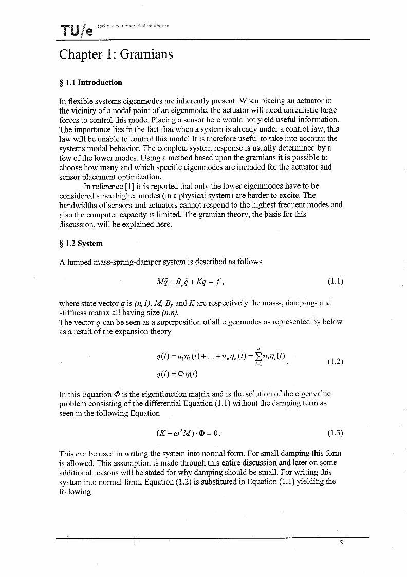
This system is written in the state space formulation as stated in Equation (1.7). The specific second order differential equation for this system stated in Equation (1. l), will be written in normal form as mentioned earlier. First only one actuator and sensor are applied. The first nine eigenmodes of this system are depicted in Figure 2.2.

e.f.:0.64244 [Hz] '- e.f.3 1.7381 [Hz]

ef . 46 499 [Hz]

-0 5

$0 20 30

10 20 30

e.f.:57.8804 [Hz]

10 20 30

Figure 2.2: First nine eigenmodes; ylabel: scaled displacement eigenmode, xlabel: beam elements. The first eigenmode (rigid body mode) can be seen in top left of Figure 2.2. The gramian theory is applied for the first and second mode (Figures 2.3 and 2.4).

, .go5 PI C G., n o.e =30 3 65

3 6

- A 8 3 55 !i

3.5

Elements Elements

ergen mode

5 10 15 20 25 30 Elements

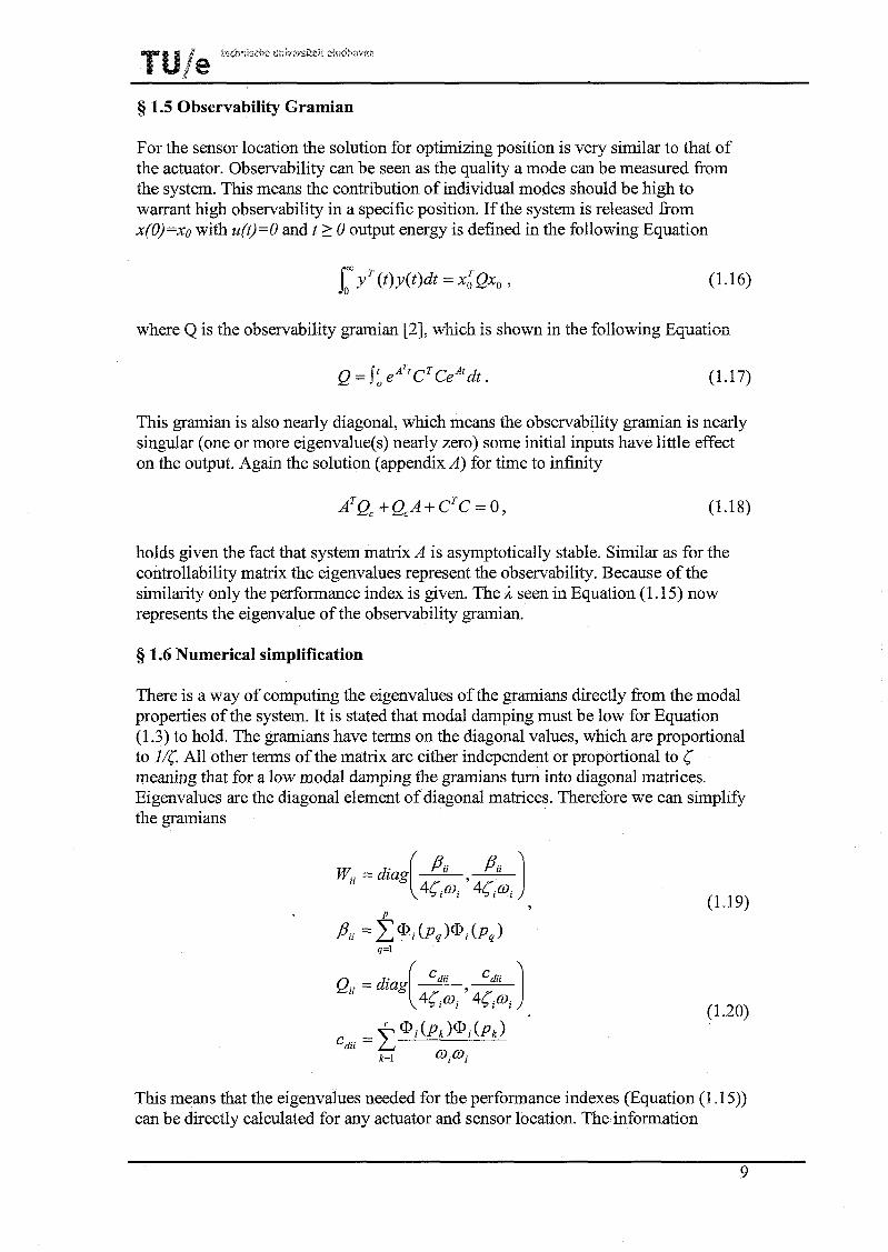
Figure 2.3: First eigenmode gramian result; C.G is Controllability Gramian, O.G. is Observability Gramian

PI O.G.. n.0.e. =30 ,106 PI C.G., n.0.e. =30 6 I

EIements

scaled Pls

Elements

Elernents

eigen mode

Elements

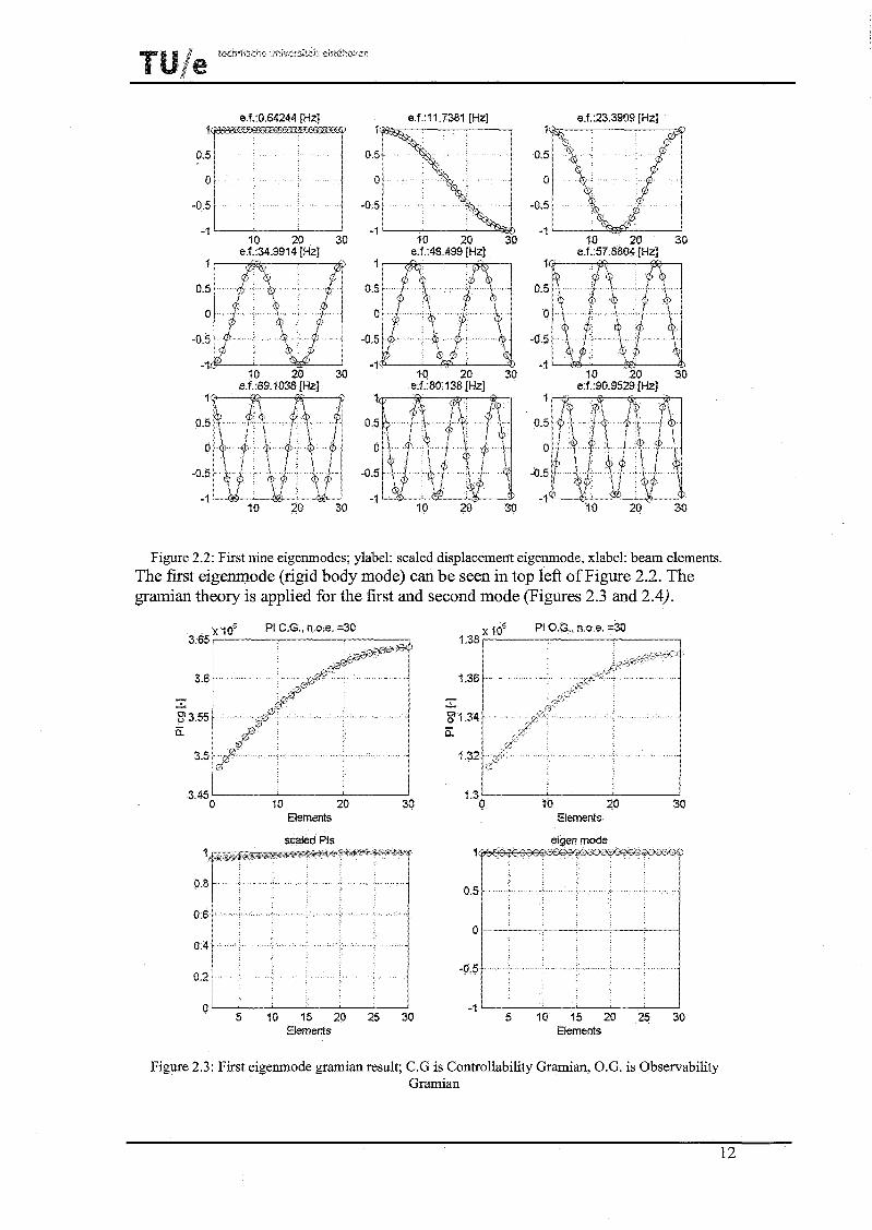
Figure 2.4: Second eigenmode gramian result, the second eigenmode is depicted in the right bottom figure; n.0.e is number of elements.

In these performance indexes only the eigenmode represented in the lower right plot of the figure was considered. The diagonal elements were used here instead of the eigenvalues of the gramian matrices. When taking the eigenvalues, using the eigenvectors is needed for coupling these values to the original states. This is numerically easier, and provides the same results theoretically. It has been verified and for small damping both methods are equal. However coupling the eigenvalues to the corresponding states proves difficulty. This will be explained in detail in Section 6.3.

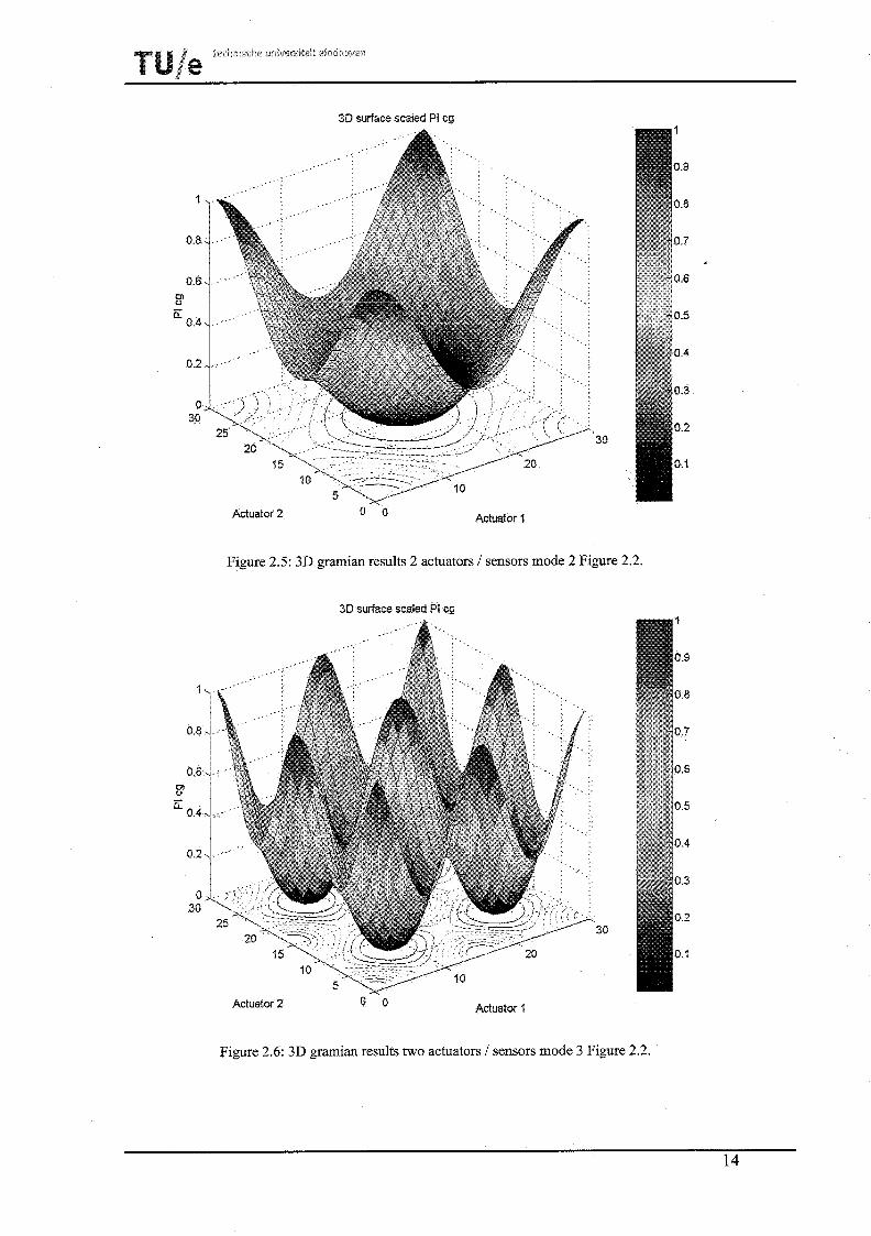
Before interpreting Figures 2.3 and 2.4 first what should be expected is mentioned. The first mode (Figure 2.3) is a rigid body mode. This eigenmode has no nodal point and therefore all positions of the beam should result into the same value for the performance index of controllability as well as observability. The results show this, the scaled performance indexes give the best representation. The rigid body mode is not completely rigid; this is seen in the eigenmode (Figure 2.2) and in the performance indexes. This is due to the small spring-damper that connects the mass train to the existing world. The second mode has a nodal point in the center. As explained in Chapter 1, the performance index should be zero at this point. From just off the middle position till the start (or end) of the masstrain the eigenmode starts to increase in absolute value (represented scaled) and so should the performance indicis. As seen in Figure 2.4 this is correct and shown. For higher order eigenmodes the results also confirm the theory. For two actuators and two sensors a three dimensional representation can be given of the gramian results with on the two axis the first and second actuator 1 sensor location and the performance index on the remaining axis. Figure 2.5 and 2.6 are the representations of the second and third mode seen in Figure 2.2.

3 0 surface scaled PI cg

Actuator 2 5 5 Actuator 'I

Figure 2.5: 3D gramim results 2 actuators / sensors mode 2 Figure 2.2.

3 0 surface scaled PI cg

Actuator 2 0 '5 Actuator I

Figure 2.6: 3D gramian results two actuators / sensors mode 3 Figure 2.2.

These two 3D representations in scaled form equal the results obtained in the case of one actuator / sensor if only the two diagonal positions are viewed (a crosscut of Figure 2.5 and 2.6). As seen the results again confirm what is theoretically expected. On the nodal points the performance indexes equal zero, around the nodal points the performance index slightly increases. On points of great excitation the performance index goes towards a scaled value of 1. As can be seen in Figures 2.2,2.5 and 2.6 the number of nodal points in the eigenmode is the same as the number of dips on the diagonal of Figures 2.5 and 2.6. Also the scaled performance indexes of the observability and controllability are equal.

Chapter 3 : Bernouilli-Euler Beam

5 3.1 Introduction

In this Chapter gramian theory is applied to a model of a beam structure. The beam system will first be defined, and then the gramian theory will be applied. The chosen position of actuator / sensor will have consequences for the system with respect to mass for instance. This will also be extended on here.

5 3.2 Beam system

The beam system is represented in the Figure 3.1 and consists of Bernoulli-Euler elements.

Wl01 w292 w3 93 w4 94 w5 95

Figure 3.1: Beam system; 4 elements, 10 degrees of fieedom depicted

In [5] this type of element is mentioned with explanation about its make up. The resulting element matrices are stated in as follows

where p = material density [kg/m3]; A = element cross-section [m2]; 1 = element length [m]; E = Material Young's Moddus [Pa]; I = element second moment of inertia [m4].

The damping matrix is chosen to be a factor 1 o - ~ times the stifhess matrix. The mathematical background that defines this type of element is given in Appendix B, which is based upon [5], [6] and [7]. The coordinate vector for this system is stated in Equation (3.2) with suffix n the number of elements

tj 3.3 Gramians Applied

Applying these gramians to this beam system is very similar to the application on the mass train system discussed earlier. The eigenmodes are depicted in Figure 3.2.

e.f.:0.1802 [Hz] 1

i -0.5 -1 I 10 20 30

ef.: 117.6194rHzl

I0 20 30 e.f.:569.4290 [Hz]

-0.5

$0 20 30

e.f.:0.3132 [Hz]

10 20 30 e.f.. 230.5824 [Hz]

I-

e.f.:42.6705 [Hz]

I 0 20 30 e.f. 381.1723 [Hz]

0 I

w -1

10 20 30 e f.: 1.0590e+003 [Hz]

-1- 10 20 30

Figure 3.2: Beam system first nine eigenmodes presented in translation form. Rotational form si excluded

The results for the third eigenmode (the first two are rigid body modes) are presented below.

PI C.G.. n.0.e. = 30

D.O.F.

$0-7 Pt O.G., n.0.e. = 30

"7

Figure 3.3: Beam system Performance Indexes only the third eigenmode considered; 1 actuator and 1 sensor.

The eigenmodes in Figure 3.3 are represented in a translational and rotational way and individually plotted. The performance indexes again confirm what is expected based upon the eigenmode.

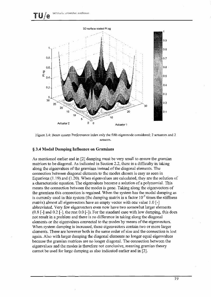
Applying the gramian theory upon the beam a three dimensional representation of the indexes with two actuators and two sensors is presented. This is done for the fourth eigenmode containing three nodal points. These can be found in Figure 3.4.

3D surface scaled PI cg

Actuator 2 Actuator 1

Figure 3.4: Beam system Performance index only the fifth eigenmode considered; 2 actuators and 2 sensors.

$j 3.4 Modal Damping Influence on Grarnians

As mentioned earlier and in [2] damping must be very small to ensure the gramian matrices to be diagonal. As indicated in Section 2.2, there is a difficulty in taking along the eigenvalues of the gramians instead of the diagonal elements. The connection between diagonal elements to the modes chosen is easy as seen in Equations (1.19) and (1.20). When eigenvalues are calculated, they are the solution of a characteristic equation. The eigenvalues become a solution of a polynomial. This means the connection between the modes is gone. Taking along the eigenvectors of the gramians this connection is regained. When the system has the modal damping as is currently used in this systea (the damping matrix is a factor times the stiffness matrix) almost all eigenvectors have an empty vector with one value 1.0 [-I abbreviated. Very few eigenvectors even now have two somewhat larger elements (0.8 [-I and 0.2 [-I, the rest 0.0 [-I). For the standard case with Pow damping, this does not result in a problem and there is no difference in taking along the diagonal elements or the eigenvalues connected to the modes by means of the eigenvectors. When system damping is increased, these eigenvectors contain two or more larger elements. These are however both in the same order of size and the connection is lost again. Also with larger damping the diagonal elements no longer equal eigenvalues because the gramian matrices are no longer diagonal. The connection between the eigenvalues and the modes is therefore not conclusive, meaning gramian theory cannot be used for large damping as also indicated earlier and in [2].

t j 3.5 Mass influence actuator on Grarnians

The data sheet of the actuator is given in Appendix C. It is a coil, which can be used to apply force as a result of current applied on it. It is interesting to see the influence the mass has. The effect on the gramians will be examined and an explanation is sought.

Mass can be added numerically in several ways. For instance one can add a point mass on the exact node on which the actuator is placed or increase the mass of elements left and right of the node the actuator is placed. Both give about the same result as will be shown. There is a difference in absolute mass addition sense in the two approaches because it is hard to exactly q u a i point mass and eiement mass. Tne shapes are the same and represented in Figure 3.5. Further mass is added aiong the beam for one actuator only.

Figure 3.5: Performance iodexes with mass influence, higher graphical line consists with higher mass in the top two plots of the figure.

The results show two important aspects for this first mode (this mode is chosen to easily see the influences). The controllability performance index shows a higher value at the ends for a higher mass and the value is the same for the middle position. This result should reflect what is seen in the eigenmodes presented in Figure 3.6.

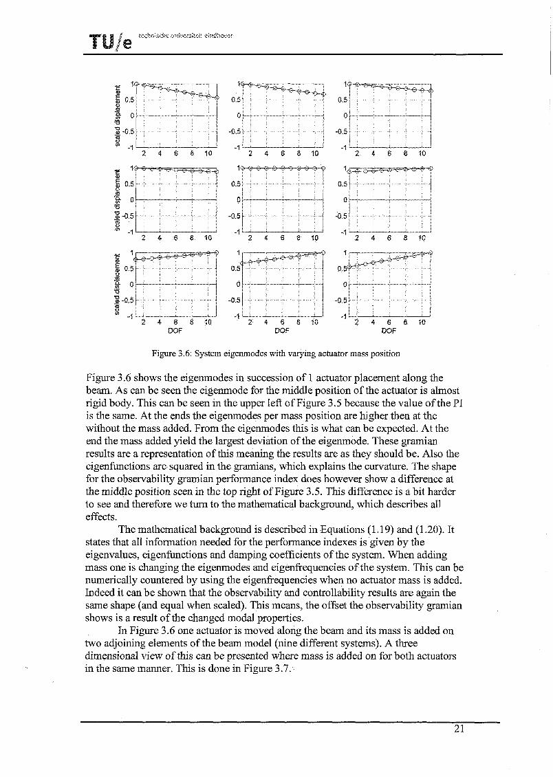
Figure 3.6: System eigenmodes with varying actuator mass position

Figure 3.6 shows the eigenmodes in succession of 1 actuator placement along the beam. As can be seen the eigenmode for the middle position of the actuator is almost rigid body. This can be seen in the upper left of Figure 3.5 because the value of the PI is the same. At the ends the eigenmodes per mass position are higher then at the without the mass added. From the eigenmodes this is what can be expected. At the end the mass added yield the largest deviation of the eigenrnode. These gramian results are a representation of this meaning the results are as they should be. Also the eigenfunctions are squared in the gramians, which explains the curvature. The shape for the observability gramian performance index does however show a difference at the middle position seen in the top right of Figure 3.5. This difference is a bit harder to see and therefore we turn to the mathematical background, which describes all effects.

The mathematical background is described in Equations (1.19) and (1 -20). It states that all information needed for the performance indexes is given by the eigenvalues, eigenfunctions and damping coefficients of the system. When adding mass one is changing the eigenmodes and eigenfi-equencies of the system. This can be numerically countered by using the eigenfi-equencies when no actuator mass is added. Indeed it can be shown that the observability and controllability results are again the same shape (and equal when scaled). This means, the offset the observability gramian shows is a result of the changed modal properties.

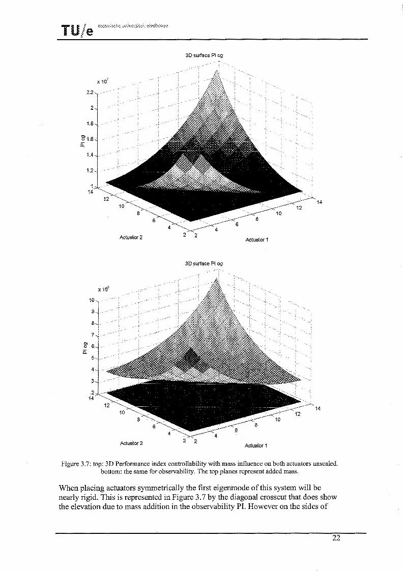
In Figure 3.6 one actuator is moved along the beam and its mass is added on two adjoining elements of the beam model (nine different systems). A three dimensional view of this can be presented where mass is added on for both actuators in the same manner. This is done in Figure 3.7.

3D surface PI cg

Actuator 2 2 2 Actuator 1

3D surface PI og

Actuator 2 Actuator t

Figure 3.7: top: 3D Performance index controllability with mass influence on both actuators unscaled. bottom: the same for observability. The top planes represent added mass.

When placing actuators symmetrically the first eigenrnode of this system will be nearly rigid. This is represented in Figure 3.7 by the diagonal crosscut that does show the elevation due to mass addition in the observability PI. However on the sides of

this cross cut the mass less situation is resembled. The other crosscut resembles the case where one mass is moved along the beam only twice as much (two actuators).

For this mode the influence is shown and an explanation is found. The same can be done for other modes and the explanation can be sought in the systems modal behavior.

5 3.6 Stiffness Influence Actuator on Gramians

The same background that has been described in the previous Section can account for the results of stiffness variation. Here the same way the mass can influence the total Seam system; now the stiffness is changed at the actuator position. The two surrounding elements to the actuator position have added stiffness modeled. For the actual system this would mean flexibility would change locally on position of actuator connection. Again a two dimensional and a three dimensional representation are given, respectively in Figure 3.8 and 3.9. Figure 3.8 presents the case for a single actuator resembling the diagonal crosscut of Figure 3.9 (the line where actuator 1 and 2 have equal position). What can be seen clearly from the scaled representation of the performance indexes in Figure 3.8 is the small difference. The three dimensional representation for the added stiffness does show a less smooth graphical representation (lower green plane). This again is a consequence of the modal behavior.

DOF

Figure 3.8: Performance indexes with stiffness influence, higher graphical line consists with higher local stiffhess.

3D surface PI cg

Actuator 2 2 - 2 Actuator I

-. Actuator 2 2 2

Actuator 1

Figure 3.9: top: 3D Performance index controllability with stiffness influence on both actuators unsealed. bottom: the same for observability. Top planes represent added stiffness.

Chapter 4 Gramian Validity

tj 4.1 Introduction

Adding a controller to the system will enable it to follow a certain trajectory. Vibration control entails that disturbances on a system must be dealt with and this is dependent of the actuatorlsensor placement. In motion control, the goal is different as will be shown. In this Chapter a controller for tracking will be derived. This will be fdowed by the app!ic&ion ef metien control a d ! ~ ~ k i ~ g 2t this from both mnh-01 and a vibration point of view. Concluding the results will be given regarding the value and usability of vibration control.

tj 4.2 Vibration control versus motion control

Experimental setups experience disturbances that can excite eigenmodes. Such disturbances can then result in a vibration that cannot be influenced by actuators. From a vibration control viewpoint these nodal positions have to be avoided. In motion control this is different. Actuating a system to track a certain path, the modal coordinates reveal the amount of error of each eigenmode. If one eigenmode is domixmt and the actmtsrs are placed at the nodal point of that particular mode, then the belonging modal coordinate will be negligibly small. This mode will not be visible in the systems behavior. Nodal points are tkis preferable in motion control. This means there are contradiction demands for vibration and motion control.

5 4.3 Creating Controller

To ensure equal bandwidth of the open loop system with different actuator placement the controller should be adjusted per position. This is because of the difference in system due to actuator placement. This is shown in the following Figure.

Figure 4.1 : Transfer functions for three beamsystems (three actuator/sensor placements); legend order is the same order as graph from top to bottom at 1 [radls]

Here three systems are shown. A beam system consisting of 21 beam elements with actuators placed as denoted in the legend of Figure 4.1 .Although different system behavior is seen the middle position is used for creation of a controller, which is used in all simulations. An easy and effective way of creating a controller for the system is by means of the Matlab routine DIET (Do It Easy Tool). The result of such a tuning can be seen in Figure 4.2'.

Freauencv R e s ~ o n e e

Frequency [Hz]

Frequency [Hz]

Figure 4.2: Tuning the system to a desired bandwidth as seen in open loop behavior

1 Only the general idea of controlling is presented. The resonance peak around 42 [Hz] can be dealt with.

For controller a simple lead lag is chosen, this provided enough for system stability. The exact controller used is seen in Equation (4.1). The frequencies are chosen logarithmically symmetric around 10 [Hz] resulting in a stabilizing phase advantage at that fi-equency

where P = 100 [-I; fl = 10/3 = 3.33 [Hz]; fi= 10*3 = 30 [Hz].

5 4.4 Motion Control

Two actuator$ will actuate the beam system symmetrically and in the same direction under the same control law. This means certain modes will not be able to be excited. The mode shapes are shown in Figure 3.2 and it is easy to understand the second mode will not be able to be excited because of the symmetric actuator. Simulations also reveal this, the second2, fourth, sixth, etc. modal parameter is, when plotted against time, negligible small. The system will follow the desired path as seen in Figure 4.3. The path is obtained f?om the larger project in which this is desired.

Figure 4.3: prescribed motion path

In Appendix D the first eight modal coordinates are presented. As can be seen the fifth modal coordinate has the same order as the third. In a system containing 23 elements the (closest thing to) nodal points of mode 3 lie at node 6 and 19. Mode 5 has its two peaks or maximums there.

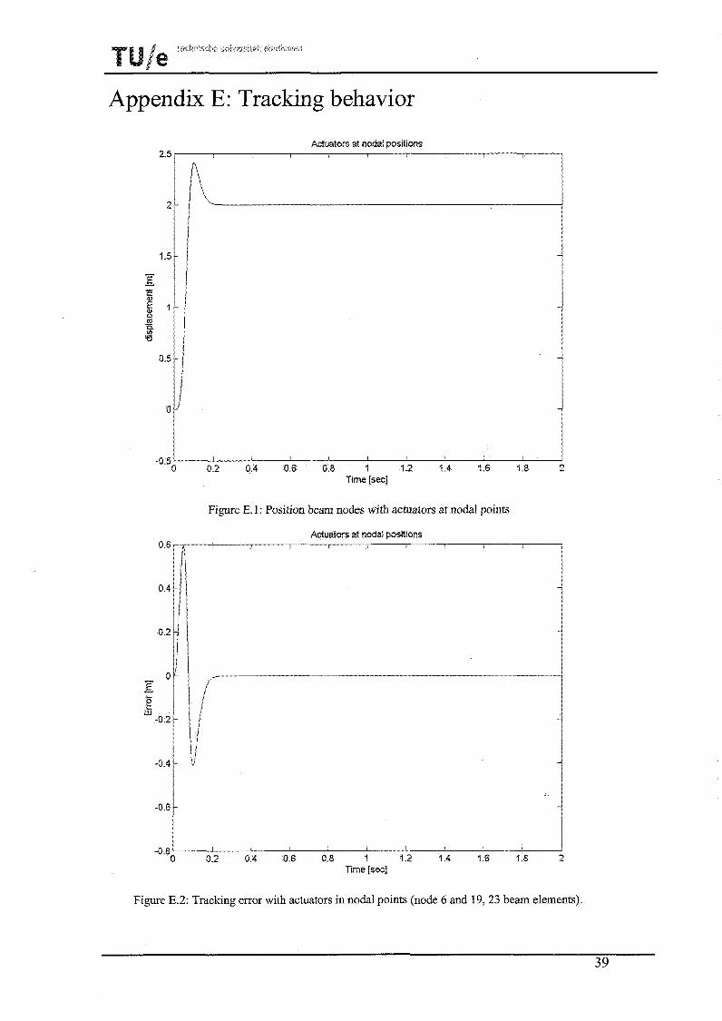
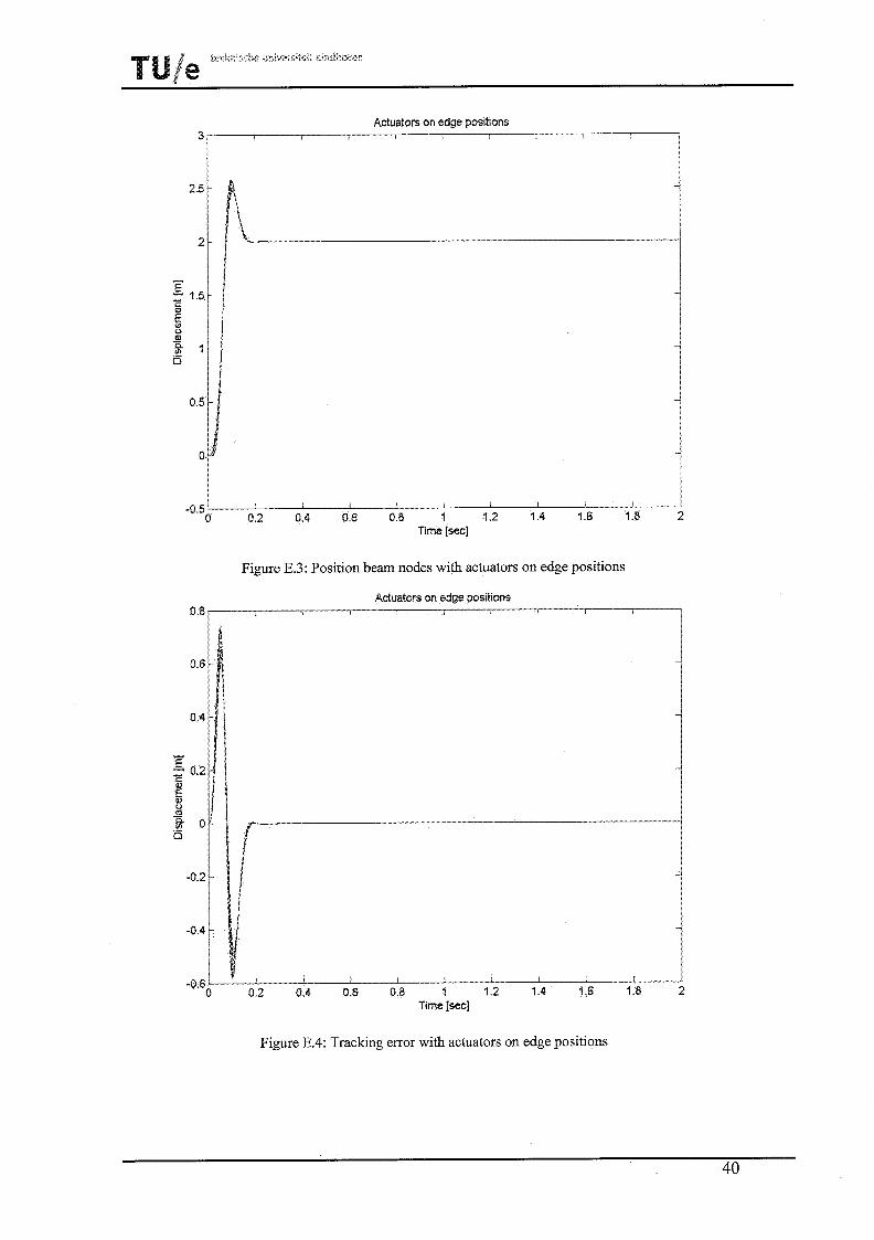
The tracking behavior when deviating actuator position is depicted in Appendix E. Two motion control situations are simulated and trzcking ccntrol is compared. The choice of the two situations will be further explained in Section 4.5. The first situation is when the actuators are placed in the nodal positions (Node 6 and 19). The second situation is moving the actuators to the edges. Comparing Figure E.2 with E.4 confirms what is to be expected based upon motion control. The error is the

q2 is of order 104but multiplied with its eigencolumn its effect negligible on physical coordinates.

27

smallest when actuators are placed in the nodal points. In addition the edge positions yield a controlled system, which when compared has a higher cross over fkequency. The systems transfer function is the top one in Figure 4.1 so it is logical that when using the same controller as in the nodal situation cross over frequency is higher. Even with this higher cross over frequency the system performs worse in the edge positions. This confirms that tracking can be done best when actuating in nodal positions.

Important to realize is that the number of elements and thus the number of points is discrete. This means that when a node is picked it can be simply very near the nodal point but not exactly on it. This can be seen in Appendix D where the third modal coordinate is not negligible but in the order of 1 * 1 W3. This discrete problem remains even when taking 100 elements. When the nodes closest to nodal positions were taken (large matrices thus large computational time) node 23 and 79 had their 'almost negligible9 eigenmode deviation in the opposite direction of the deviation in eigenmodes at those nodes at the fifth eigenmode (Figure 3.2). Node 24 and 78 had this deviation in the same direction. This can be seen in Figure 4.4. This small discrete step reversed the modal influence. Keeping the same system description it is to be accepted that the exact nodal points will not be excited. This is important when validating the gramian theory.

Figure 4.4: Visualizing the discrete problem when taking along 100 elements

, 04 Node 23 and 79 , 10-3 Mode 24 end 78

5 4.5 Vibration control

As Equation (1.2) states, the physical coordinates are summations of the modal coordinates. The modal coordinates will be seen as a 'cause' and as such can be used in the performance indexes. When applying vibration control a choice in actuator

1 5-

I - - " - o r

I , , , -5 0 0.5 1 1.5 2 -1 0 - 0.5 1 1.5 2

1 I1

V

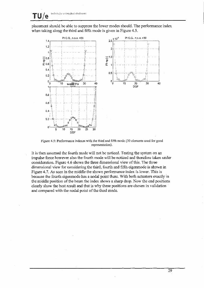
placement should be able to suppress the lower modes should. The performance index when talung along the thud and fifth mode is given in Figure 4.5.

lo-s PI O.G.. n.0.e. =30 Pt C.G., n.0.e. =30 1.4

DOF

1.2

DOF

i

Figure 4.5: Performance indexes with the third and fifth mode (30 elements used for good representation).

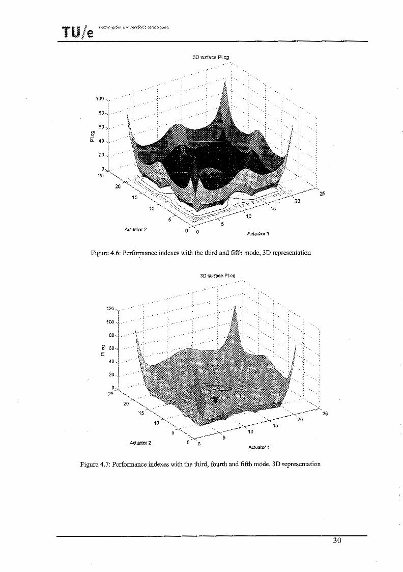
It is then assumed the fourth mode will not be noticed. Testing the system on an impulse force however also the fourth mode will be noticed and therefore taken under consideration. Figure 4.6 shows the three dimensional view of this. The three dimensional view for considering the third, fourth and fifth eigenmode is shown in Figure 4.7. As seen in the middle the shown performance index is lower. This is because the fourth eigenmode has a nodal point there. With both actuators exactly in the middle position of the beam the index shows a sharp drop. Now the end positions clearly show the best result and that is why these positions are chosen in validation and compared with the nodal point of the thrd mode.

3D surface PI cg

Actuator 2 Actuator 1

Figure 4.6: Performance indexes with the third and fifth mode, 3D representation

3D surface PI cg

Actuator 2 Actuator 1

Figure 4.7: Performance indexes with the third, fourth and fifth mode, 3D representation

5 4.6 Validation Vibration Control

Appendix F shows the results of a simulation with an 'impulse' force (of 0.01 sec and an amplitude 10 [N]) placed on the middle of the beam. The beam is then left to settle again to the original condition. The chosen two situations are with the actuators on the beams edges and in the mentioned nodal positions of the third eigenmode. Figure F. 1 shows the first four modes for both situations. The third modal coordinate is important for it shows the validity of this gramian theory. In the nodal position the influence of this mode is smaller in size, but as can be seen especially in the enlarged Figure F.2, the mode is less damped. The oscillations in this mode go on longer then in the situation where the actuators are placed on the edges. When the actuators are placed here the third mode is more easily suppressible. This concludes proving the validity of the gramian theory.

Conclusion

The theory of controllability and observability gramians is shown to have a representative view on system behavior. However a number of assumptions about the system have to hold such as well-spaced eigenfiequencies and low modal damping. These assumptions and their consequences have been confirmed and seen as valid assumptions. They even gave some numerical advantages and these advantages did not lower accuracy, which is important since it simplifies calculation. Taking along actuator mass and stiffness is pcssible and showed logical results. The concepts motion and vibration control are very different as has been shown. Both concepts have been presented and shown to work or act as expected. Since the gramains are a representation of modal information about the system they can always be taken into account when vibrations are noticed or anticipated. However an experimental modal analysis would be required in application.

The problem that remains now is where does one place emphasis; tracking behavior or vibration behavior. They cancel each other out meaning a sort of balance between the two is either case dependent or kept as variable in the control problem. When keeping it as variable one could chose to switch actuator positions when the influence of the vibration becomes too large. However ths will give rise to other problems, e.g. the time needed to switch between 2 actuator positions will have to be looked at more thoroughly.

Sources

[I]: S. Kondoh, C. Yatomi and K. Inoue. Thepositioning of sensors and actuators in the vibration control ofJlexible systems. JSME International Journal Series 3, vo1.33, No. 2, (1990)

[2]: A. Hac and L. Liu, Sensor and actuator location in motion control offlexible structures. Journal of Sound and Vibration. (1 993)

[33: A.E. Bryson and Y.C. Ho. Applied Optimal Cont~ol, Optimizcztion, Estimation and Control. New York: Hemisphere. (1 975)

[4] : A. Arbel,. Controllability measures and actuator placement in oscillatory systems, International Journal of Control 33 565-574 (1 98 1).

[5]: J.H.P.de Vree, Eindige Elementen Methode, coarse script EEM 4A680, (2000)

[6] : J. Faleskog, Finita element-metodenfir Euler-Bernoulli balk. Institutionen f i r hi%llfasthetsliira KTH, (2000)

[7]: W.A.M.Brekelmans, Platen en schalen deel I : balken en platen, coarse script Structurele Mechanics, (1 996)

[8]: B.G.Dijkstra, N.J.Rambaratsingh,C.Scherer, 0.H.Bosgra and M.Steinbuch, S. Kerssemakers. Input design for optimal discrete time point-to-point motion of an industrial XY-positioning table. Preceedings of the Conference on Decision and Control. (2000).

[9]: D. de Roover and F. B. Sperling. Point-to-point control of a high accuracy positioning mechanism. Proceedings of the American Control Conference, (1 997)

Appendix A: Proof Gramian Approach

The following basic mathematical statement is used in proving Equations (1.13) and (1.18)

In proving Equation (1.13) the following holds T ~~t w = 1; eAtBB e dt,

This results in a time dependant relation. For time going to infinity the system, if A is asymptotically stable, will settle. Thus W(t) will go towards a constant 'steady state' Wc. If W(t) goes to a constant its time derivative goes to 0

and this is the same as stated in Equation (1.13). In proving Equation (1.18) the following holds which is very similar to what is mentioned above

Again for time goes to infinity the system, if A is asymptotically stable, will settle. Then the time derivative goes to 0 as seen in the following equation

Appendix B: Euler-Bernoulli Element

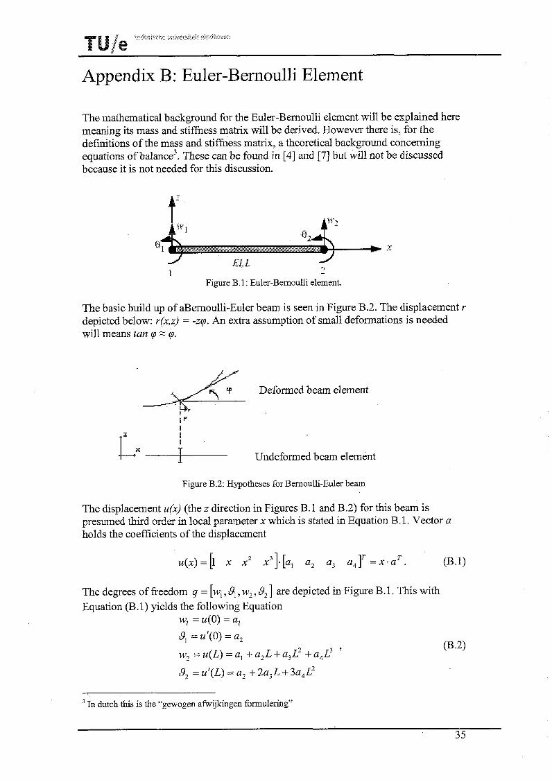
The mathematical background for the Euler-Bernoulli element will be explained here meaning its mass and stiffness matrix will be derived. However there is, for the definitions of the mass and stiffness matrix, a theoretical background concerning equations of balance3. These can be found in [4] and [7] but will not be discussed because it is not needed for this discussion.

EI. 2. - 1 -

Figure B. 1 : Euler-Bernoulli element.

The basic build up of aBernoulli-Euler beam is seen in Figure B.2. The displacement r depicted below: r(x,z) = -zq. An extra assumption of small deformations is needed will tan q - q.

Deformed beam element

1''- I I

' Undeformed beam element

Figure B.2: Hypotheses for Bernoulli-Euler beam

The displacement u(x) (the z direction in Figures B.l and B.2) for this beam is presu~fled third order in local parameter x which is stzited in Equation R. 1. Vector a holds the coefficients of the displacement

The degrees of freedom q = [w, , 9, , w, ,$,I are depicted in Figure B. 1. This with Equation (B. 1) yields the following Equation

wl = u(0) = a,

8, = ur(0) = a,

w, =u(L)=a, +a2L+a,L2 +a4L3 '

9, = ul(L) = a, + 2a3L + 3a4L2

-

In dutch this is the "gewogen afwijkingen formulering"

which can be represented as below

This means that aT = c - ' ~ , which in turn means that u(x) = xC-lq = Nq . This I - r Lraismrms the degrees of fieedom iiito a coiitiiiuoii~ &si;!aze=efit f~mi;;!ation. This is also known as the method of Galerkin, which creates a discrete displacement function. The vector N contains the interpolation functions for displacement. From [4] a definition for the mass matrix is given and is stated in the following Equation

Vector N can be derived by multiplying x and c', which yields the following Equation

Combining Equation (B.5) and Equation (B.4) then yields the element description as stated in Equation (3.1). For the stifhess matrix the special notation of the equations of balance (weighed difference method) has to be manipulated. This is described excellent in the first chapter of [7] and will therefore not be presented here. The result for the equation of the stifhess matrix is stated in the following Equation

This is Vector B is defined as the second derivative of vector N with respect to x. This yields for vector B:

Combining Equations (B.7) and Equation (B.6) then yields the element description as stated in Equation (3.1).

Appendix C: Actuator data sheet

I I I

Figure C. 1: Data sheet actuator

Appendix D: Modal coordinates Modale coordinate n l

Tijd [sec]

Tijd [sec] Tijd fsec]

10 V o d a l e coordinate q2 2

0

-2

Figure D. 1 : Modal coordinate 1 through 4 of the beamsystem with two actuators given a desired path given in Figure 4.3.

-4

-8

10 4 Modale coordrnate 25

0 0.5 1.5 2 Tijd [sec]

I I * -+ ,., . . ,

,106 Modale coordinate 117 1.5 -

-0.5

-1.5 . I 0 0.5 f 1.5 2

Tijd [sec]

0 0.5 1 1.5 2 Tijd [sec]

Modale coordinate q6 5

0

-5

-1 0

-1 5 0 0.5 1 1.5 2

Trld {sec]

Figure D.2: Modal coordinate 5 through 8 of the beam system with two actuators given a desired path given in Figure 4.3.

30 ' 5 Modale coordinate q8 20

I 5

10

-

-

5

O r

-5 0 0.5 1 1 5 2

Tijd [sec]

Appendix E: Tracking behavior

Actuators at nodal positions

3 I i I 1 I I I I

0.2 0.4 0 6 0.8 2 i.2 1.4 1.6 1.8 L

Time [secf

Figure E. 1: Position beam nodes with actuators at nodal points

Actuators at nodal positions

-0.8 ' I I I i I 1

0 0.2 0.4 0.6 0.8 I 1.2 1 4 1.6 1.8 2 Time [secf

Figure E.2: Tracking error with actuators in nodal points (node 6 and 19,23 beam elements).

Actuators on edge positions 3 2 I I 8

Figure E.3: Position beam nodes with actuators on edge positions

Actuators on edge positions 0.8 I I I I I I

I i -

1

-0.6 0 0.2 0.4 0.6 0.8 f 1.2 1.4 1.6 1.8 2

Time [secf

Figure E.4: Tracking error with actuators on edge positions

Appendix F: Impulse Response ,10-3Red Dashed: Nodal Positions

4 : 3 ! j

0.5 - i

0 7 *------

2 -05 -

-1 . I

-1.5 i i 1

-2 0 0.5 1 1 5 2

Time [sec]

. & G r e e n : Edge positions

2'----7

0 0.5 1 1.5 Time fsec]

Figure F. 1 : System response under impulse force on middle node. First four model coordinates depicted. Actuators placed on the nodal positions (red) and on the edge positions (green)

Figure F.2: Third mode enlarged for gramian validation.