*Corresponding author. Tel.: #1-902-566-0522; fax: #1-902-566-0420.

E-mail address: boufama@uwindsor.ca (B.S. Boufama)

Pattern Recognition 33 (2000) 871}873

Using geometry towards stereo dense matching

Boubakeur S. Boufama*

School of Computer Science, University of Windsor, Windsor, Ontario, Canada N9B 3PA

1. Identi5cation and dense matching of planar regions

Stereo matching is the problem of "nding matchingpoints in two images of the same scene. Automatic stereomatching is a central problem in stereovision and is oneof the most di$cult themes of computer vision. Becausestereo matching is inherently complicated and noise sen-sitive, classical approaches were either limited to a sparsematching [1] or made additional assumptions. Sparsematching methods consist of matching key points suchas corners. They are usually based on correlation tech-niques [2] and work relatively well because key pointshave an information-rich surrounding. Dense matchingmethods are very costly in CPU-time and work only ontexture-rich images with small displacements. Otherdense matching methods assume that planes are alreadyidenti"ed or that the scense is planar [3].

Because most of our environment is man made, andtherefore is abundant in planes, we focused on densematching of planes in the scene. Identifying and matchingall points that belong to various planes in the scene is a"rst and major step towards a full dense matching instereo images.

Our method uses two uncalibrated images as inputs,identi"es various planes in the scene and then performs adense-matching of the points belonging to the planes.

1.1. Region identixcation

We worked on both the grey level and edge images.The edge pixels are linked together to form a set ofdiscrete edges. When a region is de"ned by several edges,the latter are merged into a single edge. The identi"cationalorithm consists of two steps:

1. For each edge forming a region in the left image, selectthree noncollinear points on that edge.

2. Find their corresponding points in the right image.This is done by the use of correlation and epipolargeometry (calculated using sparse matching of extrac-ted corners [1]).

1.2. Finding the plane homography

We do not assume that we are given four coplanarpoints, nor do we assume that the identi"ed region in theleft image is matched with a region in the right image.Thanks to the former step, three points belonging toa given edge in the left image, call them p

1, p

2and p

3,

have been matched with their corresponding points inthe right image, call them p@

1, p@

2and p@

3. These image

points are the projections of three space points, call themP1, P

2and P

3. Our goal is to "nd the homography

between the left and the right image of the plane )123

de"ned by P1, P

2and P

3.

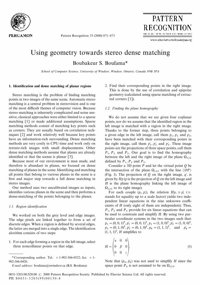
Consider a 3D point P and let the virtual point Q bethe intersection of the plane )

123with the line SOPT

(Fig. 1). The projection of Q on the right image, q@, isgiven by Hp (p is the projection of Q on the left image andH is the plane homography linking the left image of)

123to its right image).

For each couple (pi, p@

i), the relation Hp

iKp@

i(K

stands for equality up to a scale factor) yields two inde-pendent linear equations in the nine unknown coe$-cients of H (only eight of them are independent). Thus,P1, P

2and P

3provide for six linear equations that can

be used to constrain and simplify H. By using two par-ticular coordinate systems in the two images such that:p1"(0, 0, 1)T, p@

1"(0, 0, 1)T, p

2"(1, 0, 0)T, p@

2"(1, 0, 0)T,

p3"(0, 1, 0)T, p@

3"(0, 1, 0)T, p

4"(1, 1, 1)T, and p@

4"

(1, 1, 1)T, H simpli"es to

H"Aa 0 0

0 b 0

0 0 cB. (1)

Note that (p4, p@

4) was not used to simplify H since the

space point P4

is not assumed to be on )123

.

0031-3203/00/$20.00 ( 2000 Pattern Recognition Society. Published by Elsevier Science Ltd. All rights reserved.PII: S 0 0 3 1 - 3 2 0 3 ( 9 9 ) 0 0 1 5 0 - 8

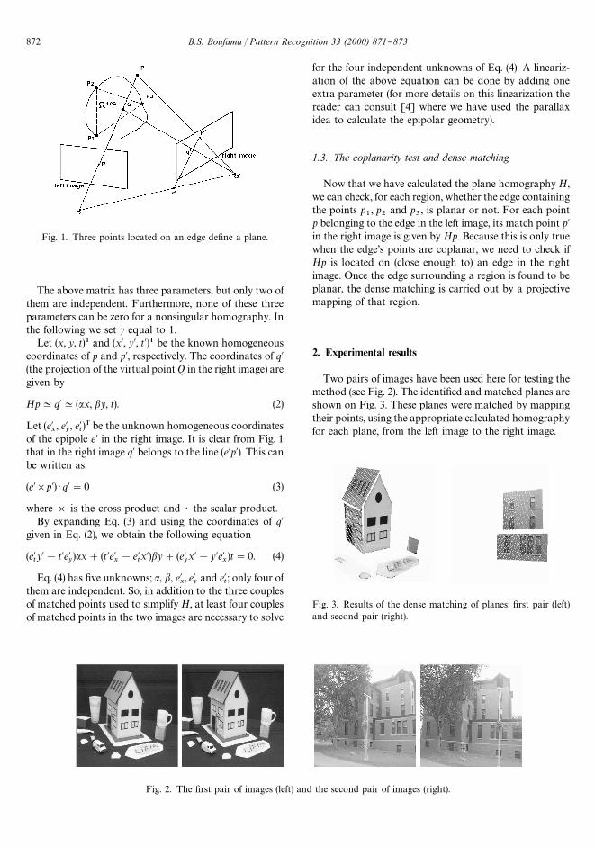
Fig. 2. The "rst pair of images (left) and the second pair of images (right).

Fig. 1. Three points located on an edge de"ne a plane.

Fig. 3. Results of the dense matching of planes: "rst pair (left)and second pair (right).

The above matrix has three parameters, but only two ofthem are independent. Furthermore, none of these threeparameters can be zero for a nonsingular homography. Inthe following we set c equal to 1.

Let (x, y, t)T and (x@, y@, t@)T be the known homogeneouscoordinates of p and p@, respectively. The coordinates of q@(the projection of the virtual point Q in the right image) aregiven by

HpKq@K(ax, by, t). (2)

Let (e@x, e@

y, e@

t)T be the unknown homogeneous coordinates

of the epipole e@ in the right image. It is clear from Fig. 1that in the right image q@ belongs to the line (e@p@). This canbe written as:

(e@]p@) ) q@"0 (3)

where ] is the cross product and ) the scalar product.By expanding Eq. (3) and using the coordinates of q@

given in Eq. (2), we obtain the following equation

(e@ty@!t@e@

y)ax#(t@e@

x!e@

tx@)by#(e@

yx@!y@e@

x)t"0. (4)

Eq. (4) has "ve unknowns; a, b, e@x, e@

yand e@

t; only four of

them are independent. So, in addition to the three couplesof matched points used to simplify H, at least four couplesof matched points in the two images are necessary to solve

for the four independent unknowns of Eq. (4). A lineariz-ation of the above equation can be done by adding oneextra parameter (for more details on this linearization thereader can consult [4] where we have used the parallaxidea to calculate the epipolar geometry).

1.3. The coplanarity test and dense matching

Now that we have calculated the plane homography H,we can check, for each region, whether the edge containingthe points p

1, p

2and p

3, is planar or not. For each point

p belonging to the edge in the left image, its match point p@in the right image is given by Hp. Because this is only truewhen the edge's points are coplanar, we need to check ifHp is located on (close enough to) an edge in the rightimage. Once the edge surrounding a region is found to beplanar, the dense matching is carried out by a projectivemapping of that region.

2. Experimental results

Two pairs of images have been used here for testing themethod (see Fig. 2). The identi"ed and matched planes areshown on Fig. 3. These planes were matched by mappingtheir points, using the appropriate calculated homographyfor each plane, from the left image to the right image.

872 B.S. Boufama / Pattern Recognition 33 (2000) 871}873

References

[1] Z. Zhang, R. Deriche, O.D. Faugeras, Q.T. Luong, A robusttechnique for matching two uncalibrated images through therecovery of the unknown epipolar geometry, Artif. Intell. 78(1}2) (1994) 87}119.

[2] P. Aschwanden, W. GuggenbuK hl, Experimental results froma comparative study on correlation type registration algorithms,in: FoK rstner, Ruwiedel (Eds.), Robust Computer Vision,Wichmann Verlag, Heidelberg, Germany, 1992, pp. 268}282.

[3] P. Meer, S. Ramakrishna, R. Lenz, Correspondenceof coplanar features through p2-invariant representations,in: Proceedings of the 12th International Conferenceon Pattern Recognition, Jerusalem, Israel 1994, pp. A-196}202.

[4] B. Boufama, R. Mohr, Epipole and fundamental matrixestimation using the virtual parallax property, in: Proceed-ings of the 5th International Conference on ComputerVision, Cambridge, Massachusetts, USA June 1995,pp. 1030}1036.

B.S. Boufama / Pattern Recognition 33 (2000) 871}873 873