using garch-in-mean model to investigate volatility and ...store.ectap.ro/articole/721.pdf · using...

Using Garch-in-Mean Model to Investigate Volatility and Persistence

55


at Different Frequencies for Bucharest Stock Exchange during 1997-2012

Iulian PANAIT Bucharest Academy of Economic Studies

[email protected] Ecaterina Oana SLĂVESCU

Bucharest Academy of Economic Studies [email protected]

Abstract. In our paper we use data mining to compare the

volatility structure of high (daily) and low (weekly, monthly) frequencies for seven Romanian companies traded on Bucharest Stock Exchange and three market indices, during 1997-2012. For each of the 10 time series and three frequencies we fit a GARCH-in-mean model and we find that persistency is more present in the daily returns as compared with the weekly and monthly series. On the other hand, the GARCH-in-mean failed to confirm (on our data) the theoretical hypothesis that an increase in volatility leads to a rise in future returns, mainly because the variance coefficient from the mean equation of the model was not statistically significant for most of the time series analyzed and on most of the frequencies. The diagnosis that we ran in order the verify the goodness of fit for the model showed that GARCH-in-mean was well fitted on the weekly and monthly time series but behaved less well on the daily time series.

Keywords: stock returns; volatility; persistence; GARCH model; emerging markets; data mining. JEL Codes: G01, G11, G12, G14, G15, G17, G32. REL Code: 11B.

Theoretical and Applied Economics Volume XIX (2012), No. 5(570), pp. 55-76

Iulian Panait, Ecaterina Oana Slăvescu

56

1. Introduction Stock markets, in particular, and financial markets, in general, are well

known for their uncertainty. Prices of stocks, bonds, commodities, all kind of traded financial derivatives, as well as interest rates and exchange rates are prone to constant variability. As a result of this variability, their returns over different periods of time are significantly volatile and difficult to forecast.

Volatility was always considered to be a key variable for assessing the condition of the financial markets and for making decisions by investors, speculators, investment managers and financial regulators. In the actual context of the years 2007-2012, characterized by a continuing financial and economic crisis, terms such as volatility forecast and risk management are very often mentioned by the scientific community and experienced top practitioners all around the world.

With time, researchers proposed many and diverse models to forecast volatility, ranging from time series based volatility models (exponential smoothening, Garman-Klass, Autoregressive Conditional Heteroscedasticity etc.) to option market implied volatility models. Also, the empirical performance of such models was investigated by many authors and for many local financial markets. Bollerslev (1986, pp. 307-327) used ARMA and EGARCH models to study US stocks from 1889 to 1990; Akigray (1989, pp. 55-80) tested GARCH(1,1), ARCH(2) and EWMA in order to identify the time series properties of US stock returns; McMillan and Gwilym (2000, pp. 438-448) investigated the performance of Random Walk, Moving Average, Exponential Smoothen, EMWA, GARCH(1,1), TGARCH(1,1), EGARCH(1,1) and FIGARCH(1,1) for stocks traded on London Stock Exchange; Franses and Djik (1998: pp.229-235) compared volatility forecasts of QGARCH(1,1), GJR-GARCH(1,1), GARCH(1,1) and Random Walk for stock indices in Spain, Germany, Italy, Netherland and Sweden; Harque et all (2004, pp. 19-42)) tested Random Walk, ARMA and GARCH-M models for ten Middle East and African emerging markets.

Also, regarding the behavior of volatility for companies listed on Bucharest Stock Exchange there were previous tests of symmetrical and asym-metrical GARCH models done by Lupu (2005, pp. 47-62, 2007, pp. 19-28), Tudor (2008, pp. 183-208) and Miron (2010, pp. 74-93). In their researches, the three Romanian authors used daily data (mainly for Bucharest Stock Exchange BET index) in order to estimate different GARCH models, with the parameters and settings. Their main aim was to test the validity of those models and to find the model that better fitted the particularities of returns for Romanian market.


57

In our paper we will investigate one very popular model from the GARCH family: the GARCH-in-mean model. Our choice for this model is motivated by the conclusion of previous related studies: the fact that in the financial markets risk and the expected return are correlated, and as a result of that, in the mean equation of the GARCH model there should be a reference to variance.

Our new and original contribution to the current state of research in this field is represented by three facts: (1) we calibrate the GARCH-M model not only to daily but also to weekly and monthly data; (2) in order to gain more significance for the results, we use a larger group of Romanian assets than the previous authors did, as we include in the research three market indices and seven among the most liquid listed companies; and finally, (3) we compare the values for the coefficients at different frequencies in order to see how the persistence of past shocks in mean and volatility change with time structure of the series.

To cast some light on these issues, the rest of the paper is organized as follows: section 2 presents the most relevant Romanian and international related studies; section 3 describes the data that we worked with and the data mining methodology that we have used; section 4 presents the results that we have obtained; finally section 5 summarizes the most important conclusions and proposes further studies in this field.

2. Literature review Before the scientific community became focused on heteroscedasticity

and its effects on forecasting and investment decision, researchers frequently used the Autoregressive Integrated Moving Average (ARIMA) model developed by Box and Jenkins (1976) in order to asses volatility of financial assets. Also the Black and Scholes (1975, pp. 307-324) equations for option pricing were used to determine implied volatility. These approaches are based on the erroneous hypothesis of constant variance for the time series of financial returns. As a result they failed to capture the “stylized facts” (Cont, 2001, pp. 223-236) of financial returns such as: leptokurtosis, volatility clustering, intermittency, fat tails, leverage effect etc.

In order to accommodate the empirical observation that variance is variable with time and that it seems dependent on past values, Engle (1982, pp. 987-1008) proposed the Autoregressive Conditional Heteroscedasticity (ARCH) models where variance is dependent on previous squared errors. Eagle’s model successfully addressed the above mentioned issues of financial time series but its coefficients are difficult to estimate. Bollerslev (1986,


58

pp. 307-327) proposed a generalization of the ARCH model in which variance depends simultaneously on the squared residuals and on its own past values. It is important to mention that unlike other models, ARCH and GARCH estimate coefficients via the maximum likelihood procedure, instead of using the sample standard deviation.

The modeling of financial time series with ARCH and GARCH models received much attention in the scientific community. Bollerslev et al. (1992, pp. 5-59) realized an overview of more than 300 relevant references at that time, but more valuable research in this field continued to be made since then.

Rizwan and Khan (2007, pp. 362-375) studied the volatility of the Pakistani stock market and found volatility clustering. Dawood (2007) investigated volatility in the Karachi Stock Exchange and found that in 1990’s the market has become more volatile on short and medium term (daily and monthly basis).

Chang (2006) investigated the mean reversion behavior of different series of data and concluded that mean reversion situation exists in the low-frequency data but not in the high-frequency data. Caiado (2004) found the same results by using GARCH models on the Portuguese Stock Index PSI20.

Selcuk (2004) investigated volatility in emerging stock markets and found volatility persistency. Magnus and Fosu (2006, pp. 2042-2048) found the parameter estimates of GARCH models for Ghana Stock Exchange close to unity which suggests a high level of persistence.

Donaldson and Kamstra (1997, pp. 17-46) find important differences in volatility between international markets, such as significant persistence of volatility effects in Japan relative to European and North American coutries.

Nam, Pyun and Arize (2002, pp. 563-588) use asymmetric GARCH-M model for US market indices during 1926-1997 and find that negative returns on average reverted more quickly to the long term average that the positive returns.

Lupu (2005) tested a GARCH model on the main index of Bucharest Stock Exchange and found that the model manages to catch the stylized facts of the local stock market. Also, Lupu and Lupu (2007) employed a EGARCH model for the same index of the Romanian Stock Market.

Tudor (2008) used GARCH and GARCH-M models for Romanian and US market’s main indices and found that the GARCH-M model performs better and confirms that there is a correlation between volatility and expected returns on both markets.

Miron and Tudor (2010) estimated different asymmetric GARCH family models (EGARCH, PGARCH and TGARCH) specifying successively a Normal, Student’s t and GED error distribution. They found that EGARCH


59

with GED and Student’s t errors are more accurate in the Romanian stock market.

In this paper we continue the work of previously mentioned Romanian authors by investigating the performance of GARCH-M model on a larger number of Romanian assets and also by taking into consideration lower frequencies of data (weekly and monthly time series) in addition to the daily returns already studied by those authors. We are interested to understand how persistence behaves on lower frequencies data.

3. Data and methodology For our study we have selected the most popular, diversified and relevant

three Bucharest Stock Exchange market indices: BET, BET-XT and BET-C. Also, we have selected seven of the most liquid companies (the list with their name and market symbol is presented in Table 1 at the end of this article).

For all those seven companies and for the three market indices we have obtained official daily stock prices during the period September 1997 – January 2012. The data were provided by the Bucharest Stock Exchange itself, courtesy of the Trading Department.

We were very careful to adjust all the prices with the corporate events that took place during the investigated period for some of the companies included in our study (mainly dividends and share capital increases). The price time series for three market indices was already adjusted with corporate events by the stock exchange as part of the official index calculation methods.

As we are not making correlation analysis between the companies or indices, there was no need to align the series in perfect synchronous chronologic order. This allowed us to keep in our analysis companies that were not actually traded during the whole period. The Table 1 presented at the end of this article includes information regarding the actual period and the number of daily, weekly and monthly observations for each company.

After all this preparations were accomplished, in order to eliminate the obvious non-stationarity from our data, we have transformed the price time series into return time series for all the seven individual stocks and for the three indices.

Regarding the returns estimation, as Strong (1992, p. 353) pointed out “there are both theoretical and empirical reasons for preferring logarithmic returns. Theoretically, logarithmic returns are analytically more tractable when linking together sub-period returns to form returns over long intervals. Empirically, logarithmic returns are more likely to be normally distributed and so conform to the assumptions of the standard statistical techniques.” This is


60

why we decided to use logarithmic returns in our study since one of our objectives was to test of whether the daily returns were normally distributed or, instead, showed signs of asymmetry (skewness). The computation formula of the daily returns is as follows:

1t,i

t,it,i P

PLnR

where Ri,t is the return of asset i in period t; Pi,t is the price of asset i in period t and Pi,t-1 is the price of asset i in period t-1. As already mentioned above, according to this methodology of computing the returns, the prices of the assets must be adjusted for corporate events such as dividends, splits, consolidations and share capital increases (mainly in case of individual stocks because indices are already adjusted).

As a result of this initial data gathering we obtained 10 time series of log-

returns for each investigated frequency: daily, weekly and monthly: in total there are 30 time series.

Before estimating the GARCH-in-mean model, we investigated all the data series, for all the frequencies, in order to identify their statistical properties and to see if they meet the pre-conditions for the GARCH-in-mean model.

The first step in this direction was to examine the descriptive statistics for the 10 time series, at each frequency. The results are presented in tables 2, 3 and 4 at the end of this article. From these tables we draw 4 important conclusions:

(1) First we can observe that average returns for all the time series and all frequencies present very low values and that the values for standard deviation are in all cases significantly larger than mean values. Further statistical tests show that we cannot reject the null hypothesis of zero mean for none of the time series or frequency. This finding will prove very important latter when we will apply the GARCH-M model.

(2) Second, we can observe that standard deviations of the series of monthly returns are higher than the standard deviations for the weekly and daily returns series. Also, the standard deviations of the weekly returns series are higher in comparison with the standard deviations of the daily return series. This is a common feature of financial assets.

(3) Most of the time series, under all the three frequencies, present negative skewness. Also, all the time series, under all the three frequencies, present excess kurtosis and fat tails. This is another common feature of financial assets.

(4) None of the 10 time series studied are normally distributed, for none of the three frequencies investigated, as proven by values for the Jarque-Bera tests shown in tables 2, 3 and 4.


61

Going further with our preliminary investigation of the data sample, we compute the squared returns for all the 10 time series under all the three frequencies and test for evidence of heteroscedasticity and volatility clustering. Our special interest for the squared returns come from the fact mentioned previously (and extensively documented by other related studies) that we can’t reject the hypothesis that the average of the daily, weekly and monthly returns is different from zero. If we assume that the mean is zero, than the unconditional variance can be approximated by the square return of that particular day, week or month.

The clustering of volatility can be observed from the simple graphics of the squared returns as presented in figures 1, 2 and 3 shown at the end of this article. This particular stylized fact of financial asset returns is more present in the daily and weekly time series and from our data it seems less present in the monthly time series.

We investigate the heteroscedasticity of the 10 time series, for all the three frequencies, by calculating the autocorrelation (AC) and partial autocorrelation (PAC) functions, and also by performing the Ljung-Box Q-statistics. In all our calculations we used a 20 period lag. The results are presented in Table 5 shown at the end of this article. We observe the presence of serial correlation till the 20-th lag for all the daily time series and for most of the weekly time series (with the notable exception of weekly returns for BRD), as indicated by the AC and PAC values and also by the p-value of the Q-test lower than 1%. Also it is extremely important to notice that the p-value of the Q-test is higher than 1% for all the monthly time series which means that we can’t reject the null hypothesis of inexistence of serial correlation for none of them. To summarize: we find heteroscedasticity in the daily returns and in most of the weekly returns. However we can’t confirm the presence of heteroscedasticity in the weekly returns of BRD and also in none of the monthly returns. Since heteroscedasticity is a pre-condition for applying the GARCH models to a financial time series, we might be unable to fit such a GARCH model on the monthly returns and also on the weekly returns of BRD.

After all these preliminary investigation of the data sample were concluded, we continued with the actual estimation of the parameters of the GARCH-in-mean model for all the time series and all the data frequencies. The GARCH-in-mean model was developed by Engle, Lilien and Robins (1987), it is based on the GARCH(1,1) model introduced by Bollerslev (1986, pp. 307-327), and it consists of two equations, one for the mean and another one for the variance of the time series:

the mean equation: i211iR

the variance equation: 21i

21i

21


62

4. Results and interpretations The data from Table 6 presented at the end of this article show the values

for the β1, ω, α and β coefficients of the GARCH-M model for all the time series and frequencies. It is important to mention that in all our estimates of the model we used the hypothesis that the errors are normally distributed. There are several conclusions that can be drawn from this table:

(1) First, we can observe that with only one exception (the daily time series for BET-C index) the estimated coefficients of the model respect the requirement that (α + β)<1, which is a crucial condition for a mean reverting process. This enables us to conclude that conditional volatilities are mean reverting for all the time series and frequencies, except in case of the daily returns for BET-C index.

(2) Second, we can observe that the case of most time series and frequencies, the estimated coefficients for the variance equation of the model (the ω, α and β coefficients) are statistically significant at the 90% confidence level. Most of them are statistically significant even at the 99% confidence level. The only notable exception is the monthly time series for AZO, where at the 90% confidence level we are not able to reject the null hypothesis that coefficients of the variance equation are zero.

(3) Third conclusion and an extremely important one for our study is that, with only four exceptions, the β1 coefficient for the variance term in the mean equation is not statistically significant. This practically invalidates our initial hypothesis that there is correlation between risk and expected return. If that hypothesis was to be true, we should have found p-values of less the 0.1 for all (or at least most of) the Z-tests of significance for these coefficients in all our time series and frequencies. In practical terms we can conclude that our GARCH-M model applied to our daily, weekly and monthly data for Bucharest Stock Exchange during 1997-2012 failed to show a statistically significant correlation between risk and expected return. The only exceptions are the weekly and monthly time series for BET-FI, the daily time series for CMP and the weekly time series for BIO where we found that the β1 coefficients are statistically significant at the 90% confidence level.

The latter conclusion above tells us that other models in the GARCH(1,1) family should be better for modeling and forecasting volatility behavior in the Romanian Stock Market.

Even if the GARCH-M model failed to prove appropriate, the GARCH(1,1) is correctly specified and validated by our results, which enables us to continue our investigation of the behavior of volatility persistence (or mean reverting) in different frequencies of data. In order to move forward with


63

this objective of our research, we have computed and presented in Table 7 (shown at the end of this article) the persistence coefficients (calculated as sum of the α and β coefficients) for all the time series and frequencies except the for the monthly time series of returns for AZO, BET-FI and SIF2 where our previous results showed that at least one of those coefficients from the variance equation of the model are not statistically significant. The values from Table 7 converge to the following important conclusions:

(1) First, as we have noticed earlier, since the persistence coefficient of the daily time series for BET-C is above 1 we can conclude that this process is not mean reverting but rather explosive.

(2) Second, in seven out of 10 cases the weekly conditional volatilities of returns tend to revert faster towards the mean in comparison with the daily conditional volatilities. Also, in six out of seven cases where the monthly persistence coefficients were statistically significant, they showed that the monthly conditional volatilities of returns tend to revert faster towards the mean in comparison with the daily conditional volatilities.

(3) Third, in four in out of seven cases where the monthly persistence coefficients were statistically significant, they showed that the monthly conditional volatilities of returns tend to revert faster towards the mean in comparison with the weekly conditional volatilities.

Over all, from the last two observations mentioned above, we can argue that our use of the GARCH model for characterizing conditional volatility at different time frequency in three indices and seven companies traded on Bucharest Stock Exchange during 1997-2012 leads us to the conclusion that often (in most cases) the conditional volatilities tend to revert faster towards the long term average for lower frequencies of data in comparison with higher frequencies of data. In particular we found that in most cases the monthly conditional volatilities of returns tend to revert faster towards the long term average than the weekly and daily conditional volatilities, and also that the weekly conditional volatilities of returns tend to revert faster towards the long term average than the daily conditional volatilities.

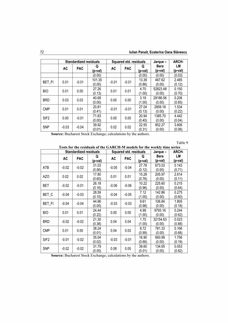
In order for our conclusions to be credible, we needed to fulfill one more step in the data analysis: we needed to diagnose the goodness of fit of the GARCH models in all the cases by looking into the properties of the residuals and squared residuals of each particular case. In order to do that we did the following tests for each model fitted:

(1) First we investigated the autocorrelation (AC) and partial correlation (PAC) of the standardize residuals till the 20-th lag, and also we performed the Ljung-Box Q-statistics at the 20th lag to see if there is evidence of autocorrelation of the standardized residuals.


64

(2) Second we investigated the autocorrelation (AC) and partial correlation (PAC) of the squared standardized residuals till the 20-th lag, and also we performed the Ljung-Box Q-statistics at the 20th lag to see if there is evidence of autocorrelation of the squared standardized residuals.

(3) Third we employed the Jarque-Bera test in order to conclude if the residuals are normally distributed or not.

(4) Fourth we calculated the statistics of the ARCH-LM test in order to detect posible remaining ARCH effects among the residuals with the help of the Lagrange Multiplier.

The tables 8, 9 and 10 presented at the end of this article show the results of these investigations into the goodness of fit of the GARCH models that we employed over the specified time series at different frequencies.

From the data presented in Tables 9 and 10 we can conclude that the GARCH model that we used to characterize volatility of the weekly and monthly time series fitted very well, because the AC, PAC and Q statistics show that there is no statistically significant trace of autocorrelation left in the standardized and squared standardized residuals. Also, the ARCH-LM tests show that there is no statistically significant trace of ARCH effect left in the residuals. None of the residuals are normally distributed, but this often happens for the residuals of the models applied to financial time series.

The data presented in Table 8 shows a different little different picture regarding the residuals from the daily time series: (1) the ARCH-LM test proves that there is no statistically significant trace of ARCH effect left in the residuals (with the exception of the time series for BET index) which is a positive outcome for us; (2) also squared standardized residuals don’t show statistically significant autocorrelation till the 20-th lag (with the exception of the time seris for BET-C index); (3) unfortunately five out of the 10 daily time series of standardized residuals still present statistically significant signs of autocorrelation (at the 99% confidence level); (4) as in the case of monthly and weekly data, none of the residuals are normally distributed.

Over all, taking into account the conclusions drawn from tables 8,9 and 10 we conclude that the GARCH-M models that we use are well fitted on the weekly and mothly data and as a consequence the results that we have obtained for these frequencies are statistically relevant. In general the results for the daily frequency can be considered relevant but with a lower quality since the tests showed that we should continue to test other models from the GARCH family because the GARCH-M didn’t manage to eliminate all the heteroscedasticity from the daily standardized residuals (although it succeded to eliminate all ARCH effects from the same residuals).


65

5. Conclusions In this paper we use the GARCH-in-mean model to characterize volatility

on Bucharest Stock Exchange for three different frequencies: daily, weekly and monthly. We use data for three market indices and seven of the most liquid companies during 1997-2012.

Most of the 10 time series used, under all the three frequencies mentioned, present the characteristics of heteroscedasticity and volatility clustering required in order to apply the GARCH(1,1) family of models.

After fitting, the model succeeded to eliminate all traces of statistically significant autocorrelation and ARCH effect from the resulted residuals of the weekly and monthly series. Also, the model succeeded to extract all signs of statistically significant ARCH effect from the residuals of the daily series, the squared standardized residuals from these series presented no statistically significant traces of autocorrelation, but the simple standardized residuals of the same series continued to show autocorrelation. None of the residuals from neither of the three frequencies were normally distributed. All these observations conducted us to the conclusions that the GARCH-in-mean model fitted well on our monthly and weekly data, but less well on the daily data where probably we should continue the research for a better model to characterize the evolution of the volatility.

In the great majority of the time series and frequencies the coefficients from the variance equation of the model proved to be statistically significant and they proved that conditional volatility tends to revert to the long term average (with only a single exception).

An important result of our research was that the variance coefficient from the mean equation of the model was not statistically significant for most of the series and frequencies. This finding leaded us to the conclusion that we can’t statistically prove on our data a clear correlation between risk and future returns, as considered in theory by many authors.

Another important result of our research was that in most of the cases we found that conditional volatility on the monthly time series tends to revert faster towards the long term average in comparison with the conditional volatility from the weekly and daily time series. Also, the persistence of the weekly conditional volatility was lower in comparison with the daily conditional volatility which means that the weekly conditional volatility tends to revert faster towards the long term average in comparison with the daily conditional volatility. These findings represent the most important original contribution of our research because such behavior was not previously investigated and


66

documented for the Romanian stock market by other authors, especially on such a large number of liquid assets.

The research on volatility persistence behavior, at different frequencies, of the Bucharest Stock Exchange should be continued by fitting other models from the GARCH family, especially asymmetrical models.

Acknowledgements This article is a result of the project POSDRU/88/1.5./S/55287 „Doctoral

Program in Economics at European Knowledge Standards (DOESEC)". This project is co-funded by the European Social Fund through The Sectorial Operational Program for Human Resources Development 2007-2013, coordinated by Bucharest Academy of Economic Studies in partnership with West University of Timisoara.

References Akigray, V., “Conditional Heteroscedasticity in Time of Stock Returns: Evidence and

Forecasting”, Journal of Business, no. 62, 1989, pp. 55-80 Black, F., Scholes, M., “Asset Speculative Prices”, Journal of Business, no. 7, 1975, pp. 307-324 Bollerslev, T., “Generalized Autoregressive Conditional Heteroscedasticity”, Journal of

Econometrics, no. 31, 1986, pp. 307-327 Bollerslev, T., Chou, R.Y., Kroner, K.F., “ARCH Modeling in Finance: a Review of the Theory

and Empirical Evidence”, Journal of Econometrics, no. 52, 1992, pp. 5-59 Box and Jenkins, (1976). Time Series Analysis and Control, 2nd edition, Holden Day, San

Francisco Cont, R., “Empirical properties of asset returns: stylized facts and statistical issues”,

Quantitative Finance, vol. 1, no. 2, 2001, pp. 223-236 Engle, R.F., “Autoregressive Conditional Heteroscedasticity with Estimates of the Variance of

the United Kingdom Inflation”, Econometrica, no. 5, 1982, pp. 987-1008 Franses, P.H., Djik, V.D., “Forecasting Stock Market Volatility Using Nonlinear GARCH”,

Journal of Forecasting, no. 15, 1998, pp. 229-235 Harque, M., Hassan, M.K., Maroney, N.C., Sackley, W.H., “An Empirical Examination of

Stability, Predictibility and Volatility of Middle Eastern and African Emerging Stock Markets”, Reviews of Middle East Economics and Finance, no. 2, 2004, pp. 19-42

Lupu, R., “Applying GARCH Model for Bucharest Stock Exchange BET index”, The Romanian Economic Journal, no. 17, 2005, pp. 47-62

Lupu, R., Lupu, I., “Testing for Heteroscedasticity on the Bucharest Stock Exchange”, The Romanian Economic Journal, no. 23, 2007, pp. 19-28

McMillan, S., Gwilym, M., “Forecasting United Kingdom’s Stock Markets Volatility”, Applied Financial Economics, no. 57, 2000, pp. 438-448


67

Miron, D., Tudor, C., “Asymmetric Conditional Volatility Models: Empirical Estimation and Comparison of Forecasting Accuracy”, Romanian Journal of Economic Forecasting, no. 3/2010, 2010, pp. 74-93

Peiró, A., “Skewness in Financial Returns”, Journal of Banking and Finance, no. 23, 1999, pp. 847–862

Peiró, A., “Skewness in Individual Stocks at Different Frequencies”, IVIE working papers, Instituto Valenciano de Investigaciones Economicas, WP-EC 2001-07: V-1486-2001

Strong, N., “Modeling Abnormal Returns: A Review Article”, Journal of Business Finance and Accounting, vol. 19, no. 4, 1992, pp. 533–553

Tudor, C., “Modeling time series volatilities using symmetrical GARCH models”, The Romanian Economic Journal, no. 30, 2008, pp. 183-208

Rizwan, M.F., Khan, S., “Stock Return Volatility in Emerging Equity Market (Kse): The Relative Effects of Country and Global Factors”, Int. Rev. Bus. Res. Papers, no. 3(2), 2007, pp. 362 - 375.

Selcuk, F., (2004), “Asymmetric Stochastic Volatility in Emerging Stock Markets”, Unpublished Research Paper

Dawood, M., “Macro Economic Uncertainty of 1990s and Volatility at Karachi Stock Exchange”, Munich Personal RePEc Archive (MPRA), Paper No. 3219, 2007

Caiado, J., “Modelling and forecasting the volatility of the Portuguese stock index PSI-20”, Munich Personal RePEc Archive (MPRA), Paper No. 2304, 2004

Chang., CH., (2006). “Mean Reversion Behavior of Short-term Interest Rate Across Different Frequencies,” Unpublished Research

Magnus, F.J., Fosu, A.E., “Modelling and Forecasting Volatility of Returns on the Ghana Stock Exchange Using Garch Models”, Am. J. Appl. Sci., no. 3(10), 2006, pp. 2042-2048

Donaldson, R.G., Kamstra, M., “An Artificial Neural Network - GARCH Model for International Stock Return Volatility”, Journal of Empirical Finance, no. 4(1), 1997, pp. 17-46.

Nam, K., Pyun, C.S., Arize, C.A., “Asymmetric mean-reversion and contrarian profits: ANST-GARCH approach”, Journal of Empirical Finance, vol. 9, no. 5, 2002, pp. 563-588


68

Table 1 The financial time series studied in this article

Series symbol Company name Number of observations March 2010 – March 2012

Daily Weekly Monthly BET Bucharest Stock Exchange BET index 3579 740 173 BET_C Bucharest Stock Exchange BET-C index 3441 711 166 BET_FI Bucharest Stock Exchange BET-FI index 2793 579 135 ATB Sc Antibiotice Sa Iasi 3579 740 173 AZO Sc Azomures Sa Tg. Mures 3579 740 173 BIO Sc Biofarm Sa Bucuresti 3579 740 173 BRD Sc Banca Romana de Dezvoltare – GSG Sa 2747 568 133 CMP Sc Compa Sa Sibiu 3579 740 173 SIF2 Societatea de Investitii Financiare Moldova Sa 3045 631 147 SNP Sc Petrom Sa – Group OMV 2585 535 125

Source: Bucharest Stock Exchange; calculations by the authors.

Table 2 Descriptive statistics for the daily time series

Mean Std. Dev. Skewness Kurtosis Jarque-Bera Probability ATB -0.0002 0.0320 -0.45 10.86 9331.5 0.00 AZO 0.0005 0.0387 0.10 9.25 5829.8 0.00 BET 0.0004 0.0187 -0.36 9.13 5691.4 0.00 BET_C 0.0003 0.0169 -0.49 16.02 24451.7 0.00 BET_FI 0.0011 0.0268 -0.12 8.11 3047.7 0.00 BIO 0.0001 0.0374 -0.14 14.43 19507.5 0.00 BRD 0.0005 0.0255 -0.85 12.66 11009.8 0.00 CMP 0.0003 0.0357 -0.15 8.06 3827.6 0.00 SIF2 0.0013 0.0348 -0.25 10.42 7019.6 0.00 SNP 0.0006 0.0272 -0.22 9.50 4576.9 0.00


Table 3 Descriptive statistics for the weekly time series

Mean Std. Dev. Skewness Kurtosis Jarque-Bera Probability ATB -0.0008 0.0829 -0.69 21.49 10598.7 0.00 AZO 0.0026 0.0914 0.39 8.09 817.4 0.00 BET 0.0021 0.0454 -0.30 6.44 376.7 0.00 BET_C 0.0014 0.0402 -0.67 6.45 404.4 0.00 BET_FI 0.0053 0.0639 -0.78 8.85 885.1 0.00 BIO 0.0006 0.0840 -0.89 12.14 2674.4 0.00 BRD 0.0026 0.0592 -2.32 22.60 9602.0 0.00 CMP 0.0016 0.0804 -0.02 9.26 1206.8 0.00 SIF2 0.0063 0.0852 0.46 18.82 6606.5 0.00 SNP 0.0029 0.0630 -0.57 14.58 3017.3 0.00



69

Table 4 Descriptive statistics for the monthly time series

Mean Std. Dev. Skewness Kurtosis Jarque-Bera Probability ATB -0.0036 0.1788 -1.22 10.98 501.9 0.00 AZO 0.0109 0.1988 1.93 18.56 1851.1 0.00 BET 0.0089 0.1107 -0.66 5.50 57.8 0.00 BET_C 0.0062 0.0997 -0.85 5.50 63.4 0.00 BET_FI 0.0228 0.1671 -0.54 8.68 188.2 0.00 BIO 0.0026 0.1918 -0.16 5.93 62.8 0.00 BRD 0.0113 0.1412 -1.50 9.27 268.1 0.00 CMP 0.0067 0.1834 -0.97 11.48 545.8 0.00 SIF2 0.0272 0.1902 -0.75 7.75 152.0 0.00 SNP 0.0123 0.1434 -0.85 8.76 188.1 0.00


Table 5 Estimation of the autocorrelation (AC), partial autocorrelation (PAC)

and Q-statistic with 20 lags for the squared returns with daily, weekly and monthly frequency

Daily time series Weekly time series Monthly time series

AC PAC Q

(p-val) AC PAC Q

(p-val) AC PAC Q

(p-val)

ATB 0.031 -0.026 1810.6 (0.00) -0.012 -0.039

444.1 (0.00) -0.043 -0.021

25.7 (0.18)

AZO 0.099 -0.002 1341.0 (0.00) 0.183 0.062

367.7 (0.00) -0.036 -0.023

5.4 (1.00)

BET 0.061 -0.016 1366.5 (0.00) -0.026 -0.056

150.2 (0.00) -0.049 -0.024

32.3 (0.04)

BET_C 0.042 -0.022 1006.4 (0.00) 0.000 -0.024

163.4 (0.00) -0.078 -0.062

24.4 (0.23)

BET_FI 0.102 -0.052 2086.0 (0.00) 0.011 -0.011

153.9 (0.00) -0.069 -0.052

13.4 (0.86)

BIO 0.080 0.041 611.5 (0.00) 0.005 0.003

113.6 (0.00) -0.087 -0.044

28.3 (0.10)

BRD 0.044 -0.034 747.5 (0.00) 0.073 0.063

17.7 (0.61) -0.018 -0.003

12.2 (0.91)

CMP 0.066 -0.025 1322.1 (0.00) 0.071 0.087

108.4 (0.00) -0.036 -0.039

27.8 (0.11)

SIF2 0.098 0.000 3540.7 (0.00) 0.006 0.004

48.3 (0.00) -0.073 -0.068

20.0 (0.46)

SNP 0.057 -0.018 2530.5 (0.00) 0.032 0.008

170.5 (0.00) -0.075 -0.033

13.4 (0.86)



70

Table 6 Estimated values for the GARCH-M coefficients for the all frequencies

Coeff value

Std. error

Z statistic

p- val

Coeff value

Std. error

Z statistic

p- val

Coeff value

Std. error

Z statis-

tic

p- val

Daily frequency Weekly frequency Monthly frequency

ATB

β1 -0.105 0.773 -0.136 0.89 -0.657 0.473 -1.390 0.16 -0.524 0.502 -1.044 0.30

ω 0.000 0.000 24.379 0.00 0.000 0.000 6.216 0.00 0.005 0.002 2.485 0.01

α 0.128 0.006 22.472 0.00 0.220 0.026 8.401 0.00 0.386 0.102 3.801 0.00

β 0.847 0.004 191.215 0.00 0.760 0.023 32.815 0.00 0.564 0.095 5.970 0.00

AZO

β1 0.160 0.715 0.223 0.82 -0.156 0.623 -0.250 0.80 -20.736 15.981 -1.298 0.19

ω 0.000 0.000 15.527 0.00 0.001 0.000 6.390 0.00 0.005 0.003 1.626 0.10

α 0.086 0.004 20.538 0.00 0.202 0.023 8.981 0.00 0.006 0.004 1.392 0.16

β 0.882 0.005 195.961 0.00 0.721 0.027 26.611 0.00 0.869 0.075 11.577 0.00

BET

β1 0.719 1.242 0.579 0.56 -1.930 1.227 -1.572 0.12 -0.772 1.648 -0.468 0.64

ω 0.000 0.000 10.484 0.00 0.000 0.000 4.227 0.00 0.001 0.001 2.262 0.02

α 0.231 0.010 22.521 0.00 0.183 0.027 6.812 0.00 0.199 0.063 3.175 0.00

β 0.760 0.008 93.064 0.00 0.780 0.030 26.381 0.00 0.713 0.079 8.973 0.00

BET_C

β1 -0.448 1.123 -0.399 0.69 -2.516 1.610 -1.563 0.12 -1.559 1.710 -0.912 0.36

ω 0.000 0.000 10.197 0.00 0.000 0.000 4.443 0.00 0.002 0.001 2.134 0.03

α 0.233 0.010 22.452 0.00 0.223 0.035 6.306 0.00 0.371 0.127 2.927 0.00

β 0.770 0.008 96.036 0.00 0.680 0.046 14.877 0.00 0.447 0.158 2.832 0.00

BET_FI

β1 -0.079 1.120 -0.071 0.94 -2.986 1.062 -2.812 0.00 1.115 0.602 1.852 0.06

ω 0.000 0.000 7.157 0.00 0.000 0.000 4.528 0.00 0.004 0.004 1.255 0.21

α 0.166 0.011 14.677 0.00 0.223 0.042 5.359 0.00 0.154 0.046 3.320 0.00

β 0.823 0.010 85.738 0.00 0.675 0.049 13.669 0.00 0.693 0.163 4.260 0.00

BIO

β1 -1.164 0.658 -1.768 0.08 -0.282 0.907 -0.311 0.76 -0.266 0.939 -0.283 0.78

ω 0.000 0.000 36.499 0.00 0.000 0.000 6.812 0.00 0.006 0.003 2.125 0.03

α 0.181 0.007 27.111 0.00 0.106 0.019 5.520 0.00 0.206 0.089 2.324 0.02

β 0.750 0.006 132.280 0.00 0.833 0.022 37.480 0.00 0.647 0.137 4.735 0.00

BRD

β1 0.270 1.061 0.254 0.80 -1.200 2.115 -0.568 0.57 0.001 1.302 0.001 1.00

ω 0.000 0.000 22.541 0.00 0.002 0.000 6.750 0.00 0.002 0.001 2.324 0.02

α 0.277 0.016 16.888 0.00 0.217 0.051 4.247 0.00 0.164 0.060 2.747 0.01

β 0.663 0.014 46.275 0.00 0.323 0.099 3.265 0.00 0.722 0.054 13.349 0.00

CMP

β1 -0.181 0.798 -0.227 0.82 -2.117 1.026 -2.064 0.04 0.363 0.488 0.744 0.46

ω 0.000 0.000 15.477 0.00 0.001 0.000 4.258 0.00 0.004 0.002 2.217 0.03

α 0.210 0.013 16.777 0.00 0.144 0.024 5.890 0.00 0.180 0.031 5.737 0.00


71

Coeff value

Std. error

Z statistic

p- val

Coeff value

Std. error

Z statistic

p- val

Coeff value

Std. error

Z statis-

tic

p- val

Daily frequency Weekly frequency Monthly frequency

β 0.668 0.016 41.516 0.00 0.739 0.044 16.749 0.00 0.708 0.067 10.598 0.00

SIF2

β1 -0.792 0.796 -0.996 0.32 0.660 0.466 1.418 0.16 0.287 1.117 0.257 0.80

ω 0.000 0.000 10.184 0.00 0.001 0.000 7.262 0.00 0.008 0.005 1.564 0.12

α 0.149 0.009 15.934 0.00 0.127 0.020 6.309 0.00 0.275 0.069 4.002 0.00

β 0.824 0.008 101.628 0.00 0.754 0.028 26.812 0.00 0.532 0.160 3.326 0.00

SNP

β1 -0.101 1.104 -0.091 0.93 -0.636 1.050 -0.606 0.54 -0.057 1.145 -0.050 0.96

ω 0.000 0.000 10.321 0.00 0.001 0.000 4.750 0.00 0.002 0.001 2.558 0.01

α 0.158 0.011 13.867 0.00 0.250 0.050 4.970 0.00 0.302 0.066 4.562 0.00

β 0.798 0.012 66.686 0.00 0.514 0.075 6.842 0.00 0.648 0.048 13.531 0.00


Table 7

Persistence values for all the time series and frequencies Daily Weekly Monthly

ATB 0.9751 0.9803 0.9509 AZO 0.9677 0.9239 not significant BET 0.9906 0.9627 0.9112 BET_C 1.0033 0.9025 0.8181 BET_FI 0.9887 0.8987 not significant BIO 0.9308 0.9392 0.8531 BRD 0.9400 0.5399 0.8858 CMP 0.8779 0.8834 0.8890 SIF2 0.9734 0.8804 not significant SNP 0.9557 0.7641 0.9499


Table 8

Tests for the residuals of the GARCH-M models for the daily time series Standardized residuals Squared std. residuals Jarque –

Bera (p-val)

ARCH-LM

(p-val) AC PAC Q

(p-val) AC PAC

Q (p-val)

ATB -0.01 -0.01 29.91 (0.07) -0.02 -0.02

7.55 (0.99)

12775.27 (0.00)

1.147 (0.28)

AZO 0.03 0.02 23.40 (0.27) -0.01 -0.01

11.68 (0.93)

9688.15 (0.00)

4.333 (0.04)

BET 0.02 0.01 153.86 (0.00)

0.00 0.00 34.91 (0.02)

802.48 (0.00)

9.270 (0.00)

BET_C 0.01 0.00 140.23 -0.01 -0.02 40.96 2422.87 4.475


72

Standardized residuals Squared std. residuals Jarque – Bera

(p-val)

ARCH-LM

(p-val) AC PAC Q (p-val)

AC PAC Q (p-val)

(0.00) (0.00) (0.00) (0.03)

BET_FI 0.01 -0.01 101.35 (0.00) -0.01 -0.01

13.39 (0.86)

467.62 (0.00)

2.485 (0.12)

BIO 0.01 0.00 27.26 (0.13) 0.01 0.01

4.70 (1.00)

52823.48 (0.00)

0.150 (0.70)

BRD 0.03 0.03 40.68 (0.00)

0.00 0.00 3.19 (1.00)

29186.56 (0.00)

0.206 (0.65)

CMP 0.01 0.01 20.81 (0.41)

-0.01 -0.01 27.04 (0.13)

2859.18 (0.00)

1.534 (0.22)

SIF2 0.00 -0.01 71.83 (0.00)

0.00 0.00 20.94 (0.40)

1385.70 (0.00)

4.442 (0.04)

SNP -0.03 -0.04 39.92 (0.01) 0.02 0.02

22.55 (0.31)

852.27 (0.00)

3.606 (0.06)


Table 9 Tests for the residuals of the GARCH-M models for the weekly time series


(p-val)

ARCH-LM


AC PAC Q (p-val)

ATB -0.02 -0.02 31.03 (0.06)

-0.05 -0.04 27.78 (0.12)

673.03 (0.00)

0.143 (0.71)

AZO 0.02 0.02 17.80 (0.60) 0.01 0.01

15.28 (0.76)

205.97 (0.00)

2.614 (0.11)

BET -0.02 -0.01 26.18 (0.16) -0.06 -0.06

10.22 (0.96)

225.60 (0.00)

0.215 (0.64)

BET_C -0.04 -0.03 28.59 (0.10)

-0.04 -0.05 7.12 (1.00)

142.86 (0.00)

0.275 (0.60)

BET_FI -0.04 -0.04 44.96 (0.00)

-0.03 -0.03 9.61 (0.98)

106.84 (0.00)

1.805 (0.18)

BIO 0.01 0.01 24.44 (0.22)

0.00 0.00 4.99

(1.00) 9793.16 (0.00)

0.244 (0.62)

BRD -0.02 -0.02 21.30 (0.38)

0.04 0.04 1.70

(1.00) 32154.63

(0.00) 0.023 (0.88)

CMP 0.01 0.00 38.24 (0.01) 0.04 0.03

8.72 (0.99)

781.33 (0.00)

0.166 (0.68)

SIF2 -0.01 -0.02 35.04 (0.02) -0.03 -0.01

16.90 (0.66)

660.99 (0.00)

1.756 (0.19)

SNP -0.02 -0.02 31.79 (0.05)

0.08 0.05 39.60 (0.01)

134.65 (0.00)

0.053 (0.82)



73

Table 10 Tests for the residuals of the GARCH-M models for the monthly time series


(p-val)

ARCH-LM


AC PAC Q (p-val)

ATB 0.14 0.14 20.28 (0.44)

-0.02 -0.03 6.17 (1.00)

427.51 (0.00)

0.237 (0.63)

AZO 0.00 0.06 14.39 (0.81)

-0.03 -0.03 1.87

(1.00) 3138.06 (0.00)

0.039 (0.84)

BET -0.02 -0.04 15.66 (0.74) 0.04 0.08

15.27 (0.76)

23.97 (0.00)

0.109 (0.74)

BET_C -0.01 -0.02 13.75 (0.84) -0.01 -0.03

10.06 (0.97)

10.67 (0.00)

0.700 (0.40)

BET_FI 0.06 0.03 14.05 (0.83)

-0.05 -0.04 6.72 (1.00)

120.52 (0.00)

0.074 (0.79)

BIO 0.06 0.03 13.63 (0.85)

-0.09 -0.07 9.66 (0.97)

107.70 (0.00)

0.317 (0.57)

BRD 0.05 0.07 12.27 (0.91)

0.06 -0.02 18.04 (0.59)

29.01 (0.00)

0.406 (0.53)

CMP 0.01 0.05 35.62 (0.02)

-0.02 -0.02 14.45 (0.81)

46.65 (0.00)

2.348 (0.13)

SIF2 0.10 0.06 11.87 (0.92) -0.04 -0.04

6.73 (1.00)

59.90 (0.00)

0.021 (0.89)

SNP 0.05 0.02 12.17 (0.91) -0.07 -0.07

9.75 (0.97)

32.95 (0.00)

0.007 (0.94)



74

.00

.01

.02

.03

.04

98 00 02 04 06 08 10

_R2ATB

.00

.02

.04

.06

.08

.10

98 00 02 04 06 08 10

_R2AZO

.000

.004

.008

.012

.016

.020

98 00 02 04 06 08 10

_R2BET

.00

.01

.02

.03

.04

98 00 02 04 06 08 10

_R2BET_C

.000

.004

.008

.012

.016

.020

.024

.028

98 00 02 04 06 08 10

_R2BET_FI

.00

.02

.04

.06

.08

.10

98 00 02 04 06 08 10

_R2BIO

.00

.01

.02

.03

.04

.05

.06

98 00 02 04 06 08 10

_R2BRD

.00

.02

.04

.06

.08

.10

98 00 02 04 06 08 10

_R2CMP

.00

.02

.04

.06

.08

98 00 02 04 06 08 10

_R2SIF2

.000

.004

.008

.012

.016

.020

.024

.028

98 00 02 04 06 08 10

_R2SNP


Figure 1. Squared returns for the daily time series


75

.0

.1

.2

.3

.4

.5

1998 2000 2002 2004 2006 2008 2010

_R2ATB

.00

.04

.08

.12

.16

.20

.24

.28

1998 2000 2002 2004 2006 2008 2010

_R2AZO

.00

.01

.02

.03

.04

.05

.06

1998 2000 2002 2004 2006 2008 2010

_R2BET

.00

.01

.02

.03

.04

.05

1998 2000 2002 2004 2006 2008 2010

_R2BET_C

.00

.05

.10

.15

.20

1998 2000 2002 2004 2006 2008 2010

_R2BET_FI

.0

.1

.2

.3

.4

1998 2000 2002 2004 2006 2008 2010

_R2BIO

.0

.1

.2

.3

.4

1998 2000 2002 2004 2006 2008 2010

_R2BRD

.00

.05

.10

.15

.20

.25

1998 2000 2002 2004 2006 2008 2010

_R2CMP

.0

.2

.4

.6

.8

1998 2000 2002 2004 2006 2008 2010

_R2SIF2

.00

.04

.08

.12

.16

.20

.24

1998 2000 2002 2004 2006 2008 2010

_R2SNP


Figure 2. Squared returns for the weekly time series


76

.0

.1

.2

.3

.4

.5

1998 2000 2002 2004 2006 2008 2010

_R2SNP

0.0

0.2

0.4

0.6

0.8

1.0

1998 2000 2002 2004 2006 2008 2010

_R2SIF2

0.0

0.4

0.8

1.2

1.6

1998 2000 2002 2004 2006 2008 2010

_R2CMP

.0

.1

.2

.3

.4

.5

.6

1998 2000 2002 2004 2006 2008 2010

_R2BRD

.0

.1

.2

.3

.4

.5

1998 2000 2002 2004 2006 2008 2010

_R2BIO

.0

.2

.4

.6

.8

1998 2000 2002 2004 2006 2008 2010

_R2BET_FI

.00

.04

.08

.12

.16

.20

1998 2000 2002 2004 2006 2008 2010

_R2BET_C

.00

.05

.10

.15

.20

1998 2000 2002 2004 2006 2008 2010

_R2BET

0.0

0.5

1.0

1.5

2.0

2.5

1998 2000 2002 2004 2006 2008 2010

_R2AZO

0.0

0.2

0.4

0.6

0.8

1.0

1998 2000 2002 2004 2006 2008 2010

_R2ATB


Figure 3. Squared returns for the monthly time series

using garch-in-mean model to investigate volatility and ...store.ectap.ro/articole/721.pdf · using...

Documents