using ftools and fv for data analysis: chandramatilsky/documents/windows/tutorial4.pdf · using...

Using FTOOLS and Fv forData Analysis: Chandra

This tutorial is designed to build upon your current knowledge of FTOOLS and toalso provide an introduction to the imaging program Fv. It is strongly recommendedthat you complete the main tutorial, FTOOLS for Windows 95/98/NT, before beginningthis tutorial, as this tutorial will be difficult to understand without the background thatFTOOLS for Windows 95/98/NT provides. For troubleshooting, check out theTroubleshooting Guide located both at the end of this tutorial and on the FTOOLSwebpage. It contains useful tips, known problem areas, and solutions to commonquestions. In addition, the words highlighted in blue throughout this tutorial can befound, along with many other terms, in the glossary compiled by the Chandra X-rayObservatory Center. Just go to http://chandra.harvard.edu/resources/glossaryA.html.

The tutorial is separated into three main sections. In the Part I, we will be usingFTOOLS and Fv to examine Quasar 3c273. In Part II, we will analyze the jet associatedwith this source. Finally, in Part III, we will use what we have learned to study the x-raysource Cassiopeia A.

Quasar is short for Quasi-stellar radio source. Quasars emit massive amounts ofradio energy; they are the most distant and energetic objects that can be observed withour current instrumentation. However, while some quasars are brighter than manygalaxies put together, others are smaller than our own Milky Way galaxy. 3c273 is ofparticular significance because it was one of the first quasars to be identified. It’s namecomes from its identification in the 3rd Cambridge catalog as the 273rd radio sourceidentified. It lies approximately 3 billion light-years away, and at 5 trillion times thebrightness of the sun, 3c273 is the brightest quasar known. (Check outhttp://chandra.harvard.edu/xray_sources/3c273/3c273_2.html for more informationon the unique importance of 3c273 to astronomers. You’ll find optical and x-ray images,too!)

Part I: Compiling Light Curves and Spectra

♦ Double click on the FTOOLS icon to setup the FTOOLS environment. Once theBASH window is ready and you have been given a prompt, create a folder for your3c273 data by typing mkdir 3c273. (Make sure that you are in the general FTOOLSdirectory before you do this.)

♦ Open Netscape and go to http://asc.harvard.edu.

♦ At the top of the page, you’ll see various buttons: click on the one that says Archive.

♦ A page will open that says “Welcome to the Chandra Data Archive”. You’ll see a listof links: click on Search and Retrieve.

♦ The next page will be “Search and Retrieval from the Chandra Data Archive”. If youscroll down the page a bit, you will see Provisional Web Interface for Browsingand Retrieval in blue. Click on this link.

♦ You have now entered the Chandra Data Archive. Scroll down to “View InformationAbout Public Observations Available for Retrieval from the Archive…”. Below thisheading there will be four buttons. Click on Sort by RA & Dec.

♦ Upon scrolling down the next page, you’ll see a long table of observations. Find theobservation whose ObsId is 1711, whose Object Name is 3C 273, and whose RA(right ascension) is 12:29:07. Click on 1711.

♦ You’ll then be returned to the Chandra Data Archive page that you were at earlier.This time, however, if you scroll down, you’ll see that 1711 has been entered into theEnter ObsId box. Scroll down a little bit more and make sure that the fullyprocessed science products box is checked, inside the Product Categories box.Click on Browse Archive and Retrieve Data Products.

♦ You will receive a list of four files. Upon scrolling down further, you’ll see theinstructions “Select files to retrieve from archive”. In the white box below, click onthe first file, hold down the shift key, and then click on the fourth file. This willallow you to select all four files. With all four files selected, click on RETRIEVEfrom Archive.

♦ The next page will give you the name of your tar file. After copying this filenamedown for future reference, find the sentence that says “Or you may download itdirectly here”. Click on here.

♦ A window will appear which asks you whether you’d like to save the file to disk oropen it. Select Save to disk and then click OK.

♦ Next, a window entitled “Save As…” will open. In the File name: field, the name ofyour tar file will already be entered. In the Save in: field, make sure that you aresaving the tar file into your 3c273 folder. Once this is done, click Save.

♦ Minimize Netscape and then return to your BASH window.

♦ At the prompt, use the commands you know to enter the 3c273 directory. Once youare in this directory, type ls to view its contents. You will see the file youdownloaded. (It should look something like retrieve_1711_26079.tar, but the lastfive numbers may be different.)

♦ Type tar xvf <filename.tar>, replacing <filename.tar> with the name of the file youdownloaded. This will untar the data and save it into the directory 3c273.

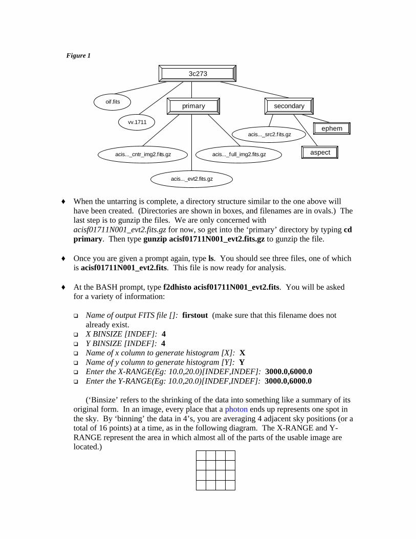
♦ When the untarring is complete, a directory structure similar to the one above willhave been created. (Directories are shown in boxes, and filenames are in ovals.) Thelast step is to gunzip the files. We are only concerned withacisf01711N001_evt2.fits.gz for now, so get into the ‘primary’ directory by typing cdprimary. Then type gunzip acisf01711N001_evt2.fits.gz to gunzip the file.

♦ Once you are given a prompt again, type ls. You should see three files, one of whichis acisf01711N001_evt2.fits. This file is now ready for analysis.

♦ At the BASH prompt, type f2dhisto acisf01711N001_evt2.fits. You will be askedfor a variety of information:

q Name of output FITS file []: firstout (make sure that this filename does notalready exist.

q X BINSIZE [INDEF]: 4q Y BINSIZE [INDEF]: 4q Name of x column to generate histogram [X]: Xq Name of y column to generate histogram [Y]: Yq Enter the X-RANGE(Eg: 10.0,20.0)[INDEF,INDEF]: 3000.0,6000.0q Enter the Y-RANGE(Eg: 10.0,20.0)[INDEF,INDEF]: 3000.0,6000.0

(‘Binsize’ refers to the shrinking of the data into something like a summary of itsoriginal form. In an image, every place that a photon ends up represents one spot inthe sky. By ‘binning’ the data in 4’s, you are averaging 4 adjacent sky positions (or atotal of 16 points) at a time, as in the following diagram. The X-RANGE and Y-RANGE represent the area in which almost all of the parts of the usable image arelocated.)

3c273

primary secondary

aspect

ephem

oif .fits

vv.1711

acis..._cntr_img2.f its.gz acis..._full_img2.fits.gz

acis..._evt2.fits.gz

acis..._src2.f its.gz

Figure 1

♦ FTOOLS will state a summary of what you entered and then return the BASHprompt. At this point, find the Fv icon on your desktop (shown below) and double-click on it.

♦ Multiple windows will open. Find the one labeled ‘fv: File Dialog’. You’ll see a listof files and directories under ‘Contents’: you want to find the output file you justcreated, firstout. Double-click on 3c273/, then on primary/. You should then seefour filenames, one of which is firstout. Click on firstout, and then click on the‘Open’ button.

♦ Another window will pop up, labeled ‘fv: Summary of firstout inC:/ftools/3c273/primary’. Click on the ‘Image’ button under the ‘View’ heading.(Note: You may get an error message saying that Fv is unable to find a file. If thishappens, exit Fv (close ALL of its windows) and then reopen Fv by double-clicking onthe icon.)

♦ A window will open that contains a grid on which your image is displayed. Move thewindow so that it is as close to the top of your screen as possible. Then, using thezoom button, zoom in twice. You’ll see the blue box around the picture in the upperright hand corner get smaller. Click on the blue box and drag it so that it is centeredon the image. (The image should look something like a small blob right now.) Oncethe image is in the center of the blue box, zoom in two more times.

♦ Using the scroll-bar on the right side of the grid, scroll so that you can see the entireimage. Place the cursor (without clicking) on the center of the circular part of theimage. Look at the box in the upper left hand corner, labeled ‘Image Pixel’. It shouldcontain numbers close to ( 278, 236 ). Copy down these numbers on a piece of paperand then close all of the Fv windows.

♦ Back in your BASH terminal, type f2dhisto <filename>, and again replace<filename> with acisf01711N001_evt2.fits.

♦ You will be prompted for the same information as before, except this time youranswers will be slightly different:

q Name of output FITS file[firstout]: output2 (Again, make sure that this file namedoesn’t already exist.)

q X BINSIZE [4]: 1q Y BINSIZE [4]: 1q Name of x column to generate histogram [X]: Xq Name of y column to generate histogram [Y]: Y

♦ X-RANGE and Y-RANGE: For this information, you need to do some calculations.For the X-RANGE, you must first correct for the binsize of 4 from earlier. To dothis, multiple the X value from your ‘Image Pixel’ coordinates (~278) by 4. Add thisnumber to your initial starting value for X, 3000. This should give you a numbersimilar to 4112. Your X-RANGE needs to encompass about 100 on either side of thisnumber. Thus, enter 4000.0,4200.0 for the X-RANGE.

For the Y-RANGE, follow the same process. Multiply the Y value from your‘Image Pixel’ coordinates (~236) by 4 and then add this to your initial starting valuefor Y, 3000. This should give you a number close to 3944. Therefore, enter3850.0,4050.0 for your Y-RANGE.

♦ FTOOLS will summarize the information it will be entering into f2dhisto, and thenreturn the BASH prompt. Now, find the Fv icon on your desktop and double-click onit to begin Fv.

♦ In the ‘File Dialog’ window, find output2, select it and click the ‘Open’ button.(Hint: Follow the path 3c273/primary/output2.)

♦ Another window will pop up, labeled ‘fv: Summary of output2 inC:/ftools/3c273/primary’. Like before, click on the ‘Image’ button under the ‘View’heading.

♦ A window will open which contains your image of 3c273 on a grid. Move thewindow as close to the top of your screen as possible and use the scroll bar on theright hand side to scroll so that you can view the entire image. Use the ‘Zoom In’button to zoom in twice. Move the blue box in the upper right hand corner so that itis centered on the circular part of the source. (The other part of the image is a jet.We will be analyzing that part later.)

♦ In the upper left hand corner of the window, there are four menu headings. Click on‘Edit’ and then select ‘Region Files’. A window labeled ‘Edit Region’ will open.Select ‘Pixels’ underneath the scroll bar.

♦ Next, go back to the window containing your image. Right click on the center of themain source and, holding the mouse button down, pull the cursor away from thecenter. This will drag a circle around the source. Make the circle big enough toencompass the entire main source, and then release the mouse button. Clicking andholding the left mouse button anywhere inside the circle allows you to then move thecircle if you wish.

♦ Return to the ‘Edit Region’ box. Copy onto a piece of paper the numbers that you seethere. (They will look something like Circle(109.05, 91.8499, 13.3185).) You willbe using these in the next step. Once you have recorded these values, you can closeall of the Fv windows and return to your BASH terminal.

♦ At the prompt, type fselect. You will be asked for the following information:q Name of FITS file and [ext#][]: acisf01711N001_evt2.fitsq Name of output FITS file[]: region1.fits

♦ Selection Expression[]: This is where you will use the numbers you copied downfrom the ‘Edit Region’ box. First, add the starting X value that you entered into thelast f2dhisto method (4000), to the first number in the Circle expression from the‘Edit Region’ box (~109.05). Next, add the starting Y value that you entered intof2dhisto (3850) to the second number in the Circle expression (~91.8499). Recordthese two values on a piece of paper.

♦ Enter these values for the Selection Expression[] EXACTLY as follows: (The onlydifference might be the actual values, which may differ by a small amount.)“circle(4109.05,3941.8499,13.3185,x,y)”

♦ At the next prompt, type fhisto region1.fits 3c273_lcurve.fits time 100 (Thisrepresents the input file, the output file, the keyword and the binsize in seconds,respectively.) FTOOLS will repeat the information you just entered, and then returna prompt. Go back to your desktop, and open Fv.

♦ Find the file you just created, 3c273_lcurve.fits (using the path3c273/primary/3c273_lcurve.fits), select it and click on the ‘Open’ button.

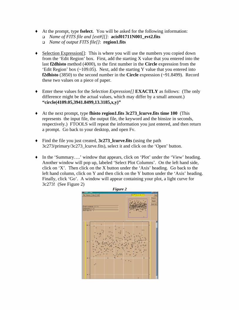
♦ In the ‘Summary….’ window that appears, click on ‘Plot’ under the ‘View’ heading.Another window will pop up, labeled ‘Select Plot Columns’. On the left hand side,click on ‘X’. Then click on the X button under the ‘Axis’ heading. Go back to theleft hand column, click on Y and then click on the Y button under the ‘Axis’ heading.Finally, click ‘Go’. A window will appear containing your plot, a light curve for3c273! (See Figure 2)

Figure 2

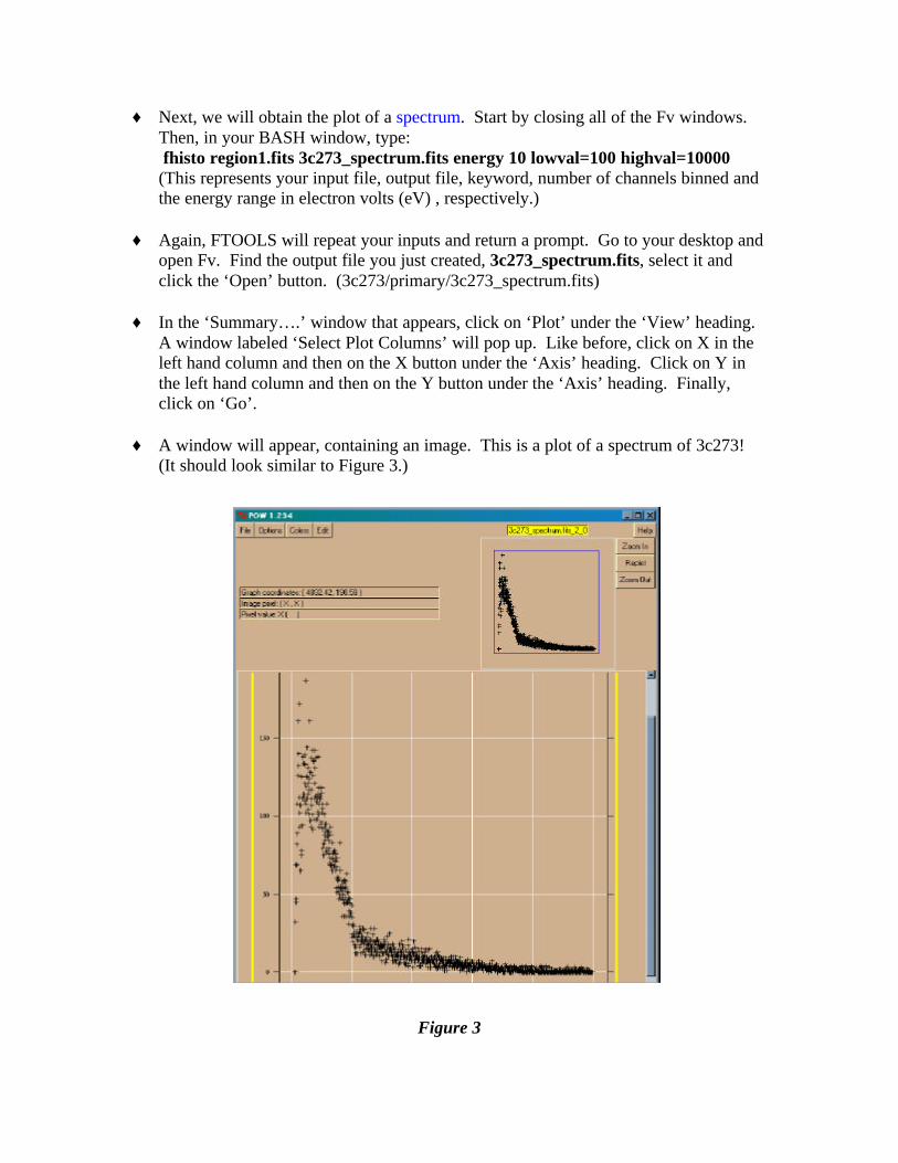
♦ Next, we will obtain the plot of a spectrum. Start by closing all of the Fv windows.Then, in your BASH window, type: fhisto region1.fits 3c273_spectrum.fits energy 10 lowval=100 highval=10000(This represents your input file, output file, keyword, number of channels binned andthe energy range in electron volts (eV) , respectively.)

♦ Again, FTOOLS will repeat your inputs and return a prompt. Go to your desktop andopen Fv. Find the output file you just created, 3c273_spectrum.fits, select it andclick the ‘Open’ button. (3c273/primary/3c273_spectrum.fits)

♦ In the ‘Summary….’ window that appears, click on ‘Plot’ under the ‘View’ heading.A window labeled ‘Select Plot Columns’ will pop up. Like before, click on X in theleft hand column and then on the X button under the ‘Axis’ heading. Click on Y inthe left hand column and then on the Y button under the ‘Axis’ heading. Finally,click on ‘Go’.

♦ A window will appear, containing an image. This is a plot of a spectrum of 3c273!(It should look similar to Figure 3.)

Figure 3

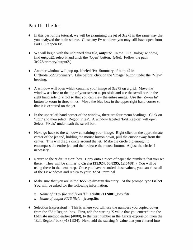
Part II: The Jet

♦ In this part of the tutorial, we will be examining the jet of 3c273 in the same way thatyou analyzed the main source. Close any Fv windows you may still have open fromPart I. Reopen Fv.

♦ We will begin with the unbinned data file, output2. In the ‘File Dialog’ window,find output2, select it and click the ‘Open’ button. (Hint: Follow the path3c273/primary/output2.)

♦ Another window will pop up, labeled ‘fv: Summary of output2 inC:/ftools/3c273/primary’. Like before, click on the ‘Image’ button under the ‘View’heading.

♦ A window will open which contains your image of 3c273 on a grid. Move thewindow as close to the top of your screen as possible and use the scroll bar on theright hand side to scroll so that you can view the entire image. Use the ‘Zoom In’button to zoom in three times. Move the blue box in the upper right hand corner sothat it is centered on the jet.


♦ Next, go back to the window containing your image. Right click on the approximatecenter of the jet and, holding the mouse button down, pull the cursor away from thecenter. This will drag a circle around the jet. Make the circle big enough toencompass the entire jet, and then release the mouse button. Adjust the circle ifnecessary.

♦ Return to the ‘Edit Region’ box. Copy onto a piece of paper the numbers that you seethere. (They will be similar to Circle(131.924, 66.8295, 12.5408).) You will beusing these in the next step. Once you have recorded these values, you can close allof the Fv windows and return to your BASH terminal.

♦ Make sure that you are in the 3c273/primary/ directory. At the prompt, type fselect.You will be asked for the following information:

q Name of FITS file and [ext#][]: acisf01711N001_evt2.fitsq Name of output FITS file[]: jetreg.fits

♦ Selection Expression[]: This is where you will use the numbers you copied downfrom the ‘Edit Region’ box. First, add the starting X value that you entered into thef2dhisto method earlier (4000), to the first number in the Circle expression from the‘Edit Region’ box (~131.924). Next, add the starting Y value that you entered into

f2dhisto (3850) to the second number in the Circle expression (~66.8295). Recordthese two values on a piece of paper.


♦ At the next prompt, type fhisto jetreg.fits 3c273_jet_lcurve.fits time 100 (Thisrepresents the input file, the output file, the keyword and the binsize in seconds,respectively.) FTOOLS will repeat the information you just entered, and then returna prompt. Go back to your desktop, and open Fv.

♦ Find the file you just created, 3c273_jet_lcurve.fits (using the path3c273/primary/3c273_jet_lcurve.fits), select it and click on the ‘Open’ button.

♦ In the ‘Summary….’ window that appears, click on ‘Plot’ under the ‘View’ heading.

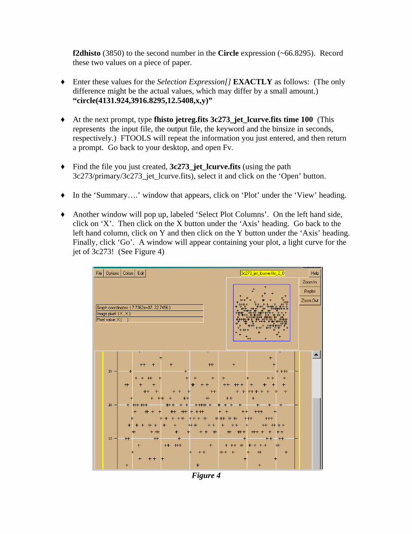
♦ Another window will pop up, labeled ‘Select Plot Columns’. On the left hand side,click on ‘X’. Then click on the X button under the ‘Axis’ heading. Go back to theleft hand column, click on Y and then click on the Y button under the ‘Axis’ heading.Finally, click ‘Go’. A window will appear containing your plot, a light curve for thejet of 3c273! (See Figure 4)

Figure 4

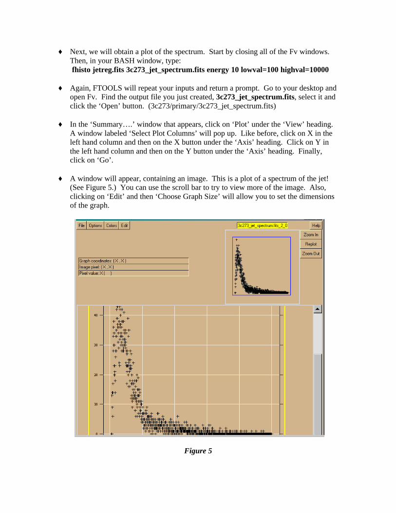
♦ Next, we will obtain a plot of the spectrum. Start by closing all of the Fv windows.Then, in your BASH window, type: fhisto jetreg.fits 3c273_jet_spectrum.fits energy 10 lowval=100 highval=10000

♦ Again, FTOOLS will repeat your inputs and return a prompt. Go to your desktop andopen Fv. Find the output file you just created, 3c273_jet_spectrum.fits, select it andclick the ‘Open’ button. (3c273/primary/3c273_jet_spectrum.fits)


♦ A window will appear, containing an image. This is a plot of a spectrum of the jet!(See Figure 5.) You can use the scroll bar to try to view more of the image. Also,clicking on ‘Edit’ and then ‘Choose Graph Size’ will allow you to set the dimensionsof the graph.

Figure 5

Part III: Cassiopeia A

Cassiopeia A (Cas A) is a 320-year-old supernova remnant. Amassive star exploded, ejecting a shell of matter that created abubble of gas 10 light years in diameter with a temperature ofabout 50 million degrees. As this hot gas expands, (and it willcontinue to do so for thousands of years), it produces x-rays.Astronomers can use this data to find x-ray spectra and thenuse these spectra to determine the chemical makeup of Cas A.The image to the right was made with the Advanced CCDImaging Spectrometer (ACIS) over the span of 5,000 seconds. The outer shock wave canbe compared to a sonic boom. (Check out http://chandra.harvard.edu/press/casfact.htmlfor more about supernovae and Cas A.)

♦ Begin by closing all of the Fv windows you have open from the previous sections. Inyour BASH window, type cd /ftools to get back to your main directory. Create afolder for your Cas A data by typing mkdir cas_a.

♦ Open Netscape and go to http://asc.harvard.edu.

♦ At the top of the page, you’ll see various buttons: click on the one that says Archive.

♦ A page will open that says “Welcome to the Chandra Data Archive”. You’ll see a listof links: click on Search and Retrieve.

♦ The next page will be “Search and Retrieval from the Chandra Data Archive”. If youscroll down the page a bit, you will see Provisional Web Interface for Browsingand Retrieval in blue. Click on this link.

♦ You have now entered the Chandra Data Archive. Scroll down to “View InformationAbout Public Observations Available for Retrieval from the Archive…”. Below thisheading there will be four buttons. Click on Sort by RA & Dec.

♦ Upon scrolling down the next page, you’ll see a long table of observations. Find theobservation whose ObsId is 1512, whose Object Name is CAS A, CHIP S2 andwhose RA (right ascension) is 23:22:46. Click on 1512.

♦ You’ll then be returned to the Chandra Data Archive page that you were at earlier.This time, however, if you scroll down, you’ll see that 1512 has been entered into theEnter ObsId box. Scroll down a little bit more and make sure that the fullyprocessed science products box is checked, inside the Product Categories box.Click on Browse Archive and Retrieve Data Products.

♦ You will receive a list of four files. Upon scrolling down further, you’ll see theinstructions “Select files to retrieve from archive”. In the white box below, click onthe first file, hold down the shift key, and then click on the fourth file. This willallow you to select all four files. With all four files selected, click on RETRIEVEfrom Archive.

♦ The next page will give you the name of your tar file. After copying this filenamedown for future reference, find the sentence that says “Or you may download itdirectly here”. Click on here.

♦ A window will appear which asks you whether you’d like to save the file to disk oropen it. Select Save to disk and then click OK.

♦ Next, a window entitled “Save As…” will open. In the File name: field, the name ofyour tar file will already be entered. In the Save in: field, make sure that you aresaving the tar file into your cas_a folder. Once this is done, click Save.

♦ Minimize Netscape and return to your BASH window.

♦ At the prompt, use the commands you know to make your way to the cas_a directory.Once you are in this directory, type ls to view its contents. You will see the file youdownloaded. (It should look something like retrieve_1512_7166.tar, but the last fournumbers may be different.)

♦ Type tar xvf <filename.tar>, replacing <filename.tar> with the name of the file youdownloaded. This will untar the data and save it into the directory cas_a.

♦ When the untarring is complete, a directory structure similar to the one set up for3c273 will be created. The last step is to gunzip the files. We are only concernedwith acisf01512N001_evt2.fits.gz for now, so enter the primary/ directory by typingcd primary. Then type gunzip acisf01512N001_evt2.fits.gz to gunzip the file.

♦ Once you are given a prompt again, type ls. You should see three files, one of whichis acisf01711N001_evt2.fits. This file is now ready for analysis.

♦ At the BASH prompt, type f2dhisto acisf01512N001_evt2.fits. You will be askedfor a variety of information:

q Name of output FITS file []: casfirstout (make sure that this filename does notalready exist.

q X BINSIZE [INDEF]: 4q Y BINSIZE [INDEF]: 4q Name of x column to generate histogram [X]: Xq Name of y column to generate histogram [Y]: Yq Enter the X-RANGE(Eg: 10.0,20.0)[INDEF,INDEF]: 3000.0,6000.0q Enter the Y-RANGE(Eg: 10.0,20.0)[INDEF,INDEF]: 3000.0,6000.0

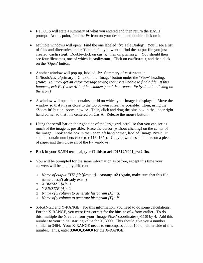
♦ FTOOLS will state a summary of what you entered and then return the BASHprompt. At this point, find the Fv icon on your desktop and double-click on it.

♦ Multiple windows will open. Find the one labeled ‘fv: File Dialog’. You’ll see a listof files and directories under ‘Contents’: you want to find the output file you justcreated, casfirstout. Double-click on cas_a/, then on primary/. You should thensee four filenames, one of which is casfirstout. Click on casfirstout, and then clickon the ‘Open’ button.

♦ Another window will pop up, labeled ‘fv: Summary of casfirstout inC:/ftools/cas_a/primary’. Click on the ‘Image’ button under the ‘View’ heading.(Note: You may get an error message saying that Fv is unable to find a file. If thishappens, exit Fv (close ALL of its windows) and then reopen Fv by double-clicking onthe icon.)

♦ A window will open that contains a grid on which your image is displayed. Move thewindow so that it is as close to the top of your screen as possible. Then, using the‘Zoom In’ button, zoom in twice. Then, click and drag the blue box in the upper righthand corner so that it is centered on Cas A. Release the mouse button.

♦ Using the scroll-bar on the right side of the large grid, scroll so that you can see asmuch of the image as possible. Place the cursor (without clicking) on the center ofthe image. Look at the box in the upper left hand corner, labeled ‘Image Pixel’. Itshould contain numbers close to ( 116, 167 ). Copy down these numbers on a pieceof paper and then close all of the Fv windows.

♦ Back in your BASH terminal, type f2dhisto acisf01512N001_evt2.fits.

♦ You will be prompted for the same information as before, except this time youranswers will be slightly different:

q Name of output FITS file[firstout]: casoutput2 (Again, make sure that this filename doesn’t already exist.)

q X BINSIZE [4]: 1q Y BINSIZE [4]: 1q Name of x column to generate histogram [X]: Xq Name of y column to generate histogram [Y]: Y

♦ X-RANGE and Y-RANGE: For this information, you need to do some calculations.For the X-RANGE, you must first correct for the binsize of 4 from earlier. To dothis, multiple the X value from your ‘Image Pixel’ coordinates (~116) by 4. Add thisnumber to your initial starting value for X, 3000. This should give you a numbersimilar to 3464. Your X-RANGE needs to encompass about 100 on either side of thisnumber. Thus, enter 3360.0,3560.0 for the X-RANGE.

For the Y-RANGE, follow the same process. Multiply the Y value from your‘Image Pixel’ coordinates (~167) by 4 and then add this to your initial starting valuefor Y, 3000. This should give you a number close to 3668. Therefore, enter3560.0,3760.0 for your Y-RANGE.

♦ FTOOLS will summarize the information it will be entering into f2dhisto, and thenreturn the BASH prompt. Now, find the Fv icon on your desktop and double-click onit to begin Fv.

♦ In the ‘File Dialog’ window, find casoutput2, select it and click the ‘Open’ button.(Hint: Follow the path cas_a/primary/casoutput2.)

♦ Another window will pop up, labeled ‘fv: Summary of casoutput2 inC:/ftools/cas_a/primary’. Like before, click on the ‘Image’ button under the ‘View’heading.

♦ A window will open which contains your image of Cas A on a grid. However, theimage is too big! To fit the entire image on the grid, you need to go back and try adifferent X-RANGE and Y-RANGE. Close all Fv windows and return to your BASHwindow. Again, type f2dhisto acisf01512N001_evt2.fits at the prompt. This time,enter casout for the output filename, 1 for each binsize, X and Y for the columnnames; finally, try 3100.0,3800.0 for the X-RANGE and 3250.0,3950.0 for the Y-RANGE.

♦ Once a prompt is returned, find the Fv icon on your desktop and double-click on it toopen Fv.

♦ In the ‘File Dialog’ window, find casout, select it and click the ‘Open’ button.

♦ Another window will pop up, labeled ‘fv: Summary of casout inC:/ftools/cas_a/primary’. Like before, click on the ‘Image’ button under the ‘View’heading.

♦ This time when the grid opens, you should see that the image just about fits on thegrid. This is sufficient, but you can go back and make the grid slightly larger if youwish.


♦ Next, go back to the window containing your image. Right click on the center of theimage and, holding the mouse button down, pull the cursor away from the center.This will drag a circle around Cas A. Make the circle big enough to encompass the

entire supernova, and then release the mouse button. Clicking and holding the leftmouse button anywhere inside the circle allows you to then move the circle if youwish.

♦ Return to the ‘Edit Region’ box. Copy onto a piece of paper the numbers that you seethere. (They will look something like Circle(370.1, 419.1, 309.176).) You will beusing these in the next step. Once you have recorded these values, you can close allof the Fv windows and return to your BASH terminal.

♦ At the prompt, type fselect. You will be asked for the following information:

q Name of FITS file and [ext#][]: acisf01512N001_evt2.fitsq Name of output FITS file[]: cas_a_reg.fits

♦ Selection Expression[]: This is where you will use the numbers you copied downfrom the ‘Edit Region’ box. First, add the starting X value that you entered into thelast f2dhisto method (3100), to the first number in the Circle expression from the‘Edit Region’ box (~370.1). Next, add the starting Y value that you entered intof2dhisto (3250) to the second number in the Circle expression (~419.1). Recordthese two values on a piece of paper.


♦ When a prompt is returned (Note: processing the last step may take awhile), typefhisto cas_a_reg.fits cas_a_lcurve.fits expno 1 (The first two parts are the input fileand output file, respectively. The third piece of information, the keyword expno, isthe exposure number for the observation. Finally, the last part, 1, is the binsize.Specifically, 1 indicates that every exposure interval is plotted separately.) FTOOLSwill repeat the information you just entered, and then return a prompt. Go back toyour desktop, and open Fv.

♦ Find the file you just created, cas_a_lcurve.fits (using the pathcas_a/primary/cas_a_lcurve.fits), select it and click on the ‘Open’ button.

♦ In the ‘Summary….’ window that appears, click on ‘Plot’ under the ‘View’ heading.Another window will pop up, labeled ‘Select Plot Columns’. On the left hand side,click on ‘X’. Then click on the X button under the ‘Axis’ heading. Go back to theleft hand column, click on Y and then click on the Y button under ‘Axis’. Finally,click ‘Go’. A window will appear containing a plot of a light curve for Cas A! (Itshould look similar to Figure 6.)

Figure 6

♦ Next, we will obtain a plot of the spectrum. Start by closing all of the Fv windows.Then, in your BASH window, type: fhisto cas_a_reg.fits cas_a_spectrum.fits energy 10 lowval=100 highval=10000

♦ Again, FTOOLS will repeat your inputs and return a prompt. Go to your desktop andopen Fv. Find the output file you just created, cas_a_spectrum.fits, select it andclick the ‘Open’ button. (cas_a/primary/cas_a_spectrum.fits)


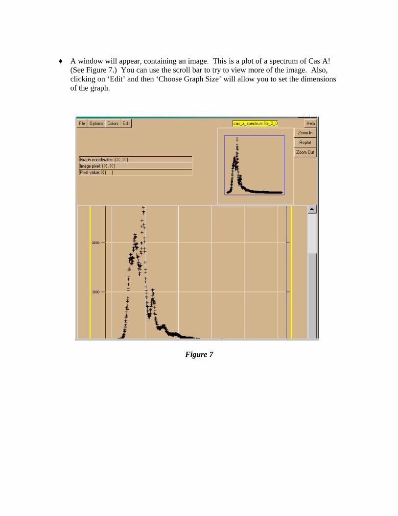
♦ A window will appear, containing an image. This is a plot of a spectrum of Cas A!(See Figure 7.) You can use the scroll bar to try to view more of the image. Also,clicking on ‘Edit’ and then ‘Choose Graph Size’ will allow you to set the dimensionsof the graph.

Figure 7

using ftools and fv for data analysis: chandramatilsky/documents/windows/tutorial4.pdf · using...

Documents