using derivative analysis to improve pumping test ...ky.aipg.org/pdf/glenn...
TRANSCRIPT
© 2014 HydroSOLVE, Inc.
Using Derivative Analysis to Improve Pumping Test Interpretation with the Cooper and Jacob Method
Glenn M. Duffield
HydroSOLVE, Inc.
703.264.9024
www.aqtesolv.com

© 2014 HydroSOLVE, Inc.
What Is a Pumping Test?
An aquifer test performed with a controlled pumping rate
– constant-rate test
– step-drawdown test (well performance)
– recovery test
Water-level response (drawdown) measured in control well and one or more observation wells
© 2014 HydroSOLVE, Inc.
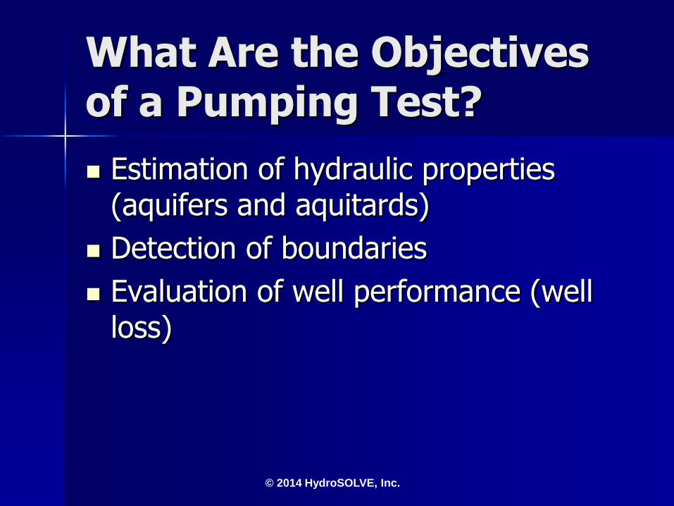
What Are the Objectives of a Pumping Test?
Estimation of hydraulic properties (aquifers and aquitards)
Detection of boundaries
Evaluation of well performance (well loss)
© 2014 HydroSOLVE, Inc.
Analysis of Pumping Test Data
Traditional Methods

© 2014 HydroSOLVE, Inc.
Theis (1935) introduced a type-curve matching technique for estimating aquifer properties from a constant-rate pumping test assuming a fully penetrating pumping well in a homogeneous and isotropic nonleaky confined aquifer of infinite extent and constant thickness…
In The Beginning…
there was Theis!

© 2014 HydroSOLVE, Inc.
In The Beginning… there was Theis!
100
101
102
10310
-2
10-1
100
101
1/u
w(u
)
100
101
102
10310
-1
100
101
102
Time (min)
Dra
wd
ow
n (
ft)
)(
4uw
s
QT
2
4
r
uTtS
s*, t*, w(u)*, u*

© 2014 HydroSOLVE, Inc.
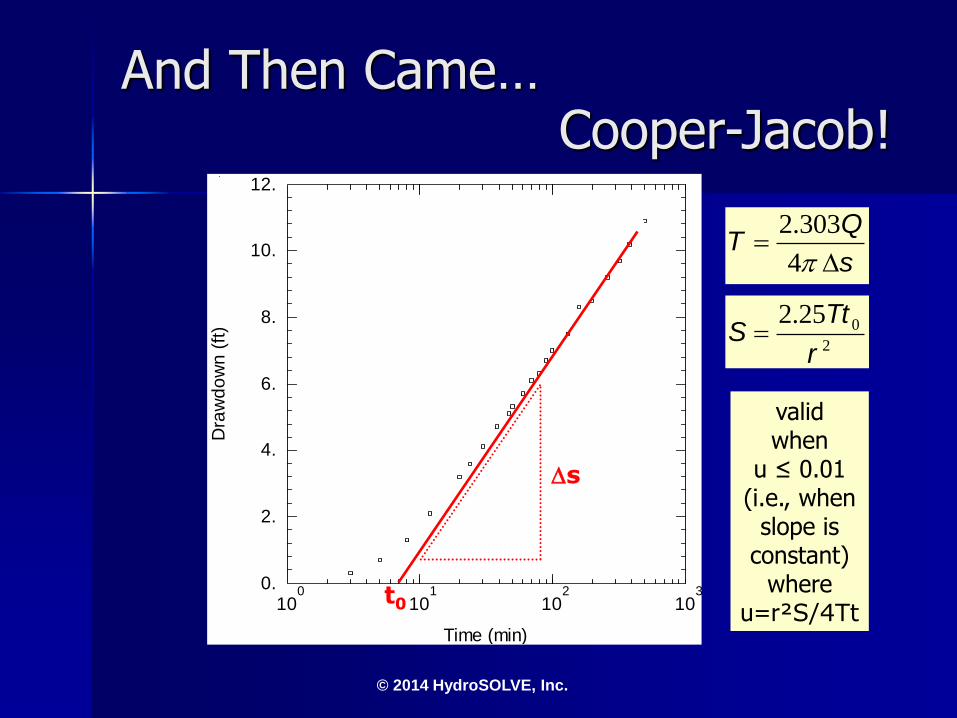
Cooper and Jacob (1946) subsequently discovered that the Theis solution, drawn on semilog axes, plots as a straight line after sufficiently long periods of pumping…
And Then Came…
Cooper and Jacob!
© 2014 HydroSOLVE, Inc.
And Then Came… Cooper-Jacob!
100
101
102
1030.
2.
4.
6.
8.
10.
12.
Time (min)
Dra
wd
ow
n (
ft)
2
025.2
r
TtS
s
QT
4
303.2
t0
s
valid when
u ≤ 0.01 (i.e., when
slope is constant)
where u=r²S/4Tt

© 2014 HydroSOLVE, Inc.
Pumping Test Data Analysis
How often is the Cooper and Jacob method the first step in your analysis of pumping test data?
Are there techniques you could use to get more reliable results?
© 2014 HydroSOLVE, Inc.
A Different Approach...
A more productive approach to pumping test data analysis begins with the application of derivative analysis that helps you to:
– identify common flow regimes
– guide subsequent curve matching
What is derivative analysis?

© 2014 HydroSOLVE, Inc.
Derivative Analysis
Technique popularized in the petroleum industry (Bourdet et al. 1983)
Plot of ∂s/∂lnt vs t
Derivatives are calculated from field data
A derivative plot, which combines the display of drawdown and derivative data, is a powerful diagnostic and curve matching tool

© 2014 HydroSOLVE, Inc.
Interpretation of Derivative slope of drawdown data on semilog plot
10-1
100
101
102
103
1040.
2.
4.
6.
8.
10.
Dimensionless Time
Dim
en
sio
nle
ss
Dra
wd
ow
nTheis drawdown
solution derivative is
constant at
late time when
Cooper and
Jacob solution
is valid
(infinite-acting
radial flow
regime)
IARF (plateau)

© 2014 HydroSOLVE, Inc.
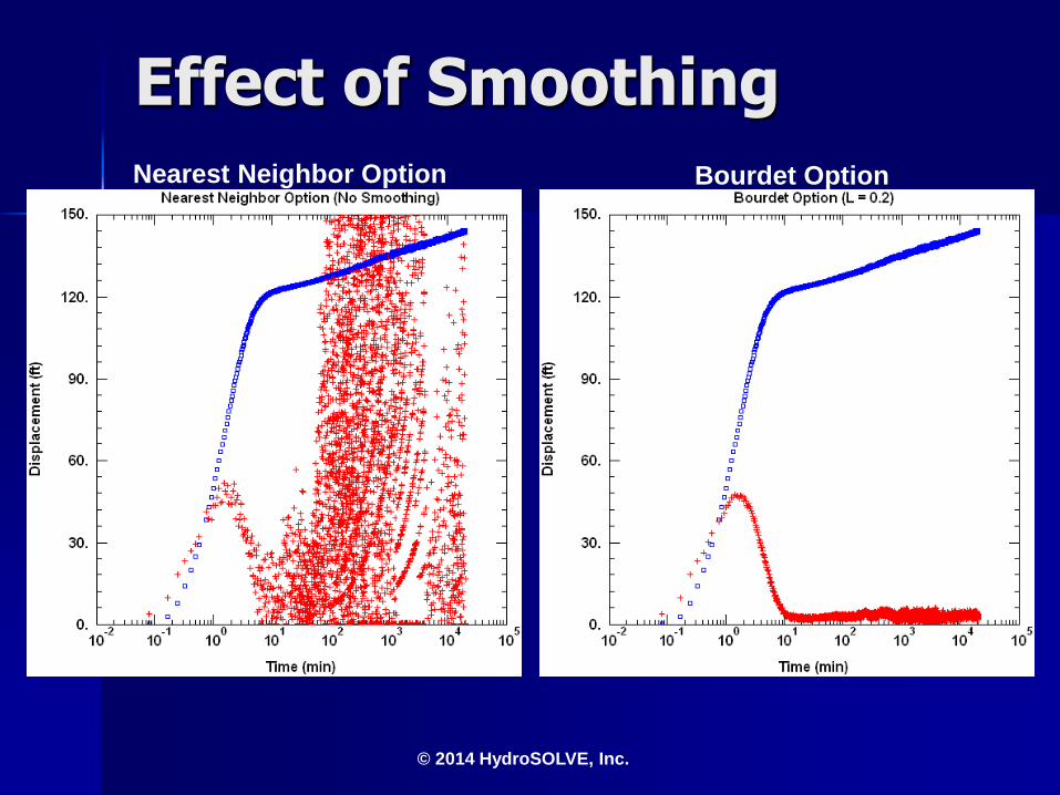
Derivative Smoothing
Derivatives computed directly from field data are often noisy
Four smoothing options are available in AQTESOLV to reduce noise
– nearest neighbor (no smoothing)
– Bourdet method
– Spane method
– smoothing
Begin with
nearest
neighbor method.
Avoid excessive
smoothing!
© 2014 HydroSOLVE, Inc.
Effect of Smoothing Nearest Neighbor Option Bourdet Option
© 2014 HydroSOLVE, Inc.
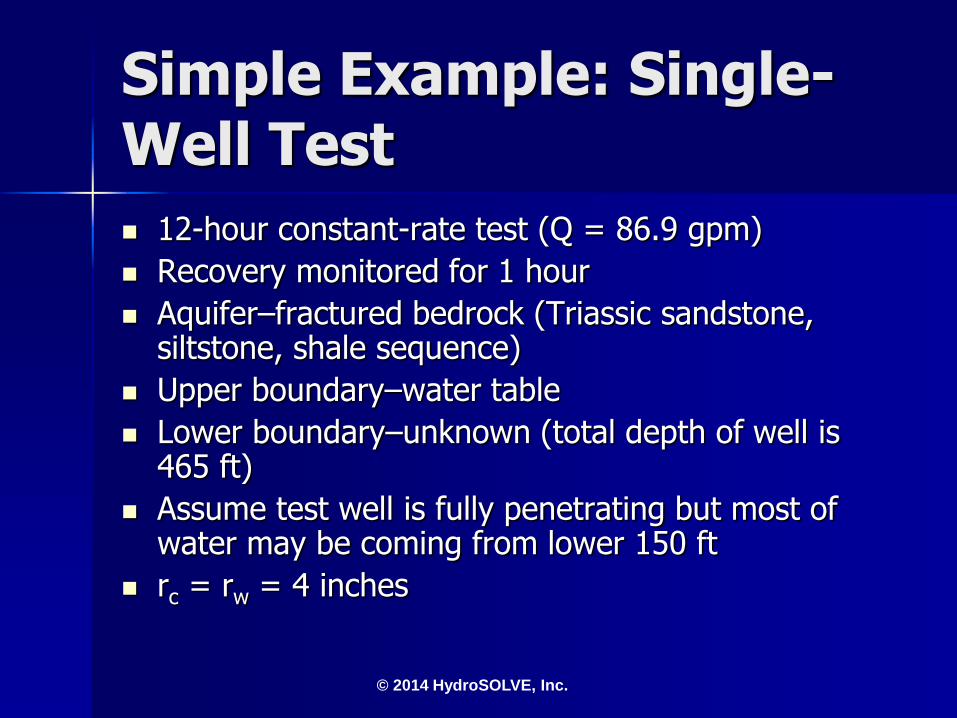
Simple Example: Single-Well Test
12-hour constant-rate test (Q = 86.9 gpm)
Recovery monitored for 1 hour
Aquifer–fractured bedrock (Triassic sandstone, siltstone, shale sequence)
Upper boundary–water table
Lower boundary–unknown (total depth of well is 465 ft)
Assume test well is fully penetrating but most of water may be coming from lower 150 ft
rc = rw = 4 inches
© 2014 HydroSOLVE, Inc.
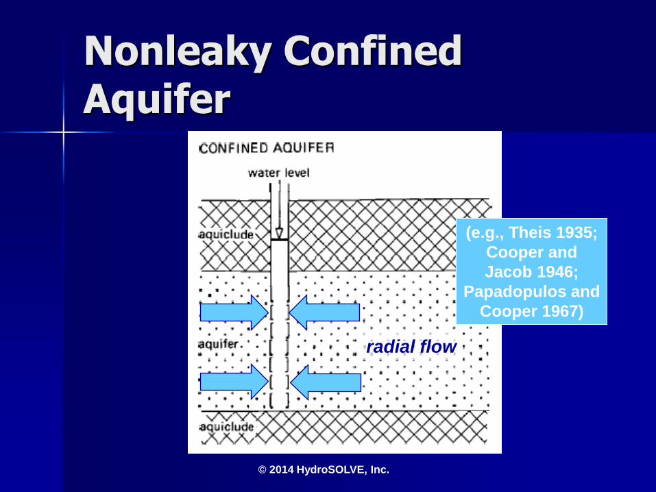
Nonleaky Confined Aquifer
(e.g., Theis 1935;
Cooper and
Jacob 1946;
Papadopulos and
Cooper 1967)
radial flow
© 2014 HydroSOLVE, Inc.
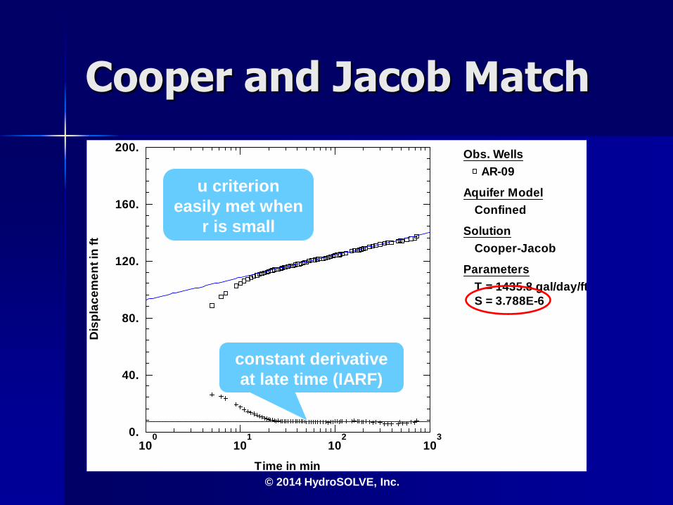
Cooper and Jacob Match
100
101
102
1030.
40.
80.
120.
160.
200.
Time in min
Dis
pla
ce
me
nt
in f
t
Obs. Wells
AR-09
Aquifer Model
Confined
Solution
Cooper-Jacob
Parameters
T = 1435.8 gal/day/ft
S = 3.788E-6
u criterion
easily met when
r is small
constant derivative
at late time (IARF)
© 2014 HydroSOLVE, Inc.
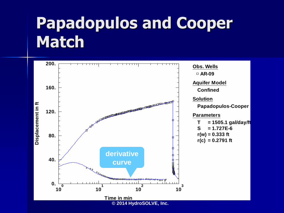
Papadopulos and Cooper Match
100
101
102
1030.
40.
80.
120.
160.
200.
Time in min
Dis
pla
ce
me
nt
in f
t
Obs. Wells
AR-09
Aquifer Model
Confined
Solution
Papadopulos-Cooper
Parameters
T = 1505.1 gal/day/ft
S = 1.727E-6
r(w) = 0.333 ft
r(c) = 0.2791 ft
derivative
curve

© 2014 HydroSOLVE, Inc.
Key Concepts and Tips
Combine derivative analysis with the Cooper and Jacob method to
– identify IARF period (derivative plateau)
– improve fitting of straight line
Cooper and Jacob can obtain results comparable with more rigorous methods with less effort

© 2014 HydroSOLVE, Inc.
Key Concepts and Tips
Cooper and Jacob applied to single-well tests can yield reliable estimates of T; however, S often will be biased due to partial penetration and/or well losses.

© 2014 HydroSOLVE, Inc.
Case Study: Coastal Aquifer Oude Korendijk, The Netherlands
14-hour constant-rate test (Q = 788 m3/day)
Aquifer–7 m of coarse sand with some gravel
Upper boundary–18 m of clay, peat and clayey fine sand; note clayey fine sand directly above aquifer
Lower boundary–fine sand and clay sediments
Test well is fully penetrating
Observation wells at r = 30, 90 and 215 m from pumped well
Source: Kruseman and de Ridder (1994)

© 2014 HydroSOLVE, Inc.
Stratigraphy
from Kruseman and de Ridder (1994)

© 2014 HydroSOLVE, Inc.
Cooper and Jacob Analysis
Kruseman and de Ridder assumed a nonleaky confined aquifer for the analysis of the constant-rate pumping test.
Let’s consider interpretations of drawdown data with and without derivative analysis…
© 2014 HydroSOLVE, Inc.
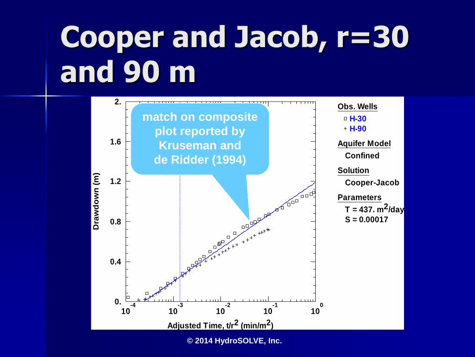
Cooper and Jacob, r=30 and 90 m
10-4
10-3
10-2
10-1
1000.
0.4
0.8
1.2
1.6
2.
Adjusted Time, t/r2 (min/m2)
Dra
wd
ow
n (
m)
Obs. Wells
H-30
H-90
Aquifer Model
Confined
Solution
Cooper-Jacob
Parameters
T = 437. m2/day
S = 0.00017
match on composite
plot reported by
Kruseman and
de Ridder (1994)
© 2014 HydroSOLVE, Inc.
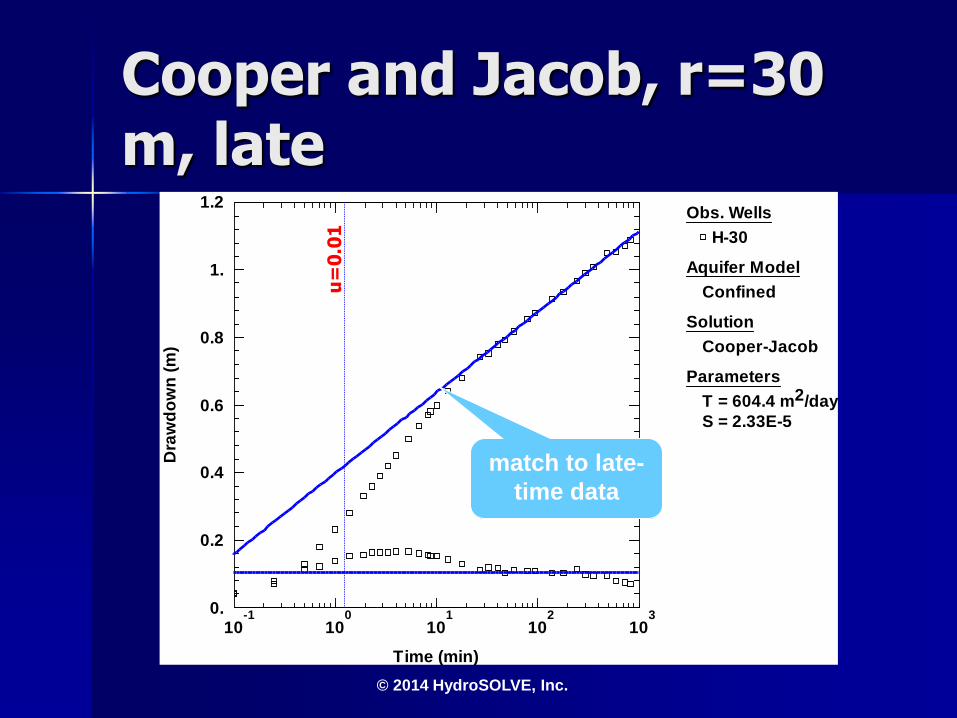
Cooper and Jacob, r=30 m, late
10-1
100
101
102
1030.
0.2
0.4
0.6
0.8
1.
1.2
Time (min)
Dra
wd
ow
n (
m)
Obs. Wells
H-30
Aquifer Model
Confined
Solution
Cooper-Jacob
Parameters
T = 604.4 m2/day
S = 2.33E-5
u=
0.0
1
match to late-
time data

© 2014 HydroSOLVE, Inc.
Cooper and Jacob, r=30 m, early
10-1
100
101
102
1030.
0.2
0.4
0.6
0.8
1.
1.2
Time (min)
Dra
wd
ow
n (
m)
Obs. Wells
H-30
Aquifer Model
Confined
Solution
Cooper-Jacob
Parameters
T = 376.3 m2/day
S = 0.0001744
u=
0.1
match to early-
time data
© 2014 HydroSOLVE, Inc.
Cooper and Jacob Results
We have three very different estimates of T and S. Which interpretation is most reliable?
Let’s consider the response of a leaky confined aquifer with aquitard storage and its associated derivative plot…

© 2014 HydroSOLVE, Inc.
Leaky Confined Aquifer
(e.g., Hantush
and Jacob 1955;
Hantush 1960)
radial flow
© 2014 HydroSOLVE, Inc.
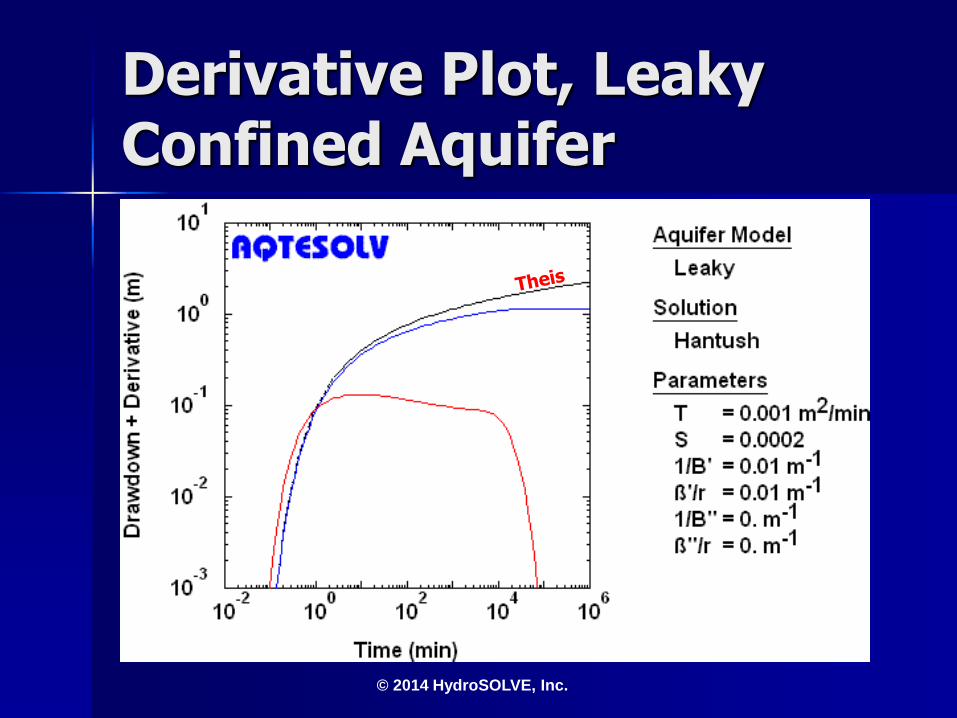
Derivative Plot, Leaky Confined Aquifer
© 2014 HydroSOLVE, Inc.
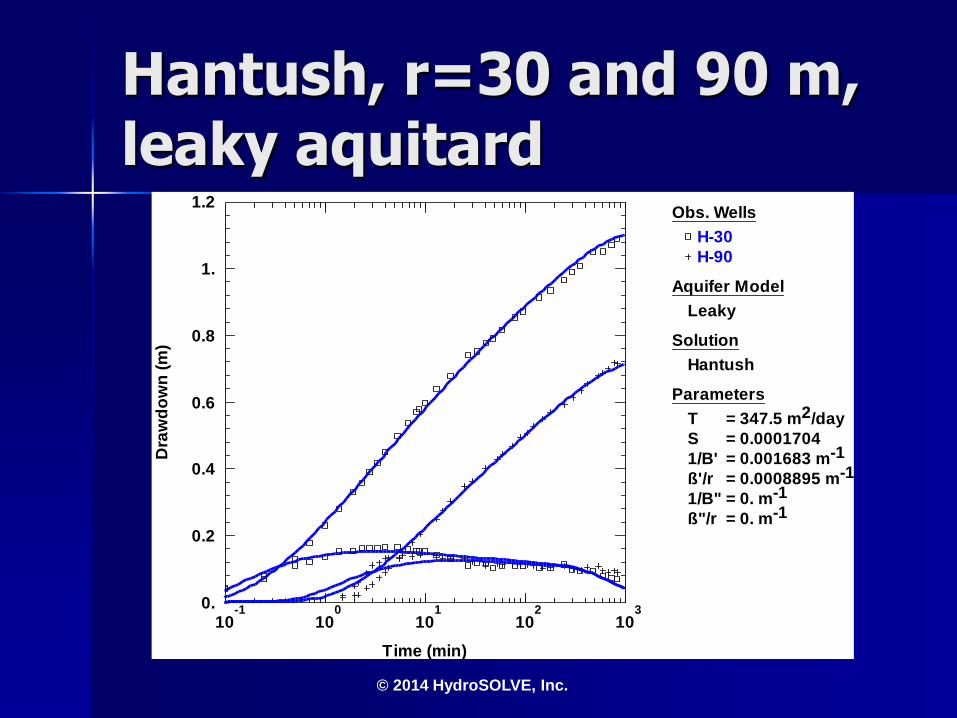
Hantush, r=30 and 90 m, leaky aquitard
10-1
100
101
102
1030.
0.2
0.4
0.6
0.8
1.
1.2
Time (min)
Dra
wd
ow
n (
m)
Obs. Wells
H-30
H-90
Aquifer Model
Leaky
Solution
Hantush
Parameters
T = 347.5 m2/day
S = 0.0001704
1/B' = 0.001683 m-1
ß'/r = 0.0008895 m-1
1/B" = 0. m-1
ß"/r = 0. m-1

© 2014 HydroSOLVE, Inc.
Hantush, r=30 and 90 m, leaky aquitard
10-1
100
101
102
10310
-2
10-1
100
101
Time (min)
Dra
wd
ow
n (
m)
Obs. Wells
H-30
H-90
Aquifer Model
Leaky
Solution
Hantush
Parameters
T = 347.5 m2/day
S = 0.0001704
1/B' = 0.001683 m-1
ß'/r = 0.0008895 m-1
1/B" = 0. m-1
ß"/r = 0. m-1

© 2014 HydroSOLVE, Inc.
Summary of Results
Estimates of T (leaky confined):
– 348 m2/day (compressible aquitard)
Estimates of T (nonleaky confined):
– 375 m2/day (Cooper-Jacob, early)
– 437 m2/day (Cooper-Jacob, composite)
– 600 m2/day (Cooper-Jacob, late)
© 2014 HydroSOLVE, Inc.
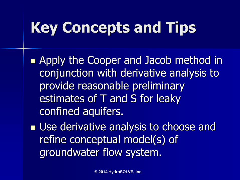
Key Concepts and Tips
Apply the Cooper and Jacob method in conjunction with derivative analysis to provide reasonable preliminary estimates of T and S for leaky confined aquifers.
Use derivative analysis to choose and refine conceptual model(s) of groundwater flow system.
© 2014 HydroSOLVE, Inc.
Case Study: Channel Aquifer Estevan, Saskatchewan
Walton (1970) presented data and results from an eight-day pumping test conducted in a buried sand-and-gravel channel aquifer near Estevan, Saskatchewan, Canada
– Q = 457 to 464 imperial gallons-per-minute
– b = 30 to 90 ft (typical)
– width of channel = 3,000 to 12,000 ft (typical)

© 2014 HydroSOLVE, Inc.
Well Locations
three observation wells
– r = 84 ft
– r = 250 ft
– r = 729 ft
from Walton (1970)
© 2014 HydroSOLVE, Inc.
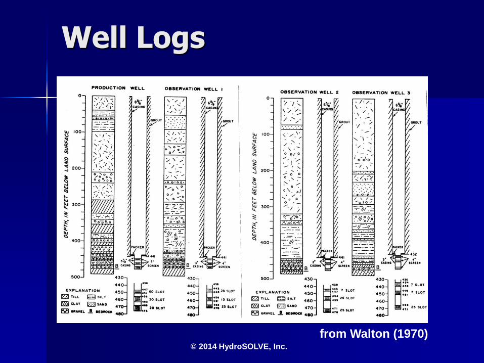
Well Logs
from Walton (1970)

© 2014 HydroSOLVE, Inc.
Walton’s Analysis
10-1
100
101
102
103
104
10510
-2
10-1
100
101
102
Time (min)
Dra
wd
ow
n (
ft)
Obs. Wells
PW
OW 1
OW 2
OW 3
Aquifer Model
Confined
Solution
Theis
Parameters
T = 3.02E+4 ft2/day
S = 0.00022
Kz/Kr = 1.
b = 50. ft
Walton only used a few
early-time observations
from OW3 in his
analysis…

© 2014 HydroSOLVE, Inc.
Composite Plot
10-7
10-5
10-3
10-1
101
103
1050.
4.
8.
12.
16.
20.
Time, t/r2 (min/ft2)
Dra
wd
ow
n (
ft)
all wells show same
slope at intermediate
time suggesting
infinite-acting aquifer
conditions
© 2014 HydroSOLVE, Inc.
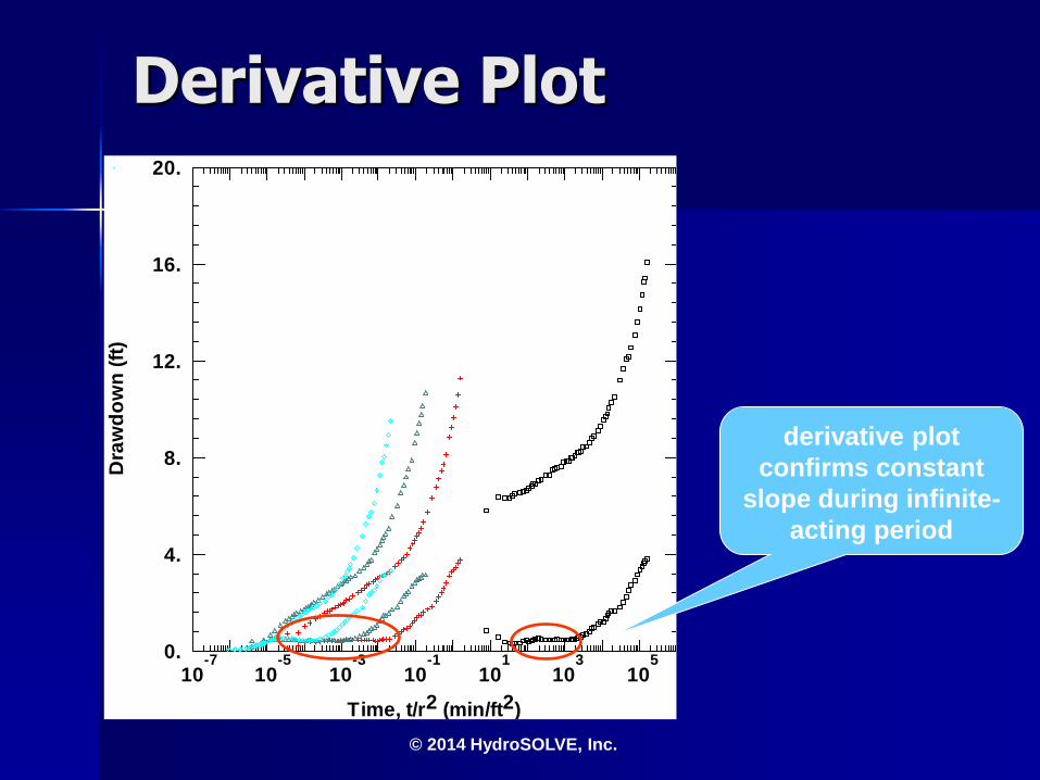
Derivative Plot
10-7
10-5
10-3
10-1
101
103
1050.
4.
8.
12.
16.
20.
Time, t/r2 (min/ft2)
Dra
wd
ow
n (
ft)
derivative plot
confirms constant
slope during infinite-
acting period

© 2014 HydroSOLVE, Inc.
Cooper and Jacob Match
10-7
10-5
10-3
10-1
101
103
1050.
4.
8.
12.
16.
20.
Time, t/r2 (min/ft2)
Dra
wd
ow
n (
ft)
Obs. Wells
PW
OW 1
OW 2
OW 3
Aquifer Model
Confined
Solution
Cooper-Jacob
Parameters
T = 1.983E+4 ft2/day
S = 0.0002836
aquifer properties
determined from
infinite-acting
period
© 2014 HydroSOLVE, Inc.
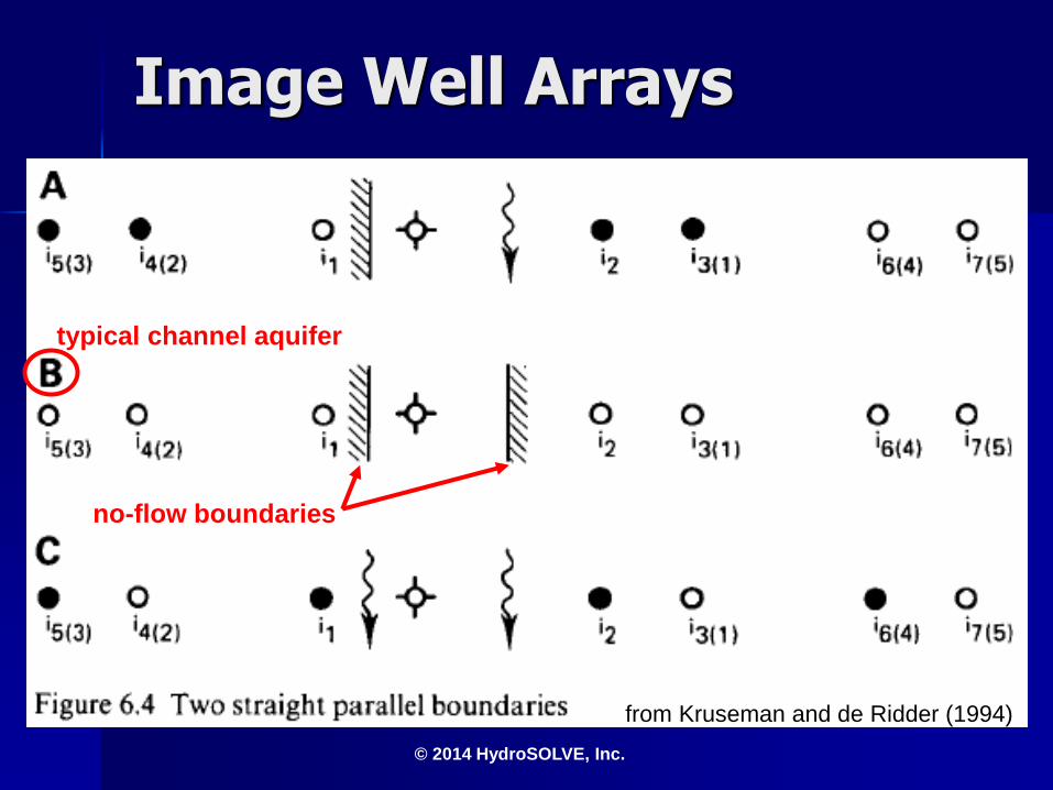
Image Well Arrays
from Kruseman and de Ridder (1994)
typical channel aquifer
no-flow boundaries

© 2014 HydroSOLVE, Inc.
Theis Analysis w/Channel
10-7
10-5
10-3
10-1
101
103
1050.
4.
8.
12.
16.
20.
Time, t/r2 (min/ft2)
Dra
wd
ow
n (
ft)
Obs. Wells
PW
OW 1
OW 2
OW 3
Aquifer Model
Confined
Solution
Theis
Parameters
T = 1.983E+4 ft2/day
S = 0.0002836
Kz/Kr = 1.
b = 50. ft
estimated channel
width = 8000 ft

© 2014 HydroSOLVE, Inc.
Key Concepts and Tips
Buried channel aquifer inferred from late-time derivative response
Aquifer properties (T and S) estimated efficiently from the infinite-acting period with composite plot and Cooper and Jacob solution
Channel width identified easily by trial-and-error using Theis solution and image wells
© 2014 HydroSOLVE, Inc.
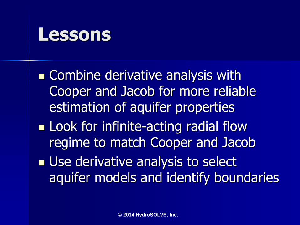
Lessons
Combine derivative analysis with Cooper and Jacob for more reliable estimation of aquifer properties
Look for infinite-acting radial flow regime to match Cooper and Jacob
Use derivative analysis to select aquifer models and identify boundaries

© 2014 HydroSOLVE, Inc.
Lessons
When applied carefully, Cooper and Jacob can provide reliable estimates of T and S in confined aquifers with or without leakage
Do not rely on Cooper and Jacob to determine S from single-well tests due to well loss