using decision rules to create retirement withdrawal...

You are here: FPA Net > FPA Journal > Past Issues & Articles > 2007 Issues > 2007 August Issue - Article 8

Return to normal view

Contribution Using Decision Rules to Create Retirement Withdrawal Profiles by William J. Klinger

Executive Summary

This paper describes an approach where retirees define their desired retirement withdrawal profiles and then establish rules for retirement asset withdrawals to maximize total purchasing power. This approach allows retirees to control their retirement; they are no longer subject to one-size-fits-all withdrawal strategies or rules of thumb. The implicit rules that financial planners use to guide portfolio withdrawals can be made explicit and tested for their effectiveness. The paper defines three primary retirement profiles. Under the uniform profile, withdrawals are steady throughout retirement; the progressive profile exhibits increased withdrawals in real dollars; and under the aggressive profile retirees make larger withdrawals early in retirement, followed by decreasing amounts. The paper illustrates all three profiles using a $1 million portfolio over a 40-year retirement period. After a retiree chooses the profile and the success rate that fits his or her retirement outlook, three decision rules can be applied to govern the amount withdrawn annually from investment assets and ideally boost the amounts safely withdrawn each year. The decision rules are drawn from the work of Jonathan Guyton and William Klinger: the Modified Withdrawal, Capital Preservation, and Prosperity rules. Using decision rules dramatically increases the present value of the total withdrawals over scenarios with no decision rules, while still achieving a 99 percent success rate. For example, a uniform withdrawal profile can be created using a safe initial withdrawal rate of 5.3 percent for a 40-year retirement period, versus 2.5 percent with no decision rules.

William J. Klinger teaches business and computer science at Raritan Valley Community College in North Branch, New Jersey. He can be reached at [email protected]. The majority of recent research on retirement spending attempts to answer the question, What is the maximum safe withdrawal rate for retired individuals? The answer has classically been to specify an initial withdrawal rate and assume that withdrawals in later years are adjusted for inflation (Bengen 1994, Bengen 1996, Bengen 1997). Recent research (Guyton 2004, Schlegel 2005, Guyton and Klinger 2006) has introduced the idea of using decision rules to adjust the withdrawal rate in a given year according to well-defined guidelines. A problem with the existing research is that from the viewpoint of retirees the process is backward. Withdrawal rates are defined and retirees are forced to fit their lifestyles to the resulting withdrawal stream. A more natural approach would be for retirees to specify their desired retirement withdrawal profile and have annual withdrawal rates defined to produce that profile. This paper defines three retirement withdrawal profiles and specifies decision rules that will produce each profile.

Past Research

A number of initialisms are defined and used in this paper. For quick reference, they are summarized in Table 1. Complete definitions follow in subsequent sections of this paper. Inputs to the model are shown in italics, outputs in normal font.

of 12FPA Journal - Using Decision Rules to Create Retirement Withdrawal Profiles

8/8/2007http://www.fpanet.org/journal/articles/2007_Issues/jfp0807-art8.cfm?renderforprint=1

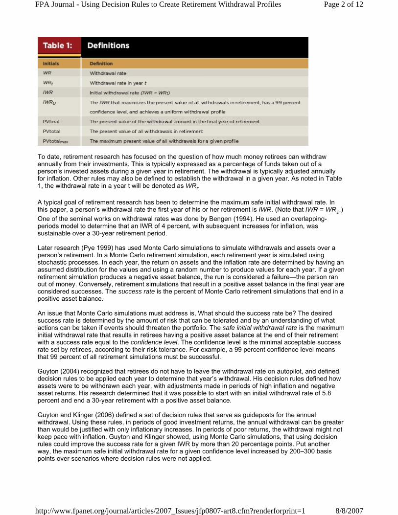
To date, retirement research has focused on the question of how much money retirees can withdraw annually from their investments. This is typically expressed as a percentage of funds taken out of a person’s invested assets during a given year in retirement. The withdrawal is typically adjusted annually for inflation. Other rules may also be defined to establish the withdrawal in a given year. As noted in Table 1, the withdrawal rate in a year t will be denoted as WRt. A typical goal of retirement research has been to determine the maximum safe initial withdrawal rate. In this paper, a person’s withdrawal rate the first year of his or her retirement is IWR. (Note that IWR = WR1.) One of the seminal works on withdrawal rates was done by Bengen (1994). He used an overlapping-periods model to determine that an IWR of 4 percent, with subsequent increases for inflation, was sustainable over a 30-year retirement period. Later research (Pye 1999) has used Monte Carlo simulations to simulate withdrawals and assets over a person’s retirement. In a Monte Carlo retirement simulation, each retirement year is simulated using stochastic processes. In each year, the return on assets and the inflation rate are determined by having an assumed distribution for the values and using a random number to produce values for each year. If a given retirement simulation produces a negative asset balance, the run is considered a failure—the person ran out of money. Conversely, retirement simulations that result in a positive asset balance in the final year are considered successes. The success rate is the percent of Monte Carlo retirement simulations that end in a positive asset balance. An issue that Monte Carlo simulations must address is, What should the success rate be? The desired success rate is determined by the amount of risk that can be tolerated and by an understanding of what actions can be taken if events should threaten the portfolio. The safe initial withdrawal rate is the maximum initial withdrawal rate that results in retirees having a positive asset balance at the end of their retirement with a success rate equal to the confidence level. The confidence level is the minimal acceptable success rate set by retirees, according to their risk tolerance. For example, a 99 percent confidence level means that 99 percent of all retirement simulations must be successful. Guyton (2004) recognized that retirees do not have to leave the withdrawal rate on autopilot, and defined decision rules to be applied each year to determine that year’s withdrawal. His decision rules defined how assets were to be withdrawn each year, with adjustments made in periods of high inflation and negative asset returns. His research determined that it was possible to start with an initial withdrawal rate of 5.8 percent and end a 30-year retirement with a positive asset balance. Guyton and Klinger (2006) defined a set of decision rules that serve as guideposts for the annual withdrawal. Using these rules, in periods of good investment returns, the annual withdrawal can be greater than would be justified with only inflationary increases. In periods of poor returns, the withdrawal might not keep pace with inflation. Guyton and Klinger showed, using Monte Carlo simulations, that using decision rules could improve the success rate for a given IWR by more than 20 percentage points. Put another way, the maximum safe initial withdrawal rate for a given confidence level increased by 200–300 basis points over scenarios where decision rules were not applied.



Present Research

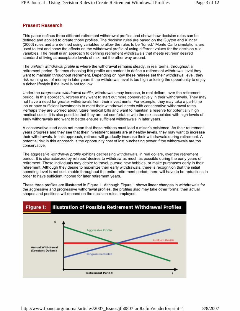
This paper defines three different retirement withdrawal profiles and shows how decision rules can be defined and applied to create those profiles. The decision rules are based on the Guyton and Klinger (2006) rules and are defined using variables to allow the rules to be “tuned.” Monte Carlo simulations are used to test and show the effects on the withdrawal profile of using different values for the decision rule variables. The result is an approach to defining retirement withdrawals that meets retirees’ desired standard of living at acceptable levels of risk, not the other way around. The uniform withdrawal profile is where the withdrawal remains steady, in real terms, throughout a retirement period. Retirees choosing this profile are content to define a retirement withdrawal level they want to maintain throughout retirement. Depending on how these retirees set their withdrawal level, they risk running out of money in later years if the withdrawal level is too high or losing the opportunity to enjoy a richer lifestyle if the level is set too low. Under the progressive withdrawal profile, withdrawals may increase, in real dollars, over the retirement period. In this approach, retirees may want to start out more conservatively in their withdrawals. They may not have a need for greater withdrawals from their investments. For example, they may take a part-time job or have sufficient investments to meet their withdrawal needs with conservative withdrawal rates. Perhaps they are worried about future medical bills and want to maintain a reserve for potentially high medical costs. It is also possible that they are not comfortable with the risk associated with high levels of early withdrawals and want to better ensure sufficient withdrawals in later years. A conservative start does not mean that these retirees must lead a miser’s existence. As their retirement years progress and they see that their investment assets are at healthy levels, they may want to increase their withdrawals. In this approach, retirees will gradually increase their withdrawals during retirement. A potential risk in this approach is the opportunity cost of lost purchasing power if the withdrawals are too conservative. The aggressive withdrawal profile exhibits decreasing withdrawals, in real dollars, over the retirement period. It is characterized by retirees’ desires to withdraw as much as possible during the early years of retirement. These individuals may desire to travel, pursue new hobbies, or make purchases early in their retirement. Although they desire to maximize their early withdrawals, there is recognition that the initial spending level is not sustainable throughout the entire retirement period; there will have to be reductions in order to have sufficient income for later retirement years. These three profiles are illustrated in Figure 1. Although Figure 1 shows linear changes in withdrawals for the aggressive and progressive withdrawal profiles, the profiles also may take other forms; their actual shapes and positions will depend on the decision rules employed.



Decision Rules

Guyton and Klinger (2006) showed that using decision rules to modify withdrawals can result in significantly higher total withdrawals than one could achieve with only increases for inflation, with the same success rate. Two of their decision rules are designed to protect retirees’ investment assets from running out. Obviously, poor investment returns alone will reduce investments. Investments also could be depleted during periods of high inflation relative to investment returns. To protect against running out of money, the following decision rules were defined: Modified Withdrawal Rule. Withdrawals increase from year to year with the inflation rate, except there is no increase following a year where the retirement portfolio’s total return is negative and when that year’s withdrawal rate would be greater than the initial withdrawal rate. There is no make-up for a missed increase. Capital Preservation Rule. If the withdrawal rate in any year t would exceed the initial withdrawal rate, IWR, by a percentage greater than Exceeds, the withdrawal rate for that year is cut by a percentage Cut. That is,

if (WRt / IWR – 1) > Exceeds, then set WRt to (1 – Cut) × WRt.

Exceeds and Cut are variables set by the retiree or planner. Possible values for these variables are discussed later in this paper. This rule is not applied during the final 15 years of the anticipated retirement period. Guyton and Klinger (2006) found that this restriction increased the total amount of withdrawals during the retirement period without a significant decrease in the success rate. As an example, assume that a person retires with $1 million in investments and chooses an initial withdrawal of $50,000. That person’s initial withdrawal rate is 5 percent. In a future year, if inflation and investment returns result in that person’s investments equaling $1,250,000 and their nominal withdrawal is $75,625, then their withdrawal rate in that year, WRt, is 75,625 / 1,250,000 = .0605 or 6.05 percent. This exceeds the initial withdrawal rate by 21 percent ((.0605 / .05) – 1 = .21). If the Capital Preservation Rule is defined with Exceeds = 20% and Cut = 10%, then the Capital Preservation Rule would be applied because .21 > .20. The withdrawal in that year would be cut to (1 – Cut) × Withdrawal = (1 – .10) × $75,625 = $68,062. If Exceeds and Cut are appropriately defined, withdrawals can be adjusted moderatelyto protect future portfolio value. The Modified Withdrawal Rule and Capital Preservation Rule help retirees avoid running out of money. The converse situation could occur when retirees’ investment returns are very good compared with inflation. In this case, retirees might want to, in effect, give themselves a raise. To guide this decision, the following rule was defined: Prosperity Rule. If the withdrawal rate in any year should fall below the initial withdrawal rate by more than a percentage Fall, the withdrawal is increased by a percentage Raise. That is, if (1 – WRt / IWR) > Fall, then set WRt to (1 + Raise) × WRt .

Fall and Raise are variables, which will be set by the retiree or planner. Possible values for them are discussed later. Again starting with an initial $1 million in investments and an initial withdrawal rate of 5 percent, assume a person will use the Prosperity Rule defined with Fall = 20% and Raise = 10%. If a series of bull markets and low inflation results in investments totaling $2 million and a current withdrawal amount of $79,000, the withdrawal rate in that year is only $79,000 / $2,000,000 = 3.95%, which is (1 – .0395 / .05) = .21, or 21 percent below the initial withdrawal rate of 5 percent. The Prosperity Rule is applied because the 21 percent drop is greater than our Fall = 20% and the withdrawal for that year is adjusted upward to (1 + Raise) × WithdrawalAmount = (1 + .10) × $79,000 = $86,900. The effect is a raise in real withdrawals. If Fall and Raise are reasonably defined, the withdrawal will not become dangerously high.



The remainder of this paper discusses the determination of the appropriate values for IWR and the variables (Exceeds, Cut, Fall, and Raise) in the decision rules to achieve the desired retirement withdrawalprofile.

Approach and Simulator

The approach taken in this research applies Monte Carlo techniques to simulate retirees’ portfolios during their retirement. A Monte Carlo simulator written in C++ was used to simulate retirement portfolios. The base assumptions of the simulator are the length of the retirement period, the amount of initial retirement assets, the asset allocation, the asset return distributions, and the inflation rate distribution. A conservative 40-year retirement period was chosen to simulate retirements because many people are retiring earlier and living longer. There is nothing magical about 40 years; results are also shown for a 30-year retirement period. This research assumes a retirement portfolio of $1 million with an asset allocation of 60 percent equities, 30 percent bonds, and 10 percent cash. Each year’s entire withdrawal is made from the portfolio’s assets on the first day of the simulated year. Withdrawals rise annually by the prior year’s inflation rate, modified by any decision rules in effect using the formulas presented earlier, and are deducted from the retirement assets. At that time, the asset classes are rebalanced to the target asset allocation. (Earlier work by Guyton and Klinger (2006) used the Portfolio Management Decision Rule and did not rebalance assets each year. That rule does not materiallyaffect the shape of a retirement profile and simple rebalancing was used for this research.) Asset returns are calculated at the end of each simulated year. Asset return relatives (defined to be 1 + r, where r is the simple rate of return) are assumed to be lognormally distributed (Ibbotson & Associates 2005). Asset returns are based upon historical performance over the period of 1926 to 2004 (AXA). To use this approach, the natural logarithm of the return relative for each year in the period is calculated. The mean and standard deviation are then calculated from those values over the period sample. Stocks are represented by the total returns of the S&P 500, with a lognormal return relative mean of 9.62 percent and a standard deviation of 19.5 percent. For bonds, total returns of long-term Treasuries are used and the values are 4.99 percent and 6.96 percent. Three-month T-bills are the basis for cash returns and the values are 3.74 percent and 2.98 percent. Inflation is modeled in the same manner using the Consumer Price Index over the period of 1926 to 2004 (FRED®), with a mean of 3.13 percent and a standard deviation of 4.16 percent. For each year, the simulated return is obtained by generating a random number from the lognormal distribution with the appropriate mean and standard deviation and raising the mathematical constant e to that power to get the return relative. Retirees’ portfolios are simulated by performing the above calculations for each retirement year, such as 40 times for an assumed retirement of 40 years. If the sum of all assets becomes negative during a simulated lifetime, the simulation is considered a failure. A retirement scenario is defined by a given set of initial values (IWR, Exceeds, Cut, Fall, and Raise) and base assumptions. Each scenario is run 1,000 times and the success rate of a scenario is the percent of successful simulations. The simulator is robust and allows decision rules to be turned on or off and base assumptions to be changed for each scenario. An important consideration in trying to establish a retirement withdrawal profile is what level of risk is the retiree comfortable with. Confidence levels for withdrawal scenarios not using decision rules might use a 90 percent success rate or even an 85 percent success rate. This is due in part to the unstated assumption that if a portfolio gets into trouble, actions will be taken to rescue the portfolio. When the withdrawals become high relative to the retirement assets and threaten the sustainability of the portfolio, retirees may be forced to decrease their withdrawals, take a part-time job, or reduce their expenses. The analysis in this paper does not take into account actions such as taking a job, but does make explicit cuts in withdrawals using the Capital Preservation Rule and freezes using the Modified Withdrawal Rule. These cuts and freezes are no longer fallback options; therefore, the analysis here raises the confidence level to a 99 percent success rate. The simulator outputs of interest are



1. PVfinal: The present value of the withdrawal amount in the final year of retirement. The discount rate used in the PVfinal calculations is the inflation rate observed in each year of retirement.

2. PVtotal: The present value of the sum of all the withdrawals made during the retirement period. PVtotal is the total purchasing power, in constant dollars, over a retirement period. This number allows for comparisons between different scenarios and it is assumed that retirees prefer to maximize their withdrawals during retirement. The discount rate used in the PVtotal calculations is, again, the inflation rate observed in each year.

3. The success rate: In any profile, this number must not fall below the desired confidence level.

In 1,000 scenario simulations there will be 1,000 PVtotal and PVfinal values. To avoid having a few high values distort the results, the median values are used in the analysis. Median values are calculated for only successful simulations, and since a 99 percent confidence level is used, this will, for all practical purposes, be the median for all simulations. The simulator is used to test different scenarios. It is first used to establish the relationship between each of the five decision rule variables (IWR, Exceeds, Cut, Fall, and Raise) and the simulator outputs (PVtotal, PVfinal, and the success rate). This is done by running the simulator several times holding all but one of the decision rule variables constant and seeing the effect on the outputs. This gives a directional relationship between the input variables and outputs. Once the directional relationship between the decision rule variables and the simulator outputs is established, it is used to modify the profile of retirementwithdrawals. Note that although the success rate is an output, retirees define up front their minimum acceptable success rate, their confidence level; therefore, only scenarios that meet the confidence level are considered. Although this research uses Monte Carlo techniques, there is no inherent reason that an overlapping-periods model cannot be used. Likewise, Monte Carlo simulations using different asset allocations and more than three asset classes also can be used. Although the specific success rates will change, the fundamental direction and control of the decision rules will not change.

Results

The first step is to determine the impact of the defined initial values on the present values and the success rate. Starting with $1 million in investment assets, if no decision rules are applied, a 99 percent success rate is achieved with an initial withdrawal rate of 2.5 percent, which is a withdrawal of $25,000. Continuing to withdraw $25,000 in real dollars over 40 years results in a PVtotal of $1 million. When the IWR is increased and all other variables are held constant, more will be withdrawn over the retirement period and both present values will rise. In this case, raising the IWR to 3.05 percent raises the PVfinal to $30,500 and PVtotal to $1,220,000; however, the success rate decreases to 95 percent. When the Modified Withdrawal Rule is applied to the above case with an initial withdrawal rate of 5 percent, the success rate improves to 100 percent. This is expected because the Modified Withdrawal Rule does not increase the withdrawal in periods of negative market returns. Applying the Modified Withdrawal Rule also will lower the present values. In this example, the PVfinal decreases to $24,817 and the PVtotal falls to $998,000. Applying only the Capital Preservation Rule with Exceeds = 20% and Cut = 10% achieves a 99 percent success rate at an initial withdrawal rate of 5.25 percent, yielding a PVfinal of $42,444 and a PVtotal of $1,772,000. Raising the rule threshold Exceeds to 40 percent, the success rate drops to 95 percent, while the PVfinal rises to $47,160 and the PVtotal rises to $1,921,000. Increasing the amount of a Cut to 20 percent has the opposite effect. In this case, the success rate rises to 100 percent, while the PVfinal decreases to $41,920 and the PVtotal falls to $1,708,000. Applying only the Prosperity Rule with Fall = 20% and Raise = 10% has a 99 percent success rate with an initial withdrawal rate of 2.5 percent. It gives a PVfinal of $70,757 and a PVtotal of $1,665,000. Raising the threshold to Fall = 40% means that retirees will have fewer raise opportunities. In this scenario, the PVfinal drops to $53,161 and the PVtotal falls to $1,381,000; the success rate does not change. The success rate did not change for IWR = 2.5% because the success rate was already 99 percent and the scenario failureswere not due to raises. But increasing Fall does increase the success rates for higher initial withdrawal rates, and the safe IWR in this case increases to 2.6 percent. The effect of setting Raise at 20 percent



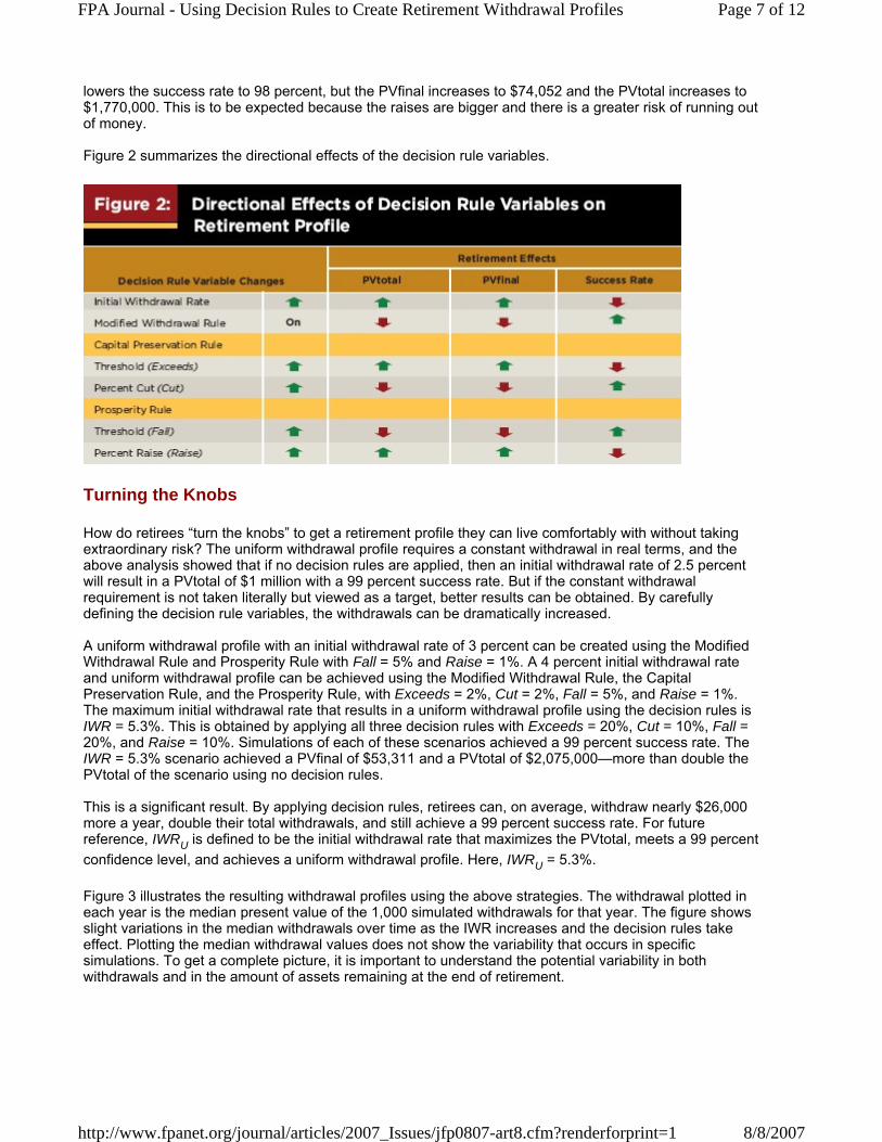
lowers the success rate to 98 percent, but the PVfinal increases to $74,052 and the PVtotal increases to $1,770,000. This is to be expected because the raises are bigger and there is a greater risk of running out of money. Figure 2 summarizes the directional effects of the decision rule variables.

Turning the Knobs

How do retirees “turn the knobs” to get a retirement profile they can live comfortably with without taking extraordinary risk? The uniform withdrawal profile requires a constant withdrawal in real terms, and the above analysis showed that if no decision rules are applied, then an initial withdrawal rate of 2.5 percent will result in a PVtotal of $1 million with a 99 percent success rate. But if the constant withdrawal requirement is not taken literally but viewed as a target, better results can be obtained. By carefully defining the decision rule variables, the withdrawals can be dramatically increased. A uniform withdrawal profile with an initial withdrawal rate of 3 percent can be created using the Modified Withdrawal Rule and Prosperity Rule with Fall = 5% and Raise = 1%. A 4 percent initial withdrawal rate and uniform withdrawal profile can be achieved using the Modified Withdrawal Rule, the Capital Preservation Rule, and the Prosperity Rule, with Exceeds = 2%, Cut = 2%, Fall = 5%, and Raise = 1%. The maximum initial withdrawal rate that results in a uniform withdrawal profile using the decision rules is IWR = 5.3%. This is obtained by applying all three decision rules with Exceeds = 20%, Cut = 10%, Fall = 20%, and Raise = 10%. Simulations of each of these scenarios achieved a 99 percent success rate. The IWR = 5.3% scenario achieved a PVfinal of $53,311 and a PVtotal of $2,075,000—more than double the PVtotal of the scenario using no decision rules. This is a significant result. By applying decision rules, retirees can, on average, withdraw nearly $26,000 more a year, double their total withdrawals, and still achieve a 99 percent success rate. For future reference, IWRU is defined to be the initial withdrawal rate that maximizes the PVtotal, meets a 99 percent confidence level, and achieves a uniform withdrawal profile. Here, IWRU = 5.3%. Figure 3 illustrates the resulting withdrawal profiles using the above strategies. The withdrawal plotted in each year is the median present value of the 1,000 simulated withdrawals for that year. The figure shows slight variations in the median withdrawals over time as the IWR increases and the decision rules take effect. Plotting the median withdrawal values does not show the variability that occurs in specific simulations. To get a complete picture, it is important to understand the potential variability in both withdrawals and in the amount of assets remaining at the end of retirement.



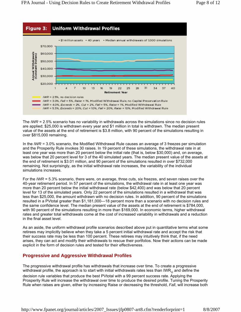
The IWR = 2.5% scenario has no variability in withdrawals across the simulations since no decision rules are applied; $25,000 is withdrawn every year and $1 million in total is withdrawn. The median present value of the assets at the end of retirement is $3.8 million, with 90 percent of the simulations resulting in over $815,000 remaining. In the IWR = 3.0% scenario, the Modified Withdrawal Rule causes an average of 3 freezes per simulation and the Prosperity Rule invokes 30 raises. In 19 percent of these simulations, the withdrawal rate in at least one year was more than 20 percent below the initial rate (that is, below $30,000) and, on average, was below that 20 percent level for 3 of the 40 simulated years. The median present value of the assets at the end of retirement is $3.01 million, and 90 percent of the simulations resulted in over $732,000 remaining. Not surprisingly, as the initial withdrawal rate increases, the variability of the individual simulations increases. For the IWR = 5.3% scenario, there were, on average, three cuts, six freezes, and seven raises over the 40-year retirement period. In 57 percent of the simulations, the withdrawal rate in at least one year was more than 20 percent below the initial withdrawal rate (below $42,400) and was below that 20 percent level for 13 of the simulated years. Only 22 percent of the simulations resulted in a withdrawal that was less than $25,000, the amount withdrawn with no decision rules. In addition, 90 percent of the simulations resulted in a PVtotal greater than $1,181,000—18 percent more than a scenario with no decision rules and the same confidence level. The median present value of the assets at the end of retirement is $784,000, with 90 percent of the simulations resulting in more than $169,000. In economic terms, higher withdrawal rates and greater total withdrawals come at the cost of increased variability in withdrawals and a reduction in the final asset level. As an aside, the uniform withdrawal profile scenarios described above put in quantitative terms what some retirees may implicitly believe when they take a 5 percent initial withdrawal rate and accept the risk that their success rate may be less than 100 percent. These retirees may intuitively think that, if the need arises, they can act and modify their withdrawals to rescue their portfolios. Now their actions can be made explicit in the form of decision rules and tested for their effectiveness.

Progressive and Aggressive Withdrawal Profiles

The progressive withdrawal profile has withdrawals that increase over time. To create a progressive withdrawal profile, the approach is to start with initial withdrawals rates less than IWRU and define the decision rule variables that produce the best PVtotal with a 99 percent success rate. Applying the Prosperity Rule will increase the withdrawal over time to produce the desired profile. Tuning the Prosperity Rule when raises are given, either by increasing Raise or decreasing the threshold, Fall, will increase both



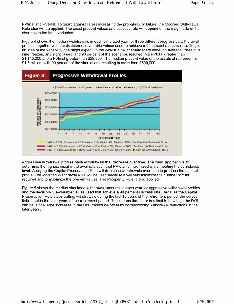
PVfinal and PVtotal. To guard against raises increasing the probability of failure, the Modified Withdrawal Rule also will be applied. The exact present values and success rate will depend on the magnitude of the changes to the input variables. Figure 4 shows the median withdrawals in each simulated year for three different progressive withdrawal profiles, together with the decision rule variable values used to achieve a 99 percent success rate. To get an idea of the variability one might expect, in the IWR = 3.2% scenario there were, on average, three cuts, nine freezes, and eight raises, and 90 percent of the scenarios resulted in a PVtotal greater than $1,110,000 and a PVfinal greater than $28,500. The median present value of the assets at retirement is $1.7 million, with 90 percent of the simulations resulting in more than $590,000.

Aggressive withdrawal profiles have withdrawals that decrease over time. The basic approach is to determine the highest initial withdrawal rate such that PVtotal is maximized while meeting the confidence level. Applying the Capital Preservation Rule will decrease withdrawals over time to produce the desired profile. The Modified Withdrawal Rule will be used because it will help minimize the number of cuts required and to maximize the present values. The Prosperity Rule is also applied. Figure 5 shows the median simulated withdrawal amounts in each year for aggressive withdrawal profiles and the decision-rule-variable values used that achieve a 99 percent success rate. Because the Capital Preservation Rule stops cutting withdrawals during the last 15 years of the retirement period, the curves flatten out in the later years of the retirement period. This means that there is a limit to how high the IWR can be, since large increases in the IWR cannot be offset by corresponding withdrawal reductions in the later years.



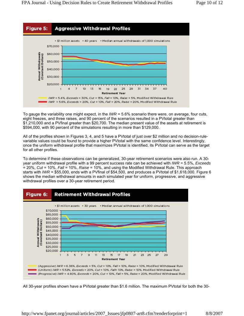
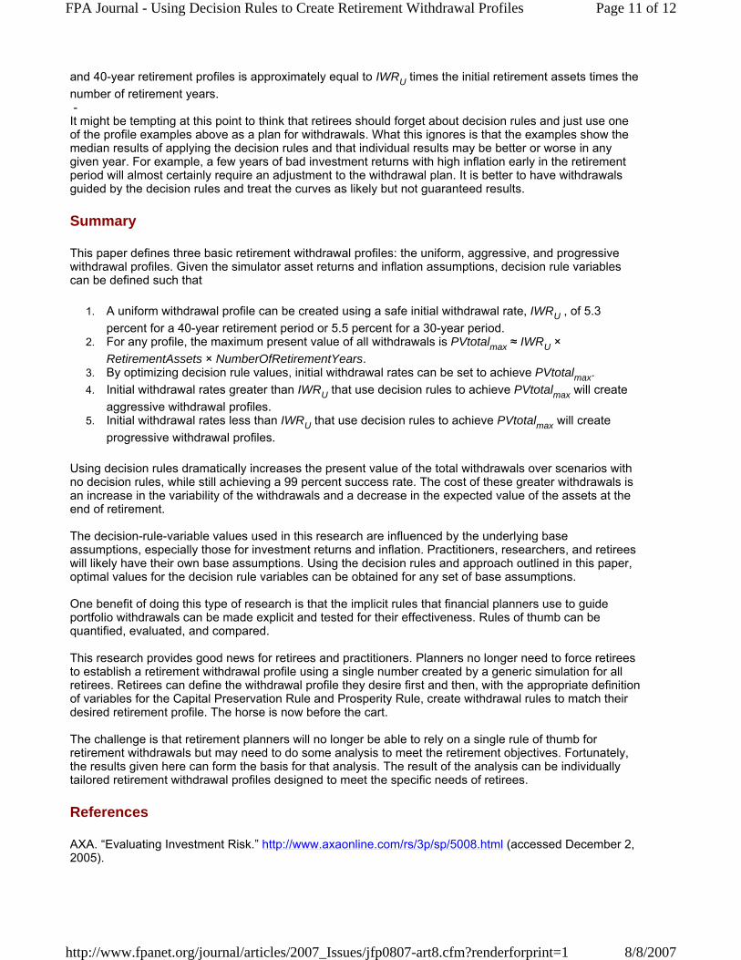
To gauge the variability one might expect, in the IWR = 5.6% scenario there were, on average, four cuts, eight freezes, and three raises, and 90 percent of the scenarios resulted in a PVtotal greater than $1,210,000 and a PVfinal greater than $20,700. The median present value of the assets at retirement is $594,000, with 90 percent of the simulations resulting in more than $129,000. All of the profiles shown in Figures 3, 4, and 5 have a PVtotal of just over $2 million and no decision-rule-variable values could be found to provide a higher PVtotal with the same confidence level. Interestingly, once the uniform withdrawal profile that maximizes PVtotal is identified, its PVtotal can serve as the target for all other profiles. To determine if these observations can be generalized, 30-year retirement scenarios were also run. A 30-year uniform withdrawal profile with a 99 percent success rate can be achieved with IWR = 5.5%, Exceeds= 20%, Cut = 10%, Fall = 10%, Raise = 10%, and using the Modified Withdrawal Rule. This approach starts with IWR = $55,000, ends with a PVfinal of $54,500, and produces a PVtotal of $1,618,000. Figure 6 shows the median withdrawal amounts in each simulated year for uniform, progressive, and aggressive withdrawal profiles over a 30-year retirement period.

All 30-year profiles shown have a PVtotal greater than $1.6 million. The maximum PVtotal for both the 30-



and 40-year retirement profiles is approximately equal to IWRU times the initial retirement assets times the number of retirement years. - It might be tempting at this point to think that retirees should forget about decision rules and just use one of the profile examples above as a plan for withdrawals. What this ignores is that the examples show the median results of applying the decision rules and that individual results may be better or worse in any given year. For example, a few years of bad investment returns with high inflation early in the retirement period will almost certainly require an adjustment to the withdrawal plan. It is better to have withdrawals guided by the decision rules and treat the curves as likely but not guaranteed results.

Summary

This paper defines three basic retirement withdrawal profiles: the uniform, aggressive, and progressive withdrawal profiles. Given the simulator asset returns and inflation assumptions, decision rule variables can be defined such that

1. A uniform withdrawal profile can be created using a safe initial withdrawal rate, IWRU , of 5.3 percent for a 40-year retirement period or 5.5 percent for a 30-year period.

2. For any profile, the maximum present value of all withdrawals is PVtotalmax ≈ IWRU × RetirementAssets × NumberOfRetirementYears.

3. By optimizing decision rule values, initial withdrawal rates can be set to achieve PVtotalmax. 4. Initial withdrawal rates greater than IWRU that use decision rules to achieve PVtotalmax will create

aggressive withdrawal profiles. 5. Initial withdrawal rates less than IWRU that use decision rules to achieve PVtotalmax will create

progressive withdrawal profiles.

Using decision rules dramatically increases the present value of the total withdrawals over scenarios with no decision rules, while still achieving a 99 percent success rate. The cost of these greater withdrawals is an increase in the variability of the withdrawals and a decrease in the expected value of the assets at the end of retirement. The decision-rule-variable values used in this research are influenced by the underlying base assumptions, especially those for investment returns and inflation. Practitioners, researchers, and retirees will likely have their own base assumptions. Using the decision rules and approach outlined in this paper, optimal values for the decision rule variables can be obtained for any set of base assumptions. One benefit of doing this type of research is that the implicit rules that financial planners use to guide portfolio withdrawals can be made explicit and tested for their effectiveness. Rules of thumb can be quantified, evaluated, and compared. This research provides good news for retirees and practitioners. Planners no longer need to force retirees to establish a retirement withdrawal profile using a single number created by a generic simulation for all retirees. Retirees can define the withdrawal profile they desire first and then, with the appropriate definition of variables for the Capital Preservation Rule and Prosperity Rule, create withdrawal rules to match their desired retirement profile. The horse is now before the cart. The challenge is that retirement planners will no longer be able to rely on a single rule of thumb for retirement withdrawals but may need to do some analysis to meet the retirement objectives. Fortunately, the results given here can form the basis for that analysis. The result of the analysis can be individually tailored retirement withdrawal profiles designed to meet the specific needs of retirees.

References

AXA. “Evaluating Investment Risk.” http://www.axaonline.com/rs/3p/sp/5008.html (accessed December 2, 2005).



Bengen, William P. 1994. “Determining Withdrawal Rates Using Historical Data.” Journal of Financial Planning January: 14–24. Bengen, William P. 1996. “Asset Allocation for a Lifetime.” Journal of Financial Planning August: 58–67. Bengen, William P. 1997. “Conserving Client Portfolios During Retirement, Part III.” Journal of Financial Planning December: 84–97. Federal Reserve Bank of St. Louis Economic Data (FRED®). http://research.stlouisfed.org/fred2 (accessed December 2, 2005). Guyton, Jonathan T. 2004. “Decision Rules and Portfolio Management for Retirees: Is the ‘Safe’ Initial Withdrawal Rate Too Safe?” Journal of Financial Planning October: 54–62. Guyton, Jonathan T. and William J. Klinger. 2006. “Decision Rules and Maximum Initial Withdrawal Rates.” Journal of Financial Planning 19, 3 (March): 48–58. Ibbotson & Associates. 2005. Stocks, Bonds, Bills, and Inflation 2005 Yearbook. Chicago: Ibbotson & Associates, 164–165. Pye, Gordon B. 1999. “Sustainable Real Spending from Pensions and Investments.” Journal of Financial Planning June: 80–91. Schlegel, Jeff. 2005. “Time and Money.” Financial Advisor March: 57–60.



using decision rules to create retirement withdrawal...

Documents