using data mining to dynamically build up just in time
TRANSCRIPT

Using Data Mining To Dynamically
Build Up Just In Time Learner Models
A Thesis Submitted to the
College of Graduate Studies and Research
in Partial Fulfillment of the Requirements
for the Degree of Master of Science
in the Department of Computer Science
University of Saskatchewan
Saskatoon
By
Wengang Liu
c©Wengang Liu, December 2009. All rights reserved.

Permission to Use
In presenting this thesis in partial fulfilment of the requirements for a Postgrad-
uate degree from the University of Saskatchewan, I agree that the Libraries of this
University may make it freely available for inspection. I further agree that permission
for copying of this thesis in any manner, in whole or in part, for scholarly purposes
may be granted by the professor or professors who supervised my thesis work or, in
their absence, by the Head of the Department or the Dean of the College in which
my thesis work was done. It is understood that any copying or publication or use of
this thesis or parts thereof for financial gain shall not be allowed without my written
permission. It is also understood that due recognition shall be given to me and to the
University of Saskatchewan in any scholarly use which may be made of any material
in my thesis.
Requests for permission to copy or to make other use of material in this thesis in
whole or part should be addressed to:
Head of the Department of Computer Science
176 Thorvaldson Building
110 Science Place
University of Saskatchewan
Saskatoon, Saskatchewan
Canada
S7N 5C9
i

Abstract
Using rich data collected from e-learning systems, it may be possible to build up
just in time dynamic learner models to analyze learners’ behaviours and to evaluate
learners’ performance in online education systems. The goal is to create metrics
to measure learners’ characteristics from usage data. To achieve this goal we need
to use data mining methods, especially clustering algorithms, to find patterns from
which metrics can be derived from usage data. In this thesis, we propose a six layer
model (raw data layer, fact data layer, data mining layer, measurement layer, metric
layer and pedagogical application layer) to create a just in time learner model which
draws inferences from usage data. In this approach, we collect raw data from online
systems, filter fact data from raw data, and then use clustering mining methods to
create measurements and metrics.
In a pilot study, we used usage data collected from the iHelp system to create
measurements and metrics to observe learners’ behaviours in a real online system.
The measurements and metrics relate to a learner’s sociability, activity levels, learn-
ing styles, and knowledge levels. To validate the approach we designed two experi-
ments to compare the metrics and measurements extracted from the iHelp system:
expert evaluations and learner self evaluations. Even though the experiments did
not produce statistically significant results, this approach shows promise to describe
learners’ behaviours through dynamically generated measurements and metric. Con-
tinued research on these kinds of methodologies is promising.
ii

Acknowledgements
I am deeply grateful to my supervisor, Dr. Gord McCalla. Without his guidance,
understanding and patience, I would never complete writing this thesis.
Special thanks goes to many graduate students in ARIES lab, Scott, Zinan, Chris,
and Collene, who helped me get through the graduate study.
I would also like to thank my family, my wife Lirong and daughter Siqi, for their
encouragement and support.
iii

Contents
Permission to Use i
Abstract ii
Acknowledgements iii
Contents iv
List of Tables vii
List of Figures viii
List of Abbreviations xi
1 Introduction 1
1.1 Make Sense of Usage Data . . . . . . . . . . . . . . . . . . . . . . . . 1
1.2 Issues of Using Usage Data . . . . . . . . . . . . . . . . . . . . . . . . 2
1.3 Thesis Objectives . . . . . . . . . . . . . . . . . . . . . . . . . . . . . 3
1.4 Thesis Contributions . . . . . . . . . . . . . . . . . . . . . . . . . . . 3
1.5 Organization of Thesis . . . . . . . . . . . . . . . . . . . . . . . . . . 4
2 Literature Review 5
2.1 Learner Modelling for E-learning Systems . . . . . . . . . . . . . . . . 5
2.1.1 E-Learning . . . . . . . . . . . . . . . . . . . . . . . . . . . . 5
2.1.2 Learning Content Management Systems . . . . . . . . . . . . 6
2.1.3 Adaptive and Intelligent Web-based Educational Systems . . . 8
2.1.4 Learner Model . . . . . . . . . . . . . . . . . . . . . . . . . . . 10
2.2 Data Mining Algorithms . . . . . . . . . . . . . . . . . . . . . . . . . 11
2.2.1 The Definition of Data Mining . . . . . . . . . . . . . . . . . . 11
2.2.2 Data Mining Tasks . . . . . . . . . . . . . . . . . . . . . . . . 12
2.2.3 Categories of Data Mining Algorithms . . . . . . . . . . . . . 13
2.3 Educational Data Mining . . . . . . . . . . . . . . . . . . . . . . . . . 14
2.3.1 Data Mining Techniques in Educational Systems . . . . . . . . 15
2.3.2 Classification . . . . . . . . . . . . . . . . . . . . . . . . . . . 16
2.3.3 Association Rules . . . . . . . . . . . . . . . . . . . . . . . . . 17
2.3.4 Bayesian Network . . . . . . . . . . . . . . . . . . . . . . . . . 19
2.3.5 Clustering . . . . . . . . . . . . . . . . . . . . . . . . . . . . . 22
2.3.6 Regression . . . . . . . . . . . . . . . . . . . . . . . . . . . . . 29
2.3.7 Support Vector Machines . . . . . . . . . . . . . . . . . . . . . 30
iv

3 Dynamically Mining Learners’Characteristics 333.1 Motivation . . . . . . . . . . . . . . . . . . . . . . . . . . . . . . . . . 333.2 Data Collection . . . . . . . . . . . . . . . . . . . . . . . . . . . . . . 34
3.2.1 Raw Data . . . . . . . . . . . . . . . . . . . . . . . . . . . . . 353.2.2 Fact Data . . . . . . . . . . . . . . . . . . . . . . . . . . . . . 36
3.3 Purpose-Based Methods . . . . . . . . . . . . . . . . . . . . . . . . . 383.3.1 Pedagogical Purposes . . . . . . . . . . . . . . . . . . . . . . . 383.3.2 Methods Based on Purposes . . . . . . . . . . . . . . . . . . . 39
3.4 Dynamic Learner Model . . . . . . . . . . . . . . . . . . . . . . . . . 403.4.1 Model . . . . . . . . . . . . . . . . . . . . . . . . . . . . . . . 423.4.2 Layers . . . . . . . . . . . . . . . . . . . . . . . . . . . . . . . 433.4.3 Dynamic Procedure . . . . . . . . . . . . . . . . . . . . . . . . 46
3.5 Implementation of Dynamic Learner Modelling . . . . . . . . . . . . . 483.5.1 Selection of Raw Data and Fact Data . . . . . . . . . . . . . . 483.5.2 Selection of Data Mining Algorithms . . . . . . . . . . . . . . 503.5.3 Selection of Metrics and Measurements . . . . . . . . . . . . . 52
4 Analyzing the Metrics and Measurements 614.1 Introduction . . . . . . . . . . . . . . . . . . . . . . . . . . . . . . . . 614.2 Methods of Analysis . . . . . . . . . . . . . . . . . . . . . . . . . . . 62
4.2.1 Confusion Matrix . . . . . . . . . . . . . . . . . . . . . . . . . 624.2.2 Inter-rater reliability . . . . . . . . . . . . . . . . . . . . . . . 63
4.3 Experment I – Expert Evaluation . . . . . . . . . . . . . . . . . . . . 644.3.1 Experiment Information . . . . . . . . . . . . . . . . . . . . . 644.3.2 Expert Evaluation . . . . . . . . . . . . . . . . . . . . . . . . 684.3.3 Results Analysis . . . . . . . . . . . . . . . . . . . . . . . . . 704.3.4 Conclusion of Expert Evaluation . . . . . . . . . . . . . . . . 81
4.4 Experiment II – Learner Self Evaluation . . . . . . . . . . . . . . . . 824.4.1 Experiment Information . . . . . . . . . . . . . . . . . . . . . 824.4.2 Learner Self Evaluation . . . . . . . . . . . . . . . . . . . . . 824.4.3 Analysis of Results . . . . . . . . . . . . . . . . . . . . . . . . 84
4.5 Conclusions of Learner Self EvaluationExperiment . . . . . . . . . . . . . . . . . . . . . . . . . . . . . . . . 86
5 Research Contributionsand Future Directions 885.1 General Comments on the Two Experiments . . . . . . . . . . . . . . 88
5.1.1 Expert Experiment . . . . . . . . . . . . . . . . . . . . . . . . 885.1.2 Self Evaluation Experiment . . . . . . . . . . . . . . . . . . . 905.1.3 Issue of Metric vs Measurement . . . . . . . . . . . . . . . . . 915.1.4 Just In Time Model . . . . . . . . . . . . . . . . . . . . . . . 915.1.5 Top Down . . . . . . . . . . . . . . . . . . . . . . . . . . . . 92
5.2 Lessons Learned . . . . . . . . . . . . . . . . . . . . . . . . . . . . . . 925.3 Future Work and Directions . . . . . . . . . . . . . . . . . . . . . . . 93
v

References 99
A Confusion Matrices 100A.1 Confusion Matrices of First Expert . . . . . . . . . . . . . . . . . . . 100A.2 Confusion Matrices of Second Expert . . . . . . . . . . . . . . . . . . 104A.3 Confusion Matrices of Self Evaluation . . . . . . . . . . . . . . . . . . 109
B Self Evaluation Questionnaire 112B.1 Consent Form . . . . . . . . . . . . . . . . . . . . . . . . . . . . . . . 112B.2 Questionnaire . . . . . . . . . . . . . . . . . . . . . . . . . . . . . . . 112
C Scripts of Filtering Fact Data 116
D Fact data to Measurements and Metrics 123
vi

List of Tables
2.1 Typical Use of Data Mining Methodologies for Various Data Typesand Problems . . . . . . . . . . . . . . . . . . . . . . . . . . . . . . . 14
2.2 Typical measures of distances . . . . . . . . . . . . . . . . . . . . . . 26
3.1 Potential data in each iHelp component . . . . . . . . . . . . . . . . . 363.2 Some fact data and their original sources . . . . . . . . . . . . . . . . 373.3 The fact fata . . . . . . . . . . . . . . . . . . . . . . . . . . . . . . . 503.4 Metrics and measurements in pilot study . . . . . . . . . . . . . . . . 54
4.1 Summary of the raw data . . . . . . . . . . . . . . . . . . . . . . . . 644.2 Matching self evaluations to measurements . . . . . . . . . . . . . . . 83
5.1 Summary of expert experiment . . . . . . . . . . . . . . . . . . . . . 895.2 Summary of self evaluation experiment . . . . . . . . . . . . . . . . . 89
vii

List of Figures
2.1 Five groups of modern adaptive and intelligent educational systemtechnologies . . . . . . . . . . . . . . . . . . . . . . . . . . . . . . . . 10
3.1 Relationships among purposes, metrics and attributes . . . . . . . . . 413.2 Six layers model . . . . . . . . . . . . . . . . . . . . . . . . . . . . . . 423.3 Fact data in the pilot study . . . . . . . . . . . . . . . . . . . . . . . 453.4 Clusters in the pilot study . . . . . . . . . . . . . . . . . . . . . . . . 463.5 Classification in the pliot study . . . . . . . . . . . . . . . . . . . . . 473.6 Setup parameters . . . . . . . . . . . . . . . . . . . . . . . . . . . . . 513.7 Setup referred attributes, the number of clusters and the weights of
attributes . . . . . . . . . . . . . . . . . . . . . . . . . . . . . . . . . 533.8 Activity level metric . . . . . . . . . . . . . . . . . . . . . . . . . . . 553.9 Social tendency metric . . . . . . . . . . . . . . . . . . . . . . . . . . 563.10 Learning style metric . . . . . . . . . . . . . . . . . . . . . . . . . . . 573.11 Knowledge tendency metric . . . . . . . . . . . . . . . . . . . . . . . 573.12 Computing one measurement . . . . . . . . . . . . . . . . . . . . . . 583.13 Dynamic learner model of a learner . . . . . . . . . . . . . . . . . . . 593.14 Computing one metric . . . . . . . . . . . . . . . . . . . . . . . . . . 60
4.1 A confusion matrix . . . . . . . . . . . . . . . . . . . . . . . . . . . . 624.2 Result of one measurement . . . . . . . . . . . . . . . . . . . . . . . . 654.3 Results of one metric . . . . . . . . . . . . . . . . . . . . . . . . . . . 664.4 Result of one learner . . . . . . . . . . . . . . . . . . . . . . . . . . . 674.5 Human evaluation working page example . . . . . . . . . . . . . . . . 694.6 Accuracy results for activity level . . . . . . . . . . . . . . . . . . . . 704.7 Kappa results for activity level . . . . . . . . . . . . . . . . . . . . . . 704.8 Correlation coefficient results for activity level . . . . . . . . . . . . . 704.9 Accuracy results for social tendency . . . . . . . . . . . . . . . . . . . 744.10 Correlation coefficient results for social tendency . . . . . . . . . . . . 754.11 Accuracy results for learning style . . . . . . . . . . . . . . . . . . . . 764.12 Kappa results for learning style . . . . . . . . . . . . . . . . . . . . . 764.13 Correlation coefficient results for learning style . . . . . . . . . . . . . 764.14 Accuracy results for knowledge tendency . . . . . . . . . . . . . . . . 784.15 Correlation coefficient results for knowledge tendency . . . . . . . . . 784.16 Results of different algorithms . . . . . . . . . . . . . . . . . . . . . . 804.17 Results of social tendency metric . . . . . . . . . . . . . . . . . . . . 844.18 Results of learning style metric . . . . . . . . . . . . . . . . . . . . . 854.19 Results of knowledge tendency metric . . . . . . . . . . . . . . . . . . 86
A.1 Activity metric - navigating context measurement . . . . . . . . . . . 100A.2 Activity metric - dwell time measurement . . . . . . . . . . . . . . . 100A.3 Activity metric - discussion measurement . . . . . . . . . . . . . . . . 100
viii

A.4 Activity metric - read in discussion measurement . . . . . . . . . . . 101A.5 Activity metric - write in discussion measurement . . . . . . . . . . . 101A.6 Activity metric - chat room measurement . . . . . . . . . . . . . . . . 101A.7 Activity metric - quiz measurement . . . . . . . . . . . . . . . . . . . 101A.8 Activity metric - activity measurement . . . . . . . . . . . . . . . . . 101A.9 Social tendency metric - navigation measurement . . . . . . . . . . . 102A.10 Social tendency metric - presence measurement . . . . . . . . . . . . 102A.11 Social tendency metric - connectedness measurement . . . . . . . . . 102A.12 Social tendency metric - tendency measurement . . . . . . . . . . . . 102A.13 Learning style metric - activity vs reflective measurement . . . . . . . 102A.14 Learning style metric - concentration measurement . . . . . . . . . . 103A.15 Learning style metric - sequential vs global measurement . . . . . . . 103A.16 Learning style metric - style measurement . . . . . . . . . . . . . . . 103A.17 Knowledge tendency metric - usage measurement . . . . . . . . . . . 103A.18 Knowledge tendency metric - quiz measurement . . . . . . . . . . . . 103A.19 Knowledge tendency metric - tendency measurement . . . . . . . . . 104A.20 Activity metric - navigating context measurement . . . . . . . . . . . 104A.21 Activity metric - dwell time measurement . . . . . . . . . . . . . . . 104A.22 Activity metric - discussion measurement . . . . . . . . . . . . . . . . 105A.23 Activity metric - read in discussion measurement . . . . . . . . . . . 105A.24 Activity metric - write in discussion measurement . . . . . . . . . . . 105A.25 Activity metric - chat room measurement . . . . . . . . . . . . . . . . 105A.26 Activity metric - quiz measurement . . . . . . . . . . . . . . . . . . . 105A.27 Activity metric - activity measurement . . . . . . . . . . . . . . . . . 106A.28 Social tendency metric - navigation measurement . . . . . . . . . . . 106A.29 Social tendency metric - presence measurement . . . . . . . . . . . . 106A.30 Social tendency metric - connectedness measurement . . . . . . . . . 106A.31 Social tendency metric - tendency measurement . . . . . . . . . . . . 106A.32 Learning style metric - activity vs reflective measurement . . . . . . . 107A.33 Learning style metric - concentration measurement . . . . . . . . . . 107A.34 Learning style metric - sequential vs global measurement . . . . . . . 107A.35 Learning style metric - style measurement . . . . . . . . . . . . . . . 107A.36 Knowledge tendency metric - usage measurement . . . . . . . . . . . 107A.37 Knowledge tendency metric - quiz measurement . . . . . . . . . . . . 108A.38 Knowledge tendency metric - tendency measurement . . . . . . . . . 108A.39 Social tendency metric - navigation measurement . . . . . . . . . . . 109A.40 Social tendency metric - presence measurement . . . . . . . . . . . . 109A.41 Social tendency metric - connectedness measurement . . . . . . . . . 109A.42 Learning style metric - activity vs reflective measurement . . . . . . . 110A.43 Learning style metric - concentration measurement . . . . . . . . . . 110A.44 Learning style metric - sequential vs global measurement . . . . . . . 110A.45 Knowledge tendency metric - usage measurement . . . . . . . . . . . 110A.46 Knowledge tendency metric - quiz measurement . . . . . . . . . . . . 110A.47 Knowledge tendency metric - tendency measurement . . . . . . . . . 111
ix

B.1 Consent Form . . . . . . . . . . . . . . . . . . . . . . . . . . . . . . . 112
C.1 Scripts of filtering fact data part 1 . . . . . . . . . . . . . . . . . . . . 116C.2 Scripts of filtering fact data part 2 . . . . . . . . . . . . . . . . . . . . 117C.3 Scripts of filtering fact data part 3 . . . . . . . . . . . . . . . . . . . . 118C.4 Scripts of filtering fact data part 4 . . . . . . . . . . . . . . . . . . . . 119C.5 Scripts of filtering fact data part 5 . . . . . . . . . . . . . . . . . . . . 120C.6 Scripts of filtering fact data part 6 . . . . . . . . . . . . . . . . . . . . 121C.7 Scripts of filtering fact data part 7 . . . . . . . . . . . . . . . . . . . . 122
D.1 Activity metric . . . . . . . . . . . . . . . . . . . . . . . . . . . . . . 123D.2 Social tendency metric . . . . . . . . . . . . . . . . . . . . . . . . . . 123D.3 Learning style metric . . . . . . . . . . . . . . . . . . . . . . . . . . . 123D.4 Knowledge tendency metric . . . . . . . . . . . . . . . . . . . . . . . 124
x

List of Abbreviations
EDM Educational Data MiningLOF List of FiguresLOT List of TablesITS Intelligent Tutoring SystemAIED Artificial Intelligent in EducationUM User ModelingAAAI America Association on Artificial IntelligentIEEE Institute of Electrical and Electronics EngineersICALT International Conference on Advanced Learning TechnolgiesEM Expectation MaximizationAH Adaptive Hypermedia
xi

Chapter 1
Introduction
The research in this thesis is an investigation on how to apply data mining rules,
especially clustering algorithms, to e-learning usage data to dynamically create just
in time learner models. We try to prove that the e-learning usage data can be used to
derive general metrics that can be applied in an easy and economic way to improve
the quality of e-learning processes.
1.1 Make Sense of Usage Data
E-learning systems are used for computer-based education and they have widespread
use in many domains. As time goes on, more and more information about learn-
ers, learning objects, and interactive data can be collected and stored in e-learning
systems. Among this information, usage data plays an important role to reflect the
activities of learners and systems. In general, usage data is information which comes
from learners and system activities during their interactions. Is there a way to re-use
the usage data in an e-learning system? Is there a way to improve an e-learning sys-
tem’s ability by applying data mining technologies? After a half century of research
into data mining and knowledge discovery, data mining theory has matured. Data
mining algorithms have become more abundant and practical in real world applica-
tions as the computing capability increased. It is possible to make sense of usage
data by applying data mining techniques in an e-learning system.
Let us consider an example. Assume there is a discussion forum subsystem in an
e-learning system. Learners can post messages on the forum. The types of messages
include posting a question and answering a question. The usage data collected from
1

the forum for each learner includes:
• messages posted in the forum.
• question messages posted in the forum.
• answering messages posted in the forum.
• messages accessed by the learner.
• messages mostly navigated by the learner.
To find out the activity level of a learner in this discussion forum, clustering
techniques can been used to divide learners into different groups such as a high
active subgroup, a normal active subgroup and an inactive subgroup with respect
to their usage data. This information will help both instructors and learners to
realize their learning status in the group. To find out the most interesting topics,
messages also can be grouped into an interesting set and an uninteresting set such
that instructors can figure out the topics associated with message groups. In this
way, the usage data collected from the discussion forum will make sense for both
instructors and learners.
1.2 Issues of Using Usage Data
With rich usage data collected from e-learning systems, we try to make sense of this
data by applying data mining techniques. There are some challenging issues that
need to be navigated:
• Among patterns found from data mining techniques, can we prove these pat-
terns are useful in an e-learning system? How could we determine that a
pattern is useful or not?
• Can we predict learners’ behaviours based on the usage data?
2

• As time goes on, the new data will be continuously collected; can we have a
model to dynamically reflect changes? Is it possible to build up a just in time
model?
• If a dynamic just in time model is available in real time, do we need pre-
computations to prepare the usage data? What kind of computation ability
do we need to handle the real time computations?
1.3 Thesis Objectives
In this thesis, we did some “proof of concept” research to study the above issues.
We studied the relationships between usage data and learner characteristics and
behaviours. This resulted a six layers model to create learner models. This is a
dynamic model created by applying clustering techniques on the usage data collected
from the real system. We implemented a test system to collect data and to create
results. Two experiments have been used to evaluate and compare the results of the
test system.
1.4 Thesis Contributions
The main contributions of this thesis include:
1. Some patterns found from the usage data, also called metrics and measure-
ments to represent learners’ characteristics, seem to be clearly useful in building
learner models. Other patterns show promise to describe learners’ behaviours,
but remain unproven.
2. Usage data can be used to build learner models through our pilot studies, but
we are in a long way from creating practical learner models.
3. Different clustering algorithms produce various results. Selection and deter-
mination of data mining algorithms and associated parameters will play an
important role in creating learner models.
3

4. Pre-computation is necessary if anything like just in time modelling is to be
achieved, and has been implemented in our test system.
1.5 Organization of Thesis
Chapter 2 reviews the literature and background knowledge about e-learning sys-
tems, learner models, data mining techniques, and educational data mining research.
E-learning systems include learning content management systems, intelligent tutor-
ing systems, adaptive hypermedia systems, and adaptive and intelligent web-based
educational systems. Data mining techniques include classification algorithms, clus-
tering algorithms, association rules, regression rules, and Bayesian network-based
algorithms. Educational data mining research includes various data mining appli-
cations in e-learning systems, with special emphasis or research into data mining in
learner modelling.
Chapter 3 describes a six layer learner model, which draws from usage data to
create a dynamic learner model. We briefly introduce the raw data and the factor
data that are filtered and sorted from the raw data. Then we present our purpose-
based methodologies, the six layer learner model, and how the methodologies connect
the data to the learner model. In this chapter, we argue that the six layer learner
model, which dynamically reflects characteristics and preferences of learners, is an
effective way to draw inferences from usage data. We also argue that pre-computation
is necessary for real time computation.
Chapter 4 presents our empirical studies of our approach. There are two kinds of
evaluations: expert evaluation and learner self evaluation. we compare the results of
humans experts, learners with the results of our data mining techniques using mea-
sures such as accuracy, correlation coefficient. The average accuracy ratio is relative
low; however, the correlation coefficient is high in most cases. While not definitive,
the studies do suggest that continued research on these kinds of methodologies is
promising.
Chapter 5 presents our conclusions and future research directions.
4

Chapter 2
Literature Review
In order to more easily discuss the current state of web based e-learning systems,
educational data mining and my own research, it is useful to first look at the history
that has brought educational research and data mining technologies together. This
chapter will focus on web based educational theories such as adaptive intelligent e-
learning and learner models, data mining algorithms, and educational data mining
research. In this way, it is possible to highlight the most important contributions
and provide a starting point in finding a deeper historical perspective.
2.1 Learner Modelling for E-learning Systems
2.1.1 E-Learning
E-learning is naturally associated with computer based learning, especially to be
used in distance learning. However it can also be used in conjunction with tradi-
tional learning. Sometimes, it refers to virtual learning environments or managed
learning environments combined with a management information system. The term
e-learning is also called by some researchers e-training, online instruction, web-based
learning, web-based training, web-based instruction, etc. (Romero and Ventura,
2007) Obviously, the main advantages of e-learning are flexibility and convenience.
Learners can work at any place and at any time with an Internet connection for
most e-learning environments. This enables the e-learning environments to expand
temporal and spatial limitations.
Currently, there are three main types of web based e-learning systems (Romero
5

and Ventura, 2007): particular web-based courses, learning content management
systems, and adaptive and intelligent web-based educational systems. Web-based
courses are normally specific courses published as web pages. The data sources
of particular web-based courses are the content of the web pages, the organization
of the content, the usage which describes information about learners’ actions and
communications, and learner profiles which records demographic information about
learners. We will describe learning content management systems and adaptive intel-
ligent web-based educational systems in the next sections.
2.1.2 Learning Content Management Systems
Developing a course to be taught on the Internet is difficult because it requires the
system to do a combination of things: publishing content on web pages, supporting
tools for self learning, and providing assessments of learning performance. Standard
web-based courseware is incomplete as it focuses merely on providing content. Learn-
ing content management systems can implement this task better. Learning content
management systems (LCMSs) are frameworks to support a variety of channels and
workspaces to facilitate information sharing and communication for learners and in-
structors. LCMSs have the ability to let instructors distribute contents and informa-
tion to learners, and to publish assignments and tests. LCMSs also have workspaces
to let learners engage in discussions, i.e., to encourage collaborative learning with
forums, chats, new services, etc. Allowing collaborative learning is very important
for e-learning systems to capture some advantages of face-to-face communication.
Current commercial LCMS systems normally accumulate large log data files
about learners’ activities such as reading, writing, taking tests and communicating
with other learners, and use a database to record all this information. Some good
commercial LCMS systems include Blackboard(WebCT), Virtual-U and TopClass,
etc. Open source LCMS include iHelp, aTutor and Moodle, etc.
6

iHelp
iHelp is an e-learning system developed by the Advanced Research in Intelligent Edu-
cation Systems (ARIES) Lab in the Computer Science Department of the University
of Saskatchewan. iHelp is made up of a number of web based applications designed
to support both learners and instructors throughout the learning process1. The main
components of iHelp are asynchronous iHelp Discussion forums, synchronous iHelp
Chat rooms, the iHelp Learning Content Management Systems (also called iHelp
Courses), iHelp Share and iHelp Lecture.
• iHelp Discussions: This threaded discussion forum provides workspaces for
learners to converse with one another, with subject matter experts, and with
their instructors and teaching assistants.
• iHelp Chat: This chat room provides workspaces for learners to have syn-
chronous communication with one another and with their instructors and
teaching assistants. The iHelp Chat system connects learners with their peers
such that multiple chat channels will open at the same time. (Brooks et al.,
2005)
• iHelp Courses: This LCMS system provides tools to support full on-line courses
and is designed for distance learning. It provides learners with a portal to
multimedia course content.
• iHelp Share: This is a collaborative learning tool to share information relevant
to courses among learners.
• iHelp Lectures: This system provides multimedia lectures to learners so that
learners can write messages and comments, make notes and tags on video clips,
so that all learners can share this information.
Like other LCMS systems, iHelp collects and stores all information, such as
personal information, pedagogical results, learners’ interaction data, etc. into a
1http://ihelp.usask.ca
7

database. These data are the source data for our project, as we will discuss in the
next chapter.
2.1.3 Adaptive and Intelligent Web-based Educational Sys-
tems
To meet the various needs of each individual learner, adaptive and intelligent systems
provide an ideal way to extract requirements of learners and to recommend proper
elements to a specific learner.
Intelligent Tutoring Systems
Intelligent tutoring systems (ITSs) apply techniques and methods from the field of
artificial intelligence to provide and support better and broader tools for the learners
of e-learning systems. In the ITS field, the well explored technologies are intelligent
solution diagnosis, curriculum sequencing and instructional planning, and interactive
problem solving support.
• intelligent solution diagnosis: provides analysis of learners’ solutions, to sup-
port error feedback and to update learner models.
• curriculum sequencing and instructional planning: provides learners with a
suitable individual sequence of learning objects and tasks, and finds optional
sequences.
• interactive problem solving support: provides learners with intelligent help on
solving problems by giving hints or other help.
Adaptive Hypermedia
Adaptive hypermedia (AH) is a technology that personalizes the content and pre-
sentation of applications to each individual user according to each user’s preferences
and characteristics (Frias-Martines et al., 2006). Unlike traditional learning and
traditional e-learning, AH provides hyper links that enhance a learner’s experience,
8

by adapting to a learner’s goals, abilities and knowledge of the subject. To provide
personalized hyper links, AH needs to build and develop a relationship between the
system and learners to better understand and satisfy the needs of learners. This
process is called “personalization”. Personalization normally draws on a user model,
also called a “learner model” in the educational area.
The architecture of an adaptive hypermedia system usually has two parts: the
service side and the client side. The service side accepts clients’ requests and re-
sponds to clients according to designed rules, domain knowledge and knowledge
about clients. Here, a learner model is necessary for the service side to respond
to clients in a personalized way. Two basic adaptive tasks of adaptive hypermedia
are classification, which classifies or maps data items into one of several predefined
classes, and recommendation, which suggests interesting elements to a learner based
on information about the learner. The basic technologies of adaptive hypermedia
are adaptive navigation support and adaptive presentation.
Adaptive and Intelligent Web-based Educational Systems
Adaptive systems attempt to be more adaptive by building a model of the goals,
preferences and knowledge of each individual learner, and using this model through-
out the interaction with the learner in order to adapt to the needs of that learner
(Brusilovsky and Peylo, 2003). Compared to particular web-based courses, which
are based on static learning materials and do not consider the diversity of learners,
the adaptive educational system is more intelligent and provides a better individu-
alized learning environment. Adaptive systems can be more intelligent and useful
by incorporating adaptive hypermedia technologies and intelligent tutoring system
technologies together to assess and diagnose learners’ performances.
Brusilovsky and Peylo (2003) sort modern adaptive and intelligent web-based
educational systems technologies into five related groups from their origins as shown
in Figure 2.1. The five adaptive and intelligent web-based educational systems tech-
nologies are: adaptive hypermedia, adaptive information filtering, intelligent class
monitoring, intelligent collaborative learning, and intelligent tutoring.
9

Figure 2.1: Five groups of modern adaptive and intelligent educa-tional system technologies
(Brusilovsky and Peylo, 2003)
2.1.4 Learner Model
A learner model is defined as a set of information structures that represent learn-
ers’ behaviours and preferences. The following learner behaviours are commonly
considered: (Frias-Martines et al., 2006; Kobsa, 2001)
• the goals, plans, preferences, tasks of learners
• the classification of learners into subgroups
• the relevant common characteristics of specific learner subgroups
• the recording of learner behaviours
• the characteristics of learners based on their interaction histories
• the categorization of interaction histories into groups
Personalized learning provides a perfect learning environment such that learners
can be uniquely identified, and progress can be individually monitored and assessed.
The more information we can observe and collect, the better the learner model can
be personalized to the learner’s interests. A learner model can be built by a process
such that the unobserved information or missing information about a learner can be
inferred from observed or known information about that learner. There are two ways
10

to build up a learner model: the user-guided approach and the automatic approach.
While the user-guided approach explicitly produces elements such as age, gender,
goals, plans, and tasks etc., the automatic approach produces elements derived from
patterns of behaviour through a learning process. A typical learner model will include
elements from both the user-guided approach and the automatic approach.
The user-guided approach gets information from surveys, questionnaires, regis-
tration and other documents or historical records. The collected elements usually
consist of age, gender, major, grade, personal information, marks, hobbies, rules
and self evaluations, etc. These elements may be initial values in some cases to be
replaced by new values after they are learned from an automated approach. The
automatic approach usually consists of steps such as data collection, preprocessing,
pattern discovery, validation and interpretation.
2.2 Data Mining Algorithms
2.2.1 The Definition of Data Mining
Data mining and knowledge discovery in databases are two terms, but often these two
terms are used interchangeably. Basically, data mining is the process of the extraction
of patterns or models from observed data. The simple definition of knowledge discov-
ery in databases is that knowledge discovery in databases is the process of identifying
valid, potential, useful and ultimately understandable patterns in data (Fayyad et al.,
1996). Originally, data mining was just one step in the overall knowledge discovery
in database process. A common acceptable process (Goebel and Gruenwald, 1999)
of knowledge discovery in databases consists of the following steps:
• understanding of the application domain and requirements
• selecting a target data set
• integrating and checking the data set
• data cleaning and preprocessing
11
• model development and hypothesis building
• choosing suitable data mining algorithms
• interpreting results
• verifying and testing results
• using the discovered knowledge
In the remainder of the thesis we will use the term “data mining” to refer both
narrowly to the actual discoveries of patterns in the data and broadly to include the
entire above process.
2.2.2 Data Mining Tasks
Goebel and Gruenwald (1999) survey data mining goals in the following categories.
We should note that several methods may be applied together to achieve a desired
result in real applications.
• Prediction: Given a data item and a predictive model, predict the value for a
specific attribute of the data set.
• Regression: analysis of the dependency of some attribute values over other
attribute values and automatic production of a model that can predict these
attribute values for new records.
• Classification: Given a set of predefined categorical classes, determine to which
of these classes a specific data item belongs.
• Clustering : Given a set of data items, partition or divide this set into a set of
classes such that items with similar characteristics are grouped together.
• Association: Identify relationships between attributes and items such as the
presence of one pattern implies the presence of another pattern.
12

• Exploratory data analysis : Exploratory data analysis is the interactive explo-
ration of a data set without dependence on predefined assumptions and models,
thus attempting to identify interesting patterns.
2.2.3 Categories of Data Mining Algorithms
The categories of data mining algorithms mainly include classification and prediction,
clustering, and mining association rules. Here, we briefly list primary data mining
algorithms, and outline details and descriptions combined with educational data
mining applications in the following sections.
• Classification and Prediction
– Classify nominal data: Decision Tree, Neural Networks, Bayes Classifier,
Instance-based Reasoning, Support Vector Machines (Kernel Machines)
– Predict continuous data: Linear Regression, Non-linear Regression, Neu-
ral Networks, Kernel Models
– Probability: Bayesian Network, Hidden Markov Model (Dynamic Bayesian
Net), Density Estimator, Fuzzy Methods
• Clustering
– Partitional Methods: K-means and K-medians square-error methods, Mode-
seeking methods, Graph based method, Mixture Distribution Models,
Fuzzy c-means Methods
– Hierarchical Methods: Bottom-up and Top-down methods
• Mining Association Rules
• Concept mining
• Database mining
– Relational data mining
13

Data Type Data Mining Problem
Separate Time Predication Discovery of Data
Labeled Unlabeled Data Series and Patterns,Associations,
Data Mining Methodology Data Data Records Data Classification and Structure
Decision trees X X X X
Association rules X X X
Artificial neural networks X X X X X
Bayesian network X X X X X X
Hidden Markov Model X X X X
Clustering X X X
Support vector machines X X X X
Table 2.1: Typical Use of Data Mining Methodologies for VariousData Types and Problems
– Document warehouse
– Data warehouse
• Graph mining
• Sequence mining
• Tree mining
• Web mining
• Software mining
• Text mining
Table 2.1 (Ye, 2003) lists some typical uses of data mining for various data types
and different problems.
2.3 Educational Data Mining
In the past few years, lots of web-based educational systems have been deployed
to provide more flexible web courses. These systems are not only based on static
learning materials, but also some of them take into account the diversity of students
using adaptive and intelligent techniques. To offer personalized learning environ-
ments, these systems build up learner models based on learners’ goals, preferences
14

and knowledge. Further, data mining and knowledge discovery techniques can play
an important role in extracting the interesting and useful patterns about learners
from logs of their behaviours.
Educational data mining (EDM) integrates data mining and knowledge discov-
ery methods into educational environments. EDM is “concerned with developing
methods for exploring the unique types of data that come from educational settings,
and using those methods to better understand students, and the settings which they
learn in”.2 Educational data mining is a process of converting raw data from educa-
tional systems to useful information that can be used to inform design decisions and
answer research questions.
2.3.1 Data Mining Techniques in Educational Systems
In the educational field, data mining techniques can find useful patterns that can be
used both by educators and learners. Not only may EDM assist educators to improve
the instructional materials and to establish a decision process that will modify the
learning environment or teaching approach, but it may also provide recommendations
to learners to improve their learning and to create individual learning environments.
Romero and Ventura (2007) introduced an educational data mining cycle model
showing that the application of educational data mining is an iterative cycle of hy-
pothesis formation, testing and refinement. The knowledge mined from educational
data mining should be used to facilitate and enhance the whole learning process.
From this cycle model, we can see that the application of educational data mining
can be oriented to different actors each with their own views (Zorrilla et al., 2005):
• Oriented toward learners: Purposes for EDM are to recommend to learners
good learning experiences, effective learning sequences, useful resources, suc-
cessful tasks carried out by other similar learners, and activities that would
favour and improve their learning based on the tasks already done by other
learners.
2http://www.educationaldatamining.org/index.html
15

• Oriented toward educators: Purposes for EDM are to get more feedback for
instructors, classify learners into groups based on their behaviours and needs,
find effective learning patterns, find more effective activities, discover the most
frequently made mistakes, organize the contents efficiently for instructors to
adopt instructional plans, evaluate the learning process, and evaluate the struc-
ture of course contents.
Many data mining algorithms can be applied in web-based educational systems
with different data sources and purposes. The majority of applications use classi-
fication, clustering, association rules and text mining algorithms. Here we briefly
describe these techniques with an emphasis on the applications of these techniques
in various web-based educational systems.
2.3.2 Classification
Decision Tree
A decision tree is a special type of classifier, where each internal node denotes a test
on a splitting attribute, each branch represents an outcome of the test, and leaf nodes
represent classes or class distributions. (Han and Kamber, 2001) Let X1, ..., Xm, C
be random variables where Xi has domain dom(Xi); a classifier is a function
d : dom(X1)× ...× dom(Xm) 7→ dom(C) (2.1)
There are two phases in constructing a classification tree from nominal attributes.
In the growth phase, an overly large decision tree is constructed from the training
data. To minimize the misclassification rate, impurity-based split selection methods
will find the splitting criterion by minimizing an impurity function such as the in-
formation gain (entropy), the gini-index or the index of correlation χ2. (Ye, 2003)
For scalable data access, in which the training dataset is large, the main algorithms
are: Sprint, which removes all relationships between main memory and size of the
training dataset; Rainforest, a generic tree induction schema; and Boat, the only
tree construction algorithm that constructs several levels of the tree in a single scan
over the dataset (Ye, 2003).
16

In the pruning phase, pruning algorithms are used to prevent overfitting and
to construct the final tree with minimized misclassification rate. The minimum
description length (MDL) principle states that the best classification tree can be
encoded with the least number of bits. The PUBLIC pruning algorithm combines
the growth and pruning phase by computing a lower bound based on MDL principles.
(Ye, 2003)
For numerical attributes, we can construct regression trees by applying decision
tree algorithms. The decision tree applications include SPSS, SAS, and C4.5. 3
Adopting decision tree and data cube technology to web log portfolios in as-
sessing performances of students, Chen et al. (2000) discovered potential student
groups based on similar characteristics to develop more effective pedagogical strate-
gies. Murray and Vanlehn (2000) used dynamic decision theory to select rational
and interesting actions within satisfied response time. Utilizing a machine-learned
detector, Baker (2009) predicts students’ off-task behaviours within an intelligent
tutor, and finds best predicting models. Using simple and intuitive classifiers based
on decision tree, Dekker et al.(2009) describes an educational data mining case study
aimed at predicting students drop out cases.
2.3.3 Association Rules
Association rules discovery focuses on detecting and characterizing unexpected in-
terrelationships between data elements (Ye, 2003). It typically returns all rules that
satisfy user specified constraints with user defined good measures. An association
rule is composed of two datasets, antecedent (A) and consequent (C). Two statisti-
cal terms, support and confidence, are used to describe these relationships. For an
association A→ C,
support(A→ C) = support(A ∪ C) (2.2)
confidence(A→ C) = support(A ∪ C)/support(A) (2.3)
3http://www.kdnuggets.com
17

If support is high enough, the confidence is a reasonable estimate of the association
rule.
The problem with finding association rules in this naıve way is the number of
possible combinations of antecedents and consequents are very large; it is impossible
to check all combinations for very large datasets. The Apriori algorithm uses user
defined min-support such that support(A → C) ≤ min − support, to reduce the
number of datasets that are considered. The frequent item set strategy further uses
both min-support and min-confidence to reduce considered datasets.
There are two objective measures of ”interestingness” used to identify the most
interesting rules from thousands of association rules that satisfy user specified con-
straints on support and confidence. The most popular measure is lift, that is the
ratio of the frequency of the consequent.
Lift(A→ C) = confidence(A→ C)/support(C) (2.4)
The other measure is leverage, that captures both the volume and the strength of
the effect.
Leverage(A→ C) = support(A→ C)− support(A)× support(C) (2.5)
Association rules can be used in numerical datasets by discretizing a numeric field
into subranges.
Markellou et al. (2005) proposed an ontology-based framework to use the priori
algorithm to discover association rules whose purpose was to provide personalized
experiences to users. Their work has distinguished two stages in the whole process:
one, offline, that includes data preparation, ontology creation and usage mining,
and one, online, that concerns the production of recommendations. Lu (2004) used
association fuzzy rules to discover associations between requirements of learners and
a list of learning materials, which would then help learners find learning materials
they would need to read. Association rules mining was used by (Monk, 2005) to
reveal patterns from large volume datasets. Mostow et al.(2005) built a tool to find
association rules from tutor-student interactions. By processing the vast quantity
18

of data generated by students, Agapito et al. (2009) detects potential symptoms
of low performance in e-Learning courses in two steps: generating the production
rules of the C4.5 algorithm and filtering the most representative rules, which could
indicate low performance of students. By using a pairwise test to search for the
relationships between learning curves, Pavlik et al.(2009) show that test results can
be expressed in a Q-matric domain model. Prata et al.(2009) present a model which
can detect various students’ speech acts within a computer supported collaborative
learning environment. They found interpersonal conflict is associated with positive
learning. Mercer and Yacef (2008) provided a case study to show how teachers can
easily interpret association rules mined from educational data.
2.3.4 Bayesian Network
Bayesian networks are a well developed technique in the machine learning area.
Bayesian learning calculates the probabilities of hypotheses using training data, and
makes predictions based on probabilities of hypotheses. Let d be the observed data;
the probability of each hypothesis h is obtained by Bayes’ rule: (Russell and Norvig,
2003)
P (hi|d) = αP (d|hi)P (hi) (2.6)
We can then make a prediction about unknown X:
P (X|d) =∑i
P (X|hi)P (hi|d) (2.7)
Here, Bayesian learning is an optimal result. The main issue is that the hypothesis
space is usually very large or infinite in real learning problems. An approximating
hypothesis called maximum a posteriori (MAP) is adopted such that P (X|d) ≈
P (X|hMAP ), and predictions are made based on this single probable hypothesis.
The maximum-likelihood (ML) hypothesis, hML, is a simplification of MAP that
chooses an hi to maximize P (d|Hi).
19

Naıve Bayes
In the Naıve Bayes model, the output variable, which is to be predicted, is the root
node, and attribute variables are leaf nodes, with the assumption that attributes are
conditionally independent of each other. Given complete data, which is a training
dataset of attributes with respect to outputs, the entire joint probabilities distribu-
tion of a Naıve Bayes net can be easily learned by the maximum-likelihood parameter
learning method, which maximizes the log likelihood. The task of prediction simply
becomes choosing the most likely class by inference through the Bayes net. In this
way, Naıve Bayes net is the most common Bayesian network model and has a wide
range of applications.
Expectation Maximization
The expectation maximization (EM) algorithm can learn hidden variables using ob-
served variables. EM has been widely used in clustering, Bayesian networks with
hidden variables, and hidden Markov models. In general, EM computes expected
values of hidden variables for each data element and then recomputes the parameters
using the expected values. Let x be the observed values, element Z denote the hidden
variables, and let H be parameters of the probability model. The EM algorithm is:
H i+1 = argmaxH∑Z
P (Z = z|x,H(i))L(x, Z = z|H) (2.8)
In the EM algorithm, the E-step computes the summation, which is the expectation
of the log likelihood of complete data with respect to the posterior distribution over
the hidden variables. The M-step is the maximization of expected log likelihood with
respect to the parameters. (Russell and Norvig, 2003)
Hidden Markov Model
A Hidden Markov Model (HMM) is a finite mixture model whose distribution is a
Markov chain. Let E represent a sequence of observed data, X be a sequence of states,
the transition model is P (Xt|Xt−1) for the first-order process, and the observation
20
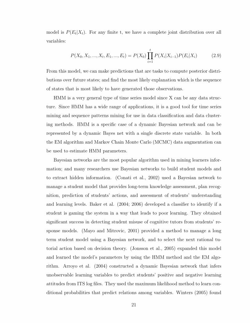
model is P (Et|Xt). For any finite t, we have a complete joint distribution over all
variables:
P (X0, X1, ..., Xt, E1, ..., Et) = P (X0)t∏i=1
P (Xi|Xi−1)P (Ei|Xi) (2.9)
From this model, we can make predictions that are tasks to compute posterior distri-
butions over future states; and find the most likely explanation which is the sequence
of states that is most likely to have generated those observations.
HMM is a very general type of time series model since X can be any data struc-
ture. Since HMM has a wide range of applications, it is a good tool for time series
mining and sequence patterns mining for use in data classification and data cluster-
ing methods. HMM is a specific case of a dynamic Bayesian network and can be
represented by a dynamic Bayes net with a single discrete state variable. In both
the EM algorithm and Markov Chain Monte Carlo (MCMC) data augmentation can
be used to estimate HMM parameters.
Bayesian networks are the most popular algorithm used in mining learners infor-
mation; and many researchers use Bayesian networks to build student models and
to extract hidden information. (Conati et al., 2002) used a Bayesian network to
manage a student model that provides long-term knowledge assessment, plan recog-
nition, prediction of students’ actions, and assessment of students’ understanding
and learning levels. Baker et al. (2004; 2006) developed a classifier to identify if a
student is gaming the system in a way that leads to poor learning. They obtained
significant success in detecting student misuse of cognitive tutors from students’ re-
sponse models. (Mayo and Mitrovic, 2001) provided a method to manage a long
term student model using a Bayesian network, and to select the next rational tu-
torial action based on decision theory. (Jonsson et al., 2005) expanded this model
and learned the model’s parameters by using the HMM method and the EM algo-
rithm. Arroyo et al. (2004) constructed a dynamic Bayesian network that infers
unobservable learning variables to predict students’ positive and negative learning
attitudes from ITS log files. They used the maximum likelihood method to learn con-
ditional probabilities that predict relations among variables. Winters (2005) found
21

the fundamental topic of a course and the proficiencies of each student by using col-
laborative filtering techniques such as non-negative matrix factorization, sigmoidal
factorization, and common-factor analysis. Using dynamic Bayesian network, Gong
et al.(2009) create a Knowledge Tracing model to make inferences about students’
knowledge and learning based on self-discipline. He found that high self-discipline
students had significantly higher initial knowledge. Using Markov Decision Process
technique, Stamper and Barnes(2009) promise a domain-independent use of data
mining method to automatically generate adaptive hints in an intelligent tutor sys-
tem. Based on the usage data and marks information, Romero et al.(2008) compared
different data mining methods to classify students, and found the classifier model
appropriate for educational use with both accuracy and comprehension. Bayesian
graphical models are commonly used in building student models. Desmarais et al.
(2008) designed a Naive Bayes Framework to explore the heuristic selection lead-
ing to better performance. Using data-driven modelling, Mavrikis (2008) compared
Bayesian network, decision trees and logistic regression methods to reveal the possi-
ble educational consequences.
2.3.5 Clustering
Clustering is a process of grouping data into distinct clusters (groups, categories, or
subsets) based on similarity among data. There is no universally accepted definition
of clustering. (Everitt et al., 2001) Most researchers describe a cluster by considering
the internal homogeneity and external separation (Hansen and Jaumard, 1997) for
example features of objects are similar to each other in the same cluster, while
features of objects are not similar when they are in different clusters. Three necessary
steps in implementing clustering algorithms are: the representation of data, the
definition of proximity among data, and applying clustering methods. The first
step obtains features or attributes to appropriately represent raw data. The second
step chooses a measurement to judge the similarity between two pieces of data such
as Euclidean distance between two data points, or Mahalonobis distance. Both
the similarity and dissimilarity should be examinable in a clear and meaningful
22

way (Xu and Wunsch, 2005). When data becomes more complex such as in trees
or sequences, determining similarity or dissimilarity becomes more difficult. Since
clustering algorithms are highly data dependent, the choice of a measurement for
similarity has a profound impact on clustering quality.
Here are two simple mathematical descriptions of two typical types of clustering.
(Xu and Wunsch, 2005; Hansen and Jaumard, 1997)
Given a set of input X = x1, ..., xj, ..., xN , where xj = (xj1, xj2, ..., xjd)T ∈ Rd
and each measure xji is said to be a attribute.
• Partitional clustering seeks a K partition of X, C = C1, ..., Ck(K ≤ N), such
that
1. Ci 6= φ, i = 1, ..., k;
2.⊔Ki=1Ci = X;
3. Ci⋂Cj = φ, i, j = 1, ..., K and i¬j.
• Hierarchical clustering attempts to construct a tree like nested structure of X,
H = H1, H2, ..., HQ(Q ≤ N), such that Ci ∈ Hm, Cj ⊂ Hl, and m limplyCi ∈
CjorCi⋂Cj = φ for all i, j 6= i,m, l = 1, ..., Q.
For clustering algorithms, there are four basic steps in the clustering procedure.
These steps are closely related to each other and affect the derived clusters. (Xu and
Wunsch, 2005)
• Feature selection: Feature selection chooses distinguishing features from a set
of candidate features or transforms to new and useful features from original
ones. It should be used to reduce noise, to be easy to select and interpret.
• Clustering algorithm selection: The selection of clustering algorithm is essen-
tially the selection of a proper proximity measure. The proximity measure
directly impacts on the formation of the resulting clusters. The partition of
clusters is an optimization problem once the proximity measure is determined.
However, there is no clustering algorithm that can be universally used to solve
23
all problems (Kleinberg, 2002). Therefore, it is very important to select an
appropriate clustering strategy to solve the problem properly.
• Clustering validation: The different algorithms usually have different clusters.
Therefore, it is necessary to use effective evaluation criteria to provide a certain
degree of confidence for resulting clusters from selected clustering algorithms.
Usually, there are three types of testing criteria: external indices, internal
indices, and relative indices and they are defined from three clustering struc-
tures, known as partitional clustering, hierarchical clustering, and individual
clustering. (Jain and Dubes, 1988)
• Results interpretation: The final purpose of clustering is to provide meaning-
ful insights to solve a problem so that the partition needs to be interpreted
carefully.
Clustering Algorithm Categories
Traditionally, accepted clustering algorithms are classified as hierarchical clustering
or partitional clustering based on the properties of generated clusters. (Xu and
Wunsch, 2005) In recent years, there are new categories of clustering algorithms
based on techniques, theories and applications. The following is a mixture of these
categorizations. (Xu and Wunsch, 2005)
• Hierarchical clustering
– Agglomerative: single linkage, complete linkage, median linkage, centroid
linkage...
– Divisive: divisive analysis, monotheistic analysis...
• Squared error-based (Vector quantization): K-means, genetic K-means algo-
rithm...
• Mixture density-based: expectation-maximization, Gaussian mixture density
decomposition...
24

• Graph theory-based: highly connected subgraphs...
• Fuzzy: Fuzzy c-means, fuzzy c-shells...
• Neural network-based: learning vector quantization...
• Kernel-based: support vector clustering, kernel k-means...
• Sequence data: sequence similarity...
• Large-scale data: CURE...
• High dimensional data: PCA...
The techniques-based clustering algorithms such as graph based, neural network
based and kernel based clustering algorithms can be used both in partition and hier-
archical clusterings. We will briefly discuss the k-means clustering and expectation-
maximization clustering in the following sections.
Distance and Similarity Measures
The first important issue of clustering algorithms is how to measure the distance or
the similarity between two objects, or a pair of clusters in order to determine the
closeness. In mathematics, a distance or similarity function on a data set is defined
to satisfy the following conditions:
1. Symmetry: D(xi, xj) = D(xj, xi);
2. Positivity: D(xi, xj) ≥ 0 for all xi and xj;
3. Triangle inequality: D(xi, xj) ≤ D(xi, xk) +D(xk, xj) for all xi, xj and xk;
4. Reflexivity: D(xi, xj) = 0 iff xi = xj;
There are some typical measures which can be used in determining the distance
or the similarity.
The Euclidean distance is the most commonly used metric to measure the dis-
tance between a pair of elements or a pair of clusters such as in hierarchical linkage
25

Minkowski distance Dij = (∑d
l=1 | xil − xjl |1/n)n
Euclidean distance Dij = (∑d
l=1 | xil − xjl |1/2)2
City-block distance Dij =∑d
l=1 | xil − xjl |
Sup distance Dij = max1≤l≤d | xil − xjl |
Pearson correlation Dij = (1− rij)/2
Table 2.2: Typical measures of distances
clustering, squared error-based k-means clustering and mixture densities EM clus-
tering. (Han and Kamber, 2001) The Minkowski distance, City-block distance and
Sup distance are normally used in fuzzy clustering algorithms.
Partitional method
A Partitional method divides a dataset into k clusters. K-means and k-medians are
two popular square-error based hard partitional clustering methods that are iterative
algorithms to minimize the least square error criteria. The mode-seeking method
and grid-based methods are density based clustering methods that regard clusters as
dense regions of data or grid of data structure in the data space separated by regions
of relatively low density. Graph based methods transform clustering problems into
a combinational optimization problem that can be solved by using graph algorithms
and related heuristics such as cutting the longest edge of the minimum spanning tree
to create clusters of nodes. Mixture distribution models assume data are generated
based on probabilities that are dependent on certain distributions such as Gaussian
distribution. A fuzzy c-means algorithm assigns a degree of certainty that specific
data belong to certain clusters.
Hierarchical method
A hierarchical method creates a hierarchical decomposition of data and uses methods
such as the following. The agglomerative (bottom-up) approach starts with each data
element forming a separate group and then merges groups that are closest according
to some distance measure (e.g. single link and complete link methods). The divisive
26

approach starts with all data in the same cluster and then splits into smaller clusters
in each iteration according to some measures.
Ayers et al. (Ayers et al., 2009) compare the performance of the three estimates
of student skill knowledge under a variety of clustering methods including hierarchi-
cal agglomerative clustering, K-means clustering and model-based clustering using
simulated data with varying levels of missing values. To support teacher’s reflec-
tion and adaptation in intelligent tutoring systems, Ben-Naim et al. (2009) used
a solution trace graph method to help teachers understand students’ behaviours in
an adaptive tutorial by post-analysis of the systems’ data-log. In constructing an
intelligent tutoring system, finding the level of learners’ background knowledge is
an unresolved problem. Antunes (2008) used sequential pattern mining methods to
automatically acquire that knowledge. Baker and Carvalho (2008) compared hier-
archical classifiers and non-hierarchical classifiers to identify exactly when a special
behaviour occurs in the gaming detector systems.
K-means Clustering Algorithm
The k-means clustering algorithm is the best-known squared error-based algorithm
which minimizes the squared error while partitioning elements into k clusters. The
basic steps of k-means clustering algorithm are:
1. Initialize k clusters randomly or based on some prior knowledge. Calculate the
cluster properties M = [m1, ...,mk]
2. Assign each element into the nearest cluster Ci based on the distance between
elements and clusters
3. Recalculate the cluster properties based on the current partitioning
4. Repeat steps 2 and 3 until convergence is reached
The k-means clustering algorithm is very simple and works well in many practical
problems. It is well studied and can be easily implemented in many applications.
Obviously, the k-means clustering algorithm also has some disadvantages and lots of
27

variants of k-means clustering algorithms have been developed in order to overcome
its drawbacks. The main drawbacks include lack of a universal method to identify
the initial partitions and the number of clusters, lack of a guarantee to converge to
a global optimum, and sensitivity to outliers and noise.
Mixture Gaussian Model
The mixture Gaussian clustering model is a classic statistical method with an as-
sumption that data is generated based on a mixture of k components that have
multivariate Gaussian distributions.
Expectation Maximization is the most popular method of mixture densities-
based clustering. From the probabilistic view, clustering presumes that the data
objects are generated from a mixture distribution such that this distribution has k
components and each component is a distribution in its own right. If the distributions
are known, finding the clusters of a given data set is equivalent to estimating the
parameters of underlying models. Let the random variable C denote the cluster
components, with value 1,...,k; then, the mixture distribution (probability density)
is defined as
p(x|θ) =k∑i=1
p(x|Ci, θi)P (Ci) (2.10)
Here, θ is the parameter vector, P (Ci) is the prior probability and∑k
i=1 P (Ci) = 1,
and p(x|Ci, θi) is the component density. The posterior probability for assigning a
data point into a cluster can be calculated with Bayes’s theorem while the parameter
vector θ is decided. Multivariate Gaussian is the natural choice to construct the
mixture density for continuous data.
The maximum likelihood estimation is an important statistical method to esti-
mate parameters because it maximizes the probability of generating all the observa-
tions by giving the joint density function in logarithm form
ι(θ) =N∑j=1
lnp(xi|θ) (2.11)
The best estimate can be achieved by solving the log-likelihood equations.
28

The expectation maximization algorithm is the most effective method to approxi-
mate the maximum likelihood since the analytical solution of the likelihood equation
cannot be obtained in most circumstances. The standard expectation maximiza-
tion algorithm calculates a series of parameter estimates θ0, θ1, ..., θT , through the
following steps:
1. initialize θ0 and set t = 0
2. e-step: compute the expectation of the log-likelihood
Q(θ, θt) = E[logp(C|θ)|X, θt];
3. m-step: select a new parameter estimate that maximizes the Q-function, θt+1 =
argmaxθ(θ, θt);
4. increase t = t+1; repeat steps 2 - 3 until the convergence condition is satisfied.
In ITS systems, following work that identifies which items produce the most
learning, Pardos and Heffernan (2009) proposed a Bayesian method using similar
permutation analysis techniques to determine if item learning is context sensitive
and if so which orderings produce the most learning. Nugent et al. (2009) has im-
plemented an approach to estimate each student’s individual skill knowledge. The
method has adapted several clustering algorithms including hierarchical agglomer-
ative clustering, k-means clustering, and model-based clustering to introduce an
automatic subspace method which first identifies skills on which students are well-
separated prior to clustering smaller subspace. Using data mining techniques, Sacin
et al. (2009) propose the use of a recommendation system to help students take
academic decisions based on available information.
2.3.6 Regression
Regression problems involve the prediction of continuous outcomes. Linear regres-
sion is the simplest form of regression in which data is modelled using a straight
line. The coefficients of linear regression can be solved by using the least squares
29

method. Multiple regression is an extension of linear regression that involves more
than one predictor variable. Nonlinear regression such as polynomial regression can
be transformed to linear regression.
The common regression methods used in data mining are: linear regression,
polynomial regression, robust regression, cascade correlation, radial basis functions
(RBFs), regression trees, multilinear interpolation, group methods data handling
(GMDH), and multivariate adaptive regression splines (MARS).
Regression methods were used by Feng (2005) to predict learners’ knowledge
levels from error sources. To determine the relative efficacy of different instructional
strategies, Feng et al. (2009) used learning decomposition, an educational data
mining technique, and logistic regression methods to determine how much learning
is caused by different methods of teaching the same skill.
2.3.7 Support Vector Machines
Support Vector Machines (SVMs, also called kernel machines) use efficient training
algorithms and can represent complex and/or nonlinear functions. The idea of SVMs
is that data will always be linearly separable if they can be mapped into a space with
sufficiently high dimensions. Various kernel functions can be used to map data into
some corresponding feature spaces, which have support vectors to hold separating
planes.
Support vector machines were used by Joachims (2001) in building learning mod-
els of text classification. A method called ”power law of learning” was used by
Koedinger and Mathan (2004) in determining whether students can flexibly use
knowledge learned from a course. Makrehchi and Kamel (2005) combined together
a vector space machine, weight regression, and similarity measures to build a social
network in a small community.
Other data mining algorithms include instance-based learning (such as the
nearest-neighbor model and the kernel model), neural networks, and distributed
data mining methods.
30

Chen et al. (2004) proposed an approach to automatically construct an e-
textbook via web content mining. They used a ranking strategy to evaluate the
web pages and extract concept features from web contents. To extract from the
discussion forum with viewable and useful information for instructors, Dringus et
al. (2005) proposed a strategy using text mining to assess an asynchronous discus-
sion forum. Their experiment shows that using text mining techniques in the query
process could improve the instructor’s ability to evaluate the progress of a threaded
discussion. Hershkovitz and Nachmias (2009) investigate the consistency of students’
behaviours regarding their pace of actions over sessions within an online course. The
results suggest that pace is something not consistent. Web mining methods also were
used by Merceron and Yacef (2003) to improve learning and teaching. By combining
data mining and text mining methods together, Nagata et al. (2009) proposes a
novel method for recommending books to pupils based on only local histories with
an accuracy 60% performance. Rai et al. (2009) propose a technique that directly
produces parameters to improve the understanding students’ knowledge. Ritter et
al. (2009) find a way to reducing the knowledge tracing space and parameters to
improve great efficiency gains in interpreting specific learning and performance from
students’ models. Using heuristic classification model, Hubscher and Puntambekar
(2008) described a method to integrate the knowledge discovered with data mining
techniques, pedagogical knowledge and linguistic knowledge together.
As presented in previous sections, data mining techniques are promising for
automatically creating learner models because they try to capture meaningful pat-
terns that have been found in the interactive data. Learner models are implicitly
and explicitly created in educational data mining applications, especially applica-
tions oriented toward learners in which the knowledge of learners must be captured
in order to create a learning environment that can be individualized to each learner.
In the rest of the thesis we explore the general questions of how to create learner
models automatically from observations of learner behaviours. In particular we pro-
pose an approach where EDM techniques allow us to observe stable metrics from
31

learner behaviours that can be the basis for metrics and measurements that can be
applied by an online system to understand learners as they interact with an educa-
tional system.
32

Chapter 3
Dynamically Mining Learners’
Characteristics
“The ecological approach shows promise not only to allow information about learn-
ers’ actual interactions with learning objects to be naturally captured but also to allow
it to be used in a multitude of ways to support learners and teachers in achieving their
task.” (McCalla, 2004)
3.1 Motivation
Unlike in traditional classrooms in which teachers observe learners’ performances
through direct observation and communication, and then adapt their personal strate-
gies to improve learners’ learning processes, most web-based e-learning systems try
to add the ability to adjust learning contexts and contents to improve individuals’
learning processes. Adaptive and intelligent systems are being built to investigate
the personalization of learning contexts. To provide personalized contexts, an adap-
tive and intelligent e-learning system tries to meet the individual learner’s needs by
understanding what the learner’s expectations are. There are two methods to gather
the learners’ characteristics, preferences and past experiences – the static method
which uses surveys, questionnaires, existing documents and historical records to col-
lection information, and the dynamic method which instead learns information about
learners from data collected in real time. The core aspect of the dynamic method
is the continual reuse of data, so that the knowledge learned from observations will
continue to be applied to the system in order to strengthen and enrich its abilities
33

to encourage better performances of learners.
Our work is done in the context of a real system, iHelp, where large amounts of
usage data have been collected from the interactions among instructors and learners.
The data collected from the iHelp system is organized into a database at a fine-
grained level. This data is a combination of static information about learners and
learning objects, as well as dynamic data coming from learner, instructor and system
activities. Our basic research questions are: what kinds of learning patterns can
we mine from the iHelp data set, and how we can use these patterns to facilitate
pedagogical purposes. At the beginning, we tried to apply data mining techniques,
such as classification and association rules mining, directly to the raw data sets. In
this way, we created many results. The main issue of this method is that we cannot
identify prominent learning patterns and irrelevant patterns from these results.
We needed to reason with this usage data at higher levels of granularity. Thus,
in this chapter, we introduce a six layer model which mines dynamic learner models.
The six layers include raw data layer, fact data layer, data mining layer, measure-
ments layer, metric layer and application layer. The key components in this model
are the metrics and measurement layers, which provide an efficient way to represent
learners’ characteristics and knowledge, and the data mining layer, which provides
the tools to retrieve information.
The details of this chapter include how to collect data, why it is called purposes
based method, why it is a six layer model, and how to implement in the real learning
environment.
3.2 Data Collection
Our system focuses on the reuse of information collected by e-learning systems such
as the iHelp system. Like other e-learning systems, iHelp records all information
about interaction among learners, instructors, and the system into a database at a
fine-grained level. Our interests are in the following three kinds of data:
• Data about learners: consists of personal information, knowledge structures,
34
intentions, activity status, goals, previous experience and social activities.
• Data about learning objects: consists of knowledge contents, organized struc-
tures (which are a combination of text, graphics, web pages, reference links, and
multimedia documents), pre-defined metadata, qualities, ratings and interest
levels.
• Data about interactions: consists of observed attributes such as dwell time,
following links, depth of navigation, sequence of navigation, recurring events
like question and/or answer postings, chattiness and qualities of interactive
events.
It is necessary to transform and filter raw data such that we can construct rela-
tions between learners and learning objects, and find information about interactions
based on such relations.
3.2.1 Raw Data
We can directly use this data collection as the starting point for our analysis. The
iHelp system consists of the components in Table 3.1; we briefly describe potential
data collected from each component.
• iHelp LCMS: From this database scheme, we can find system information,
management information, a learner’s personal information although the learn-
ers remain anonymous by hiding their real identifications, course information,
course id, learning object/module information, etc. The instructors and admin-
istrators collect and enter into the system to initialize the course management
module.
• iHelp Discussion: From the iHelp asynchronous discussion forum, we can col-
lect information such as login and logout events, messages read and written,
contents of messages, messages threads, etc. This information records how
learners are involved in the discussion activities.
35

• iHelp Chat: From the iHelp synchronous chat room, we can collect enter chat
channel and leave chat channel events, messages read and written, contents of
messages, etc. This information records how learners are involved in the chat
room activities.
• iHelp Course: From this distance learning component of iHelp, we can collect
login and logout events, contexts of web pages, relationships of web pages, nav-
igation sequences, dwell time on web pages, quiz questions, marks of quizzes,
etc. This information records how learners browse course web sites, and do
on-line quizzes.
iHelp Share and iHelp Lecture will not be used in our analysis.
login/logout dwelltime messages events sequence marks static
iHelp LCMS Yes Yes No Yes Yes No Yes
iHelp Discussion Yes Yes Yes Yes Yes No No
iHelp Chat Yes Yes Yes No Yes No No
iHelp Course Yes Yes No Yes Yes Yes No
iHelp Share Yes N/A Yes Yes N/A Yes Yes
iHelp Lecture N/A Yes N/A N/A No No No
Table 3.1: Potential data in each iHelp component
3.2.2 Fact Data
The raw data in the iHelp database mostly are events recorded in chronological order.
For some kinds of events like dwell time and navigation times, we need to combine
them in order to correctly describe learners’ behaviours. In our analysis, we call this
combined data “fact data” as it reflects real characteristics of learners. Not only
does fact data represent characteristics of learners, but it also can represent features
of learning objects. In Table 3.2, we see some examples of data types and the origin
of each factor associated with learners.
36

Fact Data Name Calculation Original Description
navigatetimes Summation iHelp lcms, Course measures how many times a
learner navigates web pages
contentnum Summation
of Distinct
Events
iHelp Course measures how many non-
repeat web pages a learner has
navigated so far
readingtimes Summation
Events
iHelp Discussion measures how many times a
learner reads posting mes-
sages of a specific topic
chatnum Summation
of Distinct
Events
iHelp Chat measures how many channels
a learner involved
Table 3.2: Some fact data and their original sources
Here are database scripts to elicit fact data navigatetimes, contentnum, and dwell-
time from raw data in the iHelp database.
1. First script: Calculate dwell time for each navigation in current session
CREATE OR REPLACE VIEW n dwell time (userid, contentid, exit time, en-
ter time, dwelltime) AS
SELECT userid, contentid, exit time, enter time, IF (exit time=’0000-00-00 00:00:00’,
0, TIME TO SEC (TIMEDIFF (exit time, enter time))) AS dwelltime
FROM lcms. user navigation n
WHERE courseid = (SELECT courseid FROM n init)
AND userid IN (SELECT userid FROM n all learners)
2. Second script: Filter out the navigating times, number of contentid, dwell time
CREATE TABLE r sum contents
SELECT d.userid, COUNT (d.contentid) AS navigatetimes, COUNT (DISTINCT
d.contentid) AS contentnum, SUM(d.dwelltime) AS dwelltime
FROM (SELECT * FROM n dwell time) AS d
37

GROUP BY d.userid
In this way we initially create a repository of fact data by transforming raw
data. Throughout this conversion process, we collect useful raw data, and throw out
unimportant details. Filtering is a classical technique that finds a few relevant items
in a large pool of items, and is generally used in adaptive and intelligent systems.
3.3 Purpose-Based Methods
The key aspect of the ecological approach is the purpose-based use of the information
associated with the content, to achieve a particular goal (McCalla, 2004). The
pedagogical purpose determines what kind of characteristics of learners or learning
objects have to be known to support this purpose, and what kind of information
should be captured from e-learning systems to identify these specific characteristics
of learners or learning objects.
This top-down method facilitates the identification of requirements and con-
straints for each particular pedagogical purpose at a high level before considering
low level details, and clarifies which are candidates for data mining and machine
learning techniques. This is in contrast to the bottom-up approach which requires
us to find patterns from the raw data regardless of how or where these patterns are
useful. It is extremely difficult to find useful and meaningful patterns directly from
low level data.
3.3.1 Pedagogical Purposes
From e-learning systems such as iHelp, we know there are many pedagogical purposes
which could be fulfilled to understand learners better, to provide personalized content
or services. Both recommending content and finding peer helpers are such purposes.
Recommending relevant content for a particular user requires us to compare this user
to other users based on some important characteristics and experiences, and then
to evaluate contents based on similar users’ assessments (Tang and McCalla, 2005).
38

Finding peer helpers for answering a specific question requires us to evaluate users
based on the domain of the problem to find potential expert candidates, and then
to recommend the best helper by comparing users based on their characteristics and
experiences. Pedagogical purposes have various forms. McCalla (2004) highlights
some possible pedagogical purposes:
• recommending relevant learning objects to meet a learner’s specific needs
• recommending learning patterns to improve a learner’s skills
• finding information related to a particular learning object
• finding a peer helper to provide face-to-face help for a specific problem
• evaluating the effectiveness of learning objects
• finding similarities between learners
• determining semantic relationships between learning objects
The common points of these pedagogical purposes are that the purposes deter-
mine what characteristics and experiences of learners or learning objects are relevant
and necessary to fulfil the purpose. So the purposes determine what information is
relevant, where to look for such information, and how to combine the information
together to support characteristics and experiences of learners and learning objects.
3.3.2 Methods Based on Purposes
In e-learning systems, learning content could be web pages, content of messages,
research papers, courses of study, quizzes or tests, text books, and multimedia doc-
uments, etc. The term learning object may refer to any of these possibilities. The
learner model refers to the characteristics, preferences and experiences of a learner.
The term “metric” represents an aspect of learners’ characteristics, preferences, and
experiences the in the learner model. Metrics could be learners’ activities, learners’
social connections and learners’ learning styles, etc.
39

We need a way to describe the relationships among information, characteristics of
learners, and purposes. The purposes require and determine the relevant character-
istics of learners. The information about learners, learning objects and interactions
imply the possible characteristics of learners. Transformation from raw data into
fact data does not change the meaning of the information. Characteristics, prefer-
ences and experiences of learners are naturally represented by metrics in the learner
models. The purposes need to be implemented and achieved by applications. The
purpose determines the relevant and necessary learner models, and how the learner
model are be captured and retrieved from fact data. Data mining technique is a
nature way to use existing information to support pedagogical goals.
To further illuminate the methods based on purposes, we highlight some inter-
esting data fields (fact data), potential learning models (metrics), and some possible
applications (purposes) in Figure 3.1. On the left-most rows are the attribute data
fields; on the top columns are metrics; and on the right-most rows are purposes. In
each cell, a letter ”Y” implies that a learner model could use the particular attribute;
a grey colour means such a learner model is essential for the correspondent purpose.
For example, the activity level metric is derived from fact data such as login/logout,
dwell time, events associating with learners and learning objects, information from
discussion forums, information from chat room interactions, and quizzes events. The
purpose of recommending a peer helper can use metrics such as activity level, social
tendency, learning style, learning attitude, communication style, response tendency,
and knowledge tendency.
3.4 Dynamic Learner Model
From the above discussion, it is clear that there are relations among information,
learner model and applications. We can thus clearly foresee that information will be
reused to build up learner models, and furthermore to support new applications, as
in the ecological approach. This also is a dynamic process because we will count on
the data to be updated in real time before the computing procedure happens. Based
40

Figure 3.1: Relationships among purposes, metrics and attributes
41

Figure 3.2: Six layers model
on this analysis, we can create the model which will produce the dynamic learner
models.
3.4.1 Model
This model consists of six layers as Figure 3.2 shows. Each layer depends on the
layer below. Based on previous analysis, the top application layer consists of the ed-
ucational applications; the metric and measurement layers correspond to the learner
models; and the bottom raw data and fact data layers correspond to information.
The data mining layer represents the information retrieval procedure which dynam-
ically creates and supports the measurements in this model. Here, each metric is
composed by combining measurements of specific data relevance to it. As an ex-
ample, the activity level metric, is built out of measurements such as activity level
in reading discussion messages, activity level in browsing course materials, activity
level in the chat room, etc.
Metrics represent aspects in the learner model, characteristics, preferences and
experiences of learners. Metrics are at a level higher than measurements thus hiding
the details of where the information comes from. The measurements supply more
details to the metrics and can also be used individually to support the applications.
The measurements are the results of patterns found in the raw information that are
meaningful to the ultimate applications. The fact data are filtered and sorted from
42

raw data as described in the data collection section.
3.4.2 Layers
There are four transitions in the model as information is interpreted from the lowest
level raw data to serve the applications. Each transition is discussed below.
From Raw Data to Fact Data
Raw data is directly collected from an e-learning environment. The raw data includes
static information such as learners’ personal information and predefined preferences,
dynamic information such as login/logout events, messages, sequence events, etc.
We say the raw data are directly extracted from the e-learning system because they
are already available there. So any computation for recording these data must have
finished before we extract them.
Raw data is transformed to fact data about learners or learning objects. To obtain
the fact data, we filter and sort the raw data under various predefined constraints
and criteria. The common filtering conditions relate to the learners, the courses, the
learning objects, etc. An example is setting the length of interval of sequence data to
one or two hours; another is only counting messages from learners who are involved
in the same course, etc.
One issue is what kind of fact data we can get from the raw data. It really depends
on each particular e-learning system. We cannot create data without sources, but we
may provide new information by combining some raw data together, such as creating
frequency attributes. Usually learners must follow some routines in a closed learning
environment while an open learning environment do not restrict learners’ actions
such as iHelp system. Data coming from closed e-learning environments are more
likely to be interesting and of high density than data coming from open e-learning
environments. The other issue is that fact data requiring filtering and sorting raw
data may need large computations and may take a long time to finish. Because one
feature of many e-learning systems is that the volume of data increases slowly on a
daily basis, we have a chance to pre-compute fact data of this sort.
43

From Fact Data to Measurements
Fact data are transformed into measurements using data mining techniques. Unlike
fact data, measurements have clearly determined and meaningful definitions relevant
specifically to learning. In this way, we avoid judging and choosing the meaningful
and useful hidden patterns from the data mining results; instead we have to decide
which fact data should be used as the inputs. This is where purposes come in. The
hope is that experts, such as instructors, can figure out which fact data are relevant
to a measurement for the specific purposes of an application.
In general, both classification and clustering algorithms can be applied. If we
have defined the classes of measurements and have the training data, we would
choose classification and prediction data mining algorithms. Or if we do not have
the classes of measurements, we can apply clustering algorithms to group the learn-
ers or the learning objects into different clusters. How to choose the number of
clusters in clustering algorithms is always an issue; and the solution depends on the
domain of knowledge about the problem; and here this issue is solved by combining
expert opinions and the features of the particular measurement. For example, the
activities of learners can be grouped into four levels as dormant, passive, active and
hyperactive. Figure 3.3 shows data we used in a pilot study to be described later
in the thesis. Figure 3.4 and 3.5 shows how we can apply cluster and classification
algorithms to create different groups.
The measurements are the output of the fact data layer which either predicts the
classes of instances or detects a number of clusters to group the instances. Learners
can then be categorized appropriately as an instance of a class or as being in a
particular cluster. The measurements expect the metrics to reflect more details such
as for the activity metric: the activity level in browsing web pages, the activity level
in reading messages, the activity level in doing quizzes, etc. The measurements also
can focus on one aspect of the metrics such as restricting the learning style metric
to active or reflective learners, or to global learners or sequence learners etc.
The measurements are selected and determined as to whether the purposes re-
44

Figure 3.3: Fact data in the pilot study
quire them and whether the fact data support their calculation. Not all of the
measurements required by purposes can be computed from the fact data if we lack
appropriate raw data, or if we lack the knowledge of how to capture them.
From Measurements To Metrics
Metrics reflect general characteristics of learners that may be important to an appli-
cation. Each metric consists of several measurements. The metrics are abstractors
without explicit values, used to categorize the measurements which have actual dy-
namic assigned values. By analyzing various pedagogical purposes, we list some
potential metrics in Figure 3.1 that would be useful for a learning system. Some
metrics rely on measurements based on interaction and usage data. Four we have
explored are activity level, social tendency, learning style and knowledge tendency.
45

Figure 3.4: Clusters in the pilot study
The activity level metric measures learners’ activities in iHelp system. The social
tendency metric measures how learners connect with each other. The learning style
metric defines what kinds of learning style a learner may have. The knowledge ten-
dency metric measures learners’ possible knowledge about learning objects. Other
metrics may need richer information provided through other techniques such as text
mining. We have not expanded these in this thesis.
From Metrics To Applications
The applications are the adaptive tools and components which use the metrics and
measurements, to improve the ability and efficiency of the e-learning systems.
3.4.3 Dynamic Procedure
Modelling in this approach is a dynamic procedure because the computations will
apply on the data accumulated to the current time rather than referring to static
historical records. Whenever we need to compute the values of the measurements
and metrics, we can use data mining techniques to retrieve them from the data,
appropriately synchronized and updated. This dynamic procedure guarantees that
the metrics and measurements really reflect the current status of the learner models.
46

Figure 3.5: Classification in the pliot study
Since the system will collect more data as time passes, it is important to keep the
learner models synchronized with the system to reflect the contributions of new data.
It does not mean that historical records are not useful.
To dynamically compute the learner models, we must be concerned with efficiency
issues in doing real time computations. There are two general questions about the
computation time. Can we do the computation in reasonable time? And is there a
possibility to do pre-computation? The solutions depend on how complex the data
mining algorithms are, and the size, the length, the dimensions, and the scale of
data. We argue that for applying data mining algorithms in educational data, pre-
computation is often necessary to guarantee the key components can be computed
in a reasonable time. Since the data preparing and filtering step is a time consuming
task in data mining, this step is a good choice for pre-computation to speed up the
whole procedure. This corresponds especially to the raw data to fact data and fact
data to measurements transitions in our approach. Our experiments prove that the
proper pre-computation is necessary and can be managed. Since “reasonable time”
varies in the different situations, it is hard to find a universal solution.
47

3.5 Implementation of Dynamic Learner Modelling
To get first hand experience as to how this approach will work, we designed a pilot
study that created and evaluated selected metrics and measurements to estimate
dynamic learner models. To make things simple, we focused on the purpose of
finding peer helpers in order to select and evaluate some metrics which relate with
the usage data. Such metrics will give us insight as to the learners’ characteristics,
preferences and experiences. We will compare these automatically generated metrics
with experts’ opinions and learners’ self evaluations in our experimental analysis.
3.5.1 Selection of Raw Data and Fact Data
We use raw data extracted from the iHelp system (See Table 3.1). The fact data are
filtered and sorted from the raw data as shown in Table 3.3. Figure 3.6a shows how
to set up the filtering conditions to extract the measurement data.
Fact Data Name Computation Description
navigatetimes Sum measure how many times a learner browse web
pages
contentnum Count Distinct measure how many no repeat web pages a learner
browses so far
dwelltime Sum measure how long a learner spends on browsing
web pages
readingtimes Sum measure how many times a learner reads posting
messages
readpostingnum Count Distinct measure how many posting messages a learner has
read so far
totalmsg Sum measure how many messages a learner has written
so far
Continued on next page
48

Table 3.3 – continued from previous page
Fact Data Name Computation Description
replymsg Count measure how many messages are written to reply
other learners
newmsg Count measure how many messages are written as new
(non-reply) messages
replyfrequency Percentage measure a ratio of reply messages over total mes-
sages
replyscale Count Distinct measure how many topics a learner replies to
sentnum Sum measure how many sentences a learner writes
chatnum Count Distinct measure how many channels a learner involves
event Sum measure how many times a learner is active in a
channel
joined Count measure how many times a join event has hap-
pened so far
focused Count measure how many times a focus event has hap-
pened so far
scoretimes Sum measure how many times a learner completes
quizzes
scorescale Count Distinct measure how many quizzes a learner has completed
so far
scores Sum measure the sum of all quizzes’ marks for a learner
total Sum measure how many hours a learner spends so far
high Count measure how many hours a learner has high con-
centration based on a pre-defined threshold
middle Count measure how many hours a learner has middle con-
centration based on a pre-defined thresholds
Continued on next page
49

Table 3.3 – continued from previous page
Fact Data Name Computation Description
low Count measure how many hours a learner has low con-
centration based on a pre-defined thresholds
undefined Count measure how many hours a learner is on undefined
status
global Count measure how many times a learner has changed
events among web, read, write, chat, quiz
events Sum measure how many events happened for a learner
so far
focus Count measure how many times a learner is working on
the same context before changing events
unchange Count measure how many times a learner doesn’t change
context when events changed
userid Distinct alias name of learners
Table 3.3: The fact data
3.5.2 Selection of Data Mining Algorithms
As we do not have predefined classes for the measurements; we choose clustering
algorithms to divide the learners into different groups, and then assign a label to
each group. When preparing the data set we normalize the fact data into numeric
data sets which are filtered from the raw data. It is natural to use Euclidean distance
to measure distances between two numeric data sets. When we choose the clustering
algorithms, we thus consider only those algorithms that can use numeric data and
Euclidean distance. From the open source Weka (Witten and Frank, 2005) tools, we
select four algorithms that fulfil these constraints, and make some modifications to
match our situation.
50

(a) Setup parameters of sequence data (b) Setup clustering algorithms and labels
Figure 3.6: Setup parameters
The four clustering algorithms we used in this project are the expectation max-
imization clustering algorithm, simple k means clustering, x means clustering, and
the farthest first clustering algorithm. Expectation maximization (EM) is a density-
based algorithm that is favoured for incomplete data sets. Simple k-means, x-means
and farthest first are three varieties of square error-based clustering algorithms that
are simple and popular to use with Euclidean distance. To overcome overfitting and
local maximization issues, we set the cross validation parameter to ten to reduce the
chances that cluster centers fall into the local maximum. Considering that instruc-
tors normally categorize their students into limited groups, we predefine the number
of cluster centers for each algorithm in order to compare with human evaluation
results. Figure 3.6b shows how to set up the clustering algorithms and the clustering
labels for each metric in the Weka toolkit.
Define the Labels of Clusters
The clustering tools form cluster centers. Since this process does not sort and order
the cluster centers, we have to sort and assign a label to each cluster center based
on their proprieties. The formula used to compute the propriety of centers is:
Pi =n∑i=j
WjSort(Aij) (3.1)
51

Here, Pi is the propriety of the ith center; 0 < i < the number of cluster centers;
0 < j < the number of attributes; Wj is the weight of the jth attribute. High
propriety implies a strong tendency or possibility, and low propriety implies low
tendency or possibility with respect to the predefined labels of metrics. For instance,
assume the mining tool finds two clustering centers based on six attributes, the first
center has high propriety because it gets high values in four of six attributes so that
we assign the “high” label to it.
When we consider the weights of attribute data, we should avoid the case that
one attribute dominates the propriety if the weight of this attribute is large enough.
We used instructors’ input to decide the weights in our pilot studies.
3.5.3 Selection of Metrics and Measurements
We limit the metrics to those that can be ultimately computed from usage data
(other kinds of mining, such as text mining, are beyond our scope). Depending
on the available fact data, each metric consists of several measurements. Figure 3.7
shows how to add a new measurement, and how to change the attributes, the number
of clusters, and the weights of attributes. In our pilot system, we used four metrics:
the activity level, the social tendency, the learning style and the knowledge tendency.
We have a total of fifteen measurements from which the important characteristics of
these metrics are computed. We highlight these metrics and measurements in Table
3.4 because we will analyze the results for each measurement as well as the four
overall metrics.
The activity level metric reflects how often a learner is involved in various learning
processes such as browsing course materials, reading and writing messages, and doing
practical quizzes. The social tendency metric records the frequency and degree that
a learner communicates with other learners. The learning style metric reflects the
learning habits of a learner such that we can categorize a learner in terms of being
active or reflective, or a sequential or global learner. The knowledge tendency metric
implies a learner’s possibility of understanding the course materials, where a positive
values translates to a high possibility of understanding.
52
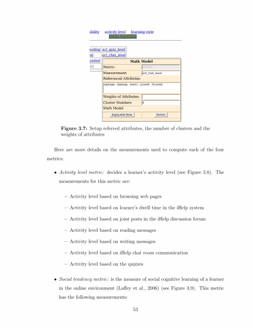
Figure 3.7: Setup referred attributes, the number of clusters and theweights of attributes
Here are more details on the measurements used to compute each of the four
metrics:
• Activity level metric: decides a learner’s activity level (see Figure 3.8). The
measurements for this metric are:
– Activity level based on browsing web pages
– Activity level based on learner’s dwell time in the iHelp system
– Activity level based on joint posts in the iHelp discussion forum
– Activity level based on reading messages
– Activity level based on writing messages
– Activity level based on iHelp chat room communication
– Activity level based on the quizzes
• Social tendency metric: is the measure of social cognitive learning of a learner
in the online environment (Laffey et al., 2006) (see Figure 3.9). This metric
has the following measurements:
53

metric measurement
user model
activity
context activity
dwell time activity
discussion activity
reading messages activity
writing messages activity
chat room activity
quiz activity
social tendency
navigation ability
presence ability
connectedness level
learning style
active or reflective learning
concentration level
sequential or global learning
knowledge tendencycontext level
quiz level
Table 3.4: Metrics and measurements in pilot study
– Social navigation: learning about and observing the actions of other learn-
ers
– Social presence: presence in asynchronous, text-based communications
(Short et al., 1976)
– Social connectedness: the level of connectedness to each other
• Learning style metric: is a learner’s learning style in the online environment
(see Figure 3.10). This metric includes measurements:
– Active or reflective learner: Active learners tend to learn something by
acting with it – discussing it or explaining it to others. Reflective learners
prefer to think about it quietly first.
54

Figure 3.8: Activity level metric
– Sequential or global learner: Sequential learners tend to gain understand-
ing in linear steps, with each step logically following the previous one.
Global learners tend to learn in large jumps, absorbing materials ran-
domly to look at the natural connections.
– Concentration: This measures the average time a learner spends on each
piece of course material
• Knowledge tendency metric: defines a learner’s attitude in the learning process
(see Figure 3.11). Two measurements are:
– Knowledge tendency based on learning course materials
– Knowledge tendency based on doing practical quizzes
Figure 3.12 shows the process of computing one measurement which includes the
cluster centers information, the distribution of the learner instances, and the labels
assigned to each individual learner. A learner’s dynamic learner model is presented
in Figure 3.13 which includes all computing results of the measurements and metrics.
Figure 3.14 shows the results of one metric for all learners.
55

Figure 3.9: Social tendency metric
Based on the selected metrics and measurements, we ran several experiments to
compare our data mining approach with human evaluations in order to prove the
dynamic learner model is a useful way to represent the characteristics, preferences
and experiences of learners. These experiments are described and discussed in the
next chapter.
56

Figure 3.10: Learning style metric
Figure 3.11: Knowledge tendency metric
57

Figure 3.12: Computing one measurement
58

Figure 3.13: Dynamic learner model of a learner
59

Figure 3.14: Computing one metric
60

Chapter 4
Analyzing the Metrics and Measurements
4.1 Introduction
We designed two experiments to evaluate the six layer model: one is an expert
evaluation and the other is a learner self evaluation. Using data from the iHelp
system, we compared our data mining results with human evaluation results. Then
we analyzed the advantages and disadvantages of our approach.
The data used in the expert experiment was collected from the Cmpt 100 online
course in term 1 of 2006 with 32 students using the iHelp system. The data used in
the learner self evaluation was collected from the iHelp usage data in the Cmpt 100
online courses in term 1 of 2007 and in term 2 of 2008. There were 50 students in
two classes, but only 14 students who did the self evaluations.
In the expert experiment, experts were required to evaluate each student’s be-
haviours in terms of four metrics and 19 measurements 1 through their examinations
of the iHelp usage data. The metrics are activity level metric, social tendency metric,
learning style metric, and knowledge tendency metric with particular measurements
associated with each metric. The average time an expert spent was about six to eight
hours. In short this experiment asked the human experts to evaluate the students
on the same metrics and measurements as the system did.
In the learner self evaluation experiment, we designed a questionnaire to col-
lect information from students that provided an alternative way of generating the
measurements of three metrics: social tendency metric, learning style metric, and
115 measurements and 4 totals
61

knowledge tendency metric.
From the two experiments’ results, we learned that some measurements are useful
in building just in time learner models; some only show promise to be headed in that
directions; and some don’t seem to be well supported at all. The expert experiment
shows more positive results than the self evaluation experiment. Overall, we think
that just in time computation of learner models shows promise to allow a system to
track change in students’ capabilities during the learning process.
4.2 Methods of Analysis
We use a confusion matrix to visualize and compare results, and analyze accuracy
and inter-rater reliability.
4.2.1 Confusion Matrix
A confusion matrix is a visualization tool, a table, used in data mining and artificial
intelligence systems. Columns of the matrix represent the instances of predicated
results or tested results, while rows of the matrix represent the instances of actual
results or true results. The diagonal elements represent matched compounds while
the off-diagonal elements represent misclassified compounds.
Figure 4.1: A confusion matrix
• Accuracy
For binary problem cases, in which the outcomes are labelled either as positive
or negative, we can easily calculate statistical characteristics such as accuracy,
precision, recall, fall out and F-measures. For problems in which the outcomes
62

are more than two states, we can only extend accuracy easily. In our study, we
only calculate accuracy since we have multiple outcomes in all cases.
Accuracy(AC) =
n∑k=1
nkk
n∑i=1
n∑j=1
nij
(4.1)
where nij is an element of the confusion matrix.
4.2.2 Inter-rater reliability
To test the evaluation quality, we need to calculate the reliability. Strong reliability
is important if we are to have a dependable measure in our user models. Generally,
reliability has four types: inter-rater reliability, test-retest reliability, parallel-forms
reliability, and internal consistency reliability. (Hogan et al., 2000) The inter-rater
reliability is to be used to assess the difference between raters. The test-retest relia-
bility is to be used to assess a measure from one time to another. The parallel-forms
reliability is to be used to assess the consistency of two tests from the same content
domain. The internal consistency reliability is to be used to assess the consistency
of results across times within one test. We only used the inter-rater and internal
consistency reliabilities in our study.
In comparing the data mining results and the expert evaluations results, we used
kappa coefficient to measure the inter-rater reliability. Since our confusion matrices
are multiple dimensional matrices rather than a binary matrix, it is hard to apply
other popular methods such as intraclass correlation (ICC).
• Cohen’s kappa (Inter-rater reliability measure)
Cohen’s kappa coefficient measures the agreement between two raters on classi-
fying some items into predefined categories. The definition of kappa coefficient
k is:
k =
nq∑
k=1
nkk −q∑
k=1
(q∑i=1
nkiq∑j=1
njk)
n2 −q∑
k=1
(q∑i=1
nkiq∑j=1
njk)
(4.2)
63

• Correlation coefficient (Internal Consistency Measure)
Correlation coefficient is another statistical tool to measure pairwise correlation
among two variables. It measures the tendency of the variables to increase or
decrease together. It is better to demonstrate that the data mining results
share a very similar curve tendency with the human expert’s results, that they
have a linear relationship.
rxy =
∑(xi − y)(yi − y)
(n− 1)sxsy(4.3)
4.3 Experment I – Expert Evaluation
4.3.1 Experiment Information
Summary of Raw Data
We chose to analyze iHelp data from one online class:
• Class Name: CMPT 100 online
• Term: 1
• Year: 2006 - 2007
• Size: 32 students
records total average per learner maximal per learner
navigating web pages 46109 1441 5077
dwell time (in hours) 1318.93 41.22 116.16
discussion forum messages 177 5.5 33
reading messages 6655 208 894
chat room messages 1479 46 239
doing quizzes 366 12 39
Table 4.1: Summary of the raw data
64

Figure 4.2: Result of one measurement
Data Mining Results
Just in time learner models (such as the one shown in Figure 4.4) based on metrics
and measurements extracted from learner behaviour on iHelp are the models used
in comparison to similar models built by the experts.
Figure 4.2 shows the computing results of one measurement with the information
of cluster centers and distribution of population. Figure 4.3 shows the computing
65

Figure 4.3: Results of one metric
66

Figure 4.4: Result of one learner
67

results of one metric for all learners while cluster labels have been assigned to each
measurement cluster groups. Figure 4.4 shows the results for one learner.
4.3.2 Expert Evaluation
In the expert evaluation, we ask experts to make their own judgements for each
learner on each measurement of each metric. There are four metrics and fifteen
measurements. The total records of each expert are: (4 + 15) * 32 = 608. Each
expert spent approximately six to eight hours to take part in this evaluations during
three days. A web server provides details about each learners and descriptions about
information. Experts used a web browser to compare learners’ information and to
make judgement with confidence parameters. Figure 4.5 shows an example of an
expert’s evaluation of a learner. Results are directly stored into the database of the
server. Experts could go backward to change, modify, and correct their evaluation
results to get more precise comparison; and we keep tracking all changes in the
database.
We predefine classification labels for each measurement and each metric. The
classification labels are the same as the labels used in the dynamic clustering pro-
cedure. Experts assigned a label from this set for each record based on their own
judgement. Experts also assigned each record a confidence level which we can use
as a weighting factor in our later analysis of the evaluation results.
Four experts, who are instructors or have teaching experience, did the evaluation.
Two of them finished all required evaluations, and other two only partially finished
evaluations because it will take too long to evaluate all learners. Final analysis in this
thesis is based only on results of the two experts who finished the total evaluations
(to maximize consistency and reliability).
For each measurement, we wanted to compare the evaluations (for all 32 students)
of the experts to the system. For this purpose we used a confusion metric, such as
the one for “navigating contexts” in Figure 4.1. The left upper cell is the name of the
measurement. The columns of the confusion matrix are system results; and the rows
of the confusion matrix are human evaluation results. For example, the cell value
68

Figure 4.5: Human evaluation working page example
2 (in the row 2 and the column 1) means that the system assigned passive to two
students and the expert assigned dormant to them. The entries in main diagonal of a
confusion matrix are numbers of human results exactly matching system results. The
entries outside of main diagonal are numbers of human results mismatching system
results. The right-most column and the lowest row summarize each classification. In
Figure 4.1, entries on the diagonal are the number of expert results that agree with
system results; entries above the diagonal are the number of expert results that give
high evaluations than the system results; entries below the diagonal are the number
of expert results that give lower evaluation than the system results; entries on the
bottom line and most right line summarize each classification. In Appendix A, we
collect 76 confusion matrices for two experts by which each expert has 19 confusion
matrices for each of the 15 measurements and 5 totals.
69

4.3.3 Results Analysis
Activity Level
The activity level metric is more straightforward than other metrics since it seems
there are lots of data to support learners’ activity events.
(a) (b)
Figure 4.6: Accuracy results for activity level
(a) (b)
Figure 4.7: Kappa results for activity level
(a) (b)
Figure 4.8: Correlation coefficient results for activity level
To understand the implications for the confusion matrix, we calculate the accu-
racy value which reflects the degree of agreement between the confusion matrices,
70

Cohen’s Kappa which measures inter-rater reliability, and the correlation coefficient
which describes pairwise correlation.
Accuracy has a value between 0 and 1. The accuracy is 0 when evaluators have
total disagreement, and is 1 when evaluators totally agree with each other. In general,
a significant high accuracy value is more than 0.7. Kappa value is normally lower
than the accuracy value because it considers the impacts on evaluators. Correlation
coefficient will illustrate the inclination of pairwise values.
• Navigating contexts:2 The average accuracy is 0.66. The average Kappa value
is 0.51. The average correlation coefficient value is 0.88. This result is close to a
statistically significant high value, and implies experts also make their decisions
based on the normal distributions of selected fact data such as the number of
times web pages have been surfed, the number of times login and logout events
have happened, etc.. This measurement, as with most measurements, has a
higher correlation coefficient value indicating that experts and system make
judgements based on a similar baseline and have similar ways of judging.
• Dwell time: The average accuracy is 0.53 which is below the significant value.
The Kappa value is 0.38, and the correlation coefficient is 0.89. An obvious
reason is that fact data, such as the total dwell time and average dwell time
of each access, have nonlinear distributions such that some learners have very
small values and some learners have large values. It is a tough task for experts
to make classifications.
• Reading messages in the discussion forum: This measurement has a significant
accuracy value of 0.7. The Kappa value is 0.6, and the correlation coefficient is
0.91. The fact data selected for this measurement are total reading times and
reading times per learner, etc., and are closer to standard normal distributions.
• Writing messages in the discussion forum: The average accuracy is 0.56. The
Kappa value is 0.39, and the correlation coefficient value is 0.95 high. The sam-
2The formal definitions of all measurements used in this experiment can be found in equations4.1, 4.2 and 4.3 early in this chapter.
71

ples of this measurement are relatively low compared to other measurements
because lots of learners do not write messages in discussion forum. One expert
gets a significant high value 0.91 and another gets a really low value 0.22. The
reason is not clear in this case.
• Discussion forum overall: The average accuracy is 0.5. The Kappa value is 0.32,
and the correlation coefficient is 0.86. This measurement is a combination of
reading and writing, but it is not a simple additive measure. Experts need
to consider both reading messages and writing messages, and have to balance
their judgements between too few and too many posts in discussion forum.
• Chat room: The average accuracy is a significant high value of 0.72. The
Kappa value is 0.58, and the correlation coefficient value is 0.95 which is high.
This implies that the chat room is a relatively good place to observe learners’
activities. Records of chat room interactions also have the potential for ex-
tracting more information rather than a simple counting of login events such
as contents and tags. This observation can be used in future work.
• Quiz: The average accuracy is low at 0.33. The Kappa value is 0.13 low, and
the correlation coefficient is 0.58. Since learners have freedom to repeat a quiz,
this measurement not only use the marks in each quiz, but also factors that
learners may game the quiz by repeatedly trying many times to get better
marks. At the first design stage, we assigned more weights to quiz than other
fact data. In the final experiment, we treated quiz marks the same as other
fact data because we are not sure how heavy weight it should have.
• Activity level: The average accuracy is 0.55. The Kappa value is 0.38, and
the correlation coefficient is 0.77. This measurement combines the above seven
measurements together to get an overall view of activity level. As we expect
to have a mean accuracy value from this measurement, the result is close to a
simple mathematical mean of the above measurements.
The accuracy values, which measure the percentage of learners where experts
72

and the data mining approach agree, are good on three measurements: navigating
contexts, reading in the discussion forum, and activities in the chat room. We notice
that the fact data are rich enough in these fields such that experts can easily judge
learners based on this information. We also notice that these fact data are approxi-
mately in normal distributions which helps experts to make reasonable decisions. In
most measurements, both experts get similar results. Both experts get low accuracy
values in the quiz measurement because experts need to consider two things: the
average score of each learner and how many times learners repeat doing the quiz
questions. One interesting measurement is writing in discussion forums. One expert
gets a 0.91 accuracy value while another gets only a 0.22 accuracy value. The possi-
ble reason is that the fact data inheriting this measurement is not enough compared
to other measurements so that experts may find it hard to categorize learners into
different groups.
To assess reliability, we also calculate the accuracy values in comparing two ex-
perts. These accuracy values are similar to the results of comparison of the data
mining approach to the experts, except writing in the discussion forum measure-
ment which is even lower. The results are shown on the right-most columns of
Figure 4.6, 4.7, and 4.8.
When we review correlation coefficient values, we get significant positive results
that six of seven measurements have coefficient values more that 0.85. It means
that the judgements of experts are similar to the system’s evaluations. It provides
a possibility to build up a linear regression to predict experts’ choices based on
system results. Even in the writing in the discussion forum measurement which
has a low accuracy value, the correlation coefficient values are relatively high which
means experts’ choices are close to the system results. But in quiz measurement, we
get both low values of accuracy and correlation coefficient which means we cannot
predict experts’ choices from system results. The possible explanation is that the fact
data we have chosen in the data mining approach may not match experts’ choice of
significant data on their judgement of how the data reflects real issues facing learners
doing the quiz.
73

Social Tendency
The iHelp system records learners’ behaviours on browsing web pages which contain
course contents, and also tracks how learners interact and communicate through
public forums and more privately chat rooms. Reading and writing messages in
discussion forums and chat rooms provide us clues to realize the patterns in learners’
social tendencies.
Social tendency is a complex concept since it involves human emotions combin-
ing with learners’ activities in daily learning. This metric arises because there is
abundant information to track messages in discussion forums and chat rooms. To
compute the social tendency metric, we collect and filter raw data into various data
categories. For example, we have three kinds of fact data about reply messages: the
number of reply messages, the reply-frequency computed from tracking data, and
the reply scale covered by reply messages. We count two kinds of events from the
chat room: joined events tell us the size of a chat channel, and focused events tell
us the density of a chat channel. When we have such fact data, it is natural to
apply data mining clustering algorithms on fact data to group learners into three
categories: loner, flamer, and socializer with respectively less, middle, and strong
communication skills and tendency. Loners are those learners who have less commu-
nications with other learners. Socializers are those learners who like to share with
other learners. Flamers are those learners whose behaviours are in between loners
and socializers.
(a) (b)
Figure 4.9: Accuracy results for social tendency
• Navigation ability: The average accuracy value is 0.5. The correlation coeffi-
cient value is 0.84. This measurement is computed by combining the number
74

(a) (b)
Figure 4.10: Correlation coefficient results for social tendency
of reading messages in both of discussion forums and chat rooms.
• Presence ability: The average accuracy value is 0.66. The correlation coefficient
value is 0.83. This measurement is computed by combining writing messages
in both discussion forums and chat rooms.
• Connectedness level: The average accuracy value is 0.63. The correlation co-
efficient value is 0.75. This measurement is computed by using fact data that
indicate lively connections between learners: messages that replies to other
messages, group size 3 and density of chat channel.
• Social tendency: This is the aggregate result to describe learners’ social ten-
dency by combining navigation ability, presence ability, and connectedness with
equal weights. The average accuracy value is 0.64. The correlation coefficient
value is 0.8.
The results of presence ability and connectedness level are close to a significant
improvement with average values of 0.66 and 0.64. Both experts get close judgements
except in the connectedness level. One expert gets lower accuracy and correlation
coefficient values respectively 0.47 and 0.58, while another expert gets higher ac-
curacy and correlation coefficient values, respectively 0.78 and 0.92. Although they
used same fact data, they have different results. This indicates a direction that there
is much space to improve clustering quality by carefully selecting and filtering the
tracking data in future work.
3The formal definitions of fact data can be found in chapter 3.
75

Learning Style
(a) (b)
Figure 4.11: Accuracy results for learning style
(a)(b)
Figure 4.12: Kappa results for learning style
(a)(b)
Figure 4.13: Correlation coefficient results for learning style
A major goal of this research has been to find useful patterns about learning style
by mining the tracking data from the iHelp system. There are two steps to achieve
this purpose. The first one is to decide what kinds of learning styles we will focus
on, and the second step is to filter the proper fact data to feed into the data mining
procedure. We chose three kinds of learning styles: active vs reflective, concentration
76

level, sequential vs global learning. We think various statistical summary data will
help to distinguish and group learners according to these styles. Data related to
activity level will be used to analyze a learner as having an active or reflective
learning style. To group learners into different concentration levels, we create high,
middle, low and undefined fact data which focus on the number of hours each learner
spends interacting with learning objects. For sequential vs global learning style, we
used global, event happened, focus count, etc., fact data to calculate a learner as
having a sequential or a global learning style. Details and formal definitions of these
fact data are described in Chapter 3.
Here are the results comparing the experts to the system on learning style mea-
surements:
• Active/Reflective learning: The average accuracy value is 0.36, the Kappa
value is 0.15, and the correlation coefficient value is 0.27.
• Concentration level: The average accuracy value is 0.3, the Kappa value is
0.03, and the correlation coefficient value is 0.24.
• Sequential/Global learning: The average accuracy value is 0.36, the Kappa
value is 0.11, and the correlation coefficient value is 0.3.
• Learning style: The average accuracy value is 0.55, the Kappa value is 0.35,
and the correlation coefficient value is 0.84.
Results are worse than expected: the accuracy values of the three learning styles
are all less than 0.4, and the correlation coefficient values record the lowest results
in this expert experiment. It appears the fact data cannot be directly linked to the
learning style metric. When we create various fact data, we set up some threshold
values to reduce the massive data size and to filter the raw data. The selection
of these threshold values will have a heavy effect on the quality of filtering fact
data. The lesson we learned from this experiment is that we should try to optimize
threshold values in future work.
77

Knowledge Tendency
(a) (b)
Figure 4.14: Accuracy results for knowledge tendency
(a) (b)
Figure 4.15: Correlation coefficient results for knowledge tendency
Predicting learners’ knowledge level is one important research goal, but we do not
have proper information to really measure learners’ knowledge level. Instead, we try
to indicate the possible tendency that learners may have while they are interacting
with learning objects and tracking systems. Many researchers have explored quiz
and exam marks for such purposes. Since learners can randomly choose to do a quiz
and repeat it many times, we suspect some learners may game the quiz such that
marks on that quiz are not as useful as they should be. In future work, we need to
design and use tools such that we can eliminate such gaming.
Following are the results comparing the knowledge tendency measurements for
experts:
• Usage level: The average accuracy value is 0.61, the correlation coefficient
value is 0.86. This measurement is computed by combining learners’ activities
in browsing course contexts, reading and writing messages, and how efficiently
learners spend time interacting with learning objects.
78

• Quiz level: The average accuracy value is 0.52, the correlation coefficient value
is 0.47. This measurement is computed based on learners’ marks doing online
quizzes.
• Knowledge tendency: The average accuracy value is 0.63, the correlation coef-
ficient value is 0.8.
Effect of Various Clustering Algorithms
Based on the same sample data, different data mining algorithms will produce differ-
ent results. As we showed in the previous chapter, we implemented four clustering
algorithms: EM, X means, simple K means, and farthest first. Figure 4.16 illustrates
the comparison among these algorithms based on one expert’s evaluations. No single
algorithm obviously dominates the others. The EM algorithm is a good choice for
the writing in discussion forum measurement, and the connectedness measurement,
but is a bad choice for the activity-reflective measurement. The X means algorithm
does well in the three measurements of discussion forum, connectedness, and knowl-
edge tendency, but does worst in the write in discussion forum measurement. The
simple k means algorithm does a good job in some measurements, but does a bad
job in the sequential-global measurement. The farthest first algorithm gets a bad
result in the navigation measurement, and gets good results in the usage and write
in discussion forum measurements. In the correlation coefficient chart, the EM gets
the worst results in the two measurements of quiz and activity-reflective, and other
algorithms get similar results in most of the measurements.
The lesson we learn from comparing results of the four algorithms is that we may
get better results if we can choose different clustering algorithms for each specific
measurement. This requires more research to deeply understand and carefully select
a specific algorithm based on each specific requirement of a particular measurement.
We used equal weights in this experiment for the various input data. The alternative
is to assign a weight factor for each element of raw data for clustering algorithm.
Different weight factors may dramatically change the results. In future work we will
introduce an experiment with varying weights.
79

(a) Accuracy
(b) Cohen Kappa
(c) Correlation Coefficient
Figure 4.16: Results of different algorithms
80

4.3.4 Conclusion of Expert Evaluation
We designed the expert experiment to verify that the data mining method can make
judgements that are consistent with those made by people.
Accuracy is calculated for confusion matrices. Cohen’s Kappa is computed for
inter-rater reliability, and correlation coefficient is used for pairwise correlation. As
we have shown above, we describe these three statistical values for each single mea-
surement. Some measurements have better accuracy than others. Kappa values are
low in all metrics, and correlation coefficient values are relatively high in all met-
rics. On the whole, the activity metric has better results than the others, while the
learning style metric is ranked the worst in this experiment. The features of the
activity level metric can be directly computed by combining some factor data which
are summarized from the fact data of iHelp system, and these help both experts and
data mining algorithms to label learners in similar ways. On the other hand, the
complexities of learning style and social tendency metrics lead to high inconsistency
between experts’ results and the data mining algorithm’s results.
It only takes a few seconds to compute all learners’ results using the system, but
it takes several hours to do the same thing using experts. It is easy to recalculate
results while adding new data or adjusting parameters at any time using data mining
methods, but it is impossible to rapidly repeat the process with experts. To gain
statistically significant results, we need more experts in this kind of experiment,
but it is hard to find more experts who are willing to spend several hours to do
the detailed and careful analysis required. In our first human evaluation, only two
experts finally finished such a boring task. This is tough work for experts to do, and
we will not pursue further evaluation using experts. Instead, we look to alternative
methods for judging learners based on their own self-evaluations from questionnaires
designed to extract the measurements data for each metrics.
81

4.4 Experiment II – Learner Self Evaluation
The purpose of learner self evaluation is to find an alternative method to verify the
metrics and measurements created by the data mining methods.
4.4.1 Experiment Information
In the 2007-2008 school year, we carried out two separate learner self evaluations,
both in the CMPT 100 online class. The learners in those online classes browsed
course materials, read and wrote messages in discussion forums, chatted in chat
rooms, asked questions and took quizzes through the iHelp online class web site. All
of the learners’ activities were recorded in a database. These formed the raw data
for computing the measurements and metrics, as discussed in Chapter 3.
To collect learner self evaluations, we designed a self evaluation questionnaire, and
posted it to the class web site. Learners were encouraged to finish the evaluation
questionnaires without any pressure. Here are the response statistics for each class,
one in term 1 and one in term 2.
Term 1: The class size was 24. Four learners responded to the self questionnaire.
Term 2: The class size was 26. Ten learners responded to the self questionnaire.
4.4.2 Learner Self Evaluation
The self evaluation questionnaire had 16 questions. The goal of this experiment was
to find out the differences between how learners think of themselves and how the
measurements evaluated them. Since there was no necessity to evaluate learners’
activity levels in the self questionnaire, we designed the questionnaire such that
questions were related only to measurements of social tendency, learning style, and
knowledge tendency. There were four questions related to the social tendency metric,
five questions related to the learning style metric, and seven questions related to the
knowledge tendency metric. The questionnaire is listed in Appendix B. To use the
questionnaire, we assigned a score to each answer, then matched each measurement
82

to a combination of scores of answers. The details are in the following table.
Metric Measurement Questions Scores
Learning Style
Active or reflective 14, 16 is active with answer 14.a and
16.bcd. is reflective with answer
14.b and 16.aed.
Concentration 13 is high with answer a, is low with
answer b
Sequential or global 15,17 is sequential with answer 15.a and
17.a, is global with answer 15.b
and 17.c
Social Tendency
Navigation 9,11 is low with answer a, is high with
answer d
Presence 10,12 is low with answer a, is high with
answer d
Connectedness 9,10,11,12 low <= 5,medium <= 9, high >
9
Knowledge Tendency
Usage 2,3,4,5 low <= 8,medium <=
10, high <= 14, super > 14
Quiz 6 is low with answer a, is super with
answer d
Whole 7 is low with answer a, is super with
answer d
Table 4.2: Matching self evaluations to measurements
Using this simple and straightforward method, we determined each individual’s
answers to categories of measurements. Here, we assumed some threshold values to
map onto the system’s qualitative values for each measurements, and we discussed
these threshold values with the instructor to make sure these values constituted re-
alistic judgements. This assumption will affect the results. We did not try to fit
different threshold values to the experimental results because we think human justi-
83

fication is more important in evaluating learners’ behaviours in an online education
environment, and we did not want to overfit the data.
Although we had two self evaluation experiments with four learners in term 1 and
ten learners in term 2, the sample size is still small. So we combined the data from
the two terms together such that we have 14 learners to process in our statistical
analysis, even though there might be subtle differences among the classes.
4.4.3 Analysis of Results
We used the same statistical comparisons as in the expert study: accuracy, Cohens’
Kappa and correlation coefficient.
Social Tendency
(a) (b)
Figure 4.17: Results of social tendency metric
• Navigation: There are two questions about this measurement: how many mes-
sages learners like to read from the discussion forum and also in the chat room.
The accuracy value is 0.64, the Kappa value is 0.4, and the correlation coeffi-
cient value is 0.3. The accuracy value revealed that the learners have a good
realization about their own navigation behaviours.
• Presence: Two questions about this measurement are how learners answer
questions in the discussion forums, and how they talk with other learners in
chat rooms. The accuracy value is 0.5, the Kappa value is 0.18, and the
correlation coefficient value is 0.68.
84

• Connectedness: This measurement is calculated by combining four questions
together. The accuracy value is 0.5, the Kappa value is 0.18, and the correlation
coefficient value is 0.48.
Learning Style
• Active/reflective: There are two questions about this measurement. One ques-
tion is about learners’ actions when learning a new subject for the first time.
The other question is about learners’ behaviour when having difficulty with
a concept. We determined a learner to have an active vs reflective learning
style using the answers to these two questions. The accuracy value is low at
0.14. We clearly failed in this measurement to match the system and learner
evaluations.
• Concentration: The question related to this measurement is learners’ behaviour
when reading course materials in a limited time. The accuracy value is 0.36,
the Kappa value is 0.03, and the correlation coefficient value is 0.26. These
values also are not very high.
• Sequential/global: Two questions about this measurement are how learners
prepare for an exam and how learners prepare for a quiz. The accuracy value
is 0.42, the Kappa value is 0.19, and the correlation coefficient value is 0.52.
The result shows that we may have ability to calculate this measurement in
the learner model.
(a) (b)
Figure 4.18: Results of learning style metric
85

Knowledge Tendency
• Usage: There are four questions about this measurement: the degree to which
learners like to spend time pursuing course materials, to be involved in discus-
sion forums and chat rooms, to communicate with other learners. The accuracy
value is 0.36, the Kappa value is 0.07, and the correlation coefficient value is
0.51. The result is worse than we expected.
• Quiz: The question related to this measurement is how hard learners prepare
for a quiz. The accuracy value is 0.57, the Kappa value is 0.3, and the corre-
lation coefficient value is 0.34.
• Tendency: The question related to this measurement is how learners evaluate
themselves in understanding the course materials. The accuracy value is 0.35,
the Kappa value is 0.2, but the correlation coefficient is low at zero.
(a) (b)
Figure 4.19: Results of knowledge tendency metric
4.5 Conclusions of Learner Self Evaluation
Experiment
In the combination of the two self evaluations there were 14 learners involved in the
experiment. This was not enough to get statistically significant results. To improve
the analysis, we should encourage more learners to be involved, and we should expand
the experiment to further sections in future work.
86
In the self evaluations, we calculated measurements of social tendency, learning
style and knowledge tendency which are more general characteristics of learners. We
matched these measurements to answers of learners in questionnaires. One issue is
how to avoid learners possibly misunderstanding the questions when we designed
the questionnaires. Unfortunately in the current experiments, we lacked effective
tools to determine this and to reduce the impact when learners did not understand
the questions. If we can combine the questionnaire with static information such as
personal information about learners, we may reduce the human errors to get more
precise results in future work.
87

Chapter 5
Research Contributions
and Future Directions
The goal of this research has been to show that just in time learner models can
be created from analyzing learners’ online tracking data. This approach consists
of filtering raw data, selecting pedagogical applications and applying data mining
methods. This has led to measurements and metrics that can be calculated for each
individual learner to represent that learner’s characteristics and behaviours.
5.1 General Comments on the Two Experiments
From the two experiments’ results, some measurements seem to be useful in building
just in time learner models; some measurements only show promise to be leading in
the right directions; some measurements have not found much support. The expert
experiment, in which experts observed and evaluated learners as the third party,
shows much more positive results compared to the self evaluation experiment, in
which learners evaluated themselves. Table 5.1 and Table 5.2 show a summary of
the accuracy values and correlation coefficient values for the expert experiment and
the self evaluation experiment.
5.1.1 Expert Experiment
From the expert experiment, Table 5.1, there are at least six measurements provid-
ing positive results to build just in time learner models with accuracy value greater
than 0.6 and coefficient correlation values greater than 0.8. These measurements in-
88

Correlation Accuracy
Coefficient < 0.4 04 - 0.6 > 0.6
< 0.4 2 1 0
0.4 - 0.6 1 1 1
0.6 - 0.8 0 1 1
> 0.8 1 4 6
Table 5.1: Summary of expert experiment
Correlation Accuracy
Coefficient < 0.4 04 - 0.6 > 0.6
< 0.4 3 1 1
0.4 - 0.6 1 2 0
0.6 - 0.8 0 1 0
> 0.8 0 0 0
Table 5.2: Summary of self evaluation experiment
clude three measurements from the activity level metric: navigating context, read in
discussion forum, chat activity ; two measurements from the social tendency metric:
presence and social tendency ; and one measurement from the knowledge tendency
metric: usage. As we look through these six measurements, we observe two com-
mon facts: (i) six measurements are deeply related to learners’ browsing web site
behaviours in online courses, and (ii) we have collected abundant information into
the database to support the measurements. In other words, the more information we
have, the more positive results we can get. In online education environments, these
six measurements can help instructors to observe and evaluate learners’ learning
behaviours as in traditional class rooms.
Some measurements show promise to describe learners’ behaviours. There are
seven measurements belonging to this category. These measurements either have
relatively high accuracy values, or have relatively high correlation coefficient values.
Two of them are connectedness measurement and knowledge tendency measurement
89
with accuracy values greater than 0.6. Four of them are dwell time measurement,
discussion measurement, write in discussion measurement, and navigation measure-
ment with correlation coefficient values greater than 0.8. In total, we have 13 out of
19 measurements with positive and possibly positive results in the expert measure-
ments. These measurements are mainly in the activity level metric and the social
tendency metric. The results support that the instructors at least will have a helpful
tool to dynamically observe and evaluate learners’ performance in online education
environment.
Six measurements had negative results in the expert experiment, with lower ac-
curacy values or lower correlation coefficient values. Those measurements in the
learning style metric especially have lower values in both accuracy and coefficient
values. The results are negative, and we could not find a way to improve them
because we have the limitation and constraints of using only data captured in the
online environment. We probably have to dispose of the idea of building a learner
style metric using only just in time data.
5.1.2 Self Evaluation Experiment
The self evaluation experiment only includes measurements from the social tendency,
learning style, and knowledge tendency metrics. Although there are no statistically
significant positive results from the self evaluation experiment, we do find some
similar results in respect to the expert experiment. As in the expert experiment,
the social tendency metric gets more positive results than the learning style and
knowledge tendency metrics. Three measurements of the social tendency metric
have accuracy values greater than 0.5 (see Table 5.2; and the presence measurement
has correlation coefficient value greater than 0.6. Similar to the expert experiment,
the measurements of the learning style metric have the worst negative results.
Analyzing the results from the two experiments, the measurements of the activity
level metric have high positive results; the measurements of the social tendency
metric have positive and possibly positive results; the measurements of the knowledge
tendency metric have mixed positive and negative results; and the measurements of
90

the learning style metric have negative results.
5.1.3 Issue of Metric vs Measurement
In our approach, we have constructed four levels to build just in time learner models.
From top to bottom, they are the metric level, the measurement level, the fact data
level and the raw data level. The raw data are stored in the database of the tracking
system. The fact data are filtered and computed in a pre-computation process. The
measurements are the data mining results and output. The metrics are a combi-
nation of some measurements to describe one general characteristic of learners. In
other words, we first compute individual measurements, and then combine a group
of measurements to build up a metric. Each measurement has a specific meaning
and is a fine grained result. On the other hand, each metric represents an abstract
concept including a group of measurements. The results of each individual measure-
ment is more useful and reliable measures, and our validations and examinations are
based on each individual measurement rather than the metrics. For example, the
three measurements of the social tendency metric can be used separately in different
applications. The navigation measurement describes how a learner watches others;
the presence measurement describes how a learner shows themselves to others; and
the connectedness measurement describes how a learner interacts with others.
5.1.4 Just In Time Model
A goal of this research has been to compute learner models just in time as we need
them instead of keeping static learner models. We do not use the historical learner
models in our computations, instead recomputing the metrics and measurements
based on the current available fact data and raw data. In this way, any changes in
learners will be automatically recognized in the form of new measurements. Through
two experiments, we have shown that just in time computations are possible and in
some cases they lead to useful measurements.
91

5.1.5 Top Down
Top down computation of measurements promises to allow the calculation of results
quite rapidly when compared to computations using a pure bottom up data mining
approach. In our approach, the first step is to decide the purpose of the applications
such that we can figure out the necessary metrics and measurements to support the
applications. The second step is to find the raw data and retrieve the fact data to
support the measurements. The last step is to mine the fact data to find patterns
that can be used in creating formula that can later be used to directly calculate the
measurements based on the available fact data.
5.2 Lessons Learned
To validate the approach, we designed two experiments: expert experiment and
self evaluation experiment. While results from the two experiments have similar
outcomes, the results from the expert experiment are somewhat better. However,
each expert needs to spend six to eight hours to finish the evaluations. Only two
experts actually finished the evaluations because it took too long to do it. Learners
finished a self evaluation in just ten minutes. Self evaluations are simple and easy
to organize, but more work needs to go into the questionnaire design to get more
useful questions. More questions are needed to match each measurement. More
concrete questions are needed to identify learners’ intentions and goals. Several
surveys collected from different time points in a course would be helpful to track
learners’ changing behaviours in e-learning environments.
Pre-computation is necessary and reasonable. It is a time consuming task to
organize the raw data because of its huge volume in the database. In our experiments,
it took about 10 minutes to collect and filter the raw data from the database. This led
to more tractable fact data; which was easier to use for the data mining algorithms,
and more meaningful to the educational context. Because the data volume of online
courses would not suddenly increase in a relative short period such as 24 hours, it is
92

reasonable to pre-process raw data once per day so that the data size will be under
control for instructors.
The choice of data mining algorithms has an important impact on the results.
We used four clustering algorithms in our approach. A clustering algorithm worked
well for some measurements but not all. We did not find a single algorithm which
can dominate over others. When we used clustering algorithms, we assigned an
equal weight to each fact data element, because we did not sort and order the data
in the two experiments. For good learner modelling, perhaps the promise is to let
human teachers choose the right weights for fact data elements that fit the particular
educational context in which the metrics and measurements are to be used. In our
implementation, we designed an interface such that instructors can assign different
weights to dramatically change the mining results. This is useful if some fact data
are more important than others to create a specific measurement. In the future, it
is worth to continue moving in this direction.
5.3 Future Work and Directions
The main drawback to the two experiments is that the number of evaluators is too
low to get statistically significant results. It is easier to have more learners involved
in the self evaluation than to get more experts in the expert evaluation. However,
we need to improve and design a better self evaluation questionnaire to attract more
learners to participate while at the same time get better questions. More involvement
of instructors in the design of the questionnaire may be helpful.
We have selected four metrics and 15 measurements in the two experiments. The
results of two experiments show that there is some promise that the activity metric
and the social tendency metric can be useful to compute some attributes of just in
time learner models. This is only the first step of our research. A next step is to
do much more extensive data mining and testing to get truly statistical significant
measurements. Then we need to show how we can use these measurements to build
just in time learner models in actual pedagogical applications. One such application
93

may be the recommendation of peer helpers, an original task of the iHelp system and
one task for this thesis research.
Overall, we think that just in time computation of learner models is a promising
way of dealing with change during the learning process. Because of the relatively
high correlation coefficient results in the two experiments, we can at various time
points, apply classification algorithms to predict learner behaviours. A promising
direction may be to keep old predictions and combine this information with the
latest updated predictions to improve the accuracy of the just in time learner model.
Such a hybrid approach may be informed by cognitive and pedagogical theories of
how learners change, as well as possibly contributing insight into such theories.
94

Bibliography
Agapito, J. B., Sosnovsky, S., and Ortigosa, A. (2009). Detecting symptoms oflow performance using production rules. In 2nd International Conference onEducational Data Mining, pages 31–40.
Antunes, C. (2008). Acquiring background knowledge for intelligent tutoring sys-tems. In 1st International Conference on Educational Data Mining, pages 18–27.
Arroyo, I., Murray, T., Woolf, B., and Beal, C. (2004). Inferring unobservable learn-ing variables from students’ help seeking behavior. Lecture Notes in ComputerScience, 3220:782–784.
Ayers, E., Nugent, R., and Dean, N. (2009). A comparison of student skill knowledgeestimates. In 2nd International Conference on Educational Data Mining, pages1–10.
Baker, R. (2009). Differences between intelligent tutor lessons, and the choice togo off-task. In 2nd International Conference on Educational Data Mining, pages11–20.
Baker, R. and Carvalho, A. (2008). Labeling student behavior faster and moreprecisely with text replays. In 1st International Conference on Educational DataMining, pages 38–47.
Baker, R., Corbett, A., and Koedinger, K. (2004). Detecting student misuse ofintelligent tutoring systems. In Proceedings of the 7th International Conferenceon Intelligent Tutoring Systems, pages 531–540.
Baker, R., Corbett, A., Koedinger, K., and Roll, I. (2006). Generalizing detectionof gaming the system across a tutoring curriculum. In Proceedings of the 8thInternational Conference on Intelligent Tutoring Systems, pages 402–411.
Ben-Naim, D., Bain, M., and Marcus, N. (2009). A user-driven and data-driven ap-proach for supporting teachers in reflection and adaptation of adaptive tutorials.In 2nd International Conference on Educational Data Mining, pages 21–30.
Brooks, C., Kettel, L., Hansen, C., and Greer, J. (2005). Building a learning objectcontent management system. In World Conference on E-Learning in Corporate,Governement, Healthcare, and Higher Education, pages 2836–2843.
Brusilovsky, P. and Peylo, C. (2003). Adaptive and intelligent web-based educationalsystems. International Journal of Aritificial Intelligence in Education, 13:156–169.
Chen, G., Liu, C., Ou, k., and Liu, B. (2000). Discovering decision knowledge fromweb log portfolio for managing classroom processes by applying decision tree anddata cube technology. Educational Computing Research, 23:305–332.
Chen, J., Li, Q., Wang, L., and Jia, W. (2004). Automatically generating an e-textbook on the web. In International Conference on Advances in Web-based
95

Learning, pages 35–42.Conati, C., Gertner, A., and Vanlehn, K. (2002). Using bayesian networks to manage
uncertainty in student modeling. User Modeling and User Adapted Interaction,12:371–417.
Dekker, G., Pechenizkiy, M., and Vleeshouwers, J. (2009). Predicting students dropout: A case study. In 2nd International Conference on Educational Data Mining,pages 41–50.
Desmarais, M., Villarreal, A., , and Gagnon, M. (2008). Adaptive test design witha naive bayes framework. In 1st International Conference on Educational DataMining, pages 48–56.
Dringus, L. and Ellis, T. (2005). Using data mining as a strategy for assessingasynchronous discussion forums. Computer and Education Journal, 45:141–160.
Everitt, B., Landau, S., and Leese, M. (2001). Cluster Analysis. Arnold.Fayyad, U., Piatetsky-Shapiro, G., and Smyth, P. (1996). From data mining to
knowledge discovery: An overview. Advances in Knowledge Discovery and DataMining, MIT Press, pages 1–36.
Feng, M., Beck, J., and Heffernan, N. (2009). Using learning decomposition andbootstrapping with randomization to compare the impact of different educationalinterventions on learning. In 2nd International Conference on Educational DataMining, pages 51–60.
Feng, M., Heffernan, N., Kenneth, R., and Koedinger (2005). Looking for sources oferror in predicting students’ knowledge. AAAI’05 workshop on Educational DataMining.
Frias-Martines, E., Chen, S., and X., L. (2006). Survey of data mining approachesto user modeling for adaptive hypermedia. IEEE Transactions On Systems, Manand Cybernetics – Part C: Applications and Reviews, 36(6):734–749.
Goebel, M. and Gruenwald, L. (1999). A survey of data mining and knowledgediscovery software tools. SIGKDD Explorations, 1(1):20–33.
Gong, Y., Rai, D., Beck, J., and Heffernan, N. (2009). Does self-discipline impactstudents?knowledge and learning? In 2nd International Conference on Educa-tional Data Mining, pages 61–70.
Han, J. and Kamber, M. (2001). Data Mining:Concepts and Techniques. MorganKaufmann Publishers.
Hansen, P. and Jaumard, B. (1997). Cluster analysis and mathematical program-ming. Math. Program, pages 191–125.
Hershkovitz, A. and Nachmias, R. (2009). Consistency of students’ pace in onlinelearning. In 2nd International Conference on Educational Data Mining, pages71–80.
Hogan, T. P., Benjamin, A., and Brezinski, K. L. (2000). Reliability methods: Anote on the frequency of use of various types. Educational and PsychologicalMeasurement, pages 523–531.
Hubscher, R. and Puntambekar, S. (2008). Integrating knowledge gained from datamining with pedagogical knowledge. In 1st International Conference on Educa-tional Data Mining, pages 97–106.
Jain, A. and Dubes, R. (1988). Algorithms for Clustering Data. NJ:Prentice-Hall.
96

Joachims, T. (2001). A statistical learning model of text classification with supportvector machines. ACM, 24:128–136.
Jonsson, A., Johns, J., Mehranian, H., Arroyo, I., Woolf, B., Barto, A., Fisher, D.,and Mahadevan, S. (2005). Evaluating the feasibility of learning student modelsfrom data. AAAI’05 workshop on Education Data Mining.
Kleinberg, J. (2002). An impossibility theorem for clustering. In Advances in NeuralInformation Processing Systems, volume 15, pages 463–470.
Kobsa, A. (2001). Generic user modeling systems. In User Modeling and User-Adapted Interaction, volume 11, pages 49–63.
Koedinger, K. and Mathan, S. (2004). Distinguishing qualitatively different kinds oflearning using log files and learning curves. ITS workshop.
Laffey, J., Liu, Y., and Liu, Y. (2006). Assessing social ability in online learningenvironments. Journal of Interactive Learning Research, 17(2):163–178.
Lu, J. (2004). A personalized e-learning material recommender system. In Interna-tional Conference on Information Technology for Application, pages 374–379.
Makrehchi, M. and Kamel, M. (2005). Building social networks from web documents:A text mining approach. LORNET Conference.
Markellou, P., Mousourouli, I., Spiros, S., and Tsakalidis, A. (2005). Using semanticweb mining technologies for personalized e-learning experiences. In the Web-basedEducation, page 461.
Mavrikis, M. (2008). Data-driven modelling of students’ interactions in an ile. In1st International Conference on Educational Data Mining, pages 87–96.
Mayo, M. and Mitrovic, A. (2001). Optimising its behaviour with bayesian networksand decision theory. International Journal of Artificial Intelligence in Education,12:124–153.
McCalla, G. (2004). The ecological approach to the design of e-learningenvironments:purpose-based capture and use of information about learners. Jour-nal of Interactive Media in Education, 7.
Merceron, A. and Yacef, K. (2003). A web-based tutoring tool with mining facilitiesto improve learning and teaching. Artifical Intelligence in Education.
Merceron, A. and Yacef, K. (2008). Interestingness measures for association rules ineducational data. In 1st International Conference on Educational Data Mining,pages 57–66.
Monk, D. (2005). Using data mining for e-learning decision making. The ElectronicJournal of e-Learning, 3:41–54.
Mostow, J., Beck, J., Cen, H., Cuneo, A., Gouvea, E., and Heiner, C. (2005). Aneducational data mining tool to browse tutor-student interactions: Time will tell!International Conference on Artifical Intelligence on Education.
Murray, R. and Vanlehn, K. (2000). Dt tutor: A decision-theoretic, dynamic ap-proach for optimal selection of tutorial actions. Lecture Notes in Computer Sci-ence, 1839:153–162.
Nagata, R., Takeda, K., Suda, K., Kakegawa, J., and Morihiro, K. (2009). Edu-mining for book recommendation for pupils. In 2nd International Conference onEducational Data Mining, pages 91–100.
Nugent, R., Ayers, E., and Dean, N. (2009). Conditional subspace clustering of
97

skill mastery: Identifying skills that separate students. In 2nd InternationalConference on Educational Data Mining, pages 101–110.
Pardos, Z. and Heffernan, N. (2009). Determining the significance of item order inrandomized problem sets. In 2nd International Conference on Educational DataMining, pages 111–120.
Pavlik, P., Cen, H., and Koedinger, K. R. (2009). Learning factors transfer analysis:Using learning curve analysis to automatically generate domain models. In 2ndInternational Conference on Educational Data Mining, pages 121–130.
Prata, D., Baker, R., Costa, E., Rose, C., and Cui, Y. (2009). Detecting and under-standing the impact of cognitive and interpersonal conflict in computer supportedcollaborative learning environments. In 2nd International Conference on Educa-tional Data Mining, pages 131–140.
Rai, D., Gong, Y., and Beck, J. (2009). Using dirichlet priors to improve modelparameter plausibility. In 2nd International Conference on Educational DataMining, pages 141–150.
Ritter, S., Harris, T., Nixon, T., Dickison, D., Murray, R. C., and Towle, B. (2009).Reducing the knowledge tracing space. In 2nd International Conference on Ed-ucational Data Mining, pages 151–160.
Romero, C. and Ventura, S. (2007). Educational data mining: a survey from 1995to 2005. In Expert Systems with Applications, volume 33, pages 135–146.
Romero, C., Ventura, S., Espejo, P., , and Hervas, C. (2008). Data mining algorithmsto classify students. In 1st International Conference on Educational Data Mining,pages 8–17.
Russell, S. and Norvig, P. (2003). Artificial Intelligence: A Moddern Approach.Pearson Education, Inc., New Jersey.
Sacin, C. V., Agapito, J. B., Shafti, L., and Ortigosa, A. (2009). Recommendation inhigher education using data mining techniques. In 2nd International Conferenceon Educational Data Mining, pages 190–199.
Short, J., Williams, E., and Christie, B. (1976). The Soical Psychology of Telecom-munications. John Wiley and Sons Ltd.
Stamper, J. and Barnes, T. (2009). An unsupervised, frequency-based metric forselecting hints in an mdp-based tutor. In 2nd International Conference on Edu-cational Data Mining, pages 180–189.
Tang, T. and McCalla, G. (2005). Smart recommendation for an evolving e-learningsystem. International Journal on E-learning, 4(1):105–129.
Winters, T., Shelton, C., Payne, T., and Mei, G. (2005). Topic extraction fromitem-level grades. AAAI’05 workshop on Education Data Mining.
Witten, I. H. and Frank, E. (2005). Data Mining: Practical machine learning toolsand techniques. Morgan Kaufmann, 2nd edition.
Xu, R. and Wunsch, D. I. (2005). Survey of clustering algorithms. IEEE Transactionson Neural Networks, 16(3):645–678.
Ye, N. (2003). The Handbook of Data Mining. Lawrence Erlbaum Associates, Inc.,Publishers, New Jersey.
Zorrilla, M. E., Menasalvas, E., Marin, D., Mora, E., and Segovia, J. (2005). Webusage mining project for improving web-based learning sites. In Web Mining
98

Workshop.
99

Appendix A
Confusion Matrices
To compare the data mining approach to human evaluations, we created a confu-sion matrix for each measurement. In each matrix, the rows represent human results,and the columns represent data mining results. There are nineteen matrices for eachexpert, and nine matrices for the learner self evaluation experiment.
A.1 Confusion Matrices of First Expert
Figure A.1: Activity metric - navigating context measurement
Figure A.2: Activity metric - dwell time measurement
Figure A.3: Activity metric - discussion measurement
100

Figure A.4: Activity metric - read in discussion measurement
Figure A.5: Activity metric - write in discussion measurement
Figure A.6: Activity metric - chat room measurement
Figure A.7: Activity metric - quiz measurement
Figure A.8: Activity metric - activity measurement
101

Figure A.9: Social tendency metric - navigation measurement
Figure A.10: Social tendency metric - presence measurement
Figure A.11: Social tendency metric - connectedness measurement
Figure A.12: Social tendency metric - tendency measurement
Figure A.13: Learning style metric - activity vs reflective measure-ment
102

Figure A.14: Learning style metric - concentration measurement
Figure A.15: Learning style metric - sequential vs global measurement
Figure A.16: Learning style metric - style measurement
Figure A.17: Knowledge tendency metric - usage measurement
Figure A.18: Knowledge tendency metric - quiz measurement
103

Figure A.19: Knowledge tendency metric - tendency measurement
A.2 Confusion Matrices of Second Expert
Figure A.20: Activity metric - navigating context measurement
Figure A.21: Activity metric - dwell time measurement
104

Figure A.22: Activity metric - discussion measurement
Figure A.23: Activity metric - read in discussion measurement
Figure A.24: Activity metric - write in discussion measurement
Figure A.25: Activity metric - chat room measurement
Figure A.26: Activity metric - quiz measurement
105

Figure A.27: Activity metric - activity measurement
Figure A.28: Social tendency metric - navigation measurement
Figure A.29: Social tendency metric - presence measurement
Figure A.30: Social tendency metric - connectedness measurement
Figure A.31: Social tendency metric - tendency measurement
106

Figure A.32: Learning style metric - activity vs reflective measure-ment
Figure A.33: Learning style metric - concentration measurement
Figure A.34: Learning style metric - sequential vs global measurement
Figure A.35: Learning style metric - style measurement
Figure A.36: Knowledge tendency metric - usage measurement
107

Figure A.37: Knowledge tendency metric - quiz measurement
Figure A.38: Knowledge tendency metric - tendency measurement
108

A.3 Confusion Matrices of Self Evaluation
Figure A.39: Social tendency metric - navigation measurement
Figure A.40: Social tendency metric - presence measurement
Figure A.41: Social tendency metric - connectedness measurement
109

Figure A.42: Learning style metric - activity vs reflective measure-ment
Figure A.43: Learning style metric - concentration measurement
Figure A.44: Learning style metric - sequential vs global measurement
Figure A.45: Knowledge tendency metric - usage measurement
Figure A.46: Knowledge tendency metric - quiz measurement
110

Figure A.47: Knowledge tendency metric - tendency measurement
111

Appendix B
Self Evaluation Questionnaire
Here, we list the questionnaires that we used in the online course self evaluations.The first part is the consent form, and the second part are questions.
B.1 Consent Form
Figure B.1: Consent Form
B.2 Questionnaire
1. Please enter NSID.
2. The more time I spent in iHelp Courses, the more I understood.
(a) strongly disagree
112

(b) somewhat disagree
(c) neither agree or disagree
(d) somewhat agree
(e) strongly agree
3. I learned from other people’s discussion forum postings.
(a) strongly disagree
(b) somewhat disagree
(c) neither agree or disagree
(d) somewhat agree
(e) strongly agree
4. I believe I added value to the online discussion forum.
(a) strongly disagree
(b) somewhat disagree
(c) neither agree or disagree
(d) somewhat agree
(e) strongly agree
5. I learned from communicating with others in the chat room.
(a) strongly disagree
(b) somewhat disagree
(c) neither agree or disagree
(d) somewhat agree
(e) strongly agree
6. I tried to do my best on the practice quizzes.
(a) strongly disagree
(b) somewhat disagree
(c) neither agree or disagree
(d) somewhat agree
(e) strongly agree
7. I believe I understood courses materials.
(a) strongly disagree
(b) somewhat disagree
113

(c) neither agree or disagree
(d) somewhat agree
(e) strongly agree
8. My midterm mark was
(a)
(b) don’t want answer
9. I liked to read discussion forum postings
(a) not at all
(b) some of them
(c) most of them
(d) most of them and multiple times
10. I answered others’ questions in a discussion forum
(a) no
(b) yes, if I believed I knew the right answer
(c) yes, if my answer could make the question more clear
(d) yes, because I liked to share my opinions
11. I liked to see what people are saying in the chat room
(a) not at all
(b) sometimes
(c) often
12. I liked talking to people in the chat room
(a) not at all
(b) sometimes
(c) often
13. If I had one hour to read course material web pages for a course, I prefer to
(a) focus on one or two pages to understand them fully
(b) quickly browse many pages to get the main ideas
14. When learning a new subject for the first time, I prefer to
(a) work alone
(b) work with others
114

(c) both of the above or it depends on the situation
15. When I studied course materials for an exam, I prefer to
(a) review course materials in order from beginning to end
(b) review course materials based on what I think is important
16. If I had trouble with a concept I prefered to (please rank in order from mostto least prefered)
(a) re-read the appropriate modules in iHelp Courses
(b) use iHelp Discussion to get answers from others
(c) enter iHelp Chat room to talk with others
(d) contacted the instructor
(e) look for other sources such as textbook, notes, websites
17. I prefered to do the practice quizzes in the following way:
(a) first reading the relative pages in order, then doing the quiz
(b) first doing the quiz, then reading the relative pages
(c) reading which ever pages I felt like and then doing the quiz
115

Appendix C
Scripts of Filtering Fact Data
In the data mining approach, we computed the measurements of each metricbased on filtered fact data. Here, we list the scripts used to filter the raw data tothe fact data.
Figure C.1: Scripts of filtering fact data part 1
116

Figure C.2: Scripts of filtering fact data part 2
117

Figure C.3: Scripts of filtering fact data part 3
118

Figure C.4: Scripts of filtering fact data part 4
119

Figure C.5: Scripts of filtering fact data part 5
120

Figure C.6: Scripts of filtering fact data part 6
121

Figure C.7: Scripts of filtering fact data part 7
122

Appendix D
Fact data to Measurements and Metrics
We used Weka clustering algorithms to compute the measurements and metricsfrom the fact data. Here are the fact data elements that clustering algorithms usedto mine the measurements.
Figure D.1: Activity metric
Figure D.2: Social tendency metric
Figure D.3: Learning style metric
123

Figure D.4: Knowledge tendency metric
124