using covariates to improve precision - eric the atlantic philanthropies, bristol-myers squibb...
TRANSCRIPT

MDRC Working Papers on Research Methodology
Using Covariates to Improve Precision Empirical Guidance for Studies That Randomize Schools
to Measure the Impacts of Educational Interventions
Howard S. Bloom Lashawn Richburg-Hayes
Alison Rebeck Black
November 2005

ii
This working paper is part of a series of publications by MDRC on alternative methods of evaluating the implementation and impacts of social and educational programs and policies.
The authors are especially grateful to Bob Granger, President of the William T. Grant Foundation, for commissioning the project that produced this paper and for providing the encouragement, moral support, and thoughtful feedback that have made the project a success. Special thanks are also due Steve Raudenbush of the University of Chicago, who developed much of the statistics that underlie this paper and is a collaborator on the project that produced it. Other persons who provided valuable assistance on the paper are Ed Seidman and Vivian Tseng of the William T. Grant Foundation and Chuck Michalopoulos and John Hutchins of MDRC.
The paper was supported by the William T. Grant Foundation with supplemental support from the Judith Gueron Fund for Methodological Innovation in Social Policy Research at MDRC. The Judith Gueron Fund was created through gifts from the Annie E. Casey, Rockefeller, Jerry Lee, Spencer, William T. Grant, and Grable Foundations.
The findings and conclusions in this report do not necessarily represent the official positions or poli-cies of the funders.
Dissemination of MDRC publications is supported by the following funders that help finance MDRC’s public policy outreach and expanding efforts to communicate the results and implications of our work to policymakers, practitioners, and others: Alcoa Foundation, The Ambrose Monell Foundation, The Atlantic Philanthropies, Bristol-Myers Squibb Foundation, Open Society Institute, and The Starr Foundation. In addition, earnings from the MDRC Endowment help sustain our dis-semination efforts. Contributors to the MDRC Endowment include Alcoa Foundation, The Ambrose Monell Foundation, Anheuser-Busch Foundation, Bristol-Myers Squibb Foundation, Charles Stew-art Mott Foundation, Ford Foundation, The George Gund Foundation, The Grable Foundation, The Lizabeth and Frank Newman Charitable Foundation, The New York Times Company Foundation, Jan Nicholson, Paul H. O’Neill Charitable Fund, John S. Reed, The Sandler Family Supporting Foundation, and The Stupski Family Fund, as well as other individual contributors.
For information about MDRC and copies of our publications, see our Web site: www.mdrc.org.
Copyright © 2005 by MDRC. All rights reserved.

iii
Abstract
This paper examines how controlling statistically for baseline covariates (especially pretests) improves the precision of studies that randomize schools to measure the impacts of educational interventions on student achievement. Part I of the paper introduces the concepts, issues, and options involved. Parts II and III present empirical findings that illustrate how preci-sion is influenced by a wide range of different covariates. These findings were based on multi-ple years of individual data for student test scores in reading and math from five urban school districts. They represent grades three and five for elementary schools, grade eight for middle schools, and grade ten for high schools. Part IV of the paper compares its results to those of pre-vious research, presents an approach for quantifying uncertainty about its results, and considers what further research is needed. Findings indicate that: (1) pretests can reduce the number of randomized schools required for a given level of precision to about one-half of what would be needed otherwise for elementary schools, one-fifth for middle schools, and one-tenth for high schools; (2) aggregate school-level pretests are as effective in this regard as are individual stu-dent-level pretests; (3) the precision-enhancing power of pretests declines somewhat, but not much, as the number of years between the pretest and post-tests increases; (4) the precision-enhancing power of pretests for multiple baseline years is only slightly greater than that for a single baseline year; and (5) the precision-enhancing power of pretests is substantial, even when the pretest differs from the post-test.


v
Table of Contents
Acknowledgments ii Abstract iii List of Tables vi Introduction 1
Part I: Concepts, Issues, and Options 4
Measuring Education Effects by Randomizing Schools 4 Improving Precision Using Baseline Covariates 5 Using Minimum Detectable Effect Size as a Measure of Precision 7 Determining Precision When Baseline Covariates Are Used 11 Research Design Questions Addressed 15 Overview of the Empirical Analysis 18 Part II: Findings for Elementary Schools 20
Detailed Findings for Third Grade Reading 20 Summary Findings for Elementary Schools 28
Part III: Findings for Middle Schools and High Schools 30
Part IV: Concluding Thoughts 33
Existing Literature 33 Quantifying Uncertainty 35 Next Steps 37
References 39 Report Tables 43 Appendix: Additional Detailed Findings by Grade and Subject 63 Earlier MDRC Working Papers on Research Methodology 111 About MDRC 113

vi
List of Tables
1 How Minimum Detectable Effect Size Varies with ρ, R2C, and R2
I 45
2 Research Design Questions Addressed by the Present Analysis 46
3 School and Student Characteristics by Grade and District 47
4 Grade 3 Reading: Minimum Detectable Effect Size (MDES) by Number of Randomized Schools (J) and Single Covariate 49
5 Grade 3 Reading: Minimum Detectable Effect Size for 40 Randomized Schools with Alternative Samples of Schools and Covariates (Excluding District E) 50
6 Grade 3 Reading: Minimum Detectable Effect Size Ranges for 40 Randomized Schools with Alternative Samples of Schools and Selected Covariates 52
7 Grade 3 Reading: Parameter Values for Selected Covariates 53
8 Grade 3 Reading: Parameter Ranges for Alternative School Samples and Selected Covariates 55
9 Elementary School: Average Minimum Detectable Effect Size (MDES) by Number of Randomized Schools (J) and Single Covariate 57
10 Elementary School: Average Minimum Detectable Effect Size for 40 Randomized Schools with Alternative Samples of Schools and Covariates 58
11 Middle School and High School: Average Minimum Detectable Effect Size (MDES) by Number of Randomized Schools (J) and Single Covariate 59
12 Middle School and High School: Average Minimum Detectable Effect Size for 40 Randomized Schools with Alternative Samples of Schools and Covariates 60
13 Mean Estimates of ρ and R2C by Grade, Subject, and District 61
14 Percentile Values of Minimum Detectable Effect Sizes Implied by Estimates for Third Grade Reading and Math 62
A1 Grade 3 Math: Minimum Detectable Effect Size (MDES) by Number of Randomized Schools (J) and Single Covariate 64
A2 Grade 3 Math: Minimum Detectable Effect Size for 40 Randomized Schools with Alternative Samples of Schools and Covariates (Excluding District E) 65
A3 Grade 3 Math: Minimum Detectable Effect Size Ranges for 40 Randomized Schools with Alternative Samples of Schools and Selected Covariates 67
A4 Grade 3 Math: Parameter Values for Selected Covariates 68
A5 Grade 3 Math: Parameter Ranges for Alternative School Samples and Selected Covariates 70
A6 Grade 5 Reading: Minimum Detectable Effect Size (MDES) by Number of Randomized Schools (J) and Single Covariate 72
vii
A7 Grade 5 Reading: Minimum Detectable Effect Size for 40 Randomized Schools with Alternative Samples of Schools and Covariates (Excluding District E) 74
A8 Grade 5 Reading: Minimum Detectable Effect Size Ranges for 40 Randomized Schools with Alternative Samples of Schools and Selected Covariates 76
A9 Grade 5 Reading: Parameter Values for Selected Covariates 77
A10 Grade 5 Reading: Parameter Ranges for Alternative School Samples and Selected Covariates 79
A11 Grade 5 Math: Minimum Detectable Effect Size (MDES) by Number of Randomized Schools (J) and Single Covariate 81
A12 Grade 5 Math: Minimum Detectable Effect Size for 40 Randomized Schools with Alternative Samples of Schools and Covariates (Excluding District E) 83
A13 Grade 5 Math: Minimum Detectable Effect Size Ranges for 40 Randomized Schools with Alternative Samples of Schools and Selected Covariates 85
A14 Grade 5 Math: Parameter Values for Selected Covariates 86
A15 Grade 5 Math: Parameter Ranges for Alternative School Samples and Selected Covariates 88
A16 Grade 8 Reading: Minimum Detectable Effect Size (MDES) by Number of Randomized Schools (J) and Single Covariate 90
A17 Grade 8 Reading: Minimum Detectable Effect Size for 40 Randomized Schools with Alternative Samples of Schools and Covariates 91
A18 Grade 8 Reading: Minimum Detectable Effect Size (MDES) by Number of Randomized Schools with Alternative Samples of Schools and Selected Covariates 92
A19 Grade 8 Reading: Minimum Detectable Effect Size (MDES) by Number 93
A20 Grade 8 Reading: Mininum Detectable Effect Size (MDES) by Number and Selected Covariates 94
A21 Grade 8 Math: Minimum Detectable Effect Size (MDES) by Number of Randomized Schools (J) and Single Covariate 95
A22 Grade 8 Math: Minimum Detectable Effect Size for 40 Randomized Schools with Alternative Samples of Schools and Covariates 96
A23 Grade 8 Math: Minimum Detectable Effect Size Ranges for 40 Randomized Schools with Alternative Samples of Schools and Selected Covariates 97
A24 Grade 8 Math: Parameter Values for Selected Covariates 98
A25 Grade 8 Math: Parameter Ranges for Alternative School Samples and Selected Covariates 99
A26 Grade 10 Reading: Minimum Detectable Effect Size (MDES) by Number of Randomized Schools (J) and Single Covariate 100

viii
A27 Grade 10 Reading: Minimum Detectable Effect Size for 40 Randomized Schools with Alternative Samples of Schools and Covariates 101
A28 Grade 10 Reading: Minimum Detectable Effect Size Ranges for 40 Randomized Schools with Alternative Samples of Schools and Selected Covariates 102
A29 Grade 10 Reading: Parameter Values for Selected Covariates 103
A30 Grade 10 Reading: Parameter Ranges for Alternative School Samples and Selected Covariates 104
A31 Grade 10 Math: Minimum Detectable Effect Size (MDES) by Number of Randomized Schools (J) and Single Covariate 105
A32 Grade 10 Math: Minimum Detectable Effect Size for 40 Randomized Schools with Alternative Samples of Schools and Covariates 106
A33 Grade 10 Math: Minimum Detectable Effect Size Ranges for 40 Randomized Schools with Alternative Samples of Schools and Selected Covariates 107
A34 Grade 10 Math: Parameter Values for Selected Covariates 108
A35 Grade 10 Math: Parameter Ranges for Alternative School Samples and Selected Covariates 109

1
Introduction
The best way to measure the impacts of many important educational interventions is to randomize schools to a treatment group, which receives the intervention, or a control group which does not, and compare future student outcomes for the two groups. This design is espe-cially appropriate for evaluating whole school reforms, which are intended to change how schools operate.1 Randomizing schools is also the design of choice for evaluating classroom-level innovations, if the innovations are likely to “spillover” from treatment classrooms to con-trol classrooms within schools.2
The principal drawback of this approach, however, is its limited statistical power or precision and the corresponding need to randomize large numbers of schools (often 40 to 60) in order to identify with confidence intervention effects or impacts that are educationally meaning-ful.3 One of the most promising ways to improve the precision of such designs is to use multiple regression analysis (also referred to as analysis of covariance) to control for characteristics of schools and/or students during a baseline period before randomization occurs. Such baseline characteristics or “covariates” can include demographic factors, socio-economic factors and measures of past student performance (pretests).
The present paper explores the use of such covariates to improve precision.4 Its findings indicate that:
• Pretests can reduce dramatically the number of schools that must be random-ized to achieve a given level of precision. For elementary schools, pretests can reduce the required sample of schools to less than half of what it would be without a covariate. For middle schools, pretests can reduce the required sample of schools to about one-fifth of what it would be without covariates. For high schools, pretests can reduce the required sample of schools to less than one-tenth of what it would be without covariates.
1In theory one could randomize individual students to treatment schools that were chosen to launch the re-
form being tested or control schools where the reform was not taking place. In practice, however, this approach can be more difficult to implement than randomizing schools.
2For innovations that are highly technical and/or involve specific hardware (e.g., computerized instruction) or are difficult to implement without direct assistance, there might be negligible spillover if classrooms were randomized. Unfortunately, little is known about when spillovers are or are not problematic.
3See Bloom (2005), Schochet (2005), and Bloom, Bos, and Lee (1999). 4The present paper was developed in conjunction with a companion paper by Raudenbush, Martinez, and
Spybrook (2005). This work builds on past research by Gargani and Cook (forthcoming), Bloom (2005), Scho-chet (2005), Hedberg et al. (2004), Janega et al. (2004), Murray and Blitstein (2003), Bloom, Bos, and Lee (1999), Feng et al. (1999), Ukoumunne et al. (1999), and Raudenbush (1997), among others.

2
• The reduction in required sample size produced by an aggregate school-level covariate (data for which are readily and cheaply available from many school districts) is often equivalent to that produced by an individual student-level pretest (data for which are much more difficult and expensive to obtain).
• The predictive power of pretests declines somewhat as the number of years between the baseline pretest and follow-up post-tests increases. Thus, preci-sion for impact estimates during the second and third years of a follow-up pe-riod is somewhat less than that for the first year. But for all of these years, us-ing a pretest greatly reduces the number of schools that must be randomized.
• The predictive power of pretests for multiple baseline years is only slightly greater than that for a single baseline year. Thus the additional improvement in precision produced by additional years of baseline pretest data is limited.
• The predictive power of pretests is substantial, even when the test used for the pretest differs from that used for the post-test, which occurs when school districts or states change how they assess student progress.
Part I of the paper introduces the concepts, issues, and options that are addressed. It be-gins by describing the types of research designs considered and the basic analytics of these de-signs, with a focus on parameters that determine their precision. Some of these parameters — like the number of schools randomized, the number of students per school in the grade or grades of interest, the ratio of treatment schools to control schools, and which covariates to control for — are design choices to be made by researchers (although there are often important constraints on these choices). Others of these parameters — like the relative magnitudes of the variances of the outcome measure between and within schools, and the ability of different covariates to re-duce these variances — typically must be taken as given. These latter parameters depend on the outcome measures used and the types of schools being randomized. Hence, their influence var-ies from context to context.
Parts II and III of the paper present empirical findings, which illustrate how precision is influenced by a wide range of covariates. The parameter estimates that underlie these findings are presented in the appendix. These estimates, which were obtained from administrative data for five urban school districts, represent elementary schools (grades three and five), middle schools (grade eight) and high schools (grade 10).5 They are based on data for individual student scores on standardized tests in reading and math during multiple years per district.
5Districts represented are Atlanta, Georgia; Columbus, Ohio; Houston, Texas; Newark, New Jersey; and
Rochester, New York. No findings are presented by district name and the order of districts is not indicated. (continued)

3
Part IV of the paper presents some concluding thoughts about how the present results relate to those from past research, how to quantify the uncertainty that exists about the present results, and further empirical research that is needed to improve our understanding of the issues addressed.
Elementary school findings are available for all five districts, whereas middle school findings and high school findings are available for only two.

4
Part I: Concepts, Issues, and Options
This part of the paper describes the key concepts that frame the present research, the analytical issues that are addressed, and the research-design options that are considered.
Measuring Education Effects by Randomizing Schools Regardless of the reasons for randomizing schools, there are two basic designs for ana-
lyzing the results of such studies. One design — repeated cross-sectional analysis — follows outcomes for a specific grade (or grades) in the treatment schools and control schools over time and estimates the impacts of the reform at a given point in time as the treatment and control group difference in mean outcomes. Using this design one might, for example, measure the im-pact of an intervention on third grade student achievement during each of several follow-up years. Note that the design is based on the same schools over time with different students each year in the target grade or grades.
The second design — longitudinal analysis — follows a specific student cohort or group of student cohorts over time. It might, for example, follow up all students who were in second grade when the reform was launched, regardless of whether they move away or stay in their original schools. This design is based on the same students over time but a varying mix of schools. Another version of longitudinal analysis would follow up all students who were in a particular grade when their schools were randomized and did not change schools subsequently.6 This approach, which involves the same students and schools over time, might for example, follow up all students who were in second grade when their schools were randomized and did not move away. For both longitudinal samples, impacts could be estimated as the difference in mean outcomes for the treatment group and control group during each follow-up year.7
The following statistical model provides a simple way to estimate the difference of mean outcomes at a given point in time for either a repeated cross-sectional analysis or a longi-tudinal analysis. This model serves as a point of departure for the present discussion.
ijjjij eTy εβα +++= 0 (1)
where:
6In theory, the most problematic aspect of this second longitudinal design is its potential for selection bias. This can occur if the intervention affects student mobility (Bloom, 2005). When this occurs, the initial compa-rability of the students in the treatment and control groups is lost because of differential out-migration.
7More sophisticated growth-curve models (Singer and Willet, 2003) also could be used to estimate inter-vention effects for the two types of longitudinal designs. These models are most appropriate for analyses that focus explicitly on developmental trajectories.

5
yij = the outcome for student i from school j,
α = the mean outcome for control schools,
Β0 = the true average effect or impact of the intervention,
Tj = one for students from treatment schools (intervention schools) and zero for students from control schools,
ej = a random error for school j, which is assumed to be independently and identically distributed across schools,
εij = a random error for student i from school j, which is assumed to be independently and identically distributed across students within schools.
The intercept, α, in the model equals the mean value of the outcome measure for the con-trol group. The regression coefficient, Β0, equals the difference between the mean outcome for the treatment group and control group. Hence, it is the impact of the intervention on the outcome. In these two regards, Equation 1 is the same as statistical models that apply to designs that randomize individuals. What makes it different is the presence of two random errors instead of one.
The second error, εij, represents a student-specific error that varies randomly across stu-dents within schools. It is the same as that for research designs that randomize individuals within clusters. The first error, ej, represents a school-specific error that varies randomly be-tween schools. It is this error that greatly reduces the statistical precision (or power) of cluster-randomized designs. Because of this error the precision of cluster-randomized designs is usually limited by the number of clusters randomized.8 Consequently, cluster-randomized designs tend to require large numbers of clusters (explained later), which can be quite expensive. Given this constraint, it is especially important to find ways to improve precision without increasing the number of clusters.
Improving Precision Using Baseline Covariates To improve precision for a given number of randomized schools and students requires
collecting additional information about them. There are two basic ways to do so. One way is to increase the frequency and/or duration of follow-up data collection after random assignment occurs. This approach, which increases data collection costs accordingly and has important limi-tations for cluster-randomized studies, is discussed elsewhere (for example, Schochet, 2005,
8For a detailed discussion of how cluster randomization reduces the precision of estimates of intervention effects see any of the references cited in Note 1 or consult either of the two existing textbooks on cluster ran-domization, Donner and Klar (2000) or Murray (1998).

6
Singer and Willet, 2003, Murray and Blitstein, 2003, Raudenbush and Liu, 2001, and Frison and Pocock, 1992). The other way to proceed is to collect information about sample members’ characteristics during the baseline period before random assignment. Such baseline information might include school-level or student-level demographic characteristics, test scores for each student in previous years (student-level pretests), mean test scores for the same grade in each school during previous years (school-level pretests), or a mix of these alternatives. The present paper refers to all such baseline characteristics as covariates.
There are several ways to use information on baseline covariates to improve the preci-sion of impact estimates for cluster-randomized designs. One way is to create matched pairs or stratified blocks of clusters based on similarities in their covariate values and then to randomize clusters within pairs or blocks. This approach, which has important strengths and weaknesses, is discussed in detail by Raudenbush, Martinez, and Spybrook (2005) plus a number of other au-thors.9 Another approach, which is the basis for the present paper, is to control for covariates using a simple statistical model like Equation 2 or 3 below.
ijjijjij exTy εββα ++++= 10 (2)
or
ijjjjij eXTy εββα ++++= 10 (3)
where:
xij = an individual-level covariate for student i from school j,
Xj = an aggregate covariate for all students in a particular grade from school j.
Equations 2 and 3 are approximations to reality that assume linear and additive relation-ships between the treatment, the outcome, and the covariate. Hence, they assume that the rela-tionship between the covariate and the outcome (Β1) is the same for the treatment group and control group (i.e., there is no interaction between the covariate and treatment status.) In addi-tion, Equation 3 assumes that the relationship between the covariate and the outcome (Β1) is the same for all schools (i.e., there are no school contextual effects). Furthermore, both equations assume that the school-level variance is the same for the treatment group and control group and the student-level variance is the same for the treatment and control group. (Raudenbush, Marti-
9The primary strength of blocking or matching methods is their ability to reduce standard errors of impact
estimates. Their primary weakness is their reduction in the number of degrees of freedom available to estimate variances (Raudenbush, Martinez, and Spybrook, 2005, Bloom, 2005, and Martin et al., 1993). When consider-ing such approaches, one must compare the likely magnitudes of these two offsetting forces.

7
nez, and Spybrook, 2005, examine the assumptions that underlie this approach and compare it analytically to matching or blocking on covariates.)
In a wide range of settings, the most effective covariate for such models is a baseline measure of the outcome of interest. These measures, which are referred to in the present paper as pretests, reflect many different observable and unobservable factors that influence future out-comes. A student-level pretest represents individual past performance. Thus, for example, it might comprise last year’s second grade test scores for this year’s third grade students. A school-level pretest represents the mean performance of past students in the same grade. Thus, for this year’s third graders it might comprise last year’s average third grade performance at each school. Another source of baseline covariates is measures of student-level or school-level demographic characteristics.
Using Minimum Detectable Effect Size as a Measure of Precision A convenient way to report the precision of a research design is its minimum detectable
effect or minimum detectable effect size.10 Intuitively a minimum detectable effect is the small-est true effect that a design can detect with confidence. Formally, a minimum detectable effect is the smallest true effect that has a given level of statistical power for a given level of statistical significance.
Bloom (2005) presents a version of the following expression for the minimum detect-able effect (MDE) of an impact estimator given: J randomized schools, n students per school in the grade or grades of interest, proportion P of the schools randomized to the treatment, and no baseline covariates. This expression provides a point of departure for the present discussion.
nJPPJPP
MMDE J)1()1(
22
2−
+−
= −στ (4)
where:
MJ-2 = a multiple of the standard error of the impact estimator,
τ2 = the variance of the school-level random error, ej,
σ2 = the variance of the student-level random error, eij,
J = the total number of schools randomized,
10See Bloom (1995) for a discussion of the minimum detectable effects of designs that randomize indi-
viduals. See Bloom (2005) for a discussion of the minimum detectable effects of cluster-randomized designs.

8
n = the number of students per school in the grade of interest,
P = the proportion of schools randomized to treatment.
Equation 4 illustrates the two ways that the number of schools randomized (J) influ-ences the minimum detectable effect. One way is through the “degrees of freedom” multiplier,” MJ-2. This multiplier reflects how the t distribution, which is the basis for testing the statistical significance of impact estimates, varies as a complex function of the number of degrees of free-dom available, where the number of degrees of freedom equals the number of schools random-ized minus two (J-2). This function depends on the statistical significance level to be used, the statistical power level desired, and whether a one-tail or a two-tail test will be conducted. Once these conventions have been specified, the multiplier depends only on the number of clusters (schools) that are randomized. When there are very few clusters (10 or less), MJ-2 increases rap-idly as the number of clusters declines further. As the number of randomized clusters increases beyond about 40, the value of the multiplier changes very little. For large numbers of random-ized clusters, the multiplier is approximately equal to 2.8 for two-tail tests and 2.5 for one-tail tests, given 80 percent statistical power and 0.05 statistical significance.11
The second way that increasing the number of randomized clusters influences the minimum detectable effect is by reducing the standard error of impact estimates, which is in-versely proportional to the square root of the number of clusters randomized. This relationship is represented in Equation 4 by the fact that J is in the denominators of the two terms under the square root sign (for the school-level variance, τ2, and the student-level variance, σ2).
Overall then, for moderate-size to large samples of randomized clusters (more than 20, for example), MJ-2 does not change appreciably with changes in J, and the minimum detectable effect size is approximately inversely proportional to the square root of the number of clusters randomized. For example, quadrupling the number of randomized clusters would cut the mini-mum detectable effect size in half.
The number of individuals per cluster (n) plays a less central role in determining mini-mum detectable effects because it only appears in the denominator for the individual-level vari-ance, σ2.12 Because of this, increasing the number of students per school has a rapidly diminish-ing effect on precision. Indeed, for many situations, changing this parameter has almost no ef-fect (Bloom, 2005).
11See Bloom (1995) and Bloom (2005) for further details. 12For simplicity, the present discussion is formulated in terms of a constant number of students per school
in the grade of interest. When the number of students varies across schools, this parameter should be replaced by the harmonic mean of the number of students per school.
9
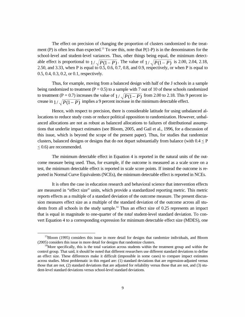
The effect on precision of changing the proportion of clusters randomized to the treat-ment (P) is often less than expected.13 To see this, note that P(1-P) is in the denominators for the school-level and student-level variances. Thus, other things being equal, the minimum detect-able effect is proportional to )1(/1 PP − . The value of )1(/1 PP − is 2.00, 2.04, 2.18, 2.50, and 3.33, when P is equal to 0.5, 0.6, 0.7, 0.8, and 0.9, respectively, or when P is equal to 0.5, 0.4, 0.3, 0.2, or 0.1, respectively.
Thus, for example, moving from a balanced design with half of the J schools in a sample being randomized to treatment (P = 0.5) to a sample with 7 out of 10 of these schools randomized to treatment (P = 0.7) increases the value of )1(/1 PP − from 2.00 to 2.18. This 9 percent in-crease in )1(/1 PP − implies a 9 percent increase in the minimum detectable effect.
Hence, with respect to precision, there is considerable latitude for using unbalanced al-locations to reduce study costs or reduce political opposition to randomization. However, unbal-anced allocations are not as robust as balanced allocations to failures of distributional assump-tions that underlie impact estimates (see Bloom, 2005, and Gail et al., 1996, for a discussion of this issue, which is beyond the scope of the present paper). Thus, for studies that randomize clusters, balanced designs or designs that do not depart substantially from balance (with 0.4 < P < 0.6) are recommended.
The minimum detectable effect in Equation 4 is reported in the natural units of the out-come measure being used. Thus, for example, if the outcome is measured as a scale score on a test, the minimum detectable effect is reported in scale score points. If instead the outcome is re-ported in Normal Curve Equivalents (NCEs), the minimum detectable effect is reported in NCEs.
It is often the case in education research and behavioral science that intervention effects are measured in “effect size” units, which provide a standardized reporting metric. This metric reports effects as a multiple of a standard deviation of the outcome measure. The present discus-sion measures effect size as a multiple of the standard deviation of the outcome across all stu-dents from all schools in the study sample.14 Thus an effect size of 0.25 represents an impact that is equal in magnitude to one-quarter of the total student-level standard deviation. To con-vert Equation 4 to a corresponding expression for minimum detectable effect size (MDES), one
13Bloom (1995) considers this issue in more detail for designs that randomize individuals, and Bloom
(2005) considers this issue in more detail for designs that randomize clusters. 14More specifically, this is the total variation across students within the treatment group and within the
control group. That said, it should be noted that different researchers use different standard deviations to define an effect size. These differences make it difficult (impossible in some cases) to compare impact estimates across studies. Most problematic in this regard are: (1) standard deviations that are regression-adjusted versus those that are not, (2) standard deviations that are adjusted for reliability versus those that are not, and (3) stu-dent-level standard deviations versus school-level standard deviations.

10
would divide it by the total standard deviation of the outcome measure across all students or στ 22 + , yielding
στστ 22
22
2 /)1()1(
+−
+−
= −
nJPPJPPMMDES J
(5)
To translate this expression into one that is more useful for the present discussion re-quires defining an additional parameter, the intra-class correlation or ρ, where
στ
τρ22
2
+= (6)
The intra-class correlation equals the proportion of the total variance across all students (τ2 +σ2) that is due to the variance between schools, τ2. This parameter represents how students are grouped within schools.
At one extreme (perfectly heterogeneous clusters), if the mean values of the outcome were the same for all clusters, τ2 would equal zero, and the intra-class correlation would be zero. Hence, all of the variation across individuals would be within clusters, and none would be be-tween clusters. Consequently, randomizing clusters would be equivalent to randomizing indi-viduals, aside from the difference in the number of degrees of freedom available.
At the other extreme (perfectly homogeneous clusters), if the mean values of the out-come were different for different clusters but the values of the outcome were the same for all individuals in a cluster, σ2 would equal zero and the intraclass correlation would equal one. Hence, all of the variation across individuals would be between clusters, and none would be within clusters. If this were the case, the value of the outcome for one individual in a cluster identifies its values for all other individuals in that cluster.
Rearranging terms in Equation 5 and substituting into it the definition of the intra-class correlation yields
nJPPJPP
MMDES J)1(
1)1(
2−−
+−
= −ρρ (7)
Equation 7 illustrates how the intra-class correlation provides a convenient way to represent τ2 and σ2 in the determination of minimum detectable effect sizes. As can be seen, ρ replaces
)/( 222 σττ + and (1-ρ) replaces )/( 222 στσ + . Thus, ρ represents the between-cluster variance, and (1-ρ) represents the within-cluster variance.

11
Note that in Equation 7 ρ is divided by J, whereas (1-ρ) is divided by J times n. Thus, increasing the number of clusters reduces the influence of both variances on the minimum de-tectable effect, whereas increasing cluster size only reduces the influence of the within-cluster variance. Consequently, doubling the number of clusters randomized will reduce the minimum detectable effect size by far more than will doubling the number of individuals per cluster.
Determining Precision When Baseline Covariates Are Used Now consider how the minimum detectable effect size changes when a covariate or set
of covariates is used to reduce the variance of the school-level random error (τ2), the variance of the student-level random error (σ2), or both.15
nJPPR
JPPRMMDES IC
KJ)1(
)1)(1()1(
)1( 22
−−−
+−−
≈ −ρρ (8)
where:
R2C = the proportion of the random variance between schools that is reduced by
the covariate or covariates (their school-level explanatory power),
R2I = the proportion of the random variance within schools that is reduced by the
covariate or covariates (their individual-level explanatory power),
K = the number of cluster-level covariates used.
First note that the number of degrees of freedom for the minimum detectable effect multiplier changes to MJ-K. This accounts for the loss of one degree of freedom per school-level covariate used. If one school-level covariate were used, the number of degrees of freedom would be J-3; if two school-level covariates were used, the number of degrees of freedom would be J-4; and so on. Student-level covariates do not affect the number of degrees of free-dom and thus do not affect the degrees of freedom multiplier.
15Raudenbush (1997) presents exact expressions that can be used to determine minimum detectable effects
when using a single cluster-level covariate or a single individual-level covariate. These expressions include additional terms not presented here, which do not affect precision appreciably when more than about 20 clus-ters are randomized. We are not aware of corresponding exact expressions for designs that use multiple cluster-level or individual-level covariates. Thus, we present Equation 8 and the findings that follow from it as simple extensions of findings for a single covariate. We believe that these extensions are reasonable approximations for planning research designs because using multiple covariates in a model is similar in spirit (but not exactly the same) as using a composite indicator of these covariates as a single covariate.

12
Other things equal, reducing the number of degrees of freedom increases the minimum detectable effect multiplier. This issue is most important for samples with very few randomized clusters (less than 10), where losing several degrees of freedom can make a big difference.16
The more important differences between Equation 8 for impact analyses with covariates and Equation 7 for impact analyses without covariates are the two new terms in Equation 8, R2
C and R2
I. These terms represent the proportion of the school-level random variance (τ2) and stu-dent-level random variance (σ2) that is reduced or “explained” by the covariate or covariates.17 Specifically:
τττ
2
2*
22 −
=RC (9)
and
σσσ
2
2*
22 −=RI
(10)
where:
τ2* = the school-level variance that remains unexplained by the covariates,
σ2* = the student-level variance that remains unexplained by the covariates.
Thus (1-R2C) and (1-R2
I) represent the proportions of the two random variances that remain when a covariate is added to the analysis. The greater the explanatory power of the covariates is, the more they reduce the unexplained variances; consequently the more they reduce the mini-mum detectable effect size.
School-level covariates can only reduce random variation between schools because their values are constant for all students in a school. Thus, R2
I is zero for designs with school-level covariates only. Student-level covariates can reduce random variation between schools and across students within schools because their individual values can vary across students within schools and their mean values can vary between schools. Nonetheless, as will be shown
16This is not to suggest that multiple school-level covariates can be used with abandon; quite to the con-
trary. Since precision is at such a high premium with cluster randomized designs, even small losses can be im-portant. Therefore one should only use school-level covariates that substantially reduce the school-level vari-ance.
17When using a student-level covariate (as in Equation 4) it is theoretically possible for τ*2 to be larger
than τ2, which would imply a negative value for R2C. This could occur if the correlations between the covariate
and outcome at the student level and school level were in opposite directions. However, this is extremely unlikely to occur for a pretest and post-test that measure the same construct.

13
later, some school-level covariates can reduce minimum detectable effect sizes by as much as or more than student-level covariates.
One common mistake that is made when thinking about the affects of covariates on precision is to focus only on how the intra-class correlation changes from its unconditional value for a design without covariates to a conditional value for a design with covariates. Doing so can be misleading, however, because the intra-class correlation only represents the magni-tudes of the two variances components, τ2 and σ2, relative to each other, whereas precision de-pends on the actual values of their magnitudes. A simple way to see the fallacy that can result from such thinking is to consider the case of a single student-level covariate that substantially reduces τ2 and σ2 and thereby unambiguously improves precision. In principle, it is possible for this covariate to reduce τ2 by proportionately more than it reduces σ2. If so, then the covariate will increase the intra-class correlation. Consequently it is possible for the covariate to simulta-neously increase the intra-class correlation and improve precision.
Equation 8 illustrates how the three design parameters that must be chosen for a study (J, n, and P) and the three empirical parameters that must be taken as given (ρ, R2
C, and R2I)
determine the minimum detectable effect size. Much has been written about the influence of the three design parameters. Much less has been written about the influence of the three empirical parameters.
To understand what is at stake here, consider the minimum detectable effect sizes in Table 1. These illustrative findings were obtained from Equation 8 for a range of values of ρ, R2
C, and R2I, given a sample of 40 clusters with 60 individuals each and half of the clusters ran-
domized to treatment (J = 40, n = 60, and P = 0.5). Each panel in the table represents a different value for the intra-class correlation (ρ). (Note that this is the “unconditional” intra-class correla-tion without any covariates.)
The minimum detectable effect size in the upper left-hand corner of each panel repre-sents a cluster-randomized design without covariates and thus values of zero for R2
C and R2I.
For example, when ρ equals 0.15, the minimum detectable effect size for a design with no co-variates is 0.37. Now consider what happens when a school-level covariate is added to the analysis. First recall that such covariates can increase R2
C but cannot affect R2I. In the table this
is equivalent to moving from left to right in a row. When doing so, the minimum detectable ef-fect size declines rapidly. Thus, increasing R2
C produces dramatic improvements in precision, all else being equal. For example, when R2
C reaches 0.8 (given ρ = 0.15 and R2I = 0.0), the
minimum detectable effect size falls to 0.19, which is roughly half of its original value. This

14
improvement in precision is equivalent to that which would be produced by a fourfold increase in the number of clusters (schools) randomized.18
Now consider what happens when a student-level covariate is added to the analysis. Recall that such covariates can increase both R2
I and R2C. In the table, increasing R2
I is equiva-lent to moving down a column in a panel. This makes very little difference to the minimum de-tectable effect size.19 For example, moving down the first column in the middle panel indicates that when R2
I equals 0.8 (given ρ = 0.15 and R2C = 0.0), the minimum detectable effect size
equals 0.36. This is almost identical to the corresponding minimum detectable effect size with-out covariates. Thus, reducing the student-level variance has almost no effect on precision. This finding is consistent with the fact that increasing the number of individuals per cluster often has little effect on precision (Bloom, 2005). Nonetheless, an individual-level covariate can also re-duce the cluster-level variance, thereby increasing R2
C, which can reduce the minimum detect-able effect appreciably.
Lastly, consider how the unconditional intra-class correlation (ρ) affects precision by comparing the minimum detectable effect sizes of corresponding cells in the three panels in Ta-ble 1. As can be seen, other things being equal, a higher intra-class correlation creates a larger minimum detectable effect size and thus produces less precision. For example, a design with no covariates (R2
C = R2I = 0) has a minimum detectable effect size of 0.30, 0.37, or 0.42 when ρ
equals 0.10, 0.15, or 0.20, respectively.
Table 1 illustrates the profound effect that the three empirical parameters can have on the precision of impact estimates from a cluster-randomized study. Thus, to design such studies, it is crucial to have some knowledge of the likely values of these parameters. The remainder of this paper presents such information for situations where the outcome of interest is student achieve-ment and the clusters to be randomized are schools. This information is based on extensive stu-dent-level data from the administrative records of five urban school districts. Findings are pre-sented first for elementary schools (grades 3 and 5), then for middle schools (grade 8) and high schools (grade 10). These findings are presented for outcome measures based on the results of standardized tests in reading and in math. Data from all five districts are available for elementary schools, whereas data from only two districts are available for middle schools and high schools. All results are based on estimates of ρ, R2
C, and R2I, which are presented in the appendix.
18This point can be seen from Equation 8, which illustrates that the minimum detectable effect size is ap-
proximately proportional to the square root of the number of clusters randomized (J). Thus, other things being equal, one must increase the number of clusters randomized by a factor of four to reduce the minimum detect-able effect size by a factor of two.
19Centering the values of an individual covariate on its mean for each cluster would increase R2I but not
R2C. Thus, for cluster-randomized studies this is not a good practice.

15
Research Design Questions Addressed Before presenting the findings of the present analysis it is useful to clarify the research
design questions they address. Table 2 presents two categories of such questions. The first cate-gory contains a series of core questions, which involve the most basic issues that arise in the use of covariates for increasing precision in studies that randomize schools to measure the effects of educational interventions. The second category contains a series of further questions that have arisen from our experiences and the experiences of our colleagues in planning such studies.
Core Questions
The first and most fundamental question to address is: By how much can precision be improved through the use of data on pretests? If precision can be improved by a lot, then many fewer schools can be randomized for given studies, their costs will be reduced accordingly, and more studies can be supported by existing funding sources.
A related sub-question that also has important financial implications is: How much preci-sion can be gained through the use of school-level pretests versus student-level pretests? Data on school-level pretests (mean scores for schools during baseline years) often can be obtained quickly and cheaply from electronic reports that are publicly available on state or local Web sites. Data on student-level pretests (individual scores during baseline years) must be obtained from the adminis-trative records of local or state educational agencies, which requires considerably more effort and expense. Thus, substantial cost savings can be had if school-level pretests can be used.
There are several reasons to expect school-level covariates to perform as well as student-level covariates. First, correlations across aggregate entities (especially, large aggregate entities) tend to be much higher than those across individuals.20 For example, several decades ago, when most social science research was based on aggregate data for census tracts, communities, states, countries, etc., prevailing expectations for correlations were quite high — often in excess of 0.9. But recently, as modern technology has facilitated the analysis of large micro-datasets on indi-viduals, expectations for correlations have become much lower. This suggests that R2
C typically will be substantially higher than R2
I unless the number of students per school is very small. Sec-ond, since the school-level variance (τ2) is usually the binding constraint on precision, increasing R2
C is usually far more important than increasing R2I in order to improve precision.
The next core question acknowledges the reality that because most educational inter-ventions are complicated and take considerable time to implement, their evaluations often must
20This is partly because the reliability of an aggregate-level measure is greater than that of an individual-
level measure; thus, correlations are greater for aggregate measures.

16
span several follow-up years. Thus, in designing such evaluations it is important to ensure ade-quate precision not only for their first year of follow-up but for subsequent years as well. This raises the issue of how the predictive power of a baseline covariate declines as the gap in time between it and follow-up measures increases. The more quickly this predictive power declines, the larger the study sample must be to ensure adequate precision for later follow-up years.
The next three questions consider how precision varies across subjects (reading and math), education levels (elementary school, middle school, and high school), and local school districts (the five districts in the present analysis). Findings for reading and math are important because of the need to design evaluations of interventions for both subjects. Findings for differ-ent education levels are important because of the need to evaluate interventions targeted on these levels. However, almost all of what is known currently about the precision of studies that randomize schools to evaluate educational interventions is for elementary schools.
Findings for different school districts are important in order to assess how applicable they are likely to be for planning future studies. To the extent that findings vary little across dis-tricts, researchers can be more confident in using these findings to plan future studies. To the extent that findings vary widely across districts, it becomes more important for researchers to estimate planning parameters directly from baseline data for the districts in which their studies will be conducted (which often is not possible).
The last of the core questions considers how the parameters that determine precision vary across years in the same school district. This question relates to the amount of risk that re-searchers are taking (and thus how conservative they should be) when making assumptions about future values of these parameters in order to plan a study. To the extent that these parame-ters are stable over time in a given district, it is safe to plan a study on their estimates from past data. To the extent that these parameters vary over time, researchers must be conservative about their likely future values.
Further Questions
The next series of questions in Table 2 represents alternative specifications of covariates to improve precision. Some of these questions are about potential ways to improve precision by more than is possible using a single pretest. Others of these questions are about potential fall-back positions or second-best solutions to consider when it is not possible to obtain appropriate pretest data.
The first question in this category considers the possible improvement in precision that can be achieved by using pretests for two baseline years instead of one. For school-level pretests this would require data on mean test scores for each of two baseline years. For student-level pre-tests this would require data on individual student tests scores for each of two baseline years. It

17
stands to reason that pretests for two baseline years should have greater predictive power (higher R2
C or R2I) and thus produce greater precision than a pretest for one baseline year. But it is an em-
pirical question as to just how much difference a pretest for a second baseline year makes.
The next question considers using a school-level pretest and a student-level pretest to-gether. Once again, it stands to reason that two pretests should improve precision by more than one. But it is an empirical question as to how much difference the second pretest makes.
The third question considers how much precision can be achieved if pretest data are not available and only demographic characteristics can be used as covariates. This is not likely to occur for evaluation studies based on data from local school districts, but it might occur for studies based on data from national surveys. The fourth question takes a different tack with re-spect to using demographic data. It considers the extent to which adding demographic covari-ates to a pretest can improve precision.
The fifth question considers situations where the pretest used to measure baseline out-comes differs from the post-test used to measure follow-up outcomes. Such situations reflect the real-world tendency for states and districts to frequently change the tests they use to assess the progress of students and schools. One might expect less predictive power, and thus less preci-sion, in situations where baseline outcomes and follow-up outcomes are measured using differ-ent tests than when they are measured using the same test. But, for school-level pretests, much of the basis for their predictive power might be differences among schools (“school effects”) that are fairly stable over time and tests. Thus, it might be possible to achieve values for R2
C that are almost as high when post-tests and pretests differ as when they are the same.
The last two questions in the table consider what precision is likely to be if a study fo-cused on either of two sub-groups of schools within a district: those with especially high con-centrations of low-income students and those with especially low past student performance. There are at least two reasons to focus on these sub-samples. First, they are the most frequent subject of evaluations of educational interventions funded by the U.S. Department of Education and private foundations. Thus, focusing on precision for these types of schools is relevant to the design of many studies. Second, focusing on these sub-samples represents a simplified version of a related approach to improving precision — that of stratifying clusters into blocks. This ap-proach is intended to create blocks of schools that are as similar as possible before randomiza-tion. By randomizing within blocks one can ensure that the subsequent treatment and control groups are more similar to each other than they would have been without blocking. This in turn can reduce the standard errors of impact estimates (although often at the cost of reducing de-

18
grees of freedom).21 However, if one is already adjusting for a baseline covariate through a sta-tistical model, it is not clear how much more precision can be gained by blocking.
In the present context this situation could occur as follows. If one switched from a sam-ple of all schools in a district to a sub-sample of those that were either especially low-income or especially low-performing or both, the variation in future outcomes for the sub-sample most likely would be smaller than that for the full sample (perhaps by a lot). This means that the un-conditional intra-class correlation for the sub-sample would be less than that for the full sample. So, in this regard, precision for the sub-sample would be enhanced relative to that for the full sample. However, given the restricted variation in outcomes for the sub-sample, the additional explanatory power of covariates is likely to be lower for the sub-sample than for the full sample. If so, then it is not clear whether the sub-sample will have more precision, less precision, or about the same precision as the full sample for a given research design and sample size.
The preceding questions reflect a series of hypotheses about the abilities to improve preci-sion of different types of covariates, different combinations of covariates, and/or different sub-samples of schools. The following sections provide empirical evidence to test these hypotheses.
Overview of the Empirical Analysis The present empirical analysis is based on individual data for thousands of students
from hundreds of schools located in five urban school districts. Elementary school analyses fo-cus on reading and math test scores in grades three and five using data from all five districts.22 Middle school analyses focus on reading and math test scores in grade eight and the high school analyses focus on reading and math test scores in grade 10. Data for middle school and high school analyses were only available for two of the five districts. All analyses were also repli-cated for as many years as possible in each district.
Table 3 briefly describes the districts, schools, and students in the sample for the present analysis. First note that the districts in the sample are fairly large. They represent from 25 to 168 elementary schools, 17 to 41 middle schools, and 11to 32 high schools. The average elementary school in each district had 57 to 75 third-grade students who were tested in a given year; the average middle school had 196 to 297 eighth-grade students; and the average high school had 234 to 269 tenth-grade students. In two districts, students were predominantly black; in two other districts they were a mix of blacks and Hispanics; and in the fifth district information was not available on their background characteristics. In the three districts where data on economic
21The use of blocking to improve the precision of cluster-randomized studies is discussed by Raudenbush,
Martinez, and Spybrook (2005), Bloom (2005), Donner and Klar (2000), and Murray (1998). 22Available data made it necessary to use grade six instead of grade five for one district.

19
status were available for elementary schools, the percentage of students who were categorized as low-income ranged from 41 percent to 79 percent.
The first step in the present analysis for a given grade, subject, district, and year was to estimate the unconditional values of τ2 and σ2 (without covariates) and use these estimates to compute the unconditional intra-class correlation, ρ. This factor reflects how students in a given grade were clustered within schools in the district that year. The second step in the analysis was to estimate the conditional values of τ2
* and σ2* for different baseline covariate specifications.
For each specification the relationships between the conditional and unconditional values of the two variances were used to compute R2
C and R2I. The mean values of these parameter estimates
(across years for a given grade, subject, and district) are presented in a series of tables to provide an empirical guide for planning future evaluation studies. In addition, the mean estimated values of the three empirical parameters (ρ, R2
C, and R2I) were used to compute minimum detectable
effect sizes for alternative sample designs for each grade and subject.
Because of the very large number of findings produced it was necessary to develop a strategy for presenting them in a manner that provides both an effective way to address the re-search design questions posed above and adequate detail for helping researchers plan future studies. The remainder of the paper is thus structured as follows.
Part II of the paper presents findings for elementary schools. It begins with a detailed presentation of findings for third grade reading. The remainder of this part focuses on a consoli-dated summary of findings for third grade and fifth grade reading and math. This avoids the re-dundancy that would occur if all detailed findings were presented and facilitates comparisons of findings across grades and subjects. Corresponding detailed findings are presented in the ap-pendix. Part III of the paper presents summarized findings for middle schools and high schools, whose detailed findings are presented in the appendix to this paper. Part IV of the paper reflects briefly on the implications of these findings.

20
Part II: Findings for Elementary Schools
This part of the paper presents findings for elementary schools.
Detailed Findings for Third Grade Reading The discussion of findings begins with a complete examination of the detailed findings
for third grade reading. This serves several purposes. First it introduces readers to the material in enough detail so that they can understand the full range of findings presented in the text and ap-pendix. Second it provides a template for presenting the findings for other grades and subjects. Third it identifies most of the key issues, findings, and implications that apply to the other grades and subjects.
Precision with a Single Pretest
Tables 4 through 8 present detailed findings for third grade reading. Table 4 addresses the first two core research design questions. It presents estimates of minimum detectable effect sizes for a research design with no covariates or a single pretest, given the mean estimated val-ues (across years) of ρ, R2
C, and R2I for these covariate specifications in each district. Minimum
detectable effect sizes are based on the assumptions of 80 percent statistical power and 0.05 sta-tistical significance for a two-tail hypothesis test with 60 third graders per school. Results in the top, middle, and bottom panels are for samples of 20, 40, and 60 schools, respectively, with half of the schools in each case randomized to treatment
The first five columns in the table present findings by district. The last column presents the mean values of the corresponding district results (with each district weighted equally). Means that are not based on data for all districts are presented in parentheses. Although these findings for subsets of districts are important in their own right, they are not fully comparable to findings for all districts.
Each row in a panel presents findings for a particular covariate specification. The first row presents findings for a design without covariates, which is the starting point for each analy-sis. The next three rows present findings for school-level pretests that are lagged one, two, and three years (Y-1, Y-2, and Y-3). These findings for school-level pretests are used to predict the precision that might be expected during the first, second, and third follow-up years of a study, respectively. The final three rows in each panel present corresponding results for student-level pretests (y-1, y-2, and y-3).

21
Before interpreting these results it is necessary to address the question: How much pre-cision is needed for an educational evaluation?23 In other words, how small must its minimum detectable effect size be? Stated yet another way, must the study be able to detect large effects, moderate effects, or small effects according to prevailing standards (discussed below)? From an economic perspective, the answer to this question is that the design should be able to detect the smallest effect that would enable an intervention to break even in a cost-effectiveness analysis. From a political perspective, the answer is that the design should be able to detect the smallest effect that would be deemed important by the public or by public officials. From a program-matic perspective, the answer is that the study should be able to detect an effect that, judging from the performance of similar programs, is likely to be attainable.
There is no universal standard for making such judgments. One widely used approach is that of Cohen (1977), who proposed that minimum detectable effect sizes of roughly 0.20, 0.50, and 0.80 be considered small, medium, and large, respectively. Lipsey (1990) provided empiri-cal support for this characterization by examining the actual distribution of 102 mean effect size estimates reported in 186 meta-analyses that together represent 6,700 studies with 800,000 sample members. Consistent with Cohen’s categorization, the bottom third of this distribution ranged from 0.00 to 0.32, the middle third ranged from 0.33 to 0.55, and the top third ranged from 0.56 to 1.20.
However, recent research suggests that, at least for education interventions (and perhaps for other types of interventions as well), much smaller effect sizes should be considered sub-stantively important, and thus greater precision might be needed than is suggested by Cohen’s categories. Foremost among the findings motivating these new expectations are those from the Tennessee Class Size Experiment. These findings indicate that reducing elementary school classes from a standard size of 22 to 26 students to a reduced size of 13 to 17 students increases average student performance by an effect size of roughly 0.1 to 0.2 (Nye, Hedges, and Konstan-topoulos, 1999). This landmark study of a major education intervention suggests that even big changes in schools produce what by previous standards would have been considered small ef-fects on student achievement.
Another important piece of related research is that by Kane (2004), who found that, on average nationwide, a full year of elementary school attendance increases students’ reading and math achievement by an effect size of only 0.25. Thus, an education intervention that has a positive effect size only half as large as this (0.125) would seem to qualify as a noteworthy suc-cess. Further reinforcing these findings are results published by the National Center for Educa-tion Statistics (1977) indicating that, on average nationwide, high school students increase their reading achievement by an effect size of 0.17 annually and math achievement by 0.26 annually.
23The following four paragraphs are a revised excerpt from Bloom (2005), pp. 131-32.

22
This gain represents the effect of attending school plus the effect of all other factors that are in-fluencing student development throughout the year. Thus, again the message is clear: program effect sizes for student achievement of as little as 0.10 to 0.20 might be policy-relevant.
At the present time, standards for interpreting the magnitudes of educational impacts and thus determining the requisite precision of educational evaluations are in a state of flux. However, because numerous recent evaluations have been designed to detect effect sizes of roughly 0.20, the present paper uses this value as a benchmark or standard of comparison.24
Now consider the findings in Table 4, beginning with those for a design without covari-ates. The mean value of the minimum detectable effect size for this most basic design is 0.57 for 20 randomized schools (ranging from 0.47 to 0.63 across districts), 0.39 for 40 randomized schools (ranging from 0.33 to 0.44 across districts), and 0.32 for 60 randomized schools (rang-ing from 0.27 to 0.35 across districts). Hence, the design does not appear to be capable of achieving the prevailing standard benchmark for precision without randomizing many more than 60 schools (about 150), which most likely would be prohibitively expensive.
The next three rows in each panel of Table 4 illustrate how an aggregate pretest lagged one, two, or three years (Y-1, Y-2, and Y-3) can vastly improve this situation for the first, second, or third follow-up years of an evaluation study. During the first follow-up year, when the time lag between the post-test and pretest is one year, the mean minimum detectable effect size for all dis-tricts is 0.37, 0.26, and 0.21 for 20, 40, and 60 randomized schools respectively.25 Thus, according to these estimates, randomizing 60 schools when using such a covariate would achieve the pre-vailing benchmark for precision, and randomizing 40 schools would approach doing so. (Note that to obtain these samples might require operating a study in multiple districts.)
During the second follow-up year of an evaluation study, when the time lag between the post-test and pretest is two years, the mean minimum detectable effect size for all districts is slightly larger: 0.40, 0.28, and 0.23 for 20, 40, and 60 randomized schools, respectively. This represents the slightly lower predictive power of a pretest for a two-year time period. During the third follow-up year, the mean minimum detectable effect size is slightly larger yet, although it is not directly comparable to the others because it represents only three of the five school dis-tricts in the analysis.
24Two authors of the present paper (Bloom and Rebeck Black) are working with Mark Lipsey of Vander-
bilt University and Carolyn Hill of Georgetown University on a project funded by the U.S. Department of Edu-cation to examine “The Uses and Abuses of Effect Size Measures.” The goal of this project is to develop em-pirical benchmarks for assessing effect sizes from educational interventions.
25The improvement in precision produced by a school-level pretest for the first follow-up year is equiva-lent to more than doubling the number of schools randomized.

23
Overall, the mean findings suggest that, by randomizing 40 to 60 schools, one can ap-proach or attain the prevailing standard for precision during the first three years of an evaluation study. However, there is considerable variation in the findings across districts, and hence there remains an important element of uncertainty about the likely precision of a study based on schools in a particular district or group of districts. We illustrate one approach to quantifying this uncertainty in the final section of the paper.
Now consider whether student-level pretests, which are more difficult and costly to ob-tain, can improve precision by appreciably more than school-level pretests. Findings in the table suggest that the answer to this question is no. This can be seen by comparing the minimum de-tectable effect size during the first follow-up year (the only time for which data from all districts are available) for a student-level pretest (y-1) and a school-level pretest (Y-1). For example, with 40 randomized schools, the mean minimum detectable effect size during the first follow-up year is 0.26 for both a school-level and a student-level pretest. And in no district does the student-level covariate appreciably outperform the school-level covariate. This implies that school mean reading scores for last year’s third graders provide as much precision as second grade scores for each of this year’s third graders.
Precision with Other Covariate Specifications and School Samples
Table 5 addresses most of the remaining research design questions posed earlier. It pre-sents estimated minimum detectable effect sizes for alternative covariate specifications and school samples given a balanced allocation of 40 randomized elementary schools with 60 stu-dents per school.26 District E is not included in this table because corresponding findings for the district are not available.27
The first panel in the table presents results for alternative covariate specifications based on data for the full sample of schools from each district. The second panel presents re-sults for the simplest pretest specifications based on data for a sub-sample of schools whose concentration of poverty (measured by their percentage of students eligible for free lunches) was above their district average. The third panel presents results for the simplest pretest speci-fications based on data for a sub-sample of schools whose past student performance was be-low their district average.
26Table 5 only reports findings for 40 randomized schools (the middle sample size in Table 4) in order to
reduce the number of finding to a manageable number. 27Findings for District E were obtained from Bloom, Bos, and Lee (1999). Because the data for this analy-
sis are no longer available, it was not possible to present findings for covariate specifications or sub-samples of schools that were not in the original analysis.

24
The first five rows in the table address the question: How much more precision can be obtained by adding a second pretest? The answer to this question for school-level pretests only (Y-1 and Y-2) is that adding a pretest for a second baseline year produces virtually no improve-ment. The average minimum detectable effect size is approximately 0.27 for one or both pre-tests.28 The same answer applies to student-level pretests only (y-1 and y-2), although to make this assessment requires focusing directly on the findings for Districts A and C (which are the only districts for which two consecutive student-level pretests are available). As can be seen, there is almost no difference between the precision for one individual-level pretest and that for two in either district.
A somewhat more encouraging result occurs with the addition of a school-level pretest to a student-level pretest or vice versa (Y-1 and y-1). This is perhaps because the two sources of information being combined differ more from each other than is the case for two pretests of the same kind. Adding a student-level pretest to a school-level pretest reduces the mean minimum detectable effect size from 0.27 to 0.25. Adding a school-level pretest to a student-level pretest reduces the mean minimum detectable effect size from 0.28 to 0.25. Findings for all but one district are consistent with this pattern.
The next two rows in the table present estimates of minimum detectable effect sizes when school-level or student-level math scores (Z-1 or z-1) are used as a pretest for a third grade reading post-test. These findings provide conservative estimates of the precision that one might expect when a pretest and post-test represent different tests in the same subject. This situation can arise when school districts change their student assessments, which they do frequently. Re-sults in the table indicate that even if a pretest is in the “wrong” subject, it can improve precision dramatically. A school-level math pretest reduces the mean minimum detectable effect size for a reading post-test from 0.41 without covariates to 0.29. This is equivalent to doubling the num-ber of schools randomized. Similarly, a student-level math pretest reduces the mean minimum detectable effect size to 0.31. In both cases, the resulting precision is almost but not quite as good as that for a pretest and post-test in the same subject. Thus, just because a school district changed its student assessment, does not necessarily mean that the baseline data available for use as pretests cannot improve precision substantially.
The last three rows in Table 5 for the sample of all elementary schools from each dis-trict present estimates of minimum detectable effect sizes that would result if student demo-graphic characteristics, X, were used as covariates either alone or in conjunction with a school-
28The table indicates that the minimum detectable effect size is slightly smaller for two school-level pre-
tests than for one, at three of the four districts and identical at the fourth. However, the mean minimum detect-able effect sizes across districts are the same for one and two pretests. This apparent inconsistency is due to rounding.
25
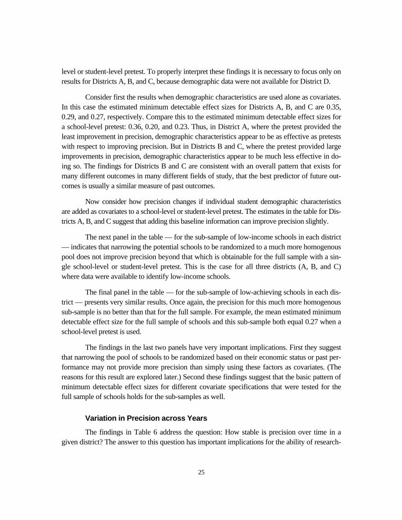
level or student-level pretest. To properly interpret these findings it is necessary to focus only on results for Districts A, B, and C, because demographic data were not available for District D.
Consider first the results when demographic characteristics are used alone as covariates. In this case the estimated minimum detectable effect sizes for Districts A, B, and C are 0.35, 0.29, and 0.27, respectively. Compare this to the estimated minimum detectable effect sizes for a school-level pretest: 0.36, 0.20, and 0.23. Thus, in District A, where the pretest provided the least improvement in precision, demographic characteristics appear to be as effective as pretests with respect to improving precision. But in Districts B and C, where the pretest provided large improvements in precision, demographic characteristics appear to be much less effective in do-ing so. The findings for Districts B and C are consistent with an overall pattern that exists for many different outcomes in many different fields of study, that the best predictor of future out-comes is usually a similar measure of past outcomes.
Now consider how precision changes if individual student demographic characteristics are added as covariates to a school-level or student-level pretest. The estimates in the table for Dis-tricts A, B, and C suggest that adding this baseline information can improve precision slightly.
The next panel in the table — for the sub-sample of low-income schools in each district — indicates that narrowing the potential schools to be randomized to a much more homogenous pool does not improve precision beyond that which is obtainable for the full sample with a sin-gle school-level or student-level pretest. This is the case for all three districts (A, B, and C) where data were available to identify low-income schools.
The final panel in the table — for the sub-sample of low-achieving schools in each dis-trict — presents very similar results. Once again, the precision for this much more homogenous sub-sample is no better than that for the full sample. For example, the mean estimated minimum detectable effect size for the full sample of schools and this sub-sample both equal 0.27 when a school-level pretest is used.
The findings in the last two panels have very important implications. First they suggest that narrowing the pool of schools to be randomized based on their economic status or past per-formance may not provide more precision than simply using these factors as covariates. (The reasons for this result are explored later.) Second these findings suggest that the basic pattern of minimum detectable effect sizes for different covariate specifications that were tested for the full sample of schools holds for the sub-samples as well.
Variation in Precision across Years
The findings in Table 6 address the question: How stable is precision over time in a given district? The answer to this question has important implications for the ability of research-

26
ers to predict precision and thereby plan future studies. If precision varies markedly from year to year in a district, it is necessary to make conservative assumptions about likely future precision. If precision is stable, less conservative assumptions are viable.
The table presents the range (from lowest to highest) of minimum detectable effect sizes that are implied by the estimated parameters for each district in the present analysis during each year for which appropriate data were available. Because data for the two most basic co-variate specifications were available for more than one year in every district, findings for these specifications are presented. As can be seen, sometimes there is considerable variability from year to year in the likely minimum detectable effect size for a given district, and sometimes there is little variation. This is the case for the full sample of schools from each district, its sub-sample of low-income schools, and its sub-sample of low-performing schools. Unfortunately, there is no known way to predict where and when precision might be variable or stable. There-fore, when planning a study, one probably should be relatively conservative.
Parameters Estimates
Table 7 provides further detail about the preceding findings by presenting the mean es-timated values of the three empirical parameters upon which they are based. These results are presented for all covariate specifications that were examined for the full sample of schools. The first row in the table lists the mean value of the unconditional intra-class correlation, ρ (without covariates), for each district. Subsequent rows present the mean estimated values of R2
C (the proportion of the school-level variance that is predicted by a covariate) and R2
I (the proportion of the student-level variance that is predicted by a covariate).
The mean value of ρ varies across districts from a low of 0.15 to a high of 0.22. As dis-cussed in Part IV, this is consistent with most past research.
The next panel in the table presents values of R2C and R2
I when school-level pretests are the only covariates used. First note that R2
I is zero for all of these covariate specifications. This is because the value of a school-level covariate is the same for all students from a given school and thus cannot covary with their test scores. Next, note that R2
C varies in predictable ways across the different types and combinations of pretests. It declines as the gap in time increases between post-tests and pretests, and it is larger for combinations of pretests than for single pre-tests. Lastly, note that for any given covariate specification, R2
C varies substantially across dis-tricts. For example, it ranged from a low of 0.31 in District A to a high of 0.77 in District B for a single school-level pretest lagged one year (Y-1).
The middle panel in the table presents values of R2C and R2
I when student-level pretests are the only covariates used. Because these pretests can vary across and within schools, their values for R2
C and R2I are non-zero. These values also vary in predictable ways: declining as the

27
time-lag between pretests and post-tests increases and being higher for combinations of pretests than for single pretests.
It is particularly useful to compare the effects of student-level and school-level pretests on R2
C and R2I because doing so illustrates why student-level pretests do not provide superior
precision. The simplest and clearest way to make this comparison is to focus on pretests lagged one year (y-1 and Y-1) for which data from all districts are available. In terms of R2
C, the school-level pretest has a slight advantage in all but one district, where it had a considerable advantage. In terms of R2
I, the student-level pretest has an advantage that ranges from small to substantial. Recall, however, that R2
C represents the reduction in τ2 produced by a covariate, whereas R2I
represents its reduction in σ2. Because τ2 has a much larger effect on precision than does σ2 for studies that randomize schools to study impacts on student achievement, the higher R2
I for stu-dent-level pretests does not offset its lower R2
C. Hence, precision for the student-level pretest is not greater than that for the school-level pretest.29
The bottom panel in the table presents values of R2C and R2
I for the other major covari-ate specifications included in the present analysis. These findings are presented because they are relevant to researchers who are considering the use of such specifications.
Parameters Ranges Across School Samples and Time
Table 8 presents the last in the series of detailed findings for third grade reading. It illus-trates: (1) the differences in the values of ρ, R2
C, and R2I for all elementary schools from a dis-
trict and those for their sub-samples of low-income and low-performing schools and (2) the variability of these parameter estimates over time. Each cell in the table represents a range of estimates across the several years for which data were available from each district. These find-ings are presented for a school-level pretest (Y-1) and a student-level pretest (y-1).
Differences between the parameter estimates for the full samples of schools and those for the sub-samples explain why precision is no better for the sub-samples than for the full sam-ples, even though the sub-samples are considerably more homogeneous. Because of this greater homogeneity, ρ is typically much smaller for the sub-samples. This can be seen by comparing the ranges of estimates of ρ for the three groups of schools in each district. However, it is also the case that R2
C is typically much lower for the sub-samples of schools than for the full sam-ples. This is because the restricted variation in the outcome measure across schools in the sub-samples provides less of a margin for school-level covariation with a pretest. Another way to explain this phenomenon is that the restricted variation in outcomes for schools in the sub-
29For a given student-level pretest specification R2
C is usually much larger than R2I. This reflects the gen-
eral tendency for correlations among aggregates to be higher than correlations among individuals.

28
samples contains less “signal to noise” than is the case for the full samples. Because moving to a more homogeneous sub-sample of schools reduces both ρ and R2
C, the overall effect on preci-sion is negligible.
Lastly note that moving to a sub-sample of schools has little or no effect on R2I. This is
because restricting the range of variation in outcomes across schools by choosing a sub-sample of them does not necessarily affect the variation in individual outcomes within schools and thus does not necessarily affect the margin for covariation with individual pretests.30
Summary Findings for Elementary Schools This section compares summary findings for third grade reading with those for third
grade math and fifth grade reading and math. The appendix presents all of the detailed findings for third grade math and fifth grade reading and math (their equivalents to Tables 4 – 8).
Table 9 presents the mean minimum detectable effect size by grade and subject for de-signs that have either no covariates or a single pretest. When comparing these findings across grades and subjects note that outcome data for third grade reading and math were available from all five districts, whereas outcome data for fifth grade reading and math were not available from District D, and outcome data for sixth grade were used to approximate fifth grade for District E. These differences in districts could generate differences in findings. In addition, data were not available for certain covariate specifications in some districts, even when outcome data were available. These cases, whose findings are presented in parentheses, represent even fewer dis-tricts (sometimes only one) and thus may vary even more.
Nevertheless, the findings in Table 9 indicate an extraordinary degree of consistency across grades and subjects. Consider the results for a design with no covariates. The mean esti-mated minimum detectable effect size ranges from 0.38 to 0.40 when 40 schools are random-ized. This implies that the mean estimated unconditional intra-class correlation, ρ, is almost identical for the grades and subjects being compared. Results for school-level pretests are equally consistent. When 40 schools are randomized, the mean minimum detectable effect size for Y-1 is 0.26 in all cases, and its counterpart for Y-2 ranges from 0.28 to 0.29. This implies that the average estimated values of R2
C are highly consistent across grades and subjects. Corre-sponding results for student-level pretests are only slightly less consistent, ranging from 0.26 to 0.30 for y-1 when 40 schools are randomized.
30In theory, it is possible that the amount of student-level variation (and thus co-variation) for the sub-
samples of low-income or low-performing schools could differ from that for the full sample. This was not the case for the present study.

29
Overall, then, the findings strongly suggest that, in the absence of specific data to the contrary for the school district or districts in which a planned study is to be conducted, the best guess is that randomizing 20 schools with a single school-level or student-level pretest will pro-duce a minimum detectable effect size of about 0.38 or 0.39, randomizing 40 schools will pro-duce a minimum detectable effect size of about 0.26 or 0.27, and randomizing 60 schools will produce a minimum detectable effect size of about 0.21 or 0.22. Thus, it appears that randomiz-ing 40 to 60 schools is required in order to approach or reach the current standard of 0.20 for minimum detectable effect sizes.
Table 10 presents the mean estimated minimum detectable effect sizes for the remain-ing covariate specifications and for sub-samples of low-income schools or low-performing schools given 40 randomized schools. Only findings for Districts A – D are available for third grade and only findings for Districts A – C are available for fifth grade. Furthermore, data were not available from all of these districts for some covariate specifications or sub-samples of schools. These findings are reported in parentheses.
Even with their smaller samples of districts the results in Table 10 exhibit a high level of consistency across grades and subjects. In addition, patterns of findings across covariate specifications and sub-samples that were reported earlier for third grade reading hold with strik-ing regularity for the other grades and subjects.
For example, in all cases:
• Using a pretest improves precision dramatically.
• The precision of a school-level pretest is as great as or greater than that for a student-level pretest.
• Adding a school-level pretest for a second baseline year improves precision by very little.
• Replacing a school-level pretest with another in a different subject reduces precision by very little.
• Narrowing the sample of schools to a more homogeneous group with below-average performance does not improve precision if a pretest is used as a co-variate.
The next question to address is: How do corresponding findings for middle schools and high schools compare to those for elementary schools?

30
Part III: Findings for Middle Schools and High Schools
This section examines the likely precision of studies that randomize middle schools or high schools to measure the effects of educational interventions on student achievement. To do so it presents summary estimates of minimum detectable effect sizes for eighth grade and tenth grade reading and math. These estimates are computed in the same way as were those for ele-mentary schools except they assume 250 students in a grade per school (instead of 60 for ele-mentary schools) and they could only be estimated for Districts A and C. Detailed estimates comparable to those in Tables 4 – 8 for third grade reading are presented in the appendix for eighth grade and tenth grade reading and math.
Table 11 presents estimated minimum detectable effect sizes for designs with no co-variates or a single pretest given 20, 40, or 60 randomized schools. In many ways, these find-ings are similar to those for elementary schools. For example: (1) precision without a covariate for secondary schools is comparable to that for elementary schools; (2) a school-level or student level pretest greatly improves precision for both types of schools; (3) a student-level pretest does not improve precision by more than does a school-level pretests for both types of schools; and (4) some precision is lost as the time lag between a pretest and post-test increases for both types of schools.
On the other hand, there is a very important difference between the findings for middle schools and high schools and those for elementary schools. Specifically, pretests reduce minimum detectable effect sizes by proportionately much more for middle schools and high schools. Indeed precision with a pretest improves consistently and substantially from elementary schools to middle schools to high schools. This progression implies a corresponding increase in the values of R2
C. To see this, compare the minimum detectable effects for Y-1 in Table 11 for middle schools and high schools with their counterparts in Table 4 for elementary schools. As can be seen, they are largest for elementary schools, appreciably smaller for middle schools, and appreciably smaller yet for high schools. These differences are not due to the fact that elementary school findings are aver-aged across all five districts whereas those for middle schools and high schools are averaged only across Districts A and C. Detailed findings in the appendix indicate that even within these two districts, where data for all educational levels are available, there is a pronounced reduction in minimum detectable effect sizes as the educational level increases.31
Perhaps the most important feature of these findings is what they imply for the number of middle schools or high schools that must be randomized to attain the prevailing standard of
31Furthermore, having more students per grade in secondary schools than in elementary schools does not
affect their relative precision appreciably.

31
0.20 for minimum detectable effect sizes. Recall that the findings in Table 4 indicate that roughly 60 elementary schools are needed to achieve this standard. But the findings in Table 11 indicate that only about 40 middle schools or 20 high schools would be needed to do so.
Since there are no existing distinctions between standards of precision for studies of secondary schools versus standards for studies of elementary schools, the present findings sug-gest that experimental samples can be much smaller for secondary schools. On the other hand, there is a small but growing body of evidence which suggests that greater precision may be needed for secondary schools than for elementary schools. The reason for this is that develop-mental trajectories for reading and basic math are much flatter in later grades than in early grades. Hence, annual gains in reading or math (in effect size) are much larger for elementary school students than for high school students (Bloom and Lipsey, 2005, and Kane, 2004). Therefore, the ability of interventions to create impacts on these outcomes (their value-added) might be more limited for later grades. To address this issue is well beyond the scope of the pre-sent paper, however.32 Another factor to consider when assessing these findings that is beyond the scope of the present analysis is the extent to which they do or do not apply to other out-comes that are important for secondary schools, such as measures of credits accumulated, rates of on-time transitions from one grade to the next (especially ninth grade to tenth grade), or achievement in more advanced subjects that are only taught at the secondary level.
Table 12 presents estimates of minimum detectable effects size given 40 randomized schools for a broad range of covariate specifications and alternative sub-samples of schools. The basic pattern of findings across alternative designs roughly mirrors that for elementary schools in Table 10. But the magnitudes of the minimum detectable effect sizes are considerably smaller for middle schools than for elementary schools and considerably smaller yet for high schools than for middle schools.
Table 13 provides a “bird’s eye” view of the key parameter estimates for elementary schools, middle schools, and high schools in order to identify what produced their similarities and differences in minimum detectable effect sizes. The top panel in the table reports the mean estimated values of the unconditional intra-class correlation (ρ) by grade, subject, and district. The bottom panel reports corresponding estimates of R2
C for a school-level covariate lagged one year (Y-1). (Values of R2
I are uniformly zero for this covariate.) A comparison of these results for elementary, middle, and high schools indicates why their precision is similar without a co-variate but vastly different when a pretest is used. For this purpose it is most useful to compare findings for the same school district. This restricts such comparisons to Districts A and C.
32To do so is one of the goals of a concurrent project on “The Uses and Abuses of Effect Sizes Measures”
being conducted by two of the present authors (Bloom and Rebeck Black) with Mark Lipsey of Vanderbilt University and Carolyn Hill of Georgetown University.

32
With respect to estimates of ρ, there is no clear pattern across educational levels. In Dis-trict A the estimates are lower for secondary schools than for elementary schools, whereas in District C the reverse is true. On average, across districts these values are fairly similar for ele-mentary schools and secondary schools.
However, there are large and consistent differences in the values of R2C across educa-
tional levels. In District A these values range from 0.31 to 0.54 for elementary schools, 0.77 to 0.78 for middle schools, and 0.93 to 0.97 for high schools. In District C they range from 0.61 to 0.81 for elementary schools, 0.83 to 0.91 for middle schools, and 0.91 to 0.95 for high schools. It is these very large differences in R2
C that produce the very large differences in minimum de-tectable effect sizes reported earlier, which in turn produce the very large differences in the numbers of randomized schools needed to achieve the prevailing standard of 0.20 for minimum detectable effect sizes.

33
Part IV: Concluding Thoughts
This final section addresses three questions:
• How do the present findings compare to those in the existing literature?
• How can one quantify the uncertainty that exists about the present findings?
• What are the most important next steps to take for related research?
Existing Literature There is a large and growing body of empirical research on the magnitudes of intra-
class correlations with respect to public health outcomes and the incidence of risk behaviors (smoking, drinking, drug abuse, sexual activity, etc.) in communities, firms, hospitals, group medical practices, schools, etc. (e.g., Murray and Blitstein, 2003, Ukoumunne et al., 1999, Sid-diqui, et al., 1996, and Murray and Short, 1995). The intra-class correlations for these clusters and outcomes are much smaller than those for measures of student achievement within schools. Typically, they range from about 0.01 to 0.05 and only occasionally to 0.10. Thus, although im-portant, the loss of statistical precision caused by randomizing clusters for evaluations in these domains is much less than that for evaluations in the domain considered by the present paper.
In the present domain there are only a few studies that focus empirically on the parame-ters that determine precision: Hedberg, Santana, and Hedges (2004), Schochet (2005), Gargani and Cook (forthcoming), and Bloom, Bos, and Lee (1999).
Hedberg, Santana, and Hedges (2004) report on an ongoing project to construct a “vari-ance almanac” using data from three large national databases: the National Education Longitu-dinal Study, the Early Childhood Longitudinal Study, and the Prospects Study. Their findings comprise estimates of intra-class correlations for standardized test scores of students within schools for the U.S. as a whole, for the Midwest, Northeast, South, and West regions, and for schools within these regions that are located in urban, suburban, or rural areas. Estimates of in-tra-class correlations without covariates and with covariates that control for student gender and race/ethnicity are presented. These estimates are reported for reading and math tests in kinder-garten and grades 1, 3, 8, and 10.
The authors present a large number of estimated intra-class correlations that vary widely in their magnitudes. One important feature of these findings is that intra-class correla-tions for urban schools are consistently higher than those for suburban or rural schools. Within the study’s samples of urban schools, the overwhelming majority of estimated unconditional intra-class correlations range from about 0.15 to 0.30. However, because these intra-class corre-

34
lations include school differences across districts, they are not directly comparable to those re-ported in the present paper for schools within districts. Furthermore, estimates of the explana-tory power of the demographic covariates are not reported, and the data used do not make it possible to assess the predictive power of pretests. Thus, no direct comparisons are possible for these parameters.
Schochet (2005) presents a summary of findings from past empirical studies of intra-class correlations for achievement outcomes for students within schools plus results based on new tabulations of data from three evaluation studies: (1) the Longitudinal Evaluation of School Change and Performance, representing 71 Title I (low-income) elementary schools from 18 dis-tricts in seven states (for reading and math achievement in grades 3, 4, and 5); (2) an evaluation of Teach for America, representing 17 elementary schools in six cities (for reading and math achievement in grades 2, 3, and 4); and (3) an evaluation of the 21st Century Community Learn-ing Centers Program, representing 30 elementary schools in 12 districts (for reading and math achievement in grades 1, 3, and 5). Estimates from the first database indicate that adjustments for district effects reduce intra-class correlations substantially. This suggests that using the Hed-berg, Santana, and Hedges (2004) findings to predict intra-class correlations for schools within districts might overstate their magnitudes appreciably. Adjustments for district effects are not reported for the other two databases.
Based on the findings surveyed and presented, Schochet concludes that “the examined data sources suggest that values for ρ1 (what we refer to as the unconditional intra-class correla-tion within a district) often range from .10 to .20 for standardized test scores.” He also con-cludes that “our analysis indicated that R2
BS and R2W values (what we refer to as R2
C and R2I,
respectively) were at least .50 in regression models that included student-level baseline test scores as explanatory variables.”
Bloom, Bos, and Lee (1999) present findings from a study of reading and math test scores in grades 3 and 6 for 25 elementary schools from Rochester, New York, during two years. Seven of the eight estimated intra-class correlations from their analysis range between 0.14 and 0.21; one equals 0.08. The authors test the ability of numerous covariate specifications, including school-level and student-level pretests, to increase precision. These findings are in-cluded as part of the present paper.
Gargani and Cook (forthcoming) analyze reading scores for a single grade (not speci-fied) in one year for 88 elementary schools from Louisville, Kentucky. They estimate the un-conditional intra-class correlation to be 0.11, which is well on the low side of findings from other research. When they control statistically for a single school-level pretest, they obtain an R2
C equal to 0.85, which is well on the high side of findings for elementary schools from other

35
research. Based on these results, the authors conclude that randomizing only 22 elementary schools could produce a minimum detectable effect size of 0.20.
The overall results for elementary schools from the present paper are generally consis-tent (to the limited extent that they can be compared) with those from Hedberg, Santana and Hedges (2004), Schochet (2005), and Bloom, Bos, and Lee (1999). They suggest that, on aver-age, using data for a school-level or a student-level pretest and randomizing about 60 elemen-tary schools can produce a minimum detectable effect size of 0.20. This differs substantially from the conclusion of Gargani and Cook (1999).
Findings from the present study for middle schools and high schools have (to our knowledge) no direct counterparts in the existing literature. These findings, as noted earlier, suggest that, on average, randomizing about 40 middle schools or 20 high schools and using data for a pretest can produce a minimum detectable effect size of 0.20.
All of the findings in the present study and the existing literature reflect estimates that vary across school districts and years. To a certain extent this variation reflects random estima-tion error, which in theory could be removed if larger and larger samples were used to provide estimates. (Although in practice there are limits to what is possible in this regard.)33 But it is also likely that this variation represents real differences across school districts in which evaluation studies will be conducted. Thus, in some districts it might be possible to achieve a minimum detectable effect size of 0.20 by using a pretest and randomizing only 22 elementary schools. But in other districts (most other districts according to the bulk of existing research) three or more times as many schools are required to do so.
Thus, there will always be uncertainty about the precision for a given study as it is be-ing planned. Part of this uncertainty arises when parameter estimates from one set of districts are used to plan a study for other districts, which may not have the same variance structure. And part of this uncertainty reflects changes over time in the variance structure of a given district. The following section takes a first step toward quantifying this uncertainty.
Quantifying Uncertainty One approach to quantifying the uncertainty that exists when using results from the pre-
sent study — or any other collection of such findings — to predict the precision of a future evaluation is to report the approximate sampling distribution of minimum detectable effect sizes
33Closed-form approximations exist for the variance of the estimate of an intra-class correlation (e.g., Sid-diqui et al., 1996) as do expressions for the variance of an estimated correlation or R2. But a simulation would be required to estimate the variance of an estimated minimum detectable effect size, which is a non-linear combination of these parameters.
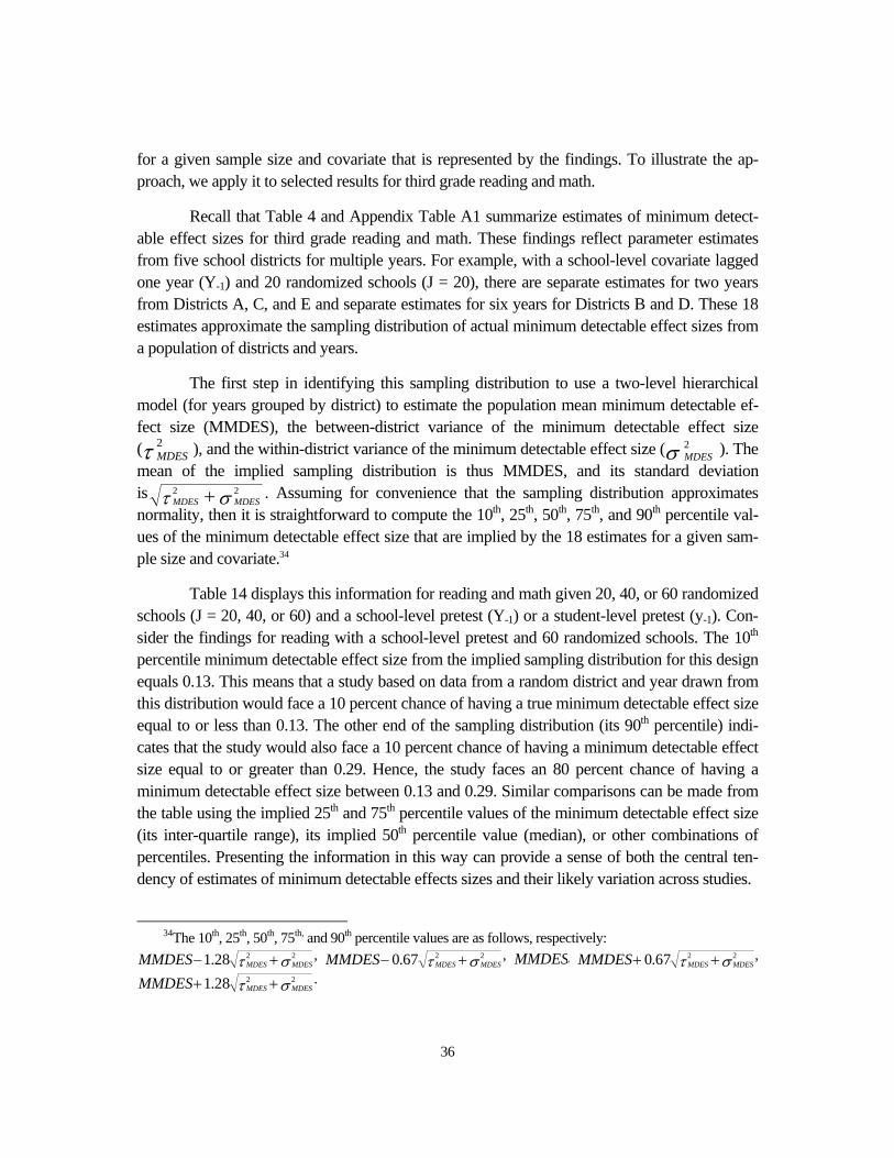
36
for a given sample size and covariate that is represented by the findings. To illustrate the ap-proach, we apply it to selected results for third grade reading and math.
Recall that Table 4 and Appendix Table A1 summarize estimates of minimum detect-able effect sizes for third grade reading and math. These findings reflect parameter estimates from five school districts for multiple years. For example, with a school-level covariate lagged one year (Y-1) and 20 randomized schools (J = 20), there are separate estimates for two years from Districts A, C, and E and separate estimates for six years for Districts B and D. These 18 estimates approximate the sampling distribution of actual minimum detectable effect sizes from a population of districts and years.
The first step in identifying this sampling distribution to use a two-level hierarchical model (for years grouped by district) to estimate the population mean minimum detectable ef-fect size (MMDES), the between-district variance of the minimum detectable effect size (τ 2
MDES ), and the within-district variance of the minimum detectable effect size (σ 2MDES ). The
mean of the implied sampling distribution is thus MMDES, and its standard deviation is στ 22
MDESMDES + . Assuming for convenience that the sampling distribution approximates normality, then it is straightforward to compute the 10th, 25th, 50th, 75th, and 90th percentile val-ues of the minimum detectable effect size that are implied by the 18 estimates for a given sam-ple size and covariate.34
Table 14 displays this information for reading and math given 20, 40, or 60 randomized schools (J = 20, 40, or 60) and a school-level pretest (Y-1) or a student-level pretest (y-1). Con-sider the findings for reading with a school-level pretest and 60 randomized schools. The 10th percentile minimum detectable effect size from the implied sampling distribution for this design equals 0.13. This means that a study based on data from a random district and year drawn from this distribution would face a 10 percent chance of having a true minimum detectable effect size equal to or less than 0.13. The other end of the sampling distribution (its 90th percentile) indi-cates that the study would also face a 10 percent chance of having a minimum detectable effect size equal to or greater than 0.29. Hence, the study faces an 80 percent chance of having a minimum detectable effect size between 0.13 and 0.29. Similar comparisons can be made from the table using the implied 25th and 75th percentile values of the minimum detectable effect size (its inter-quartile range), its implied 50th percentile value (median), or other combinations of percentiles. Presenting the information in this way can provide a sense of both the central ten-dency of estimates of minimum detectable effects sizes and their likely variation across studies.
34The 10th, 25th, 50th, 75th, and 90th percentile values are as follows, respectively:
στ 2228.1 MDESMDESMMDES +− , στ 2267.0 MDESMDESMMDES +− , MMDES, στ 2267.0 MDESMDESMMDES ++ ,
στ 2228.1 MDESMDESMMDES ++ .

37
Next Steps Previous research has established that adding a covariate adjustment — especially for
pretests — to a cluster-randomized study can often markedly improve its precision. The present paper presents a framework for exploring this process by identifying the three empirical pa-rameters (ρ, R2
C, and R2I) that determine precision when a covariate is used. In addition, the pa-
per begins to develop a systematic inventory of values for these parameters when the unit of random assignment is an elementary school, middle school, or high school and the outcome of interest is student achievement. There are three important directions in which to expand this research: to additional school districts, to other types of educational outcomes, and to other units of randomization.
Current estimates of ρ, R2C, and R2
I for student achievement measures clustered within schools are available for only a few school districts. Thus replication of these estimates for other districts is necessary to more fully understand their distribution across districts, years, grades, sub-jects, and sub-samples of schools. Perhaps the best source of this additional information in the next several years is the series of large-scale, multi-site, school-randomized studies currently being sponsored by the U.S. Department of Education’s Institute of Educational Sciences. Hence, it is important these studies report the values of ρ, R2
C, and R2I that underlie their findings. Another
potentially valuable source of such information is studies that could be commissioned using ex-tensive data that now exist in several states for individual student outcomes at all schools.35
A second important direction in which to expand the present analysis is to replicate it for other types of educational outcomes. For example, high school reforms often focus on improving rates of student attendance, promotion, credit accumulation, and graduation (as well as their per-formance on standardized tests). Thus knowledge of the intra-class correlations and predictive power of covariates for these outcome measures could be invaluable for designing evaluations of these reforms. In addition, some educational initiatives are designed to improve social and emo-tional outcomes for students (e.g., Aber, et al., 1999), so knowledge of the empirical parameters for these outcomes is important for designing future evaluations of such initiatives.
A third important direction in which to expand the present analysis is to replicate it for other units of randomization. For example, randomizing classrooms within schools can provide much greater precision than randomizing schools because multiple classrooms would be ran-domized per school. Thus, for educational interventions where it is logistically and politically feasible to randomize at this lower level of aggregation and for which it is possible to prevent “spillovers” between treatment and control classrooms, this approach could greatly reduce the
35See Bifulco and Ladd (2005) for a description of these data for North Carolina and Hanushek, Kain, and
Rivkin (2001) for a description of these data for Texas.

38
number of schools needed (and thus costs) of evaluations. However, little is known about ρ, R2
C, and R2I for student outcomes clustered within classrooms within schools.36
In addition, there is a large and growing interest in evaluating educational programs that take place in settings other than schools, such as child care centers (especially Head Start cen-ters), after-school programs, or pre-school programs. Thus, knowledge of the planning parame-ters for the relevant outcome measures and units of randomization for these studies is also an important needed addition to the current empirical repertoire.37
It is clear then that although recent advances in cluster-randomized studies for measur-ing the impacts of educational interventions have been considerable, there is much more to be learned about how to improve these designs. And it is equally clear what some of the next steps should be for informing these improvements.
36Schochet (2005) presents an estimate of 0.16 for the intra-class correlation of student test scores within
classrooms within schools based on data for low-income schools from two evaluation studies. 37Schochet (2005) presents estimates of these parameters for pre-schools.

39
References
Aber, Larry J., et al. 1999. “Teaching Conflict Resolution: An Effective School-Based Approach to Violence Prevention.” Report submitted to the National Center for Children in Poverty. New York: Columbia University.
Bifulco, Robert, and Helen F. Ladd. 2005. “The Impacts of Charter Schools on Student Achievement: Evidence from North Carolina.” Working Paper. Storrs: University of Connecticut, April 15.
Bloom, Howard S. 2005. “Randomizing Groups to Evaluate Place-Based Programs.” In Howard S. Bloom (ed.), Learning More from Social Experiments: Evolving Analytic Approaches. New York: Russell Sage Foundation.
Bloom, Howard S. 1995. “Minimum Detectable Effects: A Simple Way to Report the Statistical Power of Experimental Designs.” Evaluation Review 19(5): 547-56.
Bloom, Howard S., and Mark W. Lipsey. 2005. “Project on Uses and Abuses of Effect Size Meas-ures: Introduction to the Issues.” Powerpoint Presentation to U.S Department of Education, July 28. New York: MDRC.
Bloom, Howard S., Johannes M. Bos, and Suk-Won Lee. 1999. “Using Cluster Random Assign-ment to Measure Program Impacts: Statistical Implications for the Evaluation of Education Pro-grams.” Evaluation Review 23(4): 445-69.
Cohen, Jacob. 1977. Statistical Power Analysis for the Behavioral Sciences. New York: Academic Press.
Donner, Allan, and Neil Klar. 2000. Design and Analysis of Cluster Randomization Trials in Health Research. London: Arnold.
Feng, Ziding, Paula Diehr, Yutaka Yasui, Brent Evans, Shirley Beresford, and Thomas D. Koepsell. 1999. “Explaining Community-Level Variance in Group Randomized Trials.” Statistics in Medicine 18: 539-56.
Frison, Lars, and Stuart J. Pocock. 1992. “Repeated Measures in Clinical Trials: Analysis Using Mean Summary Statistics and Its Implications for Design.” Statistics in Medicine 11: 1685-1704.
Gail, Mitchell H., Steven D. Mark, Raymond J. Carroll, Sylvan B. Green, and David Pee. 1996. “On Design Considerations and Randomization-Based Inference for Community Intervention Tri-als.” Statistics in Medicine 15: 1069-92.
Gargani, John, and Thomas D. Cook. Forthcoming. “How Many Schools? Limits of the Conven-tional Wisdom About Sample Size Requirements for Cluster Randomized Trials.” Journal of the American Academy of Political and Social Science.
Hanushek, Eric A., John F. Kain, and Steven. G. Rivkin. 2001. “Disruption Versus Tiebout Im-provement: The Costs and Benefits of Switching Schools.” Working Paper No. 8479. New York: National Bureau of Economic Research.

40
Hedberg, Eric C., Rafael Santana, and Larry Hedges. 2004. “The Variance Structure of Academic Achievement in America.” Presentation to the 2004 Annual Meeting of the American Educa-tional Research Association.
Janega, Jessica B., David M. Murray, Sherri P. Varnell, Jonathan L. Blitstein, Amanda S. Birnbaum, and Leslie A. Lytle. 2004. “Assessing Intervention Effects in a School-Based Nutrition Inter-vention Trial: Which Analytic Model Is Most Powerful?” Health Education and Behavior 31(6): 756-74.
Kane, Thomas. 2004. “The Impact of After-School Programs: Interpreting the Results of Four Re-cent Evaluations.” New York: William T. Grant Foundation.
Lipsey, Mark W. 1990. Design Sensitivity: Statistical Power for Experimental Research. Newbury Park, CA: Sage Publications.
Martin, Donald C., Paula Diehr, Edward B. Perrin, and Thomas D. Koepsell. 1993. “The Effect of Matching on the Power of Randomized Community Intervention Studies.” Statistics in Medi-cine 12: 329-38.
Murray, David M. 1998. Design and Analysis of Group-Randomized Trials. New York: Oxford University Press.
Murray, David M., and Jonathan L. Blitstein. 2003. “Methods to Reduce the Impact of Intraclass Correlation in Group-Randomized Trials.” Evaluation Review 27(1): 79-103.
Murray, David, and Brian Short. 1995. “Intra-Class Correlation Among Measures Related to Alco-hol Use by Young Adults: Estimates, Correlates and Applications in Intervention Studies.” Journal of Studies on Alcohol 56(6): 681-94.
National Center for Education Statistics. 1997. “Reading and Mathematics Achievement Growth in High School.” Issue brief 98-038. Washington, DC: U.S. Department of Education.
Nye, Barbara, Larry V. Hedges, and Spyros Konstantopoulos. 1999. “The Long-Term Effects of Small Classes: A Five-Year Follow-Up of the Tennessee Class Size Experiment.” Educational Evaluation and Policy Analysis 21(2): 127-42.
Raudenbush, Stephen W. 1997. “Statistical Analysis and Optimal Design for Group Randomized Trials.” Psychological Methods 2(2): 173-85.
Raudenbush, Stephen W., Andres Martinez, and Jessaca Spybrook. 2005. “Strategies for Improving Precision in Group-Randomized Experiments.” New York: William T. Grant Foundation.
Raudenbush, Stephen W., and Xiao-Feng Liu. 2001. “Effects of Study Duration, Frequency of Ob-servation, and Sample Size on Power in Studies of Group Differences in Polynomial Change.” Psychological Methods 6(4): 387-401.
Schochet, Peter A. 2005. “Statistical Power for Random Assignment Evaluations of Education Pro-grams.” Princeton, NJ: Mathematica Policy Research.
Siddiqui, Ohidul, Donald Hedeker, Brian R. Flay, and Frank B. Hu. 1996. “Intraclass Correlation Estimates in a School-based Smoking Prevention Study: Outcome and Mediating Variables, by Sex and Ethnicity.” American Journal of Epidemiology 144(4): 425-33.

41
Singer, Judith D., and John B. Willett. 2003. Applied Longitudinal Data Analysis: Modeling Change and Event Occurrence. New York: Oxford University Press.
Ukoumunne, O. C., M. C. Gulliford, S. Chinn, J. A. C. Sterne, and P. F. J. Burney. 1999. “Methods for Evaluating Area-Wide and Organisation-Based Interventions in Health and Health Care: A Systematic Review.” Health Technology Assessment 3(5): 1-99.


Report Tables


45
Table 1
How Minimum Detectable Effect Size Varies with ρ, R2C, and R2
I
(Given J = 40, n = 60, and P = 0.5)
0.0 0.2 0.4 0.6 0.8
0.0 0.31 0.28 0.25 0.21 0.170.2 0.30 0.28 0.24 0.21 0.160.4 0.30 0.27 0.24 0.20 0.150.6 0.30 0.27 0.23 0.20 0.150.8 0.29 0.26 0.23 0.19 0.14
0.0 0.37 0.33 0.29 0.25 0.190.2 0.37 0.33 0.29 0.24 0.190.4 0.36 0.33 0.29 0.24 0.180.6 0.36 0.32 0.28 0.23 0.170.8 0.36 0.32 0.28 0.23 0.16
0.0 0.42 0.38 0.33 0.28 0.210.2 0.42 0.38 0.33 0.27 0.200.4 0.42 0.37 0.33 0.27 0.200.6 0.41 0.37 0.32 0.27 0.190.8 0.41 0.37 0.32 0.26 0.19
Using Covariates to Improve Precision
ρ = 0.2
R2I
R2C
ρ = 0.10
ρ = 0.15
NOTE: Minimum detectable effects are defined for 80 percent power, 0.05 significance, and a two-tail test. Multiplying them by 0.88 creates their counterparts for a one-tail test.

46
Using Covariates to Improve Precision
Table 2
Research Design Questions Addressed by the Present Analysis
Core Questions
1. How precise are estimates of intervention effects on student achievement for studies that randomize schools and control statistically for a pretest? How does the answer to this question differ for school-level versus student-level pretests?
2. By how much does precision vary across follow-up years as the gap in time between baseline and follow-up test results increases?
3. By how much does precision differ for reading and math outcomes? 4. By how much does precision differ for elementary schools, middle schools, or high
schools? 5. By how much does precision vary across school districts? 6. By how much does precision vary across years in the same school district?
Further Questions
1. By how much is precision improved through the addition of a pretest for a second baseline year?
2. By how much is precision improved through the combined use of a school-level and a student-level pretest?
3. How much precision exists if demographic characteristics only are used as covariates? 4. By how much is precision improved if demographic characteristics are added to a
baseline pretest as covariates? 5. By how much is precision reduced if the test used to measure baseline outcomes differs
from that used to measure follow-up outcomes? 6. How is precision affected if the sample of schools is limited to those with high
concentrations of students from low-income families (who receive subsidized meals) during the baseline period?
7. How is precision affected if the sample of schools is limited to those with especially poor student performance during the baseline period?

47
A B C D EElementary schools (Grade 3)
Average number of students 75 57 69 64 66
Average number of schools 68 88 168 48 25
Average student age 8 8 8 8 NA
Student race/ethnicity (%)Black 89 59 42 72 NAWhite 7 36 10 6 NAHispanic 3 2 45 21 NAAsian 1 2 3 0 NAOther 0 0 0 1 NA
Student gender (%)Male 51 51 51 49 NAFemale 49 49 49 51 NA
Low-income students (%) 79 66 41 NA NA
Middle schools (Grade 8)Average number of students 196 NA 297 NA NA
Average number of schools 17 NA 41 NA NA
Average student age 13 NA 13 NA NA
Student race/ethnicity (%)Black 93 NA 35 NA NAWhite 4 NA 8 NA NAHispanic 2 NA 54 NA NAAsian 1 NA 3 NA NAOther 0 NA 0 NA NA
NAStudent gender (%)
Male 48 NA 50 NA NAFemale 52 NA 50 NA NA
Low-income students (%) 68 NA 38 NA NA
Using Covariates to Improve Precision
Table 3
School and Student Characteristics by Grade and District
Grade and characteristicsDistrict
(continued)

48
A B C D E
High schools (Grade 10)Average number of students 234 NA 269 NA NA
Average number of schools 11 NA 32 NA NA
Average student age 15 NA 16 NA NA
Student race/ethnicity (%)Black 93 NA 40 NA NAWhite 5 NA 10 NA NAHispanic 1 NA 47 NA NAAsian 1 NA 3 NA NAOther 0 NA 0 NA NA
Student gender (%)Male 46 NA 49 NA NAFemale 54 NA 51 NA NA
Low-income students (%) 61 NA 31 NA NA
Grade and characteristicsDistrict
Table 3 (continued)
NOTES: Low-income students are defined as those students receiving free lunch, except in District B where they are defined as those identified by the district as being economically disadvantaged.
District A's 3rd and 8th grade averages are based on the 1998-99 and 1999-00 school years. The 10th grade averages are based on the 1996-97 and 1997-98 school years.
District B's 3rd grade averages are based on the 1997-98 through 2002-03 school years. The 10th grade averages are based on the 2000-01 and 2001-02 school years.
District C's averages are based on the 2001-02 and 2002-03 school years.
District D's averages are based on the 1993-94 through 1998-99 school years. Data on free lunch status was not available to identify low-income students.

49
Table 4
Grade 3 Reading
Minimum Detectable Effect Size (MDES) by Number of Randomized Schools (J) and Single Covariate
A B C D E Mean
No covariate 0.61 0.54 0.59 0.63 0.47 0.57 Y-1 0.52 0.29 0.33 0.46 0.27 0.37 Y-2 0.54 0.35 0.38 0.52 0.24 0.40 Y-3 NA 0.36 0.39 0.55 NA (0.43) y-1 0.52 0.29 0.32 0.53 0.25 0.38 y-2 0.55 NA 0.38 NA 0.25 (0.39) y-3 NA NA NA NA NA NA
No covariate 0.42 0.37 0.41 0.44 0.33 0.39 Y-1 0.36 0.20 0.23 0.31 0.19 0.26 Y-2 0.37 0.24 0.26 0.36 0.17 0.28 Y-3 NA 0.24 0.27 0.38 NA (0.30) y-1 0.35 0.20 0.22 0.36 0.18 0.26 y-2 0.38 NA 0.26 NA 0.18 (0.27) y-3 NA NA NA NA NA NA
No covariate 0.34 0.30 0.33 0.35 0.27 0.32 Y-1 0.29 0.16 0.18 0.25 0.16 0.21 Y-2 0.30 0.19 0.21 0.29 0.14 0.23 Y-3 NA 0.20 0.22 0.30 NA (0.24) y-1 0.29 0.16 0.18 0.29 0.14 0.21 y-2 0.31 NA 0.21 NA 0.15 (0.22) y-3 NA NA NA NA NA NA
Using Covariates to Improve Precision
MDES(J=40)
MDES(J=60)
CovariateFindings for District
MDES(J=20)
NOTES: In the last column, means in parenthesis indicate that the reported values do not include the values from all five districts. Y-1, Y-2, and Y-3 are mean school scores for the same grade lagged one, two, and three years, respectively. y-1, y-2, and y-3 are individual student scores lagged one, two, and three years, respectively. Findings reflect: statistical significance of 0.05, statistical power of 0.80, a two-tail hypothesis test, 60 students per school, and a balanced (50/50) allocation of schools to treatment and control status. Entries are computed using the mean of the corresponding district-level parameters. See Table 7 for these parameters.
District A's outcomes are based on tests administered in spring 1999 and spring 2000, with 77 students per school and 68 schools, on average. District B's outcomes are based on tests administered in spring 1998 through spring 2003, with 57 students per school and 89 schools, on average. District C's outcomes are based on tests administered in spring 2002 and spring 2003, with 69 students per school and 169 schools, on average. District D's outcomes are based on tests administered in spring 1994 through spring 1999, with 65 students per school and 48 schools, on average. District E's outcomes are taken from Table 4 of Bloom, Bos, and Lee (1999).

50
Table 5
Grade 3 Reading
Minimum Detectable Effect Size for 40 Randomized Schools withAlternative Samples of Schools and Covariates
(Excluding District E)
A B C D MeanAll schoolsNo covariate 0.42 0.37 0.41 0.44 0.41 Y-1 0.36 0.20 0.23 0.31 0.27 Y-1,Y-2 0.35 0.19 0.22 0.31 0.27 y-1 0.35 0.20 0.22 0.36 0.28 y-1,y-2 0.35 NA 0.21 NA (0.28) Y-1,y-1 0.34 0.17 0.19 0.31 0.25 Z-1 0.35 0.22 0.28 0.32 0.29 z-1 0.37 0.24 0.28 0.34 0.31 X 0.35 0.29 0.27 NA (0.31) X,Y-1 0.32 0.19 0.21 NA (0.24) X,y-1 0.33 0.19 0.20 NA (0.24)Low-income schools Y-1 0.36 0.21 0.26 NA (0.27) y-1 0.36 0.20 0.24 NA (0.26)Low-achieving schools Y-1 0.34 0.22 0.23 0.30 0.27 y-1 0.34 0.21 0.19 0.35 0.27
(continued)
School sample and covariatesFindings for District
Using Covariates to Improve Precision
NOTES: In the last column, means in parenthesis indicate that the reported values do not include the values from all four districts.Y-1 and Y-2 are mean school scores for the same grade lagged one and two years, respectively. y-1
and y-2 are individual student scores lagged one and two years, respectively. Z-1 and z-1 are mean school scores and individual scores in the previous year for a different test (with a math test as the pretest for reading outcomes and a reading test as the pretest for math outcomes). X is a vector of demographic characteristics, which differs across districts. Low-income schools are defined as those whose average proportion of students eligible for free lunch exceeds the district average. Low-achieving schools in the district are defined as those whose average combined sum of reading and math pretest scores were lower than the corresponding district average. Findings reflect: statistical significance of 0.05, statistical power of 0.80, a two-tail hypothesis test, 60 students per school, and a balanced (50/50) allocation of schools to treatment and control status.
District A's outcomes are based on tests administered in spring 1999 and spring 2000, with 77 students per school and 68 schools, on average. The low-income sample outcomes are based on data consisting of 76 students and 49 schools, on average. The low-achieving sample outcomes are based on data consisting of 71 students and 35 schools, on average.

51
Table 5 (continued)
District B's outcomes are based on tests administered in spring 1998 through spring 2003, with 57 students per school and 89 schools, on average. Low-income schools in District B are defined as those identified by the district as being economically disadvantaged. The low-income sample outcomes are based on data consisting of 58 students and 48 schools, on average. The low-achieving sample outcomes are based on data consisting of 57 students and 43 schools, on average.
District C's outcomes are based on tests administered in spring 2002 and spring 2003, with 69 students per school and 169 schools, on average. The low-income sample outcomes are based on data consisting of 62 students per school and 129 schools, on average. The low-achieving sample outcomes are based on data consisting of 59 students per school and 76 schools, on average.
District D's outcomes are based on tests administered in spring 1994 through spring 1999, with 65 students per school and 48 schools, on average. The low-achieving sample outcomes are based on data consisting of 61 students per school and 23 schools, on average. Data on free lunch status was not available to identify low-income schools.

52
(min, max) (min, max) (min, max) (min, max) (min, max)All schools Y-1 (0.34, 0.37) (0.18, 0.22) (0.21, 0.24) (0.27, 0.35) (0.18, 0.20) y-1 (0.34, 0.37) (0.17, 0.22) (0.19, 0.25) (0.33, 0.44) (0.16, 0.19)Low-income schools Y-1 (0.33, 0.39) (0.19, 0.24) (0.24, 0.27) NA NA NA NA y-1 (0.34, 0.37) (0.18, 0.23) (0.21, 0.27) NA NA NA NALow-achieving schools Y-1 (0.31, 0.37) (0.20, 0.25) (0.22, 0.24) (0.21, 0.36) NA NA y-1 (0.32, 0.35) (0.18, 0.25) (0.18, 0.20) (0.25, 0.45) NA NA
School sample and covariateFindings for District
A B C D E
Alternative Samples of Schools and Selected Covariates
Using Covariates to Improve Precision
Table 6
Minimum Detectable Effect Size Ranges for 40 Randomized Schools with
Grade 3 Reading
NOTES: Y-1 is the mean school score for the same grade lagged one year, and y-1is the individual student score lagged one year. Low-income schools are defined as those whose average proportion of students eligible for free lunch exceeds the district average. Low-achieving schools in the district are defined as those whose average combined sum of reading and math pretest scores were lower than the corresponding district average. Findings reflect: statistical significance of 0.05, statistical power of 0.80, a two-tail hypothesis test, 60 students per school, anda balanced (50/50) allocation of schools to treatment and control status.
District A's outcomes are based on tests administered in spring 1999 and spring 2000, with 77 students per school and 68 schools, on average. The low-income sample outcomes are based on data consisting of 76 students and 49 schools, on average. The low-achieving sample outcomes are based on data consisting of 71 students and 35 schools,on average.
District B's outcomes are based on tests administered in spring 1998 through spring 2003, with 57 students per schooand 89 schools, on average. Low-income schools in District B are defined as those identified by the district as being economically disadvantaged. The low-income sample outcomes are based on data consisting of 58 students and 48 schools, on average. The low-achieving sample outcomes are based on data consisting of 57 students and 43 schools,on average.
District C's outcomes are based on tests administered in spring 2002 and spring 2003, with 69 students per school and169 schools, on average. The low-income sample outcomes are based on data consisting of 62 students per school and 129 schools, on average. The low-achieving sample outcomes are based on data consisting of 59 students per school and 76 schools, on average.
District D's outcomes are based on tests administered in spring 1994 through spring 1999, with 65 students per schooand 48 schools, on average. The low-achieving sample outcomes are based on data consisting of 61 students per school and 23 schools, on average. Data on free lunch status was not available to identify low-income schools.
District E's outcomes are taken from Table 4 of Bloom, Bos, and Lee (1999).

Table 7
Grade 3 Reading
Parameter Values for Selected Covariates
R2C R2
I R2C R2
I R2C R2
I R2C R2
I R2C R2
I
Y-1 0.31 0.00 0.77 0.00 0.74 0.00 0.51 0.00 0.75 0.00Y-2 0.25 0.00 0.63 0.00 0.64 0.00 0.35 0.00 0.81 0.00Y-3 NA NA 0.62 0.00 0.60 0.00 0.27 0.00 NA NAY-1, Y-2 0.35 0.00 0.79 0.00 0.76 0.00 0.53 0.00 0.89 0.00Y-2, Y-3 NA NA 0.71 0.00 0.68 0.00 0.39 0.00 NA NA
y-1 0.30 0.22 0.73 0.40 0.73 0.46 0.31 0.30 0.73 0.52y-2 0.18 0.12 NA NA 0.62 0.30 NA NA 0.73 0.31y-3 NA NA NA NA NA NA NA NA NA NAy-1, y-2 0.33 0.26 NA NA 0.75 0.48 NA NA 0.78 0.54y-2, y-3 NA NA NA NA NA NA NA NA NA NA
Y-1, y-1 0.37 0.22 0.83 0.40 0.80 0.46 0.51 0.30 NA NAZ-1 0.34 0.00 0.71 0.00 0.58 0.00 0.48 0.00 NA NAz-1 0.25 0.15 0.60 0.25 0.56 0.28 0.39 0.20 NA NAX 0.30 0.08 0.40 0.07 0.58 0.23 NA NA NA NAX, Y-1 0.43 0.08 0.79 0.07 0.78 0.23 NA NA NA NAX, y-1 0.40 0.25 0.78 0.42 0.77 0.50 NA NA NA NA
(continued)
0.19 0.22 0.16
CovariatesParameters for District
A B C D E
Using Covariates to Improve Precision
Other covariates
Proportion of variance reduced (R2C and R2
I)
School-level pretests only
Student-level pretests only
Intra-class correlation with no covariates (ρ)0.20 0.15
53

Table 7 (continued)
NOTES: Y-1, Y-2, and Y-3 are mean school scores for the same grade lagged one, two, and three years, respectively. y-1, y-2, and y-3 are individual student scores lagged one, two, and three years, respectively. X is a vector of demographic characteristics, which differs across districts. Z-1 and z-1 are mean school scores and individual scores in the previous year for a different test (with a math test as the pretest for reading outcomes and a reading test as the pretest for math outcomes). R2
C and R2I are the average proportion of the school-level variance and the student-level variance reduced by the covariates, respectively.
The averages are computed as the mean of the corresponding district-level parameters. Nonzero estimates for R2I with school-level covariates only are set
equal to zero. See text for more details.
District A's outcomes are based on tests administered in spring 1999 and spring 2000, with 77 students per school and 68 schools, on average. District B's outcomes are based on tests administered in spring 1998 through spring 2003, with 57 students per school and 89 schools, on average. District C's outcomes are based on tests administered in spring 2002 and spring 2003, with 69 students per school and 169 schools, on average. District D's outcomes are based on tests administered in spring 1994 through spring 1999, with 65 students per school and 48 schools, on average. District E's outcomes are taken from unpublished tables of Bloom, Bos, and Lee (1999).
54
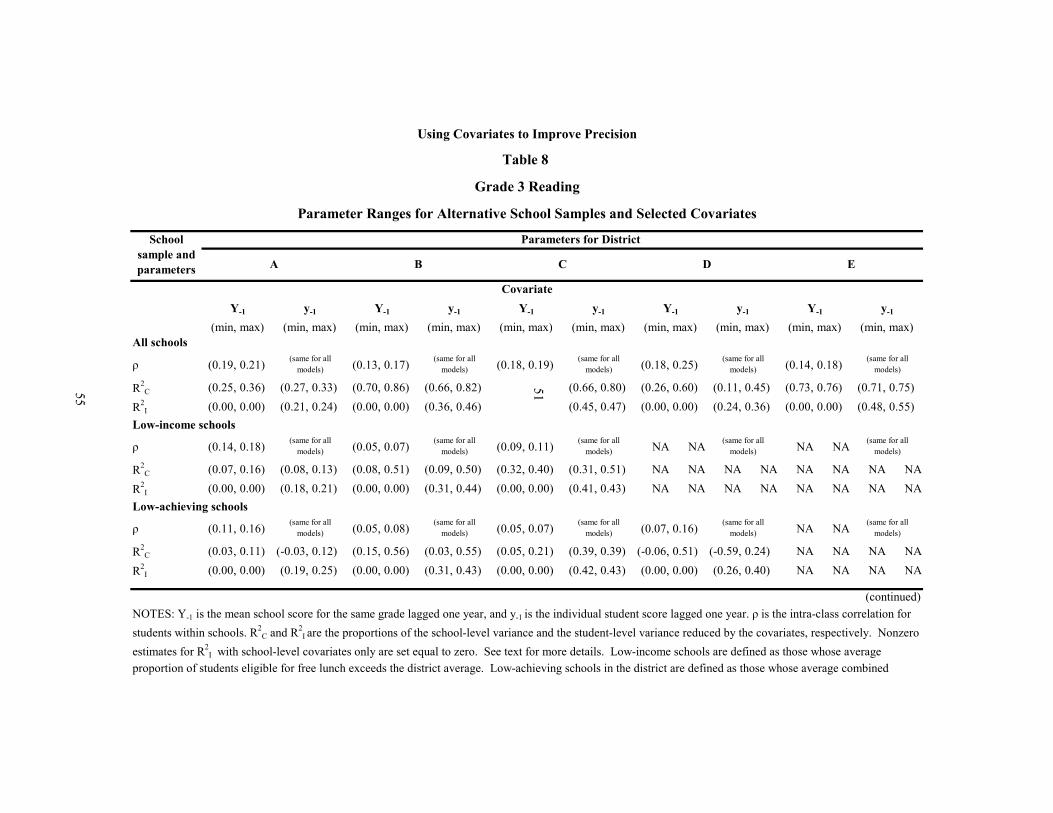
Table 8
Grade 3 Reading
Parameter Ranges for Alternative School Samples and Selected Covariates
(min, max) (min, max) (min, max) (min, max) (min, max) (min, max) (min, max) (min, max) (min, max) (min, max)All schools
ρ (0.19, 0.21) (0.13, 0.17) (0.18, 0.19) (0.18, 0.25) (0.14, 0.18)
R2C (0.25, 0.36) (0.27, 0.33) (0.70, 0.86) (0.66, 0.82) (0.71, 0.78) (0.66, 0.80) (0.26, 0.60) (0.11, 0.45) (0.73, 0.76) (0.71, 0.75)
R2I (0.00, 0.00) (0.21, 0.24) (0.00, 0.00) (0.36, 0.46) (0.00, 0.00) (0.45, 0.47) (0.00, 0.00) (0.24, 0.36) (0.00, 0.00) (0.48, 0.55)
ρ (0.14, 0.18) (0.05, 0.07) (0.09, 0.11) NA NA NA NA
R2C (0.07, 0.16) (0.08, 0.13) (0.08, 0.51) (0.09, 0.50) (0.32, 0.40) (0.31, 0.51) NA NA NA NA NA NA NA NA
R2I (0.00, 0.00) (0.18, 0.21) (0.00, 0.00) (0.31, 0.44) (0.00, 0.00) (0.41, 0.43) NA NA NA NA NA NA NA NA
ρ (0.11, 0.16) (0.05, 0.08) (0.05, 0.07) (0.07, 0.16) NA NA
R2C (0.03, 0.11) (-0.03, 0.12) (0.15, 0.56) (0.03, 0.55) (0.05, 0.21) (0.39, 0.39) (-0.06, 0.51) (-0.59, 0.24) NA NA NA NA
R2I (0.00, 0.00) (0.19, 0.25) (0.00, 0.00) (0.31, 0.43) (0.00, 0.00) (0.42, 0.43) (0.00, 0.00) (0.26, 0.40) NA NA NA NA
(continued)
Y-1
School sample and parameters
Parameters for District
A B C D E
(same for all models)
CovariateY-1 y-1 Y-1 y-1 Y-1 y-1 Y-1 y-1
(same for all models)
(same for all models)
Low-achieving schools
Low-income schools(same for all
models)
(same for all models)
(same for all models)
(same for all models)
(same for all models)
(same for all models)
(same for all models)
Using Covariates to Improve Precision
(same for all models)
(same for all models)
y-1
(same for all models)
(same for all models)
(same for all models)
NOTES: Y-1 is the mean school score for the same grade lagged one year, and y-1 is the individual student score lagged one year. ρ is the intra-class correlation for students within schools. R2
C and R2I are the proportions of the school-level variance and the student-level variance reduced by the covariates, respectively. Nonzero
estimates for R2I with school-level covariates only are set equal to zero. See text for more details. Low-income schools are defined as those whose average
proportion of students eligible for free lunch exceeds the district average. Low-achieving schools in the district are defined as those whose average combined
51 55

Table 8 (continued)sum of reading and math pretest scores were lower than the corresponding district average.
District A's outcomes are based on tests administered in spring 1999 and spring 2000, with 77 students per school and 68 schools, on average. The low-income sample outcomes are based on data consisting of 76 students and 49 schools, on average. The low-achieving sample outcomes are based on data consisting of 71 students and 35 schools, on average.
District B's outcomes are based on tests administered in spring 1998 through spring 2003, with 57 students per school and 89 schools, on average. Low-income schools in District B are defined as those identified by the district as being economically disadvantaged. The low-income sample outcomes are based on data consisting of 58 students and 48 schools, on average. The low-achieving sample outcomes are based on data consisting of 57 students and 43 schools, on average.
District C's outcomes are based on tests administered in spring 2002 and spring 2003, with 69 students per school and 169 schools, on average. The low-income sample outcomes are based on data consisting of 62 students per school and 129 schools, on average. The low-achieving sample outcomes are based on data consisting of 59 students per school and 76 schools, on average.
District D's outcomes are based on tests administered in spring 1994 through spring 1999, with 65 students per school and 48 schools, on average. The low-achieving sample outcomes are based on data consisting of 61 students per school and 23 schools, on average. Data on free lunch status was not available to identify low-income schools.
District E's outcomes are taken from unpublished tables of Bloom, Bos, and Lee (1999).
56

57
Table 9
Elementary School
Average Minimum Detectable Effect Size (MDES) by Number of Randomized Schools (J) and Single Covariate
Reading Math Reading Math
No covariate 0.57 0.58 0.56 0.57 Y-1 0.37 0.37 0.38 0.38 Y-2 0.40 0.42 0.40 0.41 Y-3 (0.43) (0.47) (0.36) (0.44) y-1 0.38 0.43 0.40 0.39 y-2 (0.39) (0.45) 0.36 0.38 y-3 NA NA (0.61) (0.50)
No covariate 0.39 0.40 0.38 0.39 Y-1 0.26 0.26 0.26 0.26 Y-2 0.28 0.29 0.28 0.28 Y-3 (0.30) (0.32) (0.25) (0.30) y-1 0.26 0.30 0.27 0.27 y-2 (0.27) (0.31) 0.25 0.27 y-3 NA NA (0.42) (0.34)
No covariate 0.32 0.32 0.31 0.32 Y-1 0.21 0.21 0.21 0.21 Y-2 0.23 0.23 0.22 0.23 Y-3 (0.24) (0.26) (0.20) (0.24) y-1 0.21 0.24 0.22 0.22 y-2 (0.22) (0.25) 0.20 0.22 y-3 NA NA (0.34) (0.28)
Using Covariates to Improve Precision
MDES(J=20)
MDES(J=40)
MDES(J=60)
CovariateFindings by Grade and Subject
Third Grade Fifth Grade
NOTES: Means in parenthesis indicate that the reported values do not include the values from all districts. Y-1, Y-2, and Y-3 are mean school scores for the same grade lagged one, two, and three years, respectively. y-1, y-2, and y-3 are individual student scores lagged one, two, and three years, respectively. Findings reflect: statistical significance of 0.05, statistical power of 0.80, a two-tail hypothesis test, 60 students per school, and a balanced (50/50) allocation of schools to treatment and control status. Entries are computed using the mean of the corresponding district-level outcomes. See Table 4 for these outcomes and sample sizes for third grade reading and Appendix Tables A1, A6, and A11 for third grade math, fifth grade reading, and fifth grade math, respectively.

58
Table 10
Elementary School
Average Minimum Detectable Effect Size for 40 Randomized Schools withAlternative Samples of Schools and Covariates
Reading Math Reading Math
All schoolsNo covariate 0.41 0.41 0.42 0.41 Y-1 0.27 0.28 0.29 0.28 Y-1,Y-2 0.27 0.27 0.28 0.26 y-1 0.28 0.30 0.33 0.30 y-1,y-2 (0.28) (0.29) 0.28 0.26 Y-1,y-1 0.25 0.26 0.30 0.27 Z-1 0.29 0.28 0.32 0.28 z-1 0.31 0.30 0.33 0.30 X (0.31) (0.31) 0.32 0.31 X,Y-1 (0.24) (0.24) 0.26 0.25 X,y-1 (0.24) (0.25) 0.31 0.28Low-income schools Y-1 (0.27) (0.27) 0.29 0.29 y-1 (0.26) (0.27) 0.31 0.32Low-achieving schools Y-1 0.27 0.28 0.30 0.30 y-1 0.27 0.30 0.35 0.34
Using Covariates to Improve Precision
School sample and covariatesFindings by Grade and Subject
Third Grade Fifth Grade
NOTES: Means in parenthesis indicate that the reported values do not include the values from all districts. Y-
1 and Y-2 are mean school scores for the same grade lagged one and two years, respectively. y-1, and y-2 are individual student scores lagged one and two years, respectively. Z-1 and z-1 are mean school scores and individual scores in the previous year for a different test (with a math test as the pretest for reading outcomes and a reading test as the pretest for math outcomes). X is a vector of demographic characteristics, which differs across districts. Low-income schools are defined as those whose average proportion of students eligible for free lunch exceeds the district average. Low-achieving schools in the district are defined as those whose average combined sum of reading and math pretest scores were lower than the corresponding district average. Findings reflect: statistical significance of 0.05, statistical power of 0.80, a two-tail hypothesis test, 60 students per school, and a balanced (50/50) allocation of schools to treatment and control status.

59
Table 11
Middle School and High School
Average Minimum Detectable Effect Size (MDES) by Number of Randomized Schools (J) and Single Covariate
Reading Math Reading Math
No covariate 0.61 0.61 0.62 0.58 Y-1 0.24 0.28 0.16 0.16 Y-2 0.30 0.35 0.24 0.21 Y-3 (0.28) 0.37 (0.26) (0.29) y-1 0.28 0.28 0.15 0.23 y-2 0.27 0.33 (0.25) 0.26 y-3 (0.25) 0.36 (0.25) (0.30)
No covariate 0.42 0.42 0.42 0.40 Y-1 0.17 0.19 0.11 0.11 Y-2 0.20 0.24 0.16 0.15 Y-3 (0.19) 0.25 (0.18) (0.20) y-1 0.19 0.19 0.10 0.15 y-2 0.19 0.22 (0.17) 0.18 y-3 (0.17) 0.24 (0.17) (0.21)
No covariate 0.34 0.34 0.34 0.32 Y-1 0.13 0.15 0.09 0.09 Y-2 0.16 0.20 0.13 0.12 Y-3 (0.15) 0.20 (0.14) (0.16) y-1 0.15 0.16 0.08 0.12 y-2 0.15 0.18 (0.14) 0.14 y-3 (0.14) 0.20 (0.14) (0.17)
Using Covariates to Improve Precision
MDES(J=20)
MDES(J=40)
MDES(J=60)
CovariateFindings by Grade and Subject
Eighth Grade Tenth Grade
NOTES: Means in parenthesis indicate that the reported values do not include the values from all districts. Y-1, Y-2, and Y-3 are mean school scores for the same grade lagged one, two, and three years, respectively. y-1, y-2, and y-3 are individual student scores lagged one, two, and three years, respectively. Findings reflect: statistical significance of 0.05, statistical power of 0.80, a two-tail hypothesis test, 250 students per school, and a balanced (50/50) allocation of schools to treatment and control status. Entries are computed using the mean of the corresponding district-level outcomes. See Appendix Tables A16, A21, A26, and A31 for these outcomes and sample sizes for eighth and tenth grade reading and math.
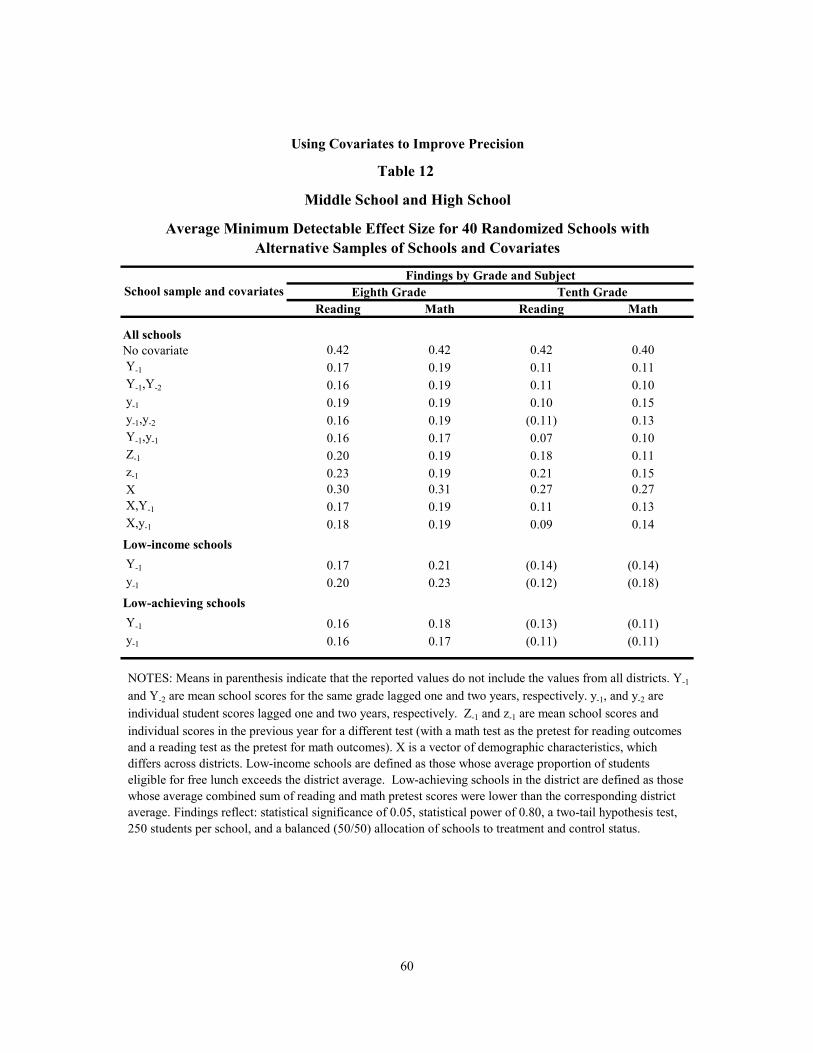
60
Table 12
Middle School and High School
Average Minimum Detectable Effect Size for 40 Randomized Schools withAlternative Samples of Schools and Covariates
Reading Math Reading Math
All schoolsNo covariate 0.42 0.42 0.42 0.40 Y-1 0.17 0.19 0.11 0.11 Y-1,Y-2 0.16 0.19 0.11 0.10 y-1 0.19 0.19 0.10 0.15 y-1,y-2 0.16 0.19 (0.11) 0.13 Y-1,y-1 0.16 0.17 0.07 0.10 Z-1 0.20 0.19 0.18 0.11 z-1 0.23 0.19 0.21 0.15 X 0.30 0.31 0.27 0.27 X,Y-1 0.17 0.19 0.11 0.13 X,y-1 0.18 0.19 0.09 0.14Low-income schools Y-1 0.17 0.21 (0.14) (0.14) y-1 0.20 0.23 (0.12) (0.18)Low-achieving schools Y-1 0.16 0.18 (0.13) (0.11) y-1 0.16 0.17 (0.11) (0.11)
Using Covariates to Improve Precision
School sample and covariatesFindings by Grade and Subject
Eighth Grade Tenth Grade
NOTES: Means in parenthesis indicate that the reported values do not include the values from all districts. Y-1
and Y-2 are mean school scores for the same grade lagged one and two years, respectively. y-1, and y-2 are individual student scores lagged one and two years, respectively. Z-1 and z-1 are mean school scores and individual scores in the previous year for a different test (with a math test as the pretest for reading outcomes and a reading test as the pretest for math outcomes). X is a vector of demographic characteristics, which differs across districts. Low-income schools are defined as those whose average proportion of students eligible for free lunch exceeds the district average. Low-achieving schools in the district are defined as those whose average combined sum of reading and math pretest scores were lower than the corresponding district average. Findings reflect: statistical significance of 0.05, statistical power of 0.80, a two-tail hypothesis test, 250 students per school, and a balanced (50/50) allocation of schools to treatment and control status.

61
Table 13
Mean Estimates of ρ and R2C
by Grade, Subject, and District
A B C D E
Third grade Reading 0.20 0.15 0.19 0.22 0.16 Math 0.20 0.17 0.17 0.23 0.18
Fifth grade Reading 0.25 0.15 0.20 NA 0.12 Math 0.20 0.19 0.17 NA 0.18
Eighth grade Reading 0.18 NA 0.23 NA NA Math 0.16 NA 0.27 NA NA
Tenth grade Reading 0.15 NA 0.29 NA NA Math 0.13 NA 0.25 NA NA
Third grade Reading 0.31 0.77 0.74 0.51 0.75 Math 0.54 0.71 0.61 0.48 0.82
Fifth grade Reading 0.33 0.50 0.81 NA 0.70 Math 0.47 0.54 0.66 NA 0.73
Eighth grade Reading 0.77 NA 0.91 NA NA Math 0.78 NA 0.83 NA NA
Tenth grade Reading 0.93 NA 0.95 NA NA Math 0.97 NA 0.91 NA NA
Estimates of R2C for Y-1
Using Covariates to Improve Precision
Grade and subject District
Estimates of ρ
NOTES: Y-1 is the mean school score for the same grade lagged one year. ρ is the intra-class correlation for students within schools. R2
C is the average proportion of the school cluster-level variance reduced by the covariate. The averages are computed as the mean of the corresponding district-level parameters.
District A's 3rd, 5th, and 8th grade averages are based on tests administered in spring 1999 and spring 2000. The 10th grade averages are tests administered in spring 1997 and spring 1998.
District B's 3rd grade averages are based on tests administered in spring 1998 through spring 2003. The 5th grade averages are based on tests administered in spring 1997. The 10th grade averages are based on tests administered in spring 2001 and spring 2002.
District C's 3rd, 5th, and 8th grade averages are based on tests administered in spring 2002 and spring 2003.
District D's 3rd grade averages are based on tests administered in spring 1994 through spring 1999.

62
10th 25th 50th 75th 90thPercentile Percentile Percentile Percentile Percentile
Covariate = Y-1
J = 20 0.23 0.29 0.36 0.43 0.50J = 40 0.16 0.21 0.26 0.31 0.35J = 60 0.13 0.17 0.21 0.25 0.29
Covariate = y-1
J = 20 0.20 0.28 0.37 0.46 0.54J = 40 0.14 0.20 0.26 0.32 0.38J = 60 0.12 0.16 0.21 0.27 0.31
Covariate = Y-1
J = 20 0.25 0.30 0.36 0.42 0.48J = 40 0.18 0.21 0.26 0.30 0.34J = 60 0.14 0.17 0.21 0.24 0.28
Covariate = y-1
J = 20 0.33 0.37 0.42 0.47 0.52J = 40 0.23 0.26 0.30 0.33 0.37J = 60 0.19 0.21 0.24 0.27 0.30
Using Covariates to Improve Precision
Third Grade Reading
Third Grade Math
Table 14
Percentile Values of Minimum Detectable Effect SizesImplied by Estimates for Third Grade Reading and Math
Covariate and sample size
NOTES: Y-1 is the mean school score for the same grade lagged one year, and y-1 is the individual student score lagged one year. Findings reflect statistical significance of 0.05, statistical power of 0.80, a two-tail hypothesis test, 60 students per school, and a balanced (50/50) allocation of schoools to treatment and control status. Findings are based on two years of data for Districts A, C, and E and six years of data for Districts B and D.

63
Appendix
Additional Detailed Findings by Grade and Subject
This appendix contains seven series of five tables each. A series of tables presents detailed findings for a specific grade and subject in the same format as Tables 4 – 8 for 3rd grade reading. The tables are numbered as follows.
3rd grade math Tables A1 – A5
5th grade reading Tables A6 – A10
5th grade math Tables A11 – A15
8th grade reading Tables A16 – A20
8th grade math Tables A21 – A25
10th grade reading Tables A26 – A30
10th grade math Tables A31 – A35

64
Appendix Table A1
Grade 3 Math
Minimum Detectable Effect Size (MDES) by Number of Randomized Schools (J) and Single Covariate
A B C D E Mean
No covariate 0.61 0.57 0.57 0.65 0.49 0.58 Y-1 0.42 0.34 0.38 0.48 0.25 0.37 Y-2 0.46 0.39 0.42 0.53 0.29 0.42 Y-3 0.46 0.42 0.43 0.56 NA (0.47) y-1 0.49 0.35 0.39 0.51 0.43 0.43 y-2 0.51 NA 0.43 NA 0.41 (0.45) y-3 NA NA NA NA NA NA
No covariate 0.42 0.39 0.39 0.45 0.35 0.40 Y-1 0.29 0.23 0.26 0.33 0.18 0.26 Y-2 0.32 0.27 0.29 0.37 0.21 0.29 Y-3 0.32 0.29 0.30 0.39 NA (0.32) y-1 0.34 0.24 0.26 0.35 0.31 0.30 y-2 0.35 NA 0.29 NA 0.29 (0.31) y-3 NA NA NA NA NA NA
No covariate 0.34 0.32 0.32 0.36 0.29 0.32 Y-1 0.24 0.19 0.21 0.27 0.14 0.21 Y-2 0.26 0.22 0.23 0.30 0.17 0.23 Y-3 0.26 0.23 0.24 0.31 NA (0.26) y-1 0.27 0.20 0.21 0.28 0.25 0.24 y-2 0.29 NA 0.24 NA 0.24 (0.25) y-3 NA NA NA NA NA NA
MDES(J=40)
MDES(J=60)
Using Covariates to Improve Precision
Covariate Findings for District
MDES(J=20)
NOTES: In the last column, means in parenthesis indicate that the reported values do not include the values from all five districts. Y-1, Y-2, and Y-3 are mean school scores for the same grade lagged one, two, and three years, respectively. y-1, y-2, and y-3 are individual student scores lagged one, two, and three years, respectively. Findings reflect: statistical significance of 0.05, statistical power of 0.80, a two-tail hypothesis test, 60 students per school, and a balanced (50/50) allocation of schools to treatment and control status. Entries are computed using the mean of the corresponding district-level parameters. See Appendix Table A4 for these parameters.
District A's outcomes are based on tests administered in spring 1999 and spring 2000, with 77 students per school and 68 schools, on average. District B's outcomes are based on tests administered in spring 1998 through spring 2003, with 57 students per school and 89 schools, on average. District C's outcomes are based on tests administered in spring 2002 and spring 2003, with 69 students per school and 169 schools, on average. District D's outcomes are based on tests administered in spring 1994 through spring 1999, with 65 students per school and 48 schools, on average. District E's outcomes are taken from Table 4 of Bloom, Bos, and Lee (1999).

65
Appendix Table A2
Grade 3 Math
Minimum Detectable Effect Size for 40 Randomized Schools with Alternative Samples of Schools and Covariates
(Excluding District E)
A B C D MeanAll schoolsNo covariate 0.42 0.39 0.39 0.45 0.41 Y-1 0.29 0.23 0.26 0.33 0.28 Y-1,Y-2 0.28 0.22 0.25 0.32 0.27 y-1 0.34 0.24 0.26 0.35 0.30 y-1,y-2 0.32 NA 0.25 NA (0.29) Y-1,y-1 0.29 0.21 0.25 0.31 0.26 Z-1 0.29 0.23 0.26 0.33 0.28 z-1 0.34 0.24 0.26 0.35 0.30 X 0.31 0.31 0.31 NA (0.31) X,Y-1 0.25 0.22 0.25 NA (0.24) X,y-1 0.28 0.23 0.25 NA (0.25)Low-income schools Y-1 0.28 0.25 0.27 NA (0.27) y-1 0.30 0.24 0.28 NA (0.27)Low-achieving schools Y-1 0.27 0.26 0.25 0.34 0.28 y-1 0.31 0.26 0.27 0.34 0.30
(continued)
School sample and covariates Findings for District
Using Covariates to Improve Precision
NOTES: In the last column, means in parenthesis indicate that the reported values do not include the values from all four districts. Y-1 and Y-2 are mean school scores for the same grade lagged one and two years, respectively. y-1
and y-2 are individual student scores lagged one and two years, respectively. Z-1 and z-1 are mean school scores and individual scores in the previous year for a different test (with a math test as the pretest for reading outcomes and a reading test as the pretest for math outcomes). X is a vector of demographic characteristics, which differs across districts. Low-income schools are defined as those whose average proportion of students eligible for free lunch exceeds the district average. Low-achieving schools in the district are defined as those whose average combined sum of reading and math pretest scores were lower than the corresponding district average. Findings reflect: statistical significance of 0.05, statistical power of 0.80, a two-tail hypothesis test, 60 students per school, and a balanced (50/50) allocation of schools to treatment and control status.
District A's outcomes are based on tests administered in spring 1999 and spring 2000, with 77 students per school and 68 schools, on average. The low-income sample outcomes are based on data consisting of 76 students and 49 schools, on average. The low-achieving sample outcomes are based on data consisting of 71 students and 35 schools, on average.

66
Appendix Table A2 (continued)
District B's outcomes are based on tests administered in spring 1998 through spring 2003, with 57 students per school and 89 schools, on average. Low-income schools in District B are defined as those identified by the district as being economically disadvantaged. The low-income sample outcomes are based on data consisting of 58 students and 48 schools, on average. The low-achieving sample outcomes are based on data consisting of 57 students and 43 schools, on average.
District C's outcomes are based on tests administered in spring 2002 and spring 2003, with 69 students per school and 169 schools, on average. The low-income sample outcomes are based on data consisting of 62 students per school and 129 schools, on average. The low-achieving sample outcomes are based on data consisting of 59 students per school and 76 schools, on average.
District D's outcomes are based on tests administered in spring 1994 through spring 1999, with 65 students per school and 48 schools, on average. The low-achieving sample outcomes are based on data consisting of 61 students per school and 23 schools, on average. Data on free lunch status was not available to identify low-income schools.

67
Appendix Table A3
Grade 3 Math
Alternative Samples of Schools and Selected Covariates
(min, max) (min, max) (min, max) (min, max) (min, max)All schools Y-1 (0.29, 0.30) (0.20, 0.27) (0.25, 0.26) (0.25, 0.36) (0.17, 0.18) y-1 (0.33, 0.34) (0.20, 0.29) (0.25, 0.28) (0.31, 0.39) (0.27, 0.34)Low-income schools Y-1 (0.27, 0.29) (0.21, 0.31) (0.27, 0.28) NA NA NA NA y-1 (0.28, 0.31) (0.21, 0.30) (0.27, 0.29) NA NA NA NALow-achieving schools Y-1 (0.25, 0.29) (0.22, 0.31) (0.23, 0.27) (0.25, 0.43) NA NA y-1 (0.30, 0.32) (0.22, 0.32) (0.25, 0.28) (0.23, 0.40) NA NA
Using Covariates to Improve Precision
D ESchool sample and covariate A B CFindings for District
Minimum Detectable Effect Size Ranges for 40 Randomized Schools with
NOTES: Y-1 is the mean school score for the same grade lagged one year, and y-1is the individual student score lagged one year. Low-income schools are defined as those whose average proportion of students eligible for free lunch exceeds the district average. Low-achieving schools in the district are defined as those whose average combined sum of reading and math pretest scores were lower than the corresponding district average. Findings reflect: statistical significance of 0.05, statistical power of 0.80, a two-tail hypothesis test, 60 students per school, anda balanced (50/50) allocation of schools to treatment and control status.
District A's outcomes are based on tests administered in spring 1999 and spring 2000, with 77 students per school and 68 schools, on average. The low-income sample outcomes are based on data consisting of 76 students and 49 schools, on average. The low-achieving sample outcomes are based on data consisting of 71 students and 35 schoolson average.
District B's outcomes are based on tests administered in spring 1998 through spring 2003, with 57 students per school and 89 schools, on average. Low-income schools in District B are defined as those identified by the district asbeing economically disadvantaged. The low-income sample outcomes are based on data consisting of 58 students and48 schools, on average. The low-achieving sample outcomes are based on data consisting of 57 students and 43 schools, on average.
District C's outcomes are based on tests administered in spring 2002 and spring 2003, with 69 students per school and 169 schools, on average. The low-income sample outcomes are based on data consisting of 62 students per school and 129 schools, on average. The low-achieving sample outcomes are based on data consisting of 59 students per school and 76 schools, on average.
District D's outcomes are based on tests administered in spring 1994 through spring 1999, with 65 students per school and 48 schools, on average. The low-achieving sample outcomes are based on data consisting of 61 students per school and 23 schools, on average. Data on free lunch status was not available to identify low-income schools.
District E's outcomes are taken from Table 4 of Bloom, Bos, and Lee (1999).

Appendix Table A4
Grade 3 Math
Parameter Values for Selected Covariates
R2C R2
I R2C R2
I R2C R2
I R2C R2
I R2C R2
I
Y-1 0.54 0.00 0.71 0.00 0.61 0.00 0.48 0.00 0.82 0.00Y-2 0.45 0.00 0.57 0.00 0.49 0.00 0.35 0.00 0.70 0.00Y-3 0.45 0.00 0.50 0.00 0.46 0.00 0.26 0.00 NA NAY-1, Y-2 0.59 0.00 0.73 0.00 0.64 0.00 0.51 0.00 0.85 0.00Y-2, Y-3 0.52 0.00 0.61 0.00 0.54 0.00 0.40 0.00 NA NA
y-1 0.35 0.25 0.63 0.41 0.56 0.40 0.39 0.30 0.24 0.31y-2 0.29 0.17 NA NA 0.45 0.26 NA NA 0.32 0.23y-3 NA NA NA NA NA NA NA NA NA NAy-1, y-2 0.42 0.31 NA NA 0.59 0.43 NA NA 0.38 0.37y-2, y-3 NA NA NA NA NA NA NA NA NA NA
Y-1, y-1 0.53 0.25 0.74 0.41 0.62 0.40 0.53 0.30 NA NAZ-1 0.54 0.00 0.71 0.00 0.61 0.00 0.48 0.00 NA NAz-1 0.35 0.25 0.63 0.41 0.56 0.40 0.39 0.30 NA NAX 0.47 0.07 0.39 0.06 0.41 0.19 NA NA NA NAX, Y-1 0.68 0.07 0.75 0.06 0.61 0.19 NA NA NA NAX, y-1 0.57 0.28 0.69 0.42 0.59 0.45 NA NA NA NA
(continued)
0.17 0.23 0.18
CovariatesParameters for District
A B C D E
Other covariates
Using Covariates to Improve Precision
Proportion of variance reduced (R2C and R2
I)
School-level pretests only
Student-level pretests only
Intra-class correlation with no covariates (ρ)0.20 0.17
68

Appendix Table A4 (continued)
NOTES: Y-1, Y-2, and Y-3 are mean school scores for the same grade lagged one, two, and three years, respectively. y-1, y-2, and y-3 are individual student scores lagged one, two, and three years, respectively. X is a vector of demographic characteristics, which differs across districts. Z-1 and z-1 are mean school scores and individual scores in the previous year for a different test (with a math test as the pretest for reading outcomes and a reading test as the pretest for math outcomes). R2
C and R2I are the average proportion of the school-level variance and the student-level variance reduced by the covariates, respectively.
The averages are computed as the mean of the corresponding district-level parameters. Nonzero estimates for R2I with school-level covariates only are set
equal to zero. See text for more details.
District A's outcomes are based on tests administered in spring 1999 and spring 2000, with 77 students per school and 68 schools, on average. District B's outcomes are based on tests administered in spring 1998 through spring 2003, with 57 students per school and 89 schools, on average. District C's outcomes are based on tests administered in spring 2002 and spring 2003, with 69 students per school and 169 schools, on average. District D's outcomes are based on tests administered in spring 1994 through spring 1999, with 65 students per school and 48 schools, on average. District E's outcomes are computed from information available in unpublished tables prepared by Bloom, Bos, and Lee (1999).
69

Appendix Table A5
Grade 3 Math
Parameter Ranges for Alternative School Samples and Selected Covariates
(min, max) (min, max) (min, max) (min, max) (min, max) (min, max) (min, max) (min, max) (min, max) (min, max)All schools
ρ (0.19, 0.20) (0.15, 0.20) (0.16, 0.18) (0.18, 0.26) (0.16, 0.21)
R2C (0.51, 0.57) (0.32, 0.38) (0.59, 0.82) (0.51, 0.74) (0.60, 0.61) (0.53, 0.58) (0.30, 0.72) (0.16, 0.57) (0.81, 0.83) (0.17, 0.30)
R2I (0.00, 0.00) (0.24, 0.26) (0.00, 0.00) (0.38, 0.46) (0.00, 0.00) (0.40, 0.40) (0.00, 0.00) (0.27, 0.34) (0.00, 0.00) (0.30, 0.32)
ρ (0.09, 0.12) (0.06, 0.11) (0.11, 0.13) NA NA NA NA
R2C (0.20, 0.23) (0.09, 0.12) (0.08, 0.46) (-0.13, 0.43) (0.32, 0.39) (0.25, 0.29) NA NA NA NA NA NA NA NA
R2I (0.00, 0.00) (0.22, 0.25) (0.00, 0.00) (0.33, 0.42) (0.00, 0.00) (0.37, 0.37) NA NA NA NA NA NA NA NA
ρ (0.08, 0.12) (0.07, 0.12) (0.07, 0.08) (0.07, 0.20) NA NA
R2C (0.24, 0.30) (-0.19, 0.08) (0.09, 0.44) (-0.17, 0.40) (0.00, 0.43) (-0.20, 0.18) (-0.04, 0.14) (-0.32, 0.45) NA NA NA NA
R2I (0.00, 0.00) (0.22, 0.28) (0.00, 0.00) (0.32, 0.42) (0.00, 0.00) (0.38, 0.39) (0.00, 0.00) (0.27, 0.36) NA NA NA NA
(continued)
Using Covariates to Improve Precision
(same for all models)
(same for all models)
Low-achieving schools
y-1
(same for all models)
(same for all models)
(same for all models)
(same for all models)
(same for all models)
(same for all models)
Low-income schools(same for all
models)(same for all
models)(same for all
models)
(same for all models)
(same for all models)
(same for all models)
(same for all models)
y-1 Y-1 y-1 Y-1y-1 Y-1 y-1 Y-1
School sample and
parameters
Parameters for District
A B C D E
CovariateY-1
NOTES: Y-1 is the mean school score for the same grade lagged one year, and y-1 is the individual student score lagged one year. ρ is the intra-class correlation for students within schools. R2
C and R2I are the proportions of the school-level variance and the student-level variance reduced by the covariates, respectively. Nonzero
estimates for R2I with school-level covariates only are set equal to zero. See text for more details. Low-income schools are defined as those whose average
proportion of students eligible for free lunch exceeds the district average. Low-achieving schools in the district are defined as those whose average combined
70
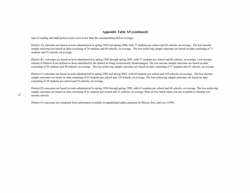
Appendix Table A5 (continued)
sum of reading and math pretest scores were lower than the corresponding district average.
District A's outcomes are based on tests administered in spring 1999 and spring 2000, with 77 students per school and 68 schools, on average. The low-income sample outcomes are based on data consisting of 76 students and 49 schools, on average. The low-achieving sample outcomes are based on data consisting of 71 students and 35 schools, on average.
District B's outcomes are based on tests administered in spring 1998 through spring 2003, with 57 students per school and 89 schools, on average. Low-income schools in District B are defined as those identified by the district as being economically disadvantaged. The low-income sample outcomes are based on data consisting of 58 students and 48 schools, on average. The low-achieving sample outcomes are based on data consisting of 57 students and 43 schools, on average.
District C's outcomes are based on tests administered in spring 2002 and spring 2003, with 69 students per school and 169 schools, on average. The low-income sample outcomes are based on data consisting of 62 students per school and 129 schools, on average. The low-achieving sample outcomes are based on data consisting of 59 students per school and 76 schools, on average.
District D's outcomes are based on tests administered in spring 1994 through spring 1999, with 65 students per school and 48 schools, on average. The low-achieving sample outcomes are based on data consisting of 61 students per school and 23 schools, on average. Data on free lunch status was not available to identify low-income schools.
District E's outcomes are computed from information available in unpublished tables prepared by Bloom, Bos, and Lee (1999).
71

72
Appendix Table A6
Grade 5 Reading
Minimum Detectable Effect Size (MDES) by Number of Randomized Schools (J) and Single Covariate
A B C E Mean
No covariate 0.68 0.53 0.61 0.40 0.56 Y-1 0.56 0.39 0.30 0.25 0.38 Y-2 0.56 0.43 0.34 0.28 0.40 Y-3 NA NA 0.36 NA (0.36) y-1 0.60 0.55 a 0.28 0.16 0.40 y-2 0.59 0.32 0.34 0.21 0.36 y-3 0.61 NA NA NA (0.61)
No covariate 0.47 0.37 0.42 0.29 0.38 Y-1 0.38 0.27 0.21 0.18 0.26 Y-2 0.38 0.30 0.24 0.20 0.28 Y-3 NA NA 0.25 NA (0.25) y-1 0.41 0.38 a 0.19 0.11 0.27 y-2 0.40 0.22 0.23 0.15 0.25 y-3 0.42 NA NA NA (0.42)
No covariate 0.38 0.30 0.34 0.23 0.31 Y-1 0.31 0.22 0.17 0.14 0.21 Y-2 0.31 0.24 0.19 0.16 0.22 Y-3 NA NA 0.20 NA (0.20) y-1 0.33 0.31 a 0.16 0.09 0.22 y-2 0.33 0.18 0.19 0.12 0.20 y-3 0.34 NA NA NA (0.34)
(continued)
MDES(J=40)
MDES(J=60)
Using Covariates to Improve Precision
CovariateFindings for District
MDES(J=20)
NOTES: In the last column, means in parenthesis indicate that the reported values do not include the values from all four districts. Y-1, Y-2, and Y-3 are mean school scores for the same grade lagged one, two, and three years, respectively. y-1, y-2, and y-3 are individual student scores lagged one, two, and three years, respectively. Findings reflect: statistical significance of 0.05, statistical power of 0.80, a two-tail hypothesis test, 60 students per school, and a balanced (50/50) allocation of schools to treatment and control status. Entries are computed using the mean of the corresponding district-level parameters. See Appendix Table A9 for these parameters.
District A's outcomes are based on tests administered in spring 1999 and spring 2000, with 66 students per school and 68 schools, on average. District B's outcomes are based on tests administered in spring 1997, with 48 students per school and 83 schools. District C's outcomes are based on tests administered in spring 2002 and

73
Appendix Table A6 (continued)
spring 2003, with 85 students per school and 171 schools, on average. District E's outcomes are for the sixth grade and are taken from Table 4 of Bloom, Bos, and Lee (1999).
aBeginning in 1996 a second test was also administered to 4th graders in District B. With the addition of this new test, the 4th grade scores for the former test fell. Thus, individual scores in the previous year for the 1997 cohort of 5th graders are not good predictors of their 5th grade test results. This is reflected in the table by the fact that the MDES for y-1 in District B is about as large as or larger than its MDES for no covariates.

74
Appendix Table A7
Grade 5 Reading
Minimum Detectable Effect Size for 40 Randomized Schools with Alternative Samples of Schools and Covariates
(Excluding District E)
A B C MeanAll schoolsNo covariate 0.47 0.37 0.42 0.42 Y-1 0.38 0.27 0.21 0.29 Y-1,Y-2 0.37 0.27 0.20 0.28 y-1 0.41 0.38 a 0.19 0.33 y-1,y-2 0.39 0.25 0.20 0.28 Y-1,y-1 0.38 0.33 0.18 0.30 Z-1 0.40 0.29 0.27 0.32 z-1 0.41 0.34 0.25 0.33 X 0.42 0.28 0.26 0.32 X,Y-1 0.37 0.23 0.19 0.26 X,y-1 0.40 0.33 0.19 0.31Low-income schools Y-1 0.41 0.25 0.22 0.29 y-1 0.43 0.27 a 0.24 0.31Low-achieving schools Y-1 0.41 0.24 0.23 0.30 y-1 0.44 0.35 a 0.25 0.35
(continued)
School sample and covariatesFindings for District
Using Covariates to Improve Precision
NOTES: Y-1 and Y-2 are mean school scores for the same grade lagged one and two years, respectively. y-1 and y-2 are individual student scores lagged one and two years, respectively. Z-1 and z-1 are mean school scores and individual scores in the previous year for a different test (with a math test as the pretest for reading outcomes and a reading test as the pretest for math outcomes). X is a vector of demographic characteristics, which differs across districts. Low-income schools are defined as those whose average proportion of students eligible for free lunch exceeds the district average. Low-achieving schools in the district are defined as those whose average combined sum of reading and math pretest scores were lower than the corresponding district average. Findings reflect: statistical significance of 0.05, statistical power of 0.80, a two-tail hypothesis test, 60 students per school, and a balanced (50/50) allocation of schools to treatment and control status.
District A's outcomes are based on tests administered in spring 1999 and spring 2000, with 66 students per school and 68 schools, on average. The low-income sample outcomes are based on data consisting of 63 students and 45 schools, on average. The low-achieving sample outcomes are based on data consisting of 63 students and 34 schools, on average.

75
Appendix Table A7 (continued)
District B's outcomes are based on tests administered in spring 1997, with 48 students per school and 83 schools. Low-income schools in District B are defined as those identified by the district as being economically disadvantaged. The low-income sample outcomes are based on data consisting of 47 students and 43 schools. The low-achieving sample outcomes are based on data consisting of 47 students and 41 schools.
District C's outcomes are based on tests administered in spring 2002 and spring 2003, with 85 students per school and 171 schools, on average. The low-income sample outcomes are based on data consisting of 78 students per school and 120 schools, on average. The low-achieving sample outcomes are based on data consisting of 75 students per school and 82 schools, on average.
aBeginning in 1996 a second test was also administered to 4th graders in District B. With the addition of this new test, the 4th grade scores for the former test fell. Thus, individual scores in the previous year for the 1997 cohort of 5th graders are not good predictors of their 5th grade test results. This is reflected in the table by the fact that the MDES for y-1 in District B is about as large as or larger than its MDES for no covariates.

76
Appendix Table A8
Grade 5 Reading
Minimum Detectable Effect Size Ranges for 40 Randomized Schools withAlternative Samples of Schools and Selected Covariates
(min, max) (min, max) (min, max) (min, max)All schools Y-1 (0.36, 0.41) (0.20, 0.21) (0.17, 0.18) y-1 (0.38, 0.45) (0.18, 0.20) (0.09, 0.13)Low-income schools Y-1 (0.38, 0.45) (0.22, 0.23) NA NA y-1 (0.38, 0.47) (0.22, 0.25) NA NALow-achieving schools Y-1 (0.35, 0.46) (0.23, 0.24) NA NA y-1 (0.37, 0.50) (0.24, 0.26) NA NA
Using Covariates to Improve Precision
(range not available)a
(range not available)a
(range not available)a
Findings for DistrictSchool sample and covariate A B C E
NOTES: Y-1 is the mean school score for the same grade lagged one year, and y-1 is the individual student score lagged one year. Low-income schools are defined as those whose average proportion of students eligible for free lunch exceeds the district average. Low-achieving schools in the district are defined as those whose average combined sum of reading and math pretest scores were lower than the corresponding district average. Findings reflect: statistical significance of 0.05, statistical power of 0.80, a two-tail hypothesis test, 60 students per school, and a balanced (50/50) allocation of schools to treatment and control status.
District A's outcomes are based on tests administered in spring 1999 and spring 2000, with 66 students per school and 68 schools, on average. The low-income sample outcomes are based on data consisting of 63 students and 45 schools, on average. The low-achieving sample outcomes are based on data consisting of 63 students and 34 schools, on average.
District C's outcomes are based on tests administered in spring 2002 and spring 2003, with 85 students per school and 171 schools, on average. The low-income sample outcomes are based on data consisting of 78 students per school and 120 schools, on average. The low-achieving sample outcomes are based on data consisting of 75 students per school and 82 schools, on average.
District E's outcomes are for the sixth grade and are taken from Table 4 of Bloom, Bos, and Lee (1999).
aThere is only one year of follow-up data for District B. Values for this year can be obtained from Appendix Table A7.

77
Appendix Table A9
Grade 5 Reading
Parameter Values for Selected Covariates
R2C R2
I R2C R2
I R2C R2
I R2C R2
I
Y-1 0.33 0.00 0.50 0.00 0.81 0.00 0.70 0.00Y-2 0.35 0.00 0.37 0.00 0.73 0.00 0.59 0.00Y-3 NA NA NA NA 0.70 0.00 NA NAY-1, Y-2 0.40 0.00 0.51 0.00 0.83 0.00 0.70 0.00Y-2, Y-3 NA NA NA NA 0.77 0.00 NA NA
y-1 0.21 0.29 -0.08 a 0.14 a 0.80 0.49 0.88 0.59y-2 0.25 0.24 0.67 0.36 0.71 0.37 0.74 0.42y-3 0.19 0.18 NA NA NA NA NA NAy-1, y-2 0.30 0.36 0.56 0.38 0.80 0.52 0.87 0.67y-2, y-3 0.26 0.29 NA NA NA NA NA NA
Y-1, y-1 0.35 0.29 0.20 0.14 0.83 0.49 NA NAZ-1 0.30 0.00 0.40 0.00 0.62 0.00 NA NAz-1 0.23 0.25 0.15 0.12 0.67 0.33 NA NAX 0.21 0.09 0.43 0.08 0.65 0.27 NA NAX, Y-1 0.40 0.09 0.64 0.08 0.84 0.27 NA NAX, y-1 0.26 0.32 0.18 0.19 0.81 0.53 NA NA
(continued)
0.12
Covariates Parameters for DistrictA B C E
Other covariates
Student-level pretests only
Using Covariates to Improve Precision
Proportion of variance reduced (R2C and R2
I)
School-level pretests only
Intra-class correlation with no covariates (ρ)0.25 0.15 0.20
NOTES: Y-1, Y-2, and Y-3 are mean school scores for the same grade lagged one, two, and three years, respectively. y-1, y-2, and y-3 are individual student scores lagged one, two, and three years, respectively. X is a vector of demographic characteristics, which differs across districts. Z-1 and z-1 are mean school scores and individual scores in the previous year for a different test (with a math test as the pretest for reading outcomes and a reading test as the pretest for math outcomes). R2
C and R2I are the average proportion of the school-level variance and the student-level
variance reduced by the covariates, respectively. The averages are computed as the mean of the corresponding district-level parameters. Nonzero estimates for R2
I with school level covariates only are set equal to zero. See text for more details.
District A's outcomes are based on tests administered in spring 1999 and spring 2000, with 66 students per school and 68 schools, on average. District B's outcomes are based on tests administered in spring 1997, with 48 students per school and 83 schools. District C's outcomes are based on tests administered in spring 2002 and spring 2003,

78
Appendix Table A9 (continued)
with 85 students per school and 171 schools, on average. District E's outcomes are for the sixth grade and were computed from information available in unpublished tables prepared by Bloom, Bos, and Lee (1999).
aBeginning in 1996 a second test was also administered to 4th graders in District B. With the addition of this new test, the 4th grade scores for the former test fell. Thus, individual scores in the previous year for the 1997 cohort of 5th graders are not good predictors of their 5th grade test results. This is reflected in the table by the fact that the average proportion of the school-level variance explained and the student-level variance explained by y-1 in District B is very small.
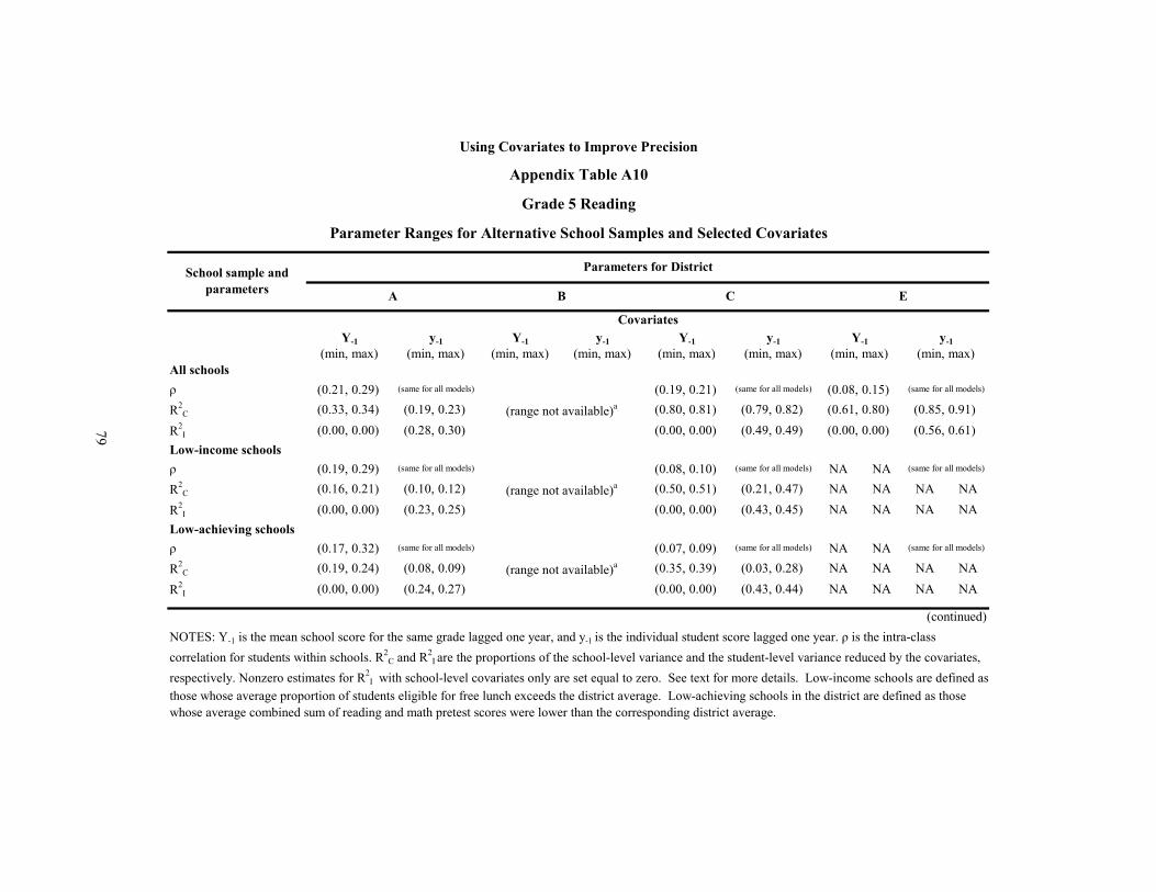
Appendix Table A10
Grade 5 Reading
Parameter Ranges for Alternative School Samples and Selected Covariates
(min, max) (min, max) (min, max) (min, max) (min, max) (min, max) (min, max) (min, max)All schoolsρ (0.21, 0.29) (0.19, 0.21) (0.08, 0.15)R2
C (0.33, 0.34) (0.19, 0.23) (0.80, 0.81) (0.79, 0.82) (0.61, 0.80) (0.85, 0.91)
R2I (0.00, 0.00) (0.28, 0.30) (0.00, 0.00) (0.49, 0.49) (0.00, 0.00) (0.56, 0.61)
ρ (0.19, 0.29) (0.08, 0.10) NA NAR2
C (0.16, 0.21) (0.10, 0.12) (0.50, 0.51) (0.21, 0.47) NA NA NA NA
R2I (0.00, 0.00) (0.23, 0.25) (0.00, 0.00) (0.43, 0.45) NA NA NA NA
ρ (0.17, 0.32) (0.07, 0.09) NA NAR2
C (0.19, 0.24) (0.08, 0.09) (0.35, 0.39) (0.03, 0.28) NA NA NA NA
R2I (0.00, 0.00) (0.24, 0.27) (0.00, 0.00) (0.43, 0.44) NA NA NA NA
(continued)
School sample and parameters
Parameters for District
A B C E
Covariatesy-1
(same for all models)
(range not available)a
(same for all models) (same for all models)
Y-1 y-1y-1 y-1Y-1
Using Covariates to Improve Precision
(same for all models)
Low-achieving schools
Low-income schools(same for all models)
(range not available)a
Y-1 Y-1
(same for all models)
(same for all models)
(range not available)a
(same for all models) (same for all models)
NOTES: Y-1 is the mean school score for the same grade lagged one year, and y-1 is the individual student score lagged one year. ρ is the intra-class correlation for students within schools. R2
C and R2I are the proportions of the school-level variance and the student-level variance reduced by the covariates,
respectively. Nonzero estimates for R2I with school-level covariates only are set equal to zero. See text for more details. Low-income schools are defined as
those whose average proportion of students eligible for free lunch exceeds the district average. Low-achieving schools in the district are defined as those whose average combined sum of reading and math pretest scores were lower than the corresponding district average.
79
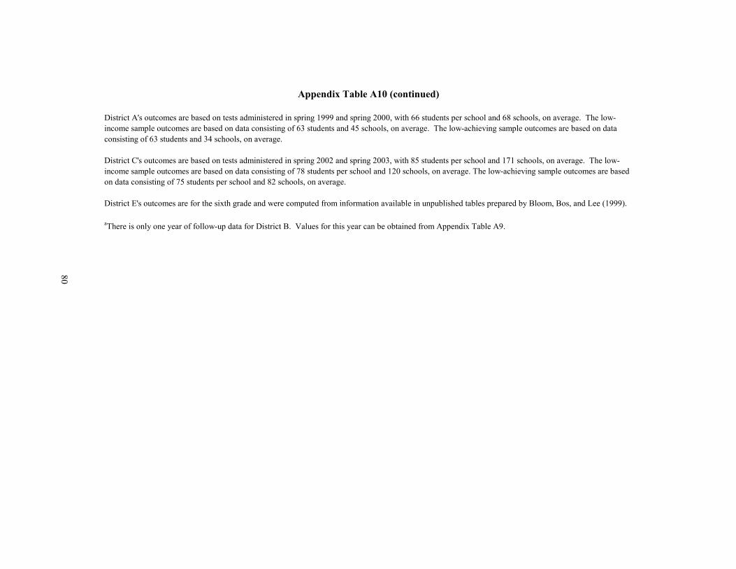
Appendix Table A10 (continued)
District A's outcomes are based on tests administered in spring 1999 and spring 2000, with 66 students per school and 68 schools, on average. The low-income sample outcomes are based on data consisting of 63 students and 45 schools, on average. The low-achieving sample outcomes are based on data consisting of 63 students and 34 schools, on average.
District C's outcomes are based on tests administered in spring 2002 and spring 2003, with 85 students per school and 171 schools, on average. The low-income sample outcomes are based on data consisting of 78 students per school and 120 schools, on average. The low-achieving sample outcomes are based on data consisting of 75 students per school and 82 schools, on average.
District E's outcomes are for the sixth grade and were computed from information available in unpublished tables prepared by Bloom, Bos, and Lee (1999).
aThere is only one year of follow-up data for District B. Values for this year can be obtained from Appendix Table A9.
80

81
Appendix Table A11
Grade 5 Math
Minimum Detectable Effect Size (MDES) by Number of Randomized Schools (J) and Single Covariate
A B C E Mean
No covariate 0.61 0.60 0.57 0.49 0.57 Y-1 0.45 0.42 0.35 0.28 0.38 Y-2 0.43 0.48 0.38 0.34 0.41 Y-3 0.48 NA 0.40 NA (0.44) y-1 0.43 0.56 a 0.32 0.25 0.39 y-2 0.44 0.38 0.38 0.34 0.38 y-3 0.50 NA NA NA (0.50)
No covariate 0.42 0.41 0.39 0.35 0.39 Y-1 0.31 0.29 0.24 0.20 0.26 Y-2 0.30 0.33 0.26 0.24 0.28 Y-3 0.33 NA 0.27 NA (0.30) y-1 0.30 0.38 a 0.22 0.18 0.27 y-2 0.30 0.26 0.26 0.24 0.27 y-3 0.34 NA NA NA (0.34)
No covariate 0.34 0.33 0.32 0.29 0.32 Y-1 0.25 0.23 0.20 0.16 0.21 Y-2 0.24 0.27 0.21 0.20 0.23 Y-3 0.27 NA 0.22 NA (0.24) y-1 0.24 0.31 a 0.18 0.15 0.22 y-2 0.24 0.21 0.21 0.20 0.22 y-3 0.28 NA NA NA (0.28)
(continued)
MDES(J=40)
MDES(J=60)
Using Covariates to Improve Precision
CovariateFindings for District
MDES(J=20)
NOTES: In the last column, means in parenthesis indicate that the reported values do not include the values from all four districts. Y-1, Y-2, and Y-3 are mean school scores for the same grade lagged one, two, and three years, respectively. y-1, y-2, and y-3 are individual student scores lagged one, two, and three years, respectively. Findings reflect: statistical significance of 0.05, statistical power of 0.80, a two-tail hypothesis test, 60 students per school, and a balanced (50/50) allocation of schools to treatment and control status. Entries are computed using the mean of the corresponding district-level parameters. See Appendix Table A14 for these parameters.
District A's outcomes are based on tests administered in spring 1999 and spring 2000, with 66 students per school and 68 schools, on average. District B's outcomes are based on tests administered in spring 1997, with 48 students per school and 83 schools. District C's outcomes are based on tests administered in spring 2002 and

82
Appendix Table A11 (continued)
spring 2003, with 85 students per school and 171 schools, on average. District E's outcomes are for the sixth grade and are taken from Table 4 of Bloom, Bos, and Lee (1999).
aBeginning in 1996 a second test was also administered to 4th graders in District B. With the addition of this new test, the 4th grade scores for the former test fell. Thus, individual scores in the previous year for the 1997 cohort of 5th graders are not good predictors of their 5th grade test results. This is reflected in the table by the fact that the MDES for y-1 in District B is about as large or larger than its MDES for no covariates.

83
Appendix Table A12
Grade 5 Math
Minimum Detectable Effect Size for 40 Randomized Schools withAlternative Samples of Schools and Covariates
(Excluding District E)
A B C MeanAll schoolsNo covariate 0.42 0.41 0.39 0.41 Y-1 0.31 0.29 0.24 0.28 Y-1,Y-2 0.28 0.29 0.23 0.26 y-1 0.30 0.38 a 0.22 0.30 y-1,y-2 0.27 0.27 0.22 0.26 Y-1,y-1 0.28 0.33 0.21 0.27 Z-1 0.31 0.29 0.24 0.28 z-1 0.30 0.38 0.22 0.30 X 0.32 0.34 0.27 0.31 X,Y-1 0.28 0.24 0.22 0.25 X,y-1 0.28 0.35 0.22 0.28Low-income schools Y-1 0.32 0.29 0.25 0.29 y-1 0.33 0.38 a 0.24 0.32Low-achieving schools Y-1 0.32 0.30 0.26 0.30 y-1 0.35 0.42 a 0.26 0.34
(continued)
School sample and covariatesFindings for District
Using Covariates to Improve Precision
NOTES: Y-1 and Y-2 are mean school scores for the same grade lagged one and two years, respectively. y-1 and y-2 are individual student scores lagged one and two years, respectively. Z-1 and z-1 are mean school scores and individual scores in the previous year for a different test (with a math test as the pretest for reading outcomes and a reading test as the pretest for math outcomes). X is a vector of demographic characteristics, which differs across districts. Low-income schools are defined as those whose average proportion of students eligible for free lunch exceeds the district average. Low-achieving schools in the district are defined as those whose average combined sum of reading and math pretest scores were lower than the corresponding district average. Findings reflect: statistical significance of 0.05, statistical power of 0.80, a two-tail hypothesis test,60 students per school, and a balanced (50/50) allocation of schools to treatment and control status.
District A's outcomes are based on tests administered in spring 1999 and spring 2000, with 66 students per school and 68 schools, on average. The low-income sample outcomes are based on data consisting of 63 students and 45 schools, on average. The low-achieving sample outcomes are based on data consisting of 63 students and 34 schools, on average.

84
Appendix Table A12 (continued)
District B's outcomes are based on tests administered in spring 1997, with 48 students per school and 83 schools. Low-income schools in District B are defined as those identified by the district as being economically disadvantaged. The low-income sample outcomes are based on data consisting of 47 students and 43 schools. The low-achieving sample outcomes are based on data consisting of 47 students and 41 schools.
District C's outcomes are based on tests administered in spring 2002 and spring 2003, with 85 students per school and 171 schools, on average. The low-income sample outcomes are based on data consisting of 78 students per school and 120 schools, on average. The low-achieving sample outcomes are based on data consisting of 75 students per school and 82 schools, on average.
aBeginning in 1996 a second test was also administered to 4th graders in District B. With the addition of this new test, the 4th grade scores for the former test fell. Thus, individual scores in the previous year for the 1997 cohort of 5th graders are not goods predictors of their 5th grade test results. This is reflected in the table by the fact that the MDES for y-1 in District B is about as large or larger than its MDES for no covariates.

85
Appendix Table A13
Grade 5 Math
Minimum Detectable Effect Size Ranges for 40 Randomized Schools withAlternative Samples of Schools and Selected Covariates
(min, max) (min, max) (min, max) (min, max)All schools Y-1 (0.30, 0.32) (0.23, 0.26) (0.18, 0.21) y-1 (0.27, 0.32) (0.22, 0.22) (0.16, 0.20)Low-income schools Y-1 (0.32, 0.33) (0.25, 0.25) NA NA y-1 (0.30, 0.36) (0.24, 0.25) NA NALow-achieving schools Y-1 (0.32, 0.33) (0.26, 0.27) NA NA y-1 (0.30, 0.38) (0.25, 0.26) NA NA
(range not available)a
(range not available)a
(range not available)a
School sample and covariate
Using Covariates to Improve Precision
Findings for DistrictA B C E
NOTES: Y-1 is the mean school score for the same grade lagged one year, and y-1 is the individual student score lagged one year. Low-income schools are defined as those whose average proportion of students eligible for free lunch exceeds the district average. Low-achieving schools in the district are defined as those whose average combined sum of reading and math pretest scores were lower than the corresponding district average. Findings reflect: statistical significance of 0.05, statistical power of 0.80, a two-tail hypothesis test, 60 students per school, and a balanced (50/50) allocation of schools to treatment and control status.
District A's outcomes are based on tests administered in spring 1999 and spring 2000, with 66 students per school and 68 schools, on average. The low-income sample outcomes are based on data consisting of 63 students and 45 schools, on average. The low-achieving sample outcomes are based on data consisting of 63 students and 34 schools, on average.
District C's outcomes are based on tests administered in spring 2002 and spring 2003, with 85 students per school and 171 schools, on average. The low-income sample outcomes are based on data consisting of 78 students per school and 120 schools, on average. The low-achieving sample outcomes are based on data consisting of 75 students per school and 82 schools, on average.
District E's outcomes are for the sixth grade and are taken from Table 4 of Bloom, Bos, and Lee (1999).
aThere is only one year of follow-up data for District B. Values for this year can be obtained from Appendix Table A12.

86
Appendix Table A14
Grade 5 Math
Parameter Values for Selected Covariates
R2C R2
I R2C R2
I R2C R2
I R2C R2
I
Y-1 0.47 0.00 0.54 0.00 0.66 0.00 0.73 0.00Y-2 0.53 0.00 0.39 0.00 0.60 0.00 0.59 0.00Y-3 0.41 0.00 NA NA 0.55 0.00 NA NAY-1, Y-2 0.60 0.00 0.55 0.00 0.72 0.00 0.76 0.00Y-2, Y-3 0.56 0.00 NA NA 0.64 0.00 NA NA
y-1 0.50 0.45 0.13 a 0.16 a 0.70 0.45 0.75 0.45y-2 0.49 0.33 0.62 0.37 0.57 0.32 0.55 0.35y-3 0.33 0.20 NA NA NA NA NA NAy-1, y-2 0.57 0.50 0.57 0.40 0.70 0.48 0.74 0.50y-2, y-3 0.52 0.37 NA NA NA NA NA NA
Y-1, y-1 0.57 0.45 0.37 0.16 0.73 0.45 NA NAZ-1 0.47 0.00 0.54 0.00 0.66 0.00 NA NAz-1 0.50 0.45 0.13 0.16 0.70 0.45 NA NAX 0.43 0.09 0.32 0.08 0.53 0.24 NA NAX, Y-1 0.60 0.09 0.69 0.08 0.70 0.24 NA NAX, y-1 0.56 0.47 0.30 0.21 0.70 0.50 NA NA
(continued)
0.17 0.18
Covariates Parameters for DistrictA C EB
Other covariates
Using Covariates to Improve Precision
Proportion of variance reduced (R2C and R2
I)
School-level pretests only
Student-level pretests only
Intra-class correlation with no covariates (ρ)0.20 0.19
NOTES: Y-1, Y-2, and Y-3 are mean school scores for the same grade lagged one, two, and three years, respectively. y-1, y-2, and y-3 are individual student scores lagged one, two, and three years, respectively. X is a vector of demographic characteristics, which differs across districts. Z-1 and z-1 are mean school scores and individual scores in the previous year for a different test (with a math test as the pretest for reading outcomes and a reading test as the pretest for math outcomes). R2
C and R2I are the average proportion of the school-level variance and the student-
level variance reduced by the covariates, respectively. The averages are computed as the mean of the corresponding district-level parameters. Nonzero estimates for R2
I with school level covariates only are set equal to zero. See text for more details.
District A's outcomes are based on tests administered in spring 1999 and spring 2000, with 66 students per school and 68 schools, on average. District B's outcomes are based on tests administered in spring 1997, with 48 students per school and 83 schools. District C's outcomes are based on tests administered in spring 2002 and spring 2003,

87
Appendix Table A14 (continued)
with 85 students per school and 171 schools, on average. District E's outcomes are for the sixth grade and were computed from information available in unpublished tables prepared by Bloom, Bos, and Lee (1999).
aBeginning in 1996 a second test was also administered to 4th graders in District B. With the addition of this new test, the 4th grade scores for the former test fell. Thus, individual scores in the previous year for the 1997 cohort of 5th graders are not good predictors of their 5th grade test results. This is reflected in the table by the fact that the average proportion of the school-level variance explained and the student-level variance explained by y-1 in District B is very small.
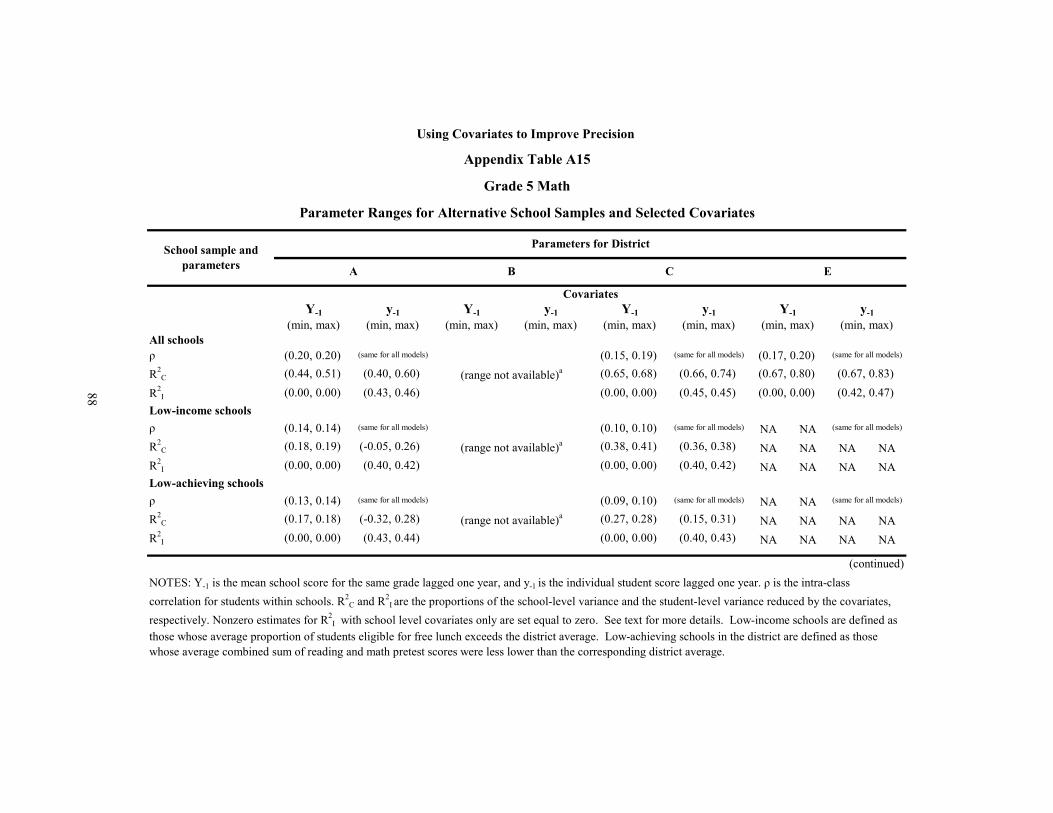
Appendix Table A15
Grade 5 Math
Parameter Ranges for Alternative School Samples and Selected Covariates
(min, max) (min, max) (min, max) (min, max) (min, max) (min, max) (min, max) (min, max)All schoolsρ (0.20, 0.20) (0.15, 0.19) (0.17, 0.20)R2
C (0.44, 0.51) (0.40, 0.60) (0.65, 0.68) (0.66, 0.74) (0.67, 0.80) (0.67, 0.83)
R2I (0.00, 0.00) (0.43, 0.46) (0.00, 0.00) (0.45, 0.45) (0.00, 0.00) (0.42, 0.47)
ρ (0.14, 0.14) (0.10, 0.10) NA NAR2
C (0.18, 0.19) (-0.05, 0.26) (0.38, 0.41) (0.36, 0.38) NA NA NA NAR2
I (0.00, 0.00) (0.40, 0.42) (0.00, 0.00) (0.40, 0.42) NA NA NA NA
ρ (0.13, 0.14) (0.09, 0.10) NA NAR2
C (0.17, 0.18) (-0.32, 0.28) (0.27, 0.28) (0.15, 0.31) NA NA NA NAR2
I (0.00, 0.00) (0.43, 0.44) (0.00, 0.00) (0.40, 0.43) NA NA NA NA
(continued)
School sample and parameters
Parameters for District
A B C E
CovariatesY-1 y-1 Y-1 y-1 Y-1 y-1 Y-1
(range not available)a
(same for all models)
y-1
(same for all models)
(range not available)a
(same for all models) (same for all models)
Using Covariates to Improve Precision
(same for all models)
Low-achieving schools(same for all models)
(range not available)a
(same for all models) (same for all models)
Low-income schools(same for all models)
NOTES: Y-1 is the mean school score for the same grade lagged one year, and y-1 is the individual student score lagged one year. ρ is the intra-class correlation for students within schools. R2
C and R2I are the proportions of the school-level variance and the student-level variance reduced by the covariates,
respectively. Nonzero estimates for R2I with school level covariates only are set equal to zero. See text for more details. Low-income schools are defined as
those whose average proportion of students eligible for free lunch exceeds the district average. Low-achieving schools in the district are defined as those whose average combined sum of reading and math pretest scores were less lower than the corresponding district average.
88

Appendix Table A15 (continued)
District A's outcomes are based on tests administered in spring 1999 and spring 2000, with 66 students per school and 68 schools, on average. Low-income schools in District B are defined as those identified by the district as being economically disadvantaged. The low-income sample outcomes are based on data consisting of 63 students and 45 schools, on average. The low-achieving sample outcomes are based on data consisting of 63 students and 34 schools, on average.
District C's outcomes are based on tests administered in spring 2002 and spring 2003, with 85 students per school and 171 schools, on average. The low-income sample outcomes are based on data consisting of 78 students per school and 120 schools, on average. The low-achieving sample outcomes are based on data consisting of 75 students per school and 82 schools, on average.
District E's outcomes are for the sixth grade and were computed from information available in unpublished tables prepared by Bloom, Bos, and Lee (1999).
aThere is only one year of follow-up data for District B. Values for this year can be obtained from Appendix Table A14.
89

90
Appendix Table A16
Grade 8 Reading
Minimum Detectable Effect Size (MDES) by Numberof Randomized Schools (J) and Single Covariate
A C Mean
No covariate 0.57 0.64 0.61 Y-1 0.28 0.21 0.24 Y-2 0.32 0.27 0.30 Y-3 NA 0.28 (0.28) y-1 0.38 0.18 0.28 y-2 0.31 0.24 0.27 y-3 NA 0.25 (0.25)
No covariate 0.39 0.44 0.42 Y-1 0.19 0.14 0.17 Y-2 0.22 0.18 0.20 Y-3 NA 0.19 (0.19) y-1 0.26 0.12 0.19 y-2 0.21 0.16 0.19 y-3 NA 0.17 (0.17)
No covariate 0.32 0.36 0.34 Y-1 0.16 0.11 0.13 Y-2 0.18 0.15 0.16 Y-3 NA 0.15 (0.15) y-1 0.21 0.10 0.15 y-2 0.17 0.13 0.15 y-3 NA 0.14 (0.14)
MDES(J=40)
MDES(J=60)
Using Covariates to Improve Precision
CovariateFindings for District
MDES(J=20)
NOTES: In the last column, means in parenthesis indicate that the reported values donot include the values from both districts. Y-1, Y-2, and Y-3 are mean school scores fothe same grade lagged one, two, and three years, respectively. y-1, y-2, and y-3 are individual student scores lagged one, two, and three years, respectively. Findings reflect: statistical significance of 0.05, statistical power of 0.80, a two-tail hypothesis test, 250 students per school, and a balanced (50/50) allocation of schools to treatmenand control status. Entries are computed using the mean of the corresponding district-level parameters. See Appendix Table A19 for these parameters.
District A's outcomes are based on tests administered in spring 1999 and spring 2000with 202 students per school and 17 schools, on average. District C's outcomes are based on tests administered in spring 2002 and spring 2003, with 297 students per school and 41 schools, on average.

91
Appendix Table A17
Grade 8 Reading
Minimum Detectable Effect Size for 40 Randomized Schools with Alternative Samples of Schools and Covariates
A C MeanAll schoolsNo covariate 0.39 0.44 0.42 Y-1 0.19 0.14 0.17 Y-1,Y-2 0.19 0.14 0.16 y-1 0.26 0.12 0.19 y-1,y-2 0.21 0.12 0.16 Y-1,y-1 0.20 0.11 0.16 Z-1 0.20 0.20 0.20 z-1 0.27 0.19 0.23 X 0.30 0.30 0.30 X,Y-1 0.17 0.16 0.17 X,y-1 0.23 0.12 0.18Low-income schools Y-1 0.17 0.17 0.17 y-1 0.26 0.14 0.20Low-achieving schools Y-1 0.24 0.08 0.16 y-1 0.25 0.07 0.16
School sample and covariatesFindings for District
Using Covariates to Improve Precision
NOTES: Y-1 and Y-2 are mean school scores for the same grade lagged one and two years, respectively. y-1 and y-2 are individual student scores lagged one and two years, respectively. Z-1 and z-1 are mean school scores and individual scores in the previous year for a different test (with a math test as the pretest for reading outcomes and a reading test as the pretest for math outcomes). X is a vector of demographic characteristics, which differs across districts. Low-income schools are definedas those whose average proportion of students eligible for free lunch exceeds the district average. Low-achieving schools in the district are defined as those whose average combined sum of reading and math pretest scores were lower than the corresponding district average. Findings reflect: statistical significance of 0.05, statistical power of 0.80, a two-tail hypothesis test, 250 students per school, and a balanced (50/50) allocation of schools to treatment and control status.
District A's outcomes are based on tests administered in spring 1999 and spring 2000, with 202 students per school and 17 schools, on average. The low-income sample outcomes are based on data consisting of 183 students and 11 schools, on average. The low-achieving sample outcomes are based on data consisting of 158 students and 10 schools, on average.
District C's outcomes are based on tests administered in spring 2002 and spring 2003, with 297 students per school and 41 schools, on average. The low-income sample outcomes are based on data consisting of 292 students per school and 29 schools, on average. The low-achieving sample outcomes are based on data consisting of 262 students per school and 16 schools, on average.

92
Appendix Table A18
Grade 8 Reading
Minimum Detectable Effect Size (MDES) by Number ofRandomized Schools with Alternative Samples of
Schools and Selected Covariates
(min, max) (min, max)All schools Y-1 (0.18, 0.20) (0.09, 0.18) y-1 (0.22, 0.30) (0.10, 0.14)Low-income schools Y-1 (0.14, 0.20) (0.09, 0.22) y-1 (0.21, 0.30) (0.11, 0.17)Low-achieving schools Y-1 (0.21, 0.25) (0.08, 0.09) y-1 (0.16, 0.34) (0.05, 0.08)
Using Covariates to Improve Precision
Findings for DistrictSchool sample and covariate A C
NOTES: Y-1 is the mean school score for the same grade lagged one year, and y-1
is the individual student score lagged one year. Low-income schools are defined as those whose average proportion of students eligible for free lunch exceeds the district average. Low-achieving schools in the district are defined as those whose average combined sum of reading and math pretest scores were lower than the corresponding district average. Findings reflect: statistical significance of 0.05, statistical power of 0.80, a two-tail hypothesis test, 250 students per school, and a balanced (50/50) allocation of schools to treatment and control status.
District A's outcomes are based on tests administered in spring 1999 and spring 2000, with 202 students per school and 17 schools, on average. The low-income sample outcomes are based on data consisting of 183 students and 11 schools, on average. The low-achieving sample outcomes are based on data consisting of 158 students and 10 schools, on average.
District C's outcomes are based on tests administered in spring 2002 and spring 2003, with 297 students per school and 41 schools, on average. The low-income sample outcomes are based on data consisting of 292 students per school and 29 schools, on average. The low-achieving sample outcomes are based on data consisting of 262 students per school and 16 schools, on average.

93
Appendix Table A19
Grade 8 Reading
Minimum Detectable Effect Size (MDES) by Number
R2C R2
I R2C R2
I
Y-1 0.77 0.00 0.91 0.00Y-2 0.69 0.00 0.84 0.00Y-3 NA NA 0.83 0.00Y-1, Y-2 0.79 0.00 0.91 0.00Y-2, Y-3 NA NA 0.84 0.00
y-1 0.57 0.41 0.93 0.58y-2 0.72 0.41 0.87 0.49y-3 NA NA 0.85 0.42y-1, y-2 0.73 0.50 0.93 0.62y-2, y-3 NA NA 0.89 0.53
Y-1, y-1 0.75 0.41 0.94 0.58Z-1 0.75 0.00 0.81 0.00z-1 0.54 0.33 0.82 0.38X 0.43 0.11 0.55 0.23X, Y-1 0.83 0.11 0.87 0.23X, y-1 0.65 0.43 0.93 0.60
0.23
CovariatesA C
Other covariates
Using Covariates to Improve Precision
Findings for District
Proportion of variance reduced (R2C and R2
I)
Intra-class correlation with no covariates (ρ)
School-level pretests only
Student-level pretests only
0.18
NOTES: Y-1, Y-2, and Y-3 are mean school scores for the same grade lagged one, two, and three years, respectively. y-1, y-2, and y-3 are individual student scores lagged one, two, and three years, respectively. X is a vector of demographic characteristics, which differs across districts. Z-1 and z-1 are mean school scores and individual scores in the previous year for a different test (with a math test as the pretest for reading outcomes and a reading test as the pretest for math outcomes). R2
C and R2I are the average proportion of the school-level
variance and the student-level variance reduced by the covariates, respectively. The averages are computed as the mean of the corresponding district-level parameters. Nonzero estimates for R2
I with school-level covariates only are set equal to zero. See text for more details.
District A's outcomes are based on tests administered in spring 1999 and spring 2000, with 202 students per school and 17 schools, on average. District C's outcomes are based on tests administered in spring 2002 and spring 2003, with 297 students per school and 41 schools, on average.
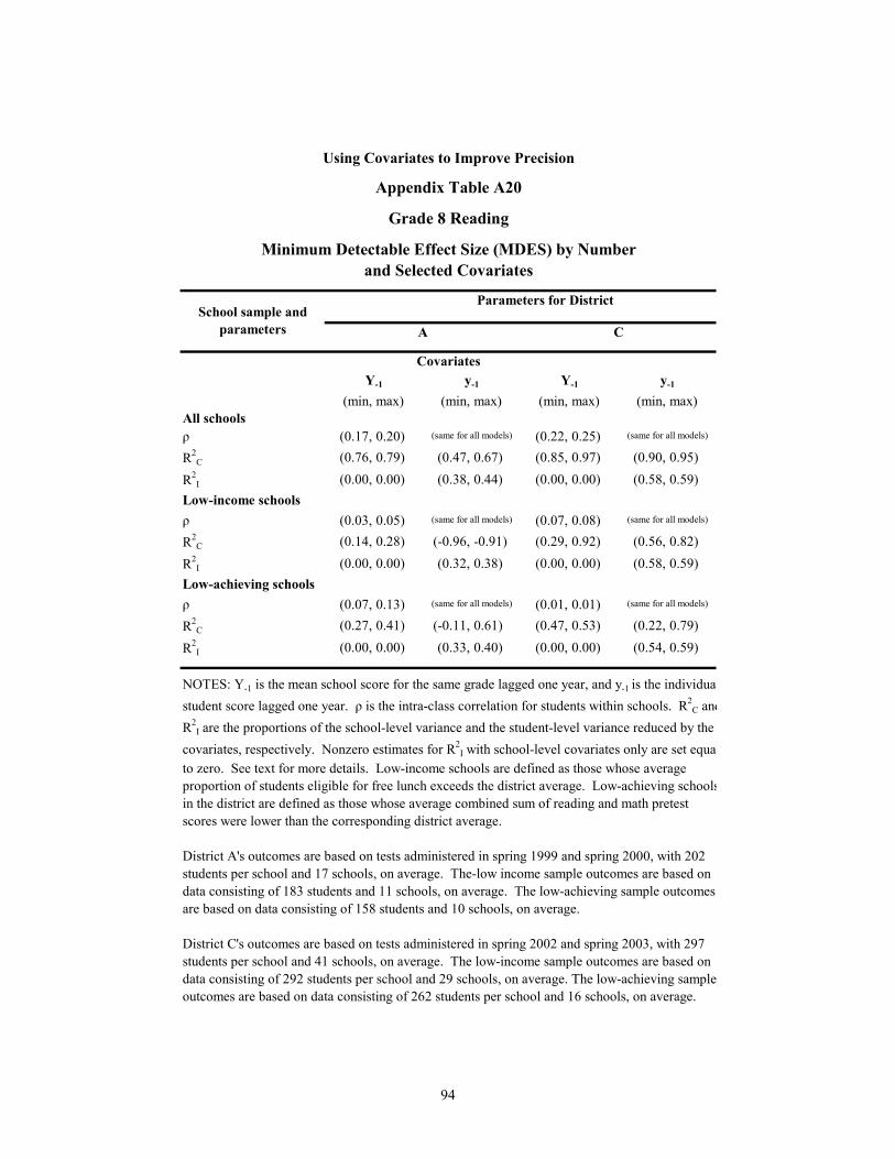
94
Appendix Table A20
Grade 8 Reading
Minimum Detectable Effect Size (MDES) by Numberand Selected Covariates
(min, max) (min, max) (min, max) (min, max)All schoolsρ (0.17, 0.20) (0.22, 0.25)R2
C (0.76, 0.79) (0.47, 0.67) (0.85, 0.97) (0.90, 0.95)
R2I (0.00, 0.00) (0.38, 0.44) (0.00, 0.00) (0.58, 0.59)
ρ (0.03, 0.05) (0.07, 0.08)R2
C (0.14, 0.28) (-0.96, -0.91) (0.29, 0.92) (0.56, 0.82)
R2I (0.00, 0.00) (0.32, 0.38) (0.00, 0.00) (0.58, 0.59)
ρ (0.07, 0.13) (0.01, 0.01)R2
C (0.27, 0.41) (-0.11, 0.61) (0.47, 0.53) (0.22, 0.79)
R2I (0.00, 0.00) (0.33, 0.40) (0.00, 0.00) (0.54, 0.59)
Y-1 y-1
Low-achieving schools
(same for all models) (same for all models)
Low-income schools
Y-1 y-1
(same for all models) (same for all models)
(same for all models) (same for all models)
Using Covariates to Improve Precision
Parameters for District
Covariates
School sample and parameters A C
NOTES: Y-1 is the mean school score for the same grade lagged one year, and y-1 is the individualstudent score lagged one year. ρ is the intra-class correlation for students within schools. R2
C andR2
I are the proportions of the school-level variance and the student-level variance reduced by the covariates, respectively. Nonzero estimates for R2
I with school-level covariates only are set equalto zero. See text for more details. Low-income schools are defined as those whose average proportion of students eligible for free lunch exceeds the district average. Low-achieving schoolsin the district are defined as those whose average combined sum of reading and math pretest scores were lower than the corresponding district average.
District A's outcomes are based on tests administered in spring 1999 and spring 2000, with 202 students per school and 17 schools, on average. The-low income sample outcomes are based on data consisting of 183 students and 11 schools, on average. The low-achieving sample outcomes are based on data consisting of 158 students and 10 schools, on average.
District C's outcomes are based on tests administered in spring 2002 and spring 2003, with 297 students per school and 41 schools, on average. The low-income sample outcomes are based on data consisting of 292 students per school and 29 schools, on average. The low-achieving sample outcomes are based on data consisting of 262 students per school and 16 schools, on average.

95
Appendix Table A21
Grade 8 Math
Minimum Detectable Effect Size (MDES) by Numberof Randomized Schools (J) and Single Covariate
A C Mean
No covariate 0.53 0.69 0.61 Y-1 0.26 0.29 0.28 Y-2 0.34 0.37 0.35 Y-3 0.36 0.37 0.37 y-1 0.28 0.29 0.28 y-2 0.29 0.36 0.33 y-3 0.31 0.40 0.36
No covariate 0.36 0.47 0.42 Y-1 0.18 0.20 0.19 Y-2 0.23 0.25 0.24 Y-3 0.25 0.26 0.25 y-1 0.19 0.20 0.19 y-2 0.20 0.25 0.22 y-3 0.21 0.28 0.24
No covariate 0.29 0.38 0.34 Y-1 0.14 0.16 0.15 Y-2 0.19 0.20 0.20 Y-3 0.20 0.21 0.20 y-1 0.15 0.16 0.16 y-2 0.16 0.20 0.18 y-3 0.17 0.22 0.20
MDES(J=40)
MDES(J=60)
Using Covariates to Improve Precision
CovariateFindings for District
MDES(J=20)
NOTES: Y-1, Y-2, and Y-3 are mean school scores for the same grade lagged one, two, and three years, respectively. y-1, y-2, and y-3 are individual student scores lagged one, two, and three years, respectively. Findings reflect: statistical significance of 0.05, statistical power of 0.80, a two-tail hypothesis test, 250 students per school, and a balanced (50/50) allocation of schools to treatment and control status. Entries are computed using the mean of the corresponding district-level parameters. See Appendix Table A24 for these parameters.
District A's outcomes are based on tests administered in spring 1999 and spring 2000, with 202 students per school and 17 schools, on average. District C's outcomes are based on tests administered in spring 2002 and spring 2003, with 297 students per school and 41 schools, on average.

96
Appendix Table A22
Grade 8 Math
Minimum Detectable Effect Size for 40 Randomized Schools with Alternative Samples of Schools and Covariates
A C MeanAll schoolsNo covariate 0.36 0.47 0.42 Y-1 0.18 0.20 0.19 Y-1,Y-2 0.18 0.20 0.19 y-1 0.19 0.20 0.19 y-1,y-2 0.17 0.20 0.19 Y-1,y-1 0.16 0.18 0.17 Z-1 0.18 0.20 0.19 z-1 0.19 0.20 0.19 X 0.27 0.34 0.31 X,Y-1 0.17 0.22 0.19 X,y-1 0.17 0.20 0.19Low-income schools Y-1 0.19 0.24 0.21 y-1 0.21 0.24 0.23Low-achieving schools Y-1 0.20 0.17 0.18 y-1 0.21 0.13 0.17
School sample and covariatesFindings for District
Using Covariates to Improve Precision
NOTES: Y-1 and Y-2 are mean school scores for the same grade lagged one and two years, respectively. y-1 and y-2 are individual student scores lagged one and two years, respectively. Z-1
and z-1 are mean school scores and individual scores in the previous year for a different test (with a math test as the pretest for reading outcomes and a reading test as the pretest for math outcomes). X is a vector of demographic characteristics, which differs across districts. Low-income schools are defined as those whose average proportion of students eligible for free lunch exceeds the district average. Low-achieving schools in the district are defined as those whose average combined sum of reading and math pretest scores were lower than the corresponding district average. Findings reflect: statistical significance of 0.05, statistical power of 0.80, a two-tail hypothesis test, 250 students per school, and a balanced (50/50) allocation of schools to treatment and control status.
District A's outcomes are based on tests administered in spring 1999 and spring 2000, with 202 students per school and 17 schools, on average. The low-income sample outcomes are based on data consisting of 183 students and 11 schools, on average. The low-achieving sample outcomes are based on data consisting of 158 students and 10 schools, on average.
District C's outcomes are based on tests administered in spring 2002 and spring 2003, with 297 students per school and 41 schools, on average. The low-income sample outcomes are based on data consisting of 292 students per school and 29 schools, on average. The low-achieving sample outcomes are based on data consisting of 262 students per school and 16 schools, on average.

97
Appendix Table A23
Grade 8 Math
Minimum Detectable Effect Size Ranges for 40 Randomized Schools with Alternative
Samples of Schools and Selected Covariates
(min, max) (min, max)All schools Y-1 (0.17, 0.18) (0.13, 0.26) y-1 (0.15, 0.22) (0.17, 0.23)Low-income schools Y-1 (0.17, 0.21) (0.14, 0.32) y-1 (0.16, 0.26) (0.18, 0.29)Low-achieving schools Y-1 (0.20, 0.20) (0.16, 0.17) y-1 (0.15, 0.28) (0.11, 0.14)
Using Covariates to Improve Precision
School sample and covariate A CFindings for District
NOTES: Y-1 is the mean school score for the same grade lagged one year, and y-1 is the individual student score lagged one year. Low-income schools are defined as those whose average proportion of students eligible for free lunch exceeds the district average. Low-achieving schools in the district are defined as those whose average combined sum of reading and math pretest scores were lower than the corresponding district average. Findings reflect: statistical significance of 0.05, statistical power of 0.80, a two-tail hypothesis test, 250 students per school, and a balanced (50/50) allocation of schools to treatment and control status.
District A's outcomes are based on tests administered in spring 1999 and spring 2000, with 202 students per school and 17 schools, on average. The low-income sample outcomes are based on data consisting of 183 students and 11 schools, on average. The low-achieving sample outcomes are based on data consisting of 158 students and 10 schools, on average.
District C's outcomes are based on tests administered in spring 2002 and spring 2003, with 297 students per school and 41 schools, on average. The low-income sample outcomes are based on data consisting of 292 students per school and 29 schools, on average. The low-achieving sample outcomes are based on data consisting of 262 students per school and 16 schools, on average.

98
Appendix Table A24
Grade 8 Math
Parameter Values for Selected Covariates
R2C R2
I R2C R2
I
Y-1 0.78 0.00 0.83 0.00Y-2 0.60 0.00 0.73 0.00Y-3 0.54 0.00 0.72 0.00Y-1, Y-2 0.78 0.00 0.83 0.00Y-2, Y-3 0.71 0.00 0.73 0.00
y-1 0.73 0.55 0.83 0.55y-2 0.70 0.49 0.73 0.48y-3 0.67 0.37 0.66 0.38y-1, y-2 0.78 0.61 0.82 0.59y-2, y-3 0.77 0.53 0.74 0.50
Y-1, y-1 0.82 0.55 0.86 0.55Z-1 0.78 0.00 0.83 0.00z-1 0.73 0.55 0.83 0.55X 0.45 0.10 0.48 0.20X, Y-1 0.80 0.10 0.79 0.20X, y-1 0.77 0.56 0.83 0.57
Other covariate models
Parameters for District
Intra-class correlation with no covariates (ρ)
Proportion of variance reduced (R2C and R2
I)
School-level pretests only
Student-level pretests only
Using Covariates to Improve Precision
0.16 0.27
CovariatesA C
NOTES: Y-1, Y-2, and Y-3 are mean school scores for the same grade lagged one, two, and three years, respectively. y-1, y-2, and y-3 are individual student scores lagged one, two, and three years, respectively. X is a vector of demographic characteristics, which differs across districts. Z-1 and z-1 are mean school scores and individual scores in the previous year for a different test (with a math test as the pretest for reading outcomes and a reading test as the pretest for math outcomes). R2
C and R2I are the average proportion of the school-level variance and the student-
level variance reduced by the covariates, respectively. The averages are computed as the mean of the corresponding district-level parameters. Nonzero estimaties for R2
I with school-level covariates only are set equal to zero. See text for more details.
District A's outcomes are based on tests administered in spring 1999 and spring 2000, with 202 students per school and 17 schools, on average. District C's outcomes are based on tests administered in spring 2002 and spring 2003, with 297 students per school and 41 schools, on average.

99
Appendix Table A25
Grade 8 Math
Parameter Ranges for Alternative School Samplesand Selected Covariates
(min, max) (min, max) (min, max) (min, max)All schoolsρ (0.15, 0.16) (0.25, 0.28)R2
C (0.78, 0.78) (0.63, 0.83) (0.72, 0.93) (0.78, 0.87)
R2I (-0.00, 0.00) (0.54, 0.56) (-0.00, 0.00) (0.54, 0.56)
ρ (0.06, 0.06) (0.10, 0.12)R2
C (0.23, 0.48) (-0.30, 0.50) (-0.01, 0.81) (0.19, 0.62)
R2I (-0.00, 0.00) (0.48, 0.51) (-0.00, 0.00) (0.50, 0.53)
ρ (0.06, 0.10) (0.04, 0.05)R2
C (0.31, 0.54) (0.05, 0.62) (0.13, 0.43) (0.38, 0.72)
R2I (0.00, 0.00) (0.51, 0.52) (-0.00, 0.00) (0.49, 0.54)
Low-income schools(same for all models) (same for all models)
(same for all models)
School sample and parameters A C
Y-1
(same for all models) (same for all models)
Using Covariates to Improve Precision
Parameters for District
Covariatesy-1 Y-1 y-1
Low-achieving schools
(same for all models)
NOTES: Y-1 is the mean school score for the same grade lagged one year, and y-1 is the individual student score lagged one year. ρ is the intra-class correlation for students within schools. R2
C and R2
I are the proportions of the school-level variance and the student-level variance reduced by the covariates, respectively. Nonzero estimates for R2
I with school-level covariates only are set to zero. See text for more details. Low-income schools are defined as those whose average proportion of students eligible for free lunch exceeds the district average. Low-achieving schools in the district are defined as those whose average combined sum of reading and math pre-test scores were lower than the corresponding district average.
District A's outcomes are based on tests administered in spring 1999 and spring 2000, with 202 students per school and 17 schools, on average. The low-income sample outcomes are based on data consisting of 183 students and 11 schools, on average. The low-achieving sample outcomes are based on data consisting of 158 students and 10 schools, on average.
District C's outcomes are based on tests administered in spring 2002 and spring 2003, with 297 students per school and 41 schools, on average. The low-income sample outcomes are based on data consisting of 292 students per school and 29 schools, on average. The low-achieving sample outcomes are based on data consisting of 262 students per school and 16 schools, on average.

100
Grade 10 Reading
Minimum Detectable Effect Size (MDES) by Numberof Randomized Schools (J) and Single Covariate
A C Mean
No covariate 0.53 0.71 0.62 Y-1 0.16 0.17 0.16 Y-2 0.23 0.24 0.24 Y-3 NA 0.26 (0.26) y-1 0.11 0.19 0.15 y-2 NA 0.25 (0.25) y-3 NA 0.25 (0.25)
No covariate 0.36 0.49 0.42 Y-1 0.11 0.12 0.11 Y-2 0.16 0.16 0.16 Y-3 NA 0.18 (0.18) y-1 0.08 0.13 0.10 y-2 NA 0.17 (0.17) y-3 NA 0.17 (0.17)
No covariate 0.29 0.39 0.34 Y-1 0.09 0.10 0.09 Y-2 0.13 0.13 0.13 Y-3 NA 0.14 (0.14) y-1 0.06 0.11 0.08 y-2 NA 0.14 (0.14) y-3 NA 0.14 (0.14)
MDES(J=40)
MDES(J=60)
Using Covariates to Improve Precision
Appendix Table A26
CovariateFindings for District
MDES(J=20)
NOTES: In the last column, means in parenthesis indicate that the reported values donot include the values from both districts. Y-1, Y-2, and Y-3 are mean school scores fothe same grade lagged one, two, and three years, respectively. y-1, y-2, and y-3 are individual student scores lagged one, two, and three years, respectively. Findings reflect: statistical significance of 0.05, statistical power of 0.80, a two-tail hypothesistest, 250 students per school, and a balanced (50/50) allocation of schools to treatmenand control status. Entries are computed using the mean of the corresponding districtlevel parameters. See Appendix Table A29 for these parameters.
District A's outcomes are based on tests administered in spring 1997 and spring 1998with 229 students per school and 12 schools, on average. District C's outcomes are based on tests administered in spring 2002 and spring 2003, with 265 students per school and 32 schools, on average.

101
Appendix Table A27
Grade 10 Reading
Minimum Detectable Effect Size for 40 Randomized Schools with Alternative Samples of Schools and Covariates
A C MeanAll schoolsNo covariate 0.36 0.49 0.42 Y-1 0.11 0.12 0.11 Y-1,Y-2 0.11 0.11 0.11 y-1 0.08 0.13 0.10 y-1,y-2 NA 0.11 (0.11) Y-1,y-1 0.05 0.08 0.07 Z-1 0.15 0.20 0.18 z-1 0.18 0.23 0.21 X 0.22 0.32 0.27 X,Y-1 0.07 0.14 0.11 X,y-1 0.07 0.11 0.09Low-income schools Y-1 NA 0.14 (0.14) y-1 NA 0.12 (0.12)Low-achieving schools Y-1 NA 0.13 (0.13) y-1 NA 0.11 (0.11)
Using Covariates to Improve Precision
School sample and covariates
Findings for District
NOTES: In the last column, means in parenthesis indicate that the reported values do not include the values from both districts. Y-1 and Y-2 are mean school scores for the same grade lagged one and two years, respectively. y-1 and y-2 are individual student scores lagged one and two years, respectively. Z-1 and z-1 are mean school scores and individual scores in the previous year for a different test (with a math test as the pretest for reading outcomes and a reading test as the pretest for math outcomes). X is a vector of demographic characteristics, which differs across districts. Low-income schools are defined as those whose average proportion of students eligible for free lunch exceeds the district average. Low-achieving schools in the district are defined as those whose average combined sum of reading and math pretest scores were lower than the corresponding district average. Findings reflect: statistical significance of 0.05, statistical power of 0.80, a two-tail hypothesis test, 250 students per school, and a balanced (50/50) allocation of schools to treatment and control status.
District A's outcomes are based on tests administered in spring 1997 and spring 1998, with 229 students per school and 12 schools, on average. Outcomes for low-income and low-achieving schools are not presented due to the small number of schools available.
District C's outcomes are based on tests administered in spring 2002 and spring 2003, with 265 students per school and 32 schools, on average. The low-income sample outcomes are based on data consisting of 237 students per school and 20 schools, on average. The low-achieving sample outcomes are based on data consisting of 204 students per school and 11 schools, on average.

102
Appendix Table A28
Grade 10 Reading
Minimum Detectable Effect Size Ranges for 40 Randomized Schools with Alternative Samples
of Schools and Selected Covariates
(min, max) (min, max)All schools Y-1 (0.10, 0.11) (0.10, 0.13) y-1 (0.06, 0.09) (0.13, 0.14)Low-income schools Y-1 NA NA (0.13, 0.15) y-1 NA NA (0.12, 0.12)Low-achieving schools Y-1 NA NA (0.11, 0.13) y-1 NA NA (0.10, 0.11)
Using Covariates to Improve Precision
Findings for DistrictSchool sample and covariate A C
NOTES: Y-1 is the mean school score for the same grade lagged one year, and y-1 is the individual student score lagged one year. Low-income schools are defined as those whose average proportion of students eligible for free lunch exceeds the district average. Low-achieving schools in the district are defined as those whose average combined sum of reading and math pretest scores were lower than the corresponding district average. Findings reflect: statistical significance of 0.05, statistical power of 0.80, a two-tail hypothesis test, 250 students per school, and a balanced (50/50) allocation of schools to treatment and control status.
District A's outcomes are based on tests administered in spring 1997 and spring 1998, with 229 students per school and 12 schools, on average. Outcomes for low-income and low-achieving schools are not presented due to the small number of schools available.
District C's outcomes are based on tests administered in spring 2002 and spring 2003, with 265 students per school and 32 schools, on average. The low-income sample outcomes are based on data consisting of 237 students per school and 20 schools, on average. The low-achieving sample outcomes are based on data consisting of 204 students per school and 11 schools, on average.

103
Appendix Table A29
Grade 10 Reading
Parameter Values for Selected Covariates
R2C R2
I R2C R2
I
Y-1 0.93 0.00 0.95 0.00Y-2 0.82 0.00 0.90 0.00Y-3 NA NA 0.88 0.00Y-1, Y-2 0.93 0.00 0.96 0.00Y-2, Y-3 NA NA 0.91 0.00
y-1 0.96 0.56 0.93 0.56y-2 NA NA 0.88 0.45y-3 NA NA 0.88 0.42y-1, y-2 NA NA 0.96 0.60y-2, y-3 NA NA 0.92 0.49
Y-1, y-1 0.99 0.56 0.98 0.56Z-1 0.83 0.00 0.84 0.00z-1 0.76 0.33 0.77 0.33X 0.63 0.18 0.59 0.19X, Y-1 0.97 0.18 0.92 0.19X, y-1 0.97 0.57 0.95 0.58
Using Covariates to Improve Precision
0.15 0.29
CovariatesA C
Other covariates
Proportion of variance reduced (R2C and R2
I)
Intra-class correlation with no covariates (ρ)
Parameters for District
School-level pretests only
Student-level pretests only
NOTES: Y-1, Y-2, and Y-3 are mean school scores for the same grade lagged one, two, and three years, respectively. y-1, y-2, and y-3 are individual student scores lagged one, two, and three years, respectively. X is a vector of demographic characteristics, which differs across districts. Z-1 and z-1 are mean school scores and individual scores in the previous year for a different test (with a math test as the pretest for reading outcomes and a reading test as the pretest for math outcomes). R2
C and R2I are the average
proportion of the school-level variance and the student-level variance reduced by the covariates, respectively. The averages are computed as the mean of the corresponding district-level parameters. Nonzero estimates for R2
I with school-level covariates only are set equal to zero. See text for more details.
District A's outcomes are based on tests administered in spring 1997 and spring 1998, with 229 students per school and 12 schools, on average. District C's outcomes are based on tests administered in spring 2002 and spring 2003, with 265 students per school and 32 schools, on average.

104
Appendix Table A30
Grade 10 Reading
Parameter Ranges for Alternative School Samplesand Selected Covariates
(min, max) (min, max) (min, max) (min, max)All schoolsρ (0.14, 0.17) (0.27, 0.30)R2
C (0.93, 0.94) (0.94, 0.98) (0.94, 0.96) (0.93, 0.93)
R2I (0.00, 0.00) (0.54, 0.57) (0.00, 0.00) (0.55, 0.57)
ρ NA NA (0.13, 0.15)R2
C NA NA NA NA (0.83, 0.87) (0.87, 0.91)
R2I NA NA NA NA (0.00, 0.00) (0.50, 0.54)
ρ NA NA (0.02, 0.03)R2
C NA NA NA NA (-0.14, 0.56) (0.17, 0.63)
R2I NA NA NA NA (0.00, 0.00) (0.47, 0.47)
Low-achieving schools(same for all models) (same for all models)
Low-income schools(same for all models) (same for all models)
Covariates
(same for all models) (same for all models)
Y-1 y-1 Y-1 y-1
Using Covariates to Improve Precision
School sample and parameters A C
Parameters for District
NOTES: Y-1 is the mean school score for the same grade lagged one year, and y-1 is the individual student score lagged one year. ρ is the intra-class correlation for students within schools. R2
C and R2I are the proportions of the school-level variance and the student-level
variance reduced by the covariates, respectively. Nonzero estimates for R2I with school-level
covariates only are set equal to zero. See text for more details. Low-income schools are defined as those whose average proportion of students eligible for free lunch exceeds the district average. Low-achieving schools in the district are defined as those whose average combined sum of reading and math pretest scores were lower than the corresponding district average.
District A's outcomes are based on tests administered in spring 1997 and spring 1998, with 229 students per school and 12 schools, on average. Outcomes for low-income and low-achieving schools are not presented due to the small number of schools available.
District C's outcomes are based on tests administered in spring 2002 and spring 2003, with 265 students per school and 32 schools, on average. The low-income sample outcomes are based on data consisting of 237 students per school and 20 schools, on average. The low-achieving sample outcomes are based on data consisting of 204 students per school and 11 schools, on average.

105
Appendix Table A31
Grade 10 Math
Minimum Detectable Effect Size (MDES) by Numberof Randomized Schools (J) and Single Covariate
A C Mean
No covariate 0.49 0.66 0.58 Y-1 0.11 0.21 0.16 Y-2 0.17 0.25 0.21 Y-3 NA 0.29 (0.29) y-1 0.19 0.26 0.23 y-2 0.22 0.30 0.26 y-3 NA 0.30 (0.30)
No covariate 0.34 0.45 0.40 Y-1 0.08 0.15 0.11 Y-2 0.12 0.17 0.15 Y-3 NA 0.20 (0.20) y-1 0.13 0.18 0.15 y-2 0.15 0.21 0.18 y-3 NA 0.21 (0.21)
No covariate 0.27 0.37 0.32 Y-1 0.06 0.12 0.09 Y-2 0.10 0.14 0.12 Y-3 NA 0.16 (0.16) y-1 0.10 0.15 0.12 y-2 0.12 0.17 0.14 y-3 NA 0.17 (0.17)
MDES(J=40)
MDES(J=60)
Using Covariates to Improve Precision
CovariatesFindings for District
MDES(J=20)
NOTES: In the last column, means in parenthesis indicate that the reported values do not include the values from both districts. Y-1, Y-2, and Y-3 are mean school scores for the same grade lagged one, two, and three years, respectively. y-1, y-2, and y-3 are individual student scores lagged one, two, and three years, respectively. Findings reflect: statistical significance of 0.05, statistical power of 0.80, a two-tail hypothesis test, 250 students per school, and a balanced (50/50) allocation of schools to treatment and control status. Entries are computed using the mean of the corresponding district-level parameters. See Appendix Table A34 for these parameters.
District A's outcomes are based on tests administered in spring 1997 and spring 1998, with 229 students per school and 12 schools, on average. District C's outcomes are based on tests administered in spring 2002 and spring 2003, with 265 students per school and 32 schools, on average.
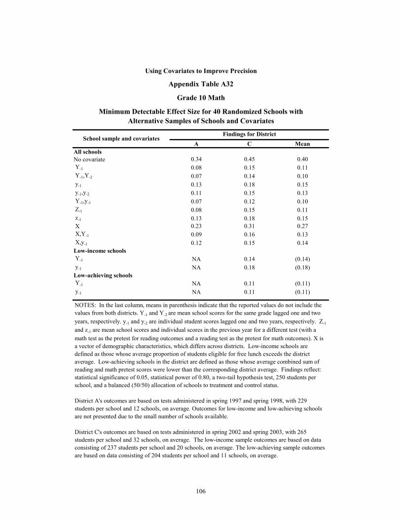
106
Appendix Table A32
Grade 10 Math
Minimum Detectable Effect Size for 40 Randomized Schools withAlternative Samples of Schools and Covariates
A C MeanAll schoolsNo covariate 0.34 0.45 0.40 Y-1 0.08 0.15 0.11 Y-1,Y-2 0.07 0.14 0.10 y-1 0.13 0.18 0.15 y-1,y-2 0.11 0.15 0.13 Y-1,y-1 0.07 0.12 0.10 Z-1 0.08 0.15 0.11 z-1 0.13 0.18 0.15 X 0.23 0.31 0.27 X,Y-1 0.09 0.16 0.13 X,y-1 0.12 0.15 0.14Low-income schools Y-1 NA 0.14 (0.14) y-1 NA 0.18 (0.18)Low-achieving schools Y-1 NA 0.11 (0.11) y-1 NA 0.11 (0.11)
School sample and covariatesFindings for District
Using Covariates to Improve Precision
NOTES: In the last column, means in parenthesis indicate that the reported values do not include the values from both districts. Y-1 and Y-2 are mean school scores for the same grade lagged one and two years, respectively. y-1 and y-2 are individual student scores lagged one and two years, respectively. Z-1
and z-1 are mean school scores and individual scores in the previous year for a different test (with a math test as the pretest for reading outcomes and a reading test as the pretest for math outcomes). X is a vector of demographic characteristics, which differs across districts. Low-income schools are defined as those whose average proportion of students eligible for free lunch exceeds the district average. Low-achieving schools in the district are defined as those whose average combined sum of reading and math pretest scores were lower than the corresponding district average. Findings reflect: statistical significance of 0.05, statistical power of 0.80, a two-tail hypothesis test, 250 students per school, and a balanced (50/50) allocation of schools to treatment and control status.
District A's outcomes are based on tests administered in spring 1997 and spring 1998, with 229 students per school and 12 schools, on average. Outcomes for low-income and low-achieving schools are not presented due to the small number of schools available.
District C's outcomes are based on tests administered in spring 2002 and spring 2003, with 265 students per school and 32 schools, on average. The low-income sample outcomes are based on data consisting of 237 students per school and 20 schools, on average. The low-achieving sample outcomes are based on data consisting of 204 students per school and 11 schools, on average.

107
Appendix Table A33
Grade 10 Math
Minimum Detectable Effect Size Ranges for 40 Randomized Schools with Alternative Samples
of Schools and Selected Covariates
(min, max) (min, max)All schools Y-1 (0.07, 0.08) (0.11, 0.18) y-1 (0.09, 0.16) (0.17, 0.19)Low-income schools Y-1 NA NA (0.12, 0.16) y-1 NA NA (0.16, 0.19)Low-achieving schools Y-1 NA NA (0.05, 0.13) y-1 NA NA (0.10, 0.11)
Using Covariates to Improve Precision
Findings for DistrictSchool sample and covariate A C
NOTES: Y-1 is the mean school score for the same grade lagged one year, and y-1 is the individual student score lagged one year. Low-income schools are defined as those whose average proportion of students eligible for free lunch exceeds the district average. Low-achieving schools in the district are defined as those whose average combined sum of reading and math pretest scores were lower than the corresponding district average. Findings reflect: statistical significance of 0.05, statistical power of 0.80, a two-tail hypothesis test, 250 students per school, and a balanced (50/50) allocation of schools to treatment and control status.
District A's outcomes are based on tests administered in spring 1997 and spring 1998, with 229 students per school and 12 schools, on average. Outcomes for low-income and low-achieving schools are not presented due to the small number of schools available.
District C's outcomes are based on tests administered in spring 2002 and spring 2003, with 265 students per school and 32 schools, on average. The low-income sample outcomes are based on data consisting of 237 students per school and 20 schools, on average. The low-achieving sample outcomes are based on data consisting of 204 students per school and 11 schools, on average.

108
Appendix Table A34
Grade 10 Math
Parameter Values for Selected Covariates
R2C R2
I R2C R2
I
Y-1 0.97 0.00 0.91 0.00Y-2 0.90 0.00 0.86 0.00Y-3 NA NA 0.82 0.00Y-1, Y-2 0.98 0.00 0.92 0.00Y-2, Y-3 NA NA 0.86 0.00
y-1 0.86 0.47 0.85 0.39y-2 0.82 0.39 0.80 0.35y-3 NA NA 0.80 0.32y-1, y-2 0.91 0.52 0.90 0.46y-2, y-3 NA NA 0.84 0.38
Y-1, y-1 0.97 0.47 0.93 0.39Z-1 0.97 0.00 0.91 0.00z-1 0.86 0.47 0.85 0.39X 0.55 0.15 0.55 0.16X, Y-1 0.95 0.15 0.89 0.16X, y-1 0.89 0.49 0.89 0.42
Other covariates
Using Covariates to Improve Precision
School-level pretests only
Student-level pretests only
Proportion of variance reduced (R2C and R2
I)
0.13 0.25Intra-class correlation with no covariates (ρ)
CovariatesA C
Parameters for District
NOTES: Y-1, Y-2, and Y-3 are mean school scores for the same grade lagged one, two, and threeyears, respectively. y-1, y-2, and y-3 are individual student scores lagged one, two, and three years, respectively. X is a vector of demographic characteristics, which differs across districts. Z-1 and z-1 are mean school scores and individual scores in the previous year for a different test (with a math test as the pretest for reading outcomes and a reading test as the pretest for math outcomes). R2
C and R2I are the average proportion of the school-level variance and the student-
level variance reduced by the covariates, respectively. The averages are computed as the meanof the corresponding district-level parameters. Nonzero estimates for R2
I with school-level covariates only are set equal to zero. See text for more details.
District A's outcomes are based on tests administered in spring 1997 and spring 1998, with 229students per school and 12 schools, on average. District C's outcomes are based on tests administered in spring 2002 and spring 2003, with 265 students per school and 32 schools, on average.

109
Appendix Table A35
Grade 10 Math
Parameter Ranges for Alternative School Samples and Selected Covariates
(min, max) (min, max) (min, max) (min, max)All schoolsρ (0.13, 0.14) (0.25, 0.25)R2
C (0.96, 0.99) (0.78, 0.95) (0.86, 0.95) (0.83, 0.86)
R2I (0.00, 0.00) (0.45, 0.49) (0.00, 0.00) (0.36, 0.43)
ρ NA NA (0.11, 0.13)R2
C NA NA NA NA (0.77, 0.89) (0.67, 0.75)
R2I NA NA NA NA (0.00, 0.00) (0.29, 0.36)
ρ NA NA (0.01, 0.03)R2
C NA NA NA NA (-0.13, 1.03) (0.31, 0.57)
R2I NA NA NA NA (0.00, 0.00) (0.26, 0.29)
y-1 Y-1 y-1
Low-achieving schools
(same for all models) (same for all models)
Y-1
(same for all models) (same for all models)
Low-income schools(same for all models) (same for all models)
Covariates
Parameters for District
Using Covariates to Improve Precision
School sample and parameters A C
NOTES: Y-1 is the mean school score for the same grade lagged one year, and y-1 is the individual student score lagged one year. ρ is the intra-class correlation for students within schools. R2
C and R2I
are the proportions of the school-level variance and the student-level variance reduced by the covariates, respectively. Nonzero estimates for R2
I with school-level covariates only are set equal to zero. See text for more details. Low-income schools are defined as those whose average proportion of students eligible for free lunch exceeds the district average. Low-achieving schools in the district are defined as those whose average combined sum of reading and math pretest scores were lower than the corresponding district average.
District A's outcomes are based on tests administered in spring 1997 and spring 1998, with 229 students per school and 12 schools, on average. Outcomes for low-income and low-achieving schools are not presented due to the small number of schools available.
District C's outcomes are based on tests administered in spring 2002 and spring 2003, with 265 students per school and 32 schools, on average. The low-income sample outcomes are based on data consisting of 237 students per school and 20 schools, on average. The low-achieving sample outcomes are based on data consisting of 204 students per school and 11 schools, on average.


111
Earlier MDRC Working Papers on Research Methodology Sample Design for an Evaluation of the Reading First Program 2003. Howard Bloom Intensive Qualitative Research Challenges, Best Uses, and Opportunities 2003. Alissa Gardenhire, Laura Nelson Exploring the Feasibility and Quality of Matched Neighborhood Research Designs 2003. David Seith, Nandita Verma, Howard Bloom, George Galster Can Nonexperimental Comparison Group Methods Match the Findings from a Random Assignment Evaluation of Mandatory Welfare-to-Work Programs? 2002. Howard Bloom, Charles Michalopoulos, Carolyn Hill, Ying Lei Using Instrumental Variables Analysis to Learn More from Social Policy Experiments 2002. Lisa Gennetian, Johannes Bos, Pamela Morris Using Place-Based Random Assignment and Comparative Interrupted Time-Series Analysis to Evaluate the Jobs-Plus Employment Program for Public Housing Residents 2002. Howard Bloom, James Riccio Measuring the Impacts of Whole School Reforms Methodological Lessons from an Evaluation of Accelerated Schools 2001. Howard Bloom A Meta-Analysis of Government-Sponsored Training Programs 2001. David Greenberg, Charles Michalopoulos, Philip Robins Modeling the Performance of Welfare-to-Work Programs The Effects of Program Management and Services, Economic Environment, and Client Characteristics 2001. Howard Bloom, Carolyn Hill, James Riccio A Regression-Based Strategy for Defining Subgroups in a Social Experiment 2001. James Kemple, Jason Snipes Explaining Variation in the Effects of Welfare-to-Work Programs 2001. David Greenberg, Robert Meyer, Charles Michalopoulos, Michael Wiseman Extending the Reach of Randomized Social Experiments New Directions in Evaluations of American Welfare-to-Work and Employment Initiatives 2001. James Riccio, Howard Bloom

112
The Politics of Random Assignment: Implementing Studies and Impacting Policy 2000. Judith Gueron Assessing the Impact of Welfare Reform on Urban Communities The Urban Change Project and Methodological Considerations 2000. Charles Michalopoulos, Joannes Bos, Robert Lalonde, Nandita Verma Building a Convincing Test of a Public Housing Employment Program Using Non-Experimental Methods Planning for the Jobs-Plus Demonstration 1999. Howard Bloom Estimating Program Impacts on Student Achievement Using “Short” Interrupted Time Series 1999. Howard Bloom Using Cluster Random Assignment to Measure Program Impacts Statistical Implications for the Evaluation of Education Programs 1999. Howard Bloom, Johannes Bos, Suk-Won Lee

About MDRC
MDRC is a nonprofit, nonpartisan social policy research organization dedicated to learn-ing what works to improve the well-being of low-income people. Through its research and the active communication of its findings, MDRC seeks to enhance the effectiveness of social and education policies and programs.
Founded in 1974 and located in New York City and Oakland, California, MDRC is best known for mounting rigorous, large-scale, real-world tests of new and existing policies and programs. Its projects are a mix of demonstrations (field tests of promising new pro-gram approaches) and evaluations of ongoing government and community initiatives. MDRC’s staff bring an unusual combination of research and organizational experience to their work, providing expertise on the latest in qualitative and quantitative methods and on program design, development, implementation, and management. MDRC seeks to learn not just whether a program is effective but also how and why the program’s effects occur. In addition, it tries to place each project’s findings in the broader context of related research — in order to build knowledge about what works across the social and education policy fields. MDRC’s findings, lessons, and best practices are proactively shared with a broad audience in the policy and practitioner community as well as with the general pub-lic and the media.
Over the years, MDRC has brought its unique approach to an ever-growing range of pol-icy areas and target populations. Once known primarily for evaluations of state welfare-to-work programs, today MDRC is also studying public school reforms, employment programs for ex-offenders and people with disabilities, and programs to help low-income students succeed in college. MDRC’s projects are organized into five areas:
• Promoting Family Well-Being and Child Development
• Improving Public Education
• Promoting Successful Transitions to Adulthood
• Supporting Low-Wage Workers and Communities
• Overcoming Barriers to Employment
Working in almost every state, all of the nation’s largest cities, and Canada and the United Kingdom, MDRC conducts its projects in partnership with national, state, and local governments, public school systems, community organizations, and numerous pri-vate philanthropies.