using conditional copula to estimate value at risk · 2018-11-07 · using conditional copula to...

Journal of Data Science 4(2006), 93-115

Using Conditional Copula to Estimate Value at Risk

Helder Parra Palaro and Luiz Koodi HottaState University of Campinas

Abstract: Value at Risk (VaR) plays a central role in risk management.There are several approaches for the estimation of VaR, such as histori-cal simulation, the variance-covariance (also known as analytical), and theMonte Carlo approaches. Whereas the first approach does not assume anydistribution, the last two approaches demand the joint distribution to beknown, which in the analytical approach is frequently the normal distri-bution. The copula theory is a fundamental tool in modeling multivariatedistributions. It allows the definition of the joint distribution through themarginal distributions and the dependence between the variables. Recentlythe copula theory has been extended to the conditional case, allowing the useof copulae to model dynamical structures. Time variation in the first andsecond conditional moments is widely discussed in the literature, so allow-ing the time variation in the conditional dependence seems to be natural.This work presents some concepts and properties of copula functions andan application of the copula theory in the estimation of VaR of a portfoliocomposed by Nasdaq and S&P500 stock indices.

Key words: Copula, multivariate distribution function, value-at-risk.

1. Introduction

Value at Risk (VaR) is probably the most popular risk measure, having a cen-tral role in risk management. Although VaR is a simple measure, it is not easilyestimated. There are several approaches for the estimation of VaR, such as thevariance-covariance (also known as analytical), the historical simulation and theMonte Carlo approaches. The analytical approach has been largely used afterthe publishing of the Riskmetrics methodology. This approach adopts the as-sumption of multivariate normality of the joint distribution of the assets returns.In this case, the covariance matrix is a natural measure of dependence betweenthe assets and the variance is a good measure of risk. In finance the normalityis rarely an adequate assumption. For instance, Longin and Solnick (2001) andAng and Chen (2002) found evidence that asset returns are more highly corre-lated during volatile markets and during market downturns. The deviation from

94 Helder Parra Palaro and Luiz Koodi Hotta

normality could lead to an inadequate VaR estimate. In this case, the portfo-lio could be either riskier than desired or the financial institution unnecessarilyconservative.

The theory of copulae is a very powerful tool for modeling joint distribu-tions because it does not require the assumption of joint normality and allow usto decompose any n-dimensional joint distribution into its n marginal distribu-tions and a copula function. Conversely, a copula produces a multivariate jointdistribution combining the marginal distributions and the dependence betweenthe variables. Copulae have been broadly used in the statistical literature. Thebooks of Joe (1997) and Nelsen (1999) presented a good introduction to the cop-ula theory. Although copulae have been only recently used in the financial area,there are already several applications in this area. The papers of Bouye et al.(2000), Embrechts, McNeil and Straumann (2002) and Embrechts, Lindskog andMcNeil (2003) provided general examples of applications of copulae in finance.There also several particular applications. For instance, Cherubini and Luciano(2001) estimated the VaR using the Archimedean copula family and the histori-cal empirical distribution in the estimation of marginal distributions; Rockingerand Jondeau (2001) used the Plackett copula with GARCH process with innova-tions modeled by the Student-t asymmetrical generalized distribution of Hansen(1994) and proposed a new measure of conditional dependence; Georges (2001)used the normal copula to model options time of exercise and for derivative pric-ing; Meneguzzo and Vecchiato (2002) used copulae for modeling the risk of creditderivatives; and Fortin and Kuzmics (2002) used convex linear combinations ofcopulae for estimating the VaR of a portfolio composed by the FSTE and DAXstock indices; and Embrechts, McNeil and Straumann (2002) and Embrechts, Ho-ing and Juri (2003) used copulae to model extreme value and risk limits. Theserecently published papers show the wide range of copula applications in finance.

The recent extension of the unconditional copula theory to the conditionalcase has been used by Patton (2003a) to model time-varying conditional depen-dence. Time variation in the first and second conditional moments is widelydiscussed in the statistical literature, so allowing the temporal variation in theconditional dependence in time series seems to be natural.

In this paper we discuss the application of conditional copula in estimatingthe VaR of a portfolio with two assets. The paper is organized as follow. Section2 defines copula and presents Sklar’s theorem. The copulae families used in thiswork are presented in Section 3 while Section 4 discusses some inference methodsfor copulae, like estimation and model selection. Finally, Section 5 applies themethod to a portfolio composed by two assets (the Nasdaq and the S&P500stock indices). After modeling and estimating the parameters by the InferenceFunction for Margins method, we used out-of-sample simulation techniques to

Using Conditional Copula to Estimate Value at Risk 95

test the accuracy of the VaR estimates. We compared the results obtained usingtraditional approaches to estimate VaR, like the Exponentially Weighted MovingAverages, the historical simulation, and univariate and bivariate GARCH models.

2. Introduction

According to Nelsen (1999, pg.1), copulae can be seen from two points ofview: “From one point of view, copulas are functions that join or couple mul-tivariate distribution functions to their one-dimensional marginal distributionfunctions. Alternatively, copulas are multivariate distribution functions whoseone-dimensional margins are uniform on the interval (0,1)”.

2.1 Definition

In this section we give the general definition of copulae and a equivalentdefinition for the random variable context.

For simplicity purposes, throughout this paper we treat only the bivariatecase, but the extension for higher dimensions is straightforward (see, for instance,Nelsen (1999) and Patton (2003a)).

Definition 2.1 A 2-dimensional copula function (or briefly a copula) is afunction C, whose domains is [0, 1]2 and whose range is [0, 1] with the followingproperties:

1. C(x) = 0 for all x ∈ [0, 1]2 when at least one element of x is 0;

2. C(x1, 1) = C(1, x2) = 1 for all (x1, x2) ∈ [0, 1]2;

3. for all (a1, a2), (b1, b2) ∈ [0, 1]2 with a1 ≤ b1 and a2 ≤ b2 , we have :

VC([a, b]) = C(a2, b2) − C(a1, b2) − C(a2, b1) + C(a1, b1) ≥ 0

Hence any bivariate distribution function whose margins are standard uni-form distributions is a copula.

Definition 2.2 The copula function C is a copula for the random vectorX = (X1,X2)t, if it is the joint distribution function of the random vectorU = (U1, U2)t where Ui = Fi(Xi), and Fi are the marginal distribution func-tions of Xi, i = 1, 2.

This imply that:H(x1, x2) = C(F1(x1), F2(x2)),


where H is the joint distribution function of (X1,X2). If F1 and F2 are continuousthen the copula C is unique. Thus we can interpret a copula as a function whichlinks the marginal distributions of a random vector to its joint distribution.

2.2 Sklar theorem

The next theorem is a key result in the theory of copulae :

Theorem 2.1 (Sklar Theorem) Let H be a 2-dimensional joint distributionfunction with marginal distributions F1, F2. Then there exists a copula C suchthat for all x ∈ �n,

H(x1, x2) = C(F1(x1), F2(x2)). (2.1)

If F1, F2 are continuous, then C is unique; otherwise, C is uniquely determinedon Ran(F1) × Ran(F2). Conversely, if C is a copula and F1, F2 are distributionfunctions, then the function H defined by (2.1) is a joint distribution functionwith margins F1 and F2.

The proof can be found in Nelsen (1999, p. 18).It is the converse of the Sklar’s theorem that is most interesting for modeling

multivariate distributions in finance. It implies that we may link any group ofn univariate distributions, of any type (not necessarily from the same family),with any copula and we will have defined a valid multivariate distribution. Theusefulness of this result stems from the fact that while in economics and statisticsliterature we have a large set of flexible parametric univariate distributions avail-able, the set of parametric multivariate distributions available is much smaller.According to Patton (2003a), referring to finance data, “Decomposing the multi-variate distribution into the marginal distributions and the copula allows for theconstruction of better models of the individual variables than would be possibleif we constrained ourselves to look only at existing multivariate distributions”.

Patton (2003a) extended and proved the validity of the Sklar’s theorem forthe conditional case. In this extension the conditioning variable(s) W must bethe same for the marginal distributions and the copula.

For the definition of copulae for the general case (n > 2) and for more details,look at Nelsen (1999), Bouye et al. (2000) and Patton (2003a).

3. Some Families of Copulae

In this section we present the three families of copulae used in this work :Student-t, Plackett, and symmetrized of Joe-Clayton copulae.


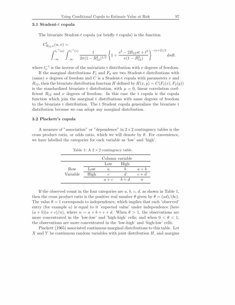
3.1 Student-t copula

The bivariate Student-t copula (or briefly t copula) is the function

CtR12,ν(u, v) =∫ t−1

ν (u)

−∞

∫ t−1ν (v)

−∞

12π(1 − R2

12)1/2

{1 +

s2 − 2R12st + t2

ν(1 − R212)

}−(ν+2)/2

dsdt.

where t−1ν is the inverse of the univariate t distribution with ν degrees of freedom.

If the marginal distributions F1 and F2 are two Student-t distributions with(same) ν degrees of freedom and C is a Student-t copula with parameters ν andR12, then the bivariate distribution function H defined by H(x, y) = C(F1(x), F2(y))is the standardized bivariate t distribution, with µ = 0, linear correlation coef-ficient R12 and ν degrees of freedom. In this case the t copula is the copulafunction which join the marginal t distributions with same degrees of freedomto the bivariate t distribution. The t Student copula generalizes the bivariate tdistribution because we can adopt any marginal distribution.

3.2 Plackett’s copula

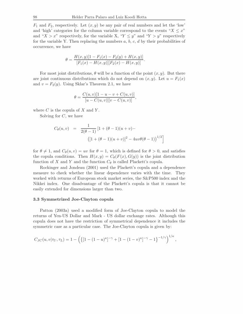
A measure of ”association” or ”dependence” in 2×2 contingency tables is thecross product ratio, or odds ratio, which we will denote by θ. For convenience,we have labelled the categories for each variable as ‘low’ and ‘high’.

Table 1: A 2 × 2 contingency table.

Column variableLow High

Row Low a b a + bVariable High c d c + d

a + c b + d n

If the observed count in the four categories are a, b, c, d, as shown in Table 1,then the cross product ratio is the positive real number θ given by θ = (ad)/(bc).The value θ = 1 corresponds to independence, which implies that each ’observed’entry (for example a) is equal to it ’expected value’ under independence (here(a + b)(a + c)/n), where n = a + b + c + d. When θ > 1, the observations aremore concentrated in the ’low-low’ and ’high-high’ cells; and when 0 < θ < 1,the observations are more concentrated in the ‘low-high’ and ‘high-low’ cells.

Plackett (1965) associated continuous marginal distributions to this table. LetX and Y be continuous random variables with joint distribution H, and margins


F1 and F2, respectively. Let (x, y) be any pair of real numbers and let the ‘low’and ‘high’ categories for the column variable correspond to the events “X ≤ x”and “X > x” respectively, for the variable X, “Y ≤ y” and “Y > y” respectivelyfor the variable Y. Then replacing the numbers a, b, c, d by their probabilities ofoccurrence, we have

θ =H(x, y)[1 − F1(x) − F2(y) + H(x, y)][F1(x) − H(x, y)][F2(x) − H(x, y)]

.

For most joint distributions, θ will be a function of the point (x, y). But thereare joint continuous distributions which do not depend on (x, y). Let u = F1(x)and v = F2(y). Using Sklar’s Theorem 2.1, we have

θ =C(u, v)[1 − u − v + C(u, v)][u − C(u, v)][v − C(u, v)]

,

where C is the copula of X and Y .Solving for C, we have

Cθ(u, v) =1

2(θ − 1)[1 + (θ − 1)(u + v)−

([1 + (θ − 1)(u + v)]2 − 4uvθ(θ − 1)

)1/2]

for θ �= 1, and Cθ(u, v) = uv for θ = 1, which is defined for θ > 0, and satisfiesthe copula conditions. Then H(x, y) = Cθ(F (x), G(y)) is the joint distributionfunction of X and Y and the function Cθ is called Plackett’s copula.

Rockinger and Jondeau (2001) used the Plackett’s copula and a dependencemeasure to check whether the linear dependence varies with the time. Theyworked with returns of European stock market series, the S&P500 index and theNikkei index. One disadvantage of the Plackett’s copula is that it cannot beeasily extended for dimensions larger than two.

3.3 Symmetrized Joe-Clayton copula

Patton (2003a) used a modified form of Joe-Clayton copula to model thereturns of Yen-US Dollar and Mark - US dollar exchange rates. Although thiscopula does not have the restriction of symmetrical dependence it includes thesymmetric case as a particular case. The Joe-Clayton copula is given by:

CJC(u, v|τU , τL) = 1 −({

[1 − (1 − u)κ]−γ + [1 − (1 − v)κ]−γ − 1}−1/γ

)1/κ,


where

κ = 1/log2(2 − τU )γ = −1/log2(τL)

τU ∈ (0, 1), τL ∈ (0, 1).

This copula has two parameters, τU and τL, which are the coefficients of upperand low tail dependence, respectively (see Patton (2003a)). The Joe-Claytoncopula still has a slight asymmetry when τU = τL, which is not convenient. Inorder to overcome this problem we have a modified form of the copula, known assymmetrized Joe-Clayton copula (SJC) which is given by:

CSJC(u, v|τU , τL) =0.5 CJC(u, v|τU , τL) + 0.5 CJC(1 − u, 1 − v|τL, τU ) + u + v − 1,

which is symmetric when τU = τL.

4. Statistical Inference of Copulae

Let (X1,X2), be a vector of two random variables with joint distributionfunction H and marginal distribution functions F1 and F2 respectively. Eachmarginal distribution function depends only on the parameter ϑi. Denote theunknown vector of parameters by ϑ = (ϑ1, ϑ2, θ), where θ is the vector of pa-rameters of the n-dimensional copula {Cθ, θ ∈ Θ} and Cθ is completely knownexcept for the parameter θ. Suppose that {(x1, t, x2, t)}T

t=1 is a sample of size T.Hence we have by Sklar’s theorem:

H(x1, x2) = C(F1(x1;ϑ1), F2(x2;ϑ2); θ). (4.1)

Thus the joint distribution function H is completely specified by the parametervector ϑ = (ϑ1, ϑ2, θ).

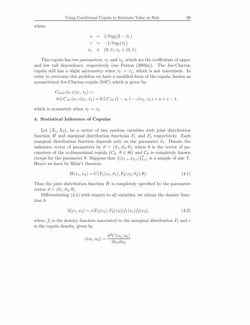
Differentiating (4.1) with respect to all variables, we obtain the density func-tion h

h(x1, x2) = c(F1(x1), F2(x2))f1(x1)f2(x2), (4.2)

where fi is the density function associated to the marginal distribution Fi and cis the copula density, given by

c(u1, u2) =∂2C(u1, u2)

∂u1∂u2.


4.1 Estimation

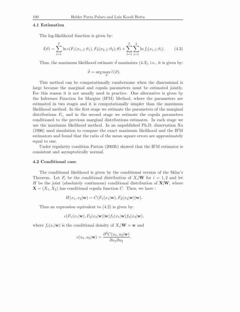
The log-likelihood function is given by:

l(ϑ) =T∑

t=1

ln c(F1(x1, t;ϑ1), F2(x2, t;ϑ2); θ) +T∑

t=1

2∑i=1

ln fi(xi, t;ϑi). (4.3)

Thus, the maximum likelihood estimate ϑ maximizes (4.3), i.e., it is given by:

ϑ = arg maxϑ

l (ϑ).

This method can be computationally cumbersome when the dimensional islarge because the marginal and copula parameters must be estimated jointly.For this reason it is not usually used in practice. One alternative is given bythe Inference Function for Margins (IFM) Method, where the parameters areestimated in two stages and it is computationally simpler than the maximumlikelihood method. In the first stage we estimate the parameters of the marginaldistributions Fi, and in the second stage we estimate the copula parametersconditioned to the previous marginal distributions estimates. In each stage weuse the maximum likelihood method. In an unpublished Ph.D. dissertation Xu(1996) used simulation to compare the exact maximum likelihood and the IFMestimators and found that the ratio of the mean square errors are approximatelyequal to one.

Under regularity condition Patton (2003b) showed that the IFM estimator isconsistent and asymptotically normal.

4.2 Conditional case

The conditional likelihood is given by the conditional version of the Sklar’sTheorem. Let Fi be the conditional distribution of Xi|W for i = 1, 2 and letH be the joint (absolutely continuous) conditional distribution of X|W, whereX = (X1,X2) has conditional copula function C. Then, we have :

H(x1, x2|w) = C(F1(x1|w), F2(x2|w)|w).

Thus an expression equivalent to (4.2) is given by:

c(F1(x1|w), F2(x2|w)|w)f1(x1|w)f2(x2|w),

where fi(xi|w) is the conditional density of Xi|W = w and

c(u1, u2|w) =∂2C(u1, u2|w)

∂u1∂u2.


The log-likelihood expression is equivalent to (4.3) :

l(ϑ) =T∑

t=1

ln c(F1(x1, t;ϑ1|wt), ..., Fn(xn, t;ϑn|wt); θ|wt) +

T∑t=1

2∑i=1

ln fi(xi, t;ϑi|wt),

and we can use all the previous methods to estimate the parameters.

4.3 Empirical Copula

The empirical copula C is defined as:

C

(t1T

,t2T

)=

1T

T∑t=1

1[x1, t≤x1(t1),x2, t≤x2(t2)], (4.4)

where 1 is the indicator function, xi, (tj), i = 1, 2, j = 1, 2 are the tj-th orderstatistics of the i-th variable and t1, t2 ∈ {1, ..., T}. Therefore the empiricalcopula is the proportion of elements from the sample that satisfies x1, t ≤ x1, (t1)

and x2, t ≤ x2, (t2).

4.4 Selection of the copula function

The quadratic distance between two copulae C1 and C2 in a (finite) set ofbivariate points A = {a1,a2, ...,am} is defined as:

d (C1, C2) =

[m∑

i=1

(C1 (ai) − C2 (ai))2

]1/2

. (4.5)

Let {Ck}1≤k≤K be the set of copulae under consideration. One criterion isto select the copula Ck which minimizes the quadratic distance between Ck, theestimated copula, and the empirical copula C, defined by (4.4), in the regionof interest. For instance, when selecting a model in order to estimate the VaR,the region of interest should be the lower tail. We will use this region in theSubsection 5.5.

Another suggestion is to use a criterion like Akaike’s information criterion(AIC) (Akaike, 1973) which is defined as

AIC(M) = −2 log-likelihood(θ, ϑ) + 2 M,


where M is the number of parameters being estimated and hat denotes the max-imum likelihood estimates. M and the parameters estimated depend on the se-lection approach. When we are selecting the copula function, M is the number ofthe copula parameters if the models for the marginal distributions are consideredas known. Smith(2003) used this criterion for copula selection.

5. Application

5.1 Value at risk

In 1994 the American bank JP Morgan published a risk control method knowsas Riskmetrics, based mainly on a parameter named Value at Risk.

The Value at Risk is a forecast of a given percentile, usually in the lower tail,of the distribution of returns on a portfolio over some period ∆t. The VaR of aportfolio at time t, with confidence level 1 − α, where α ∈ (0, 1) is defined as:

V aRt(α) = inf{s : Fp, t(s) ≥ α},

where Fp, t is the distribution function of the portfolio return Xp, t at time t(return from t−∆t to t). Equivalently, we have P (Xp, t ≤ V aRt(α)) = α at timet. This means that we are 100(1 − α)% confident that the loss in the period ∆t

will not be larger than the VaR.VaR is being used for several needs; risk reporting, risk limits, regulatory

capital, internal capital allocation and performance measurement. An inade-quate VaR estimation can lead to a underestimation of the risk incurred. On theother hand, a conservative position due to overestimation of the VaR would, forinstance, not consider certain risk controlled positions.

We are going to work with one-day period VaR. Consider the case of a portfoliocomposed by two assets, with returns at t − th day, denoted as X1, t and X2, t

respectively. The portfolio return, denoted as Xp, t is approximately equal toω1X1, t + ω2X2, t, where ω1 and ω2 are the portfolio weighs of assets 1 and 2. Forthe VaR estimation, we could study the distribution of the univariate portfolioreturn series, or the bivariate distribution of the vector (X1, t,X2, t).

In this paper we use copula theory to model the vector (X1, t,X2, t). Themodeling is done in the following sequence :

• An exploratory data analysis is done in Subsection 5.2.

• The general model is presented in Subsection 5.3. The model selection andestimation is done in two steps :

ARMA-GARCH models are fitted for each return series in Subsection5.4.


The bivariate distribution of the ARMA-GARCH models is modeled bythree copulae families in Subsection 5.5. They are fitted for the innovationsestimated in Subsection 5.4.

• The fitted models are used to estimate the VaR. A backtesting is used totest the VaR estimates. This is done in Subsection 5.6.

• The best copula model is compared to traditional VaR estimation methodsin Subsection 5.7.

5.2 Data description

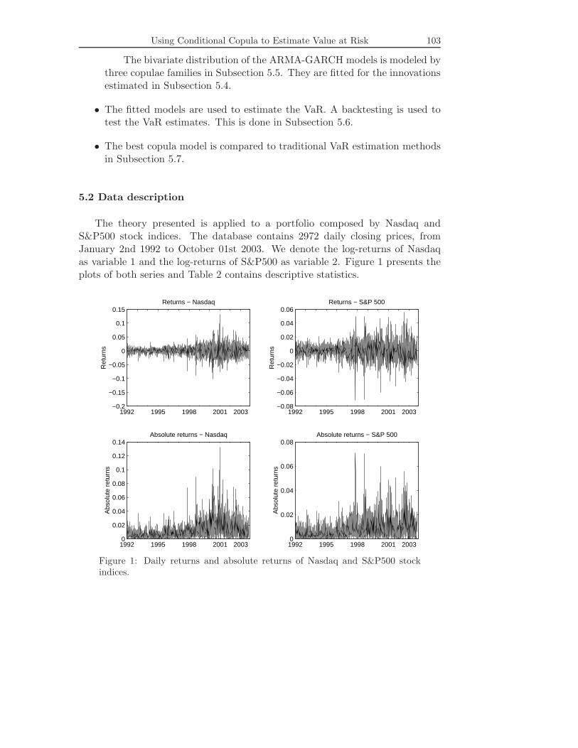
The theory presented is applied to a portfolio composed by Nasdaq andS&P500 stock indices. The database contains 2972 daily closing prices, fromJanuary 2nd 1992 to October 01st 2003. We denote the log-returns of Nasdaqas variable 1 and the log-returns of S&P500 as variable 2. Figure 1 presents theplots of both series and Table 2 contains descriptive statistics.

1992 1995 1998 2001 2003−0.2

−0.15

−0.1

−0.05

0

0.05

0.1

0.15Returns − Nasdaq

Ret

urns

1992 1995 1998 2001 2003−0.08

−0.06

−0.04

−0.02

0

0.02

0.04

0.06Returns − S&P 500

Ret

urns

1992 1995 1998 2001 20030

0.02

0.04

0.06

0.08

0.1

0.12

0.14Absolute returns − Nasdaq

Abs

olut

e re

turn

s

1992 1995 1998 2001 20030

0.02

0.04

0.06

0.08Absolute returns − S&P 500

Abs

olut

e re

turn

s

Figure 1: Daily returns and absolute returns of Nasdaq and S&P500 stockindices.


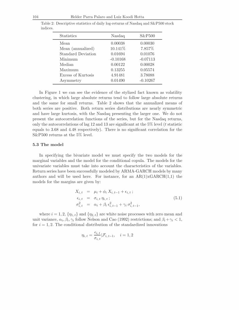
Table 2: Descriptive statistics of daily log-returns of Nasdaq and S&P500 stockindices.

Statistics Nasdaq S&P500

Mean 0.00038 0.00030Mean (annualized) 10.141% 7.857%Standard Deviation 0.01694 0.01076Minimum -0.10168 -0.07113Median 0.00122 0.00028Maximum 0.13255 0.05574Excess of Kurtosis 4.91481 3.78088Asymmetry 0.01490 -0.10267

In Figure 1 we can see the evidence of the stylized fact known as volatilityclustering, in which large absolute returns tend to follow large absolute returnsand the same for small returns. Table 2 shows that the annualized means ofboth series are positive. Both return series distributions are nearly symmetricand have large kurtosis, with the Nasdaq presenting the larger one. We do notpresent the autocorrelation functions of the series, but for the Nasdaq returns,only the autocorrelations of lag 12 and 13 are significant at the 5% level (t statisticequals to 3.68 and 4.48 respectively). There is no significant correlation for theS&P500 returns at the 5% level.

5.3 The model

In specifying the bivariate model we must specify the two models for themarginal variables and the model for the conditional copula. The models for theunivariate variables must take into account the characteristics of the variables.Return series have been successfully modeled by ARMA-GARCH models by manyauthors and will be used here. For instance, for an AR(1)xGARCH(1,1) themodels for the margins are given by:

Xi, t = µi + φi Xi, t−1 + εi, t ;εi, t = σi, t ηi, t ; (5.1)σ2

i, t = αi + βi ε2i, t−1 + γi σ2

i, t−1,

where i = 1, 2, {η1, t} and {η2, t} are white noise processes with zero mean andunit variance, αi, βi, γi follow Nelson and Cao (1992) restrictions; and βi +γi < 1,for i = 1, 2. The conditional distribution of the standardized innovations

ηi, t =εi, t

σi, t|Fi, t−1, i = 1, 2


was modeled by standard normal and standard t distributions. We denoted thesemodels, respectively by GARCH-N, GARCH-t. The distribution of the innovationvector ηt = (η1,t, η2,t) is modeled by copula. This approach was applied, forinstance, by Dias and Embrechts (2003) and Patton (2003a). The ARMA ×GARCH models work as a filter in order to have innovation processes, which areserially independent.

In order to apply the copula models we need to specify the conditional marginaldistributions. Additionally to the normal and t distributions we are also goingto use the empirical distribution of the residuals (estimates of the standardizedinnovations). According to the IFM method the selected copula functions willbe fitted to these residuals series. The estimation of the models is done in thefollowing subsections.

5.4 Modeling the marginal distributions

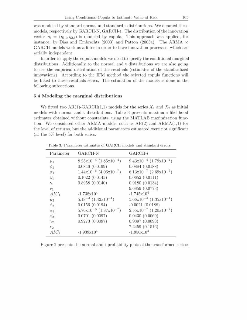
We fitted two AR(1)-GARCH(1,1) models for the series X1 and X2 as initialmodels with normal and t distributions. Table 3 presents maximum likelihoodestimates obtained without constraints, using the MATLAB maximization func-tion. We considered other ARMA models, such as AR(2) and ARMA(1,1) forthe level of returns, but the additional parameters estimated were not significant(at the 5% level) for both series.

Table 3: Parameter estimates of GARCH models and standard errors.

Parameter GARCH-N GARCH-t

µ1 8.25x10−4 (1.85x10−4) 9.43x10−4 (1.79x10−4)φ1 0.0846 (0.0199) 0.0884 (0.0188)α1 1.44x10−6 (4.06x10−7) 6.13x10−7 (2.69x10−7)β1 0.1022 (0.0145) 0.0652 (0.0111)γ1 0.8958 (0.0140) 0.9180 (0.0134)ν1 9.6859 (0.0773)AIC1 -1.738x104 -1.745x104

µ2 5.18−4 (1.42x10−4) 5.66x10−4 (1.35x10−4)φ2 0.0156 (0.0194) -0.0021 (0.0188)α2 5.76x10−6 (1.87x10−7) 2.55x10−7 (1.20x10−7)β2 0.0701 (0.0097) 0.0430 (0.0069)γ2 0.9273 (0.0097) 0.9397 (0.0093)ν2 7.2459 (0.1516)AIC2 -1.939x104 -1.950x104

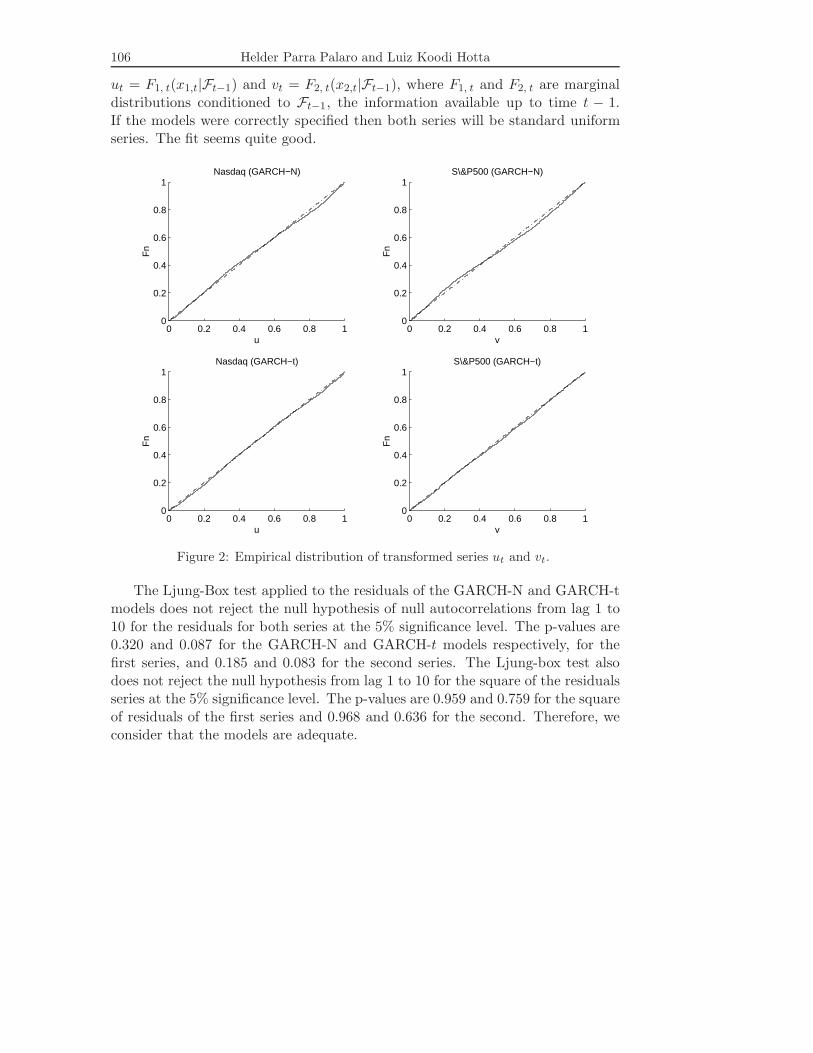
Figure 2 presents the normal and t probability plots of the transformed series:


ut = F1, t(x1,t|Ft−1) and vt = F2, t(x2,t|Ft−1), where F1, t and F2, t are marginaldistributions conditioned to Ft−1, the information available up to time t − 1.If the models were correctly specified then both series will be standard uniformseries. The fit seems quite good.

0 0.2 0.4 0.6 0.8 10

0.2

0.4

0.6

0.8

1Nasdaq (GARCH−N)

u

Fn

0 0.2 0.4 0.6 0.8 10

0.2

0.4

0.6

0.8

1Nasdaq (GARCH−t)

u

Fn

0 0.2 0.4 0.6 0.8 10

0.2

0.4

0.6

0.8

1S\&P500 (GARCH−N)

v

Fn

0 0.2 0.4 0.6 0.8 10

0.2

0.4

0.6

0.8

1S\&P500 (GARCH−t)

v

Fn

Figure 2: Empirical distribution of transformed series ut and vt.

The Ljung-Box test applied to the residuals of the GARCH-N and GARCH-tmodels does not reject the null hypothesis of null autocorrelations from lag 1 to10 for the residuals for both series at the 5% significance level. The p-values are0.320 and 0.087 for the GARCH-N and GARCH-t models respectively, for thefirst series, and 0.185 and 0.083 for the second series. The Ljung-box test alsodoes not reject the null hypothesis from lag 1 to 10 for the square of the residualsseries at the 5% significance level. The p-values are 0.959 and 0.759 for the squareof residuals of the first series and 0.968 and 0.636 for the second. Therefore, weconsider that the models are adequate.


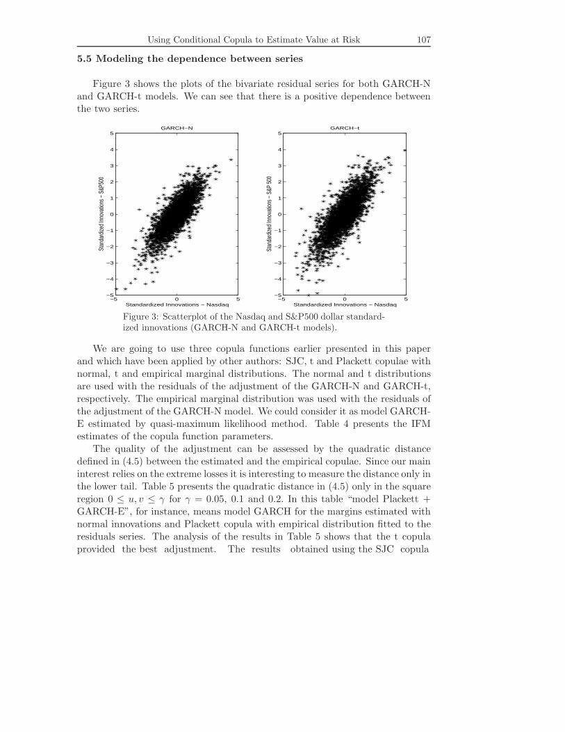
5.5 Modeling the dependence between series

Figure 3 shows the plots of the bivariate residual series for both GARCH-Nand GARCH-t models. We can see that there is a positive dependence betweenthe two series.

−5 0 5−5

−4

−3

−2

−1

0

1

2

3

4

5GARCH−N

Standardized Innovations − Nasdaq

Stan

dard

ized

Inno

vatio

ns −

S&P

500

−5 0 5−5

−4

−3

−2

−1

0

1

2

3

4

5GARCH−t

Standardized Innovations − Nasdaq

Stan

dard

ized

Inno

vatio

ns −

S&P

500

Figure 3: Scatterplot of the Nasdaq and S&P500 dollar standard-ized innovations (GARCH-N and GARCH-t models).

We are going to use three copula functions earlier presented in this paperand which have been applied by other authors: SJC, t and Plackett copulae withnormal, t and empirical marginal distributions. The normal and t distributionsare used with the residuals of the adjustment of the GARCH-N and GARCH-t,respectively. The empirical marginal distribution was used with the residuals ofthe adjustment of the GARCH-N model. We could consider it as model GARCH-E estimated by quasi-maximum likelihood method. Table 4 presents the IFMestimates of the copula function parameters.

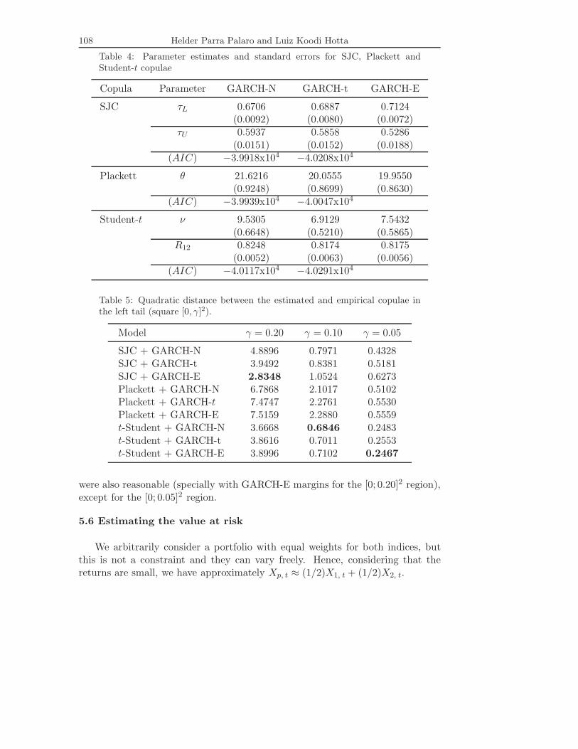
The quality of the adjustment can be assessed by the quadratic distancedefined in (4.5) between the estimated and the empirical copulae. Since our maininterest relies on the extreme losses it is interesting to measure the distance only inthe lower tail. Table 5 presents the quadratic distance in (4.5) only in the squareregion 0 ≤ u, v ≤ γ for γ = 0.05, 0.1 and 0.2. In this table “model Plackett +GARCH-E”, for instance, means model GARCH for the margins estimated withnormal innovations and Plackett copula with empirical distribution fitted to theresiduals series. The analysis of the results in Table 5 shows that the t copulaprovided the best adjustment. The results obtained using the SJC copula


Table 4: Parameter estimates and standard errors for SJC, Plackett andStudent-t copulae

Copula Parameter GARCH-N GARCH-t GARCH-E

SJC τL 0.6706 0.6887 0.7124(0.0092) (0.0080) (0.0072)

τU 0.5937 0.5858 0.5286(0.0151) (0.0152) (0.0188)

(AIC) −3.9918x104 −4.0208x104

Plackett θ 21.6216 20.0555 19.9550(0.9248) (0.8699) (0.8630)

(AIC) −3.9939x104 −4.0047x104

Student-t ν 9.5305 6.9129 7.5432(0.6648) (0.5210) (0.5865)

R12 0.8248 0.8174 0.8175(0.0052) (0.0063) (0.0056)

(AIC) −4.0117x104 −4.0291x104

Table 5: Quadratic distance between the estimated and empirical copulae inthe left tail (square [0, γ]2).

Model γ = 0.20 γ = 0.10 γ = 0.05

SJC + GARCH-N 4.8896 0.7971 0.4328SJC + GARCH-t 3.9492 0.8381 0.5181SJC + GARCH-E 2.8348 1.0524 0.6273Plackett + GARCH-N 6.7868 2.1017 0.5102Plackett + GARCH-t 7.4747 2.2761 0.5530Plackett + GARCH-E 7.5159 2.2880 0.5559t-Student + GARCH-N 3.6668 0.6846 0.2483t-Student + GARCH-t 3.8616 0.7011 0.2553t-Student + GARCH-E 3.8996 0.7102 0.2467

were also reasonable (specially with GARCH-E margins for the [0; 0.20]2 region),except for the [0; 0.05]2 region.

5.6 Estimating the value at risk

We arbitrarily consider a portfolio with equal weights for both indices, butthis is not a constraint and they can vary freely. Hence, considering that thereturns are small, we have approximately Xp, t ≈ (1/2)X1, t + (1/2)X2, t.


In order to asses the accuracy of the VaR estimates we backtested the methodat 95%, 99% and 99.5 % confidence level by the following procedure. Since attime t you only know the data up to this point the VaR must be evaluated withthe model (AR(1) - GARCH(1,1) + copula) estimated using only information upto this time. After estimating the total model we can simulate from the estimatedcopula to have an estimate of the joint distribution of the vector of innovationsηt+1. Using model (5.1) we can have an estimate of the portfolio distribution andestimate the VaR. Since estimating the model and simulating from the copulacould be computationally too cumbersome we estimated the model only once atevery 50 observations because we did not expect to have large difference in theestimated models when modifying a fraction of the observations.

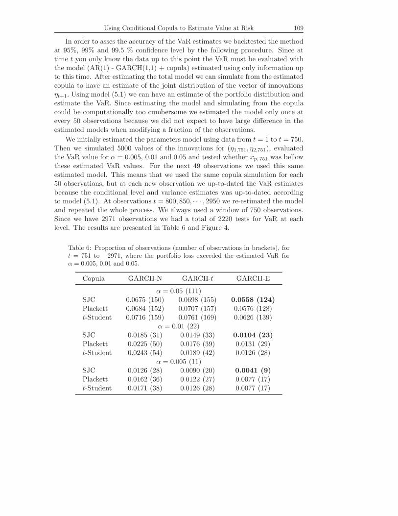
We initially estimated the parameters model using data from t = 1 to t = 750.Then we simulated 5000 values of the innovations for (η1,751, η2,751), evaluatedthe VaR value for α = 0.005, 0.01 and 0.05 and tested whether xp, 751 was bellowthese estimated VaR values. For the next 49 observations we used this sameestimated model. This means that we used the same copula simulation for each50 observations, but at each new observation we up-to-dated the VaR estimatesbecause the conditional level and variance estimates was up-to-dated accordingto model (5.1). At observations t = 800, 850, · · · , 2950 we re-estimated the modeland repeated the whole process. We always used a window of 750 observations.Since we have 2971 observations we had a total of 2220 tests for VaR at eachlevel. The results are presented in Table 6 and Figure 4.

Table 6: Proportion of observations (number of observations in brackets), fort = 751 to 2971, where the portfolio loss exceeded the estimated VaR forα = 0.005, 0.01 and 0.05.

Copula GARCH-N GARCH-t GARCH-E

α = 0.05 (111)SJC 0.0675 (150) 0.0698 (155) 0.0558 (124)Plackett 0.0684 (152) 0.0707 (157) 0.0576 (128)t-Student 0.0716 (159) 0.0761 (169) 0.0626 (139)




−0.05

0

0.05

Estimated VaR (SJC copula − GARCH−E margins)

Observation

Por

tfolio

ret

urn

/ VaR

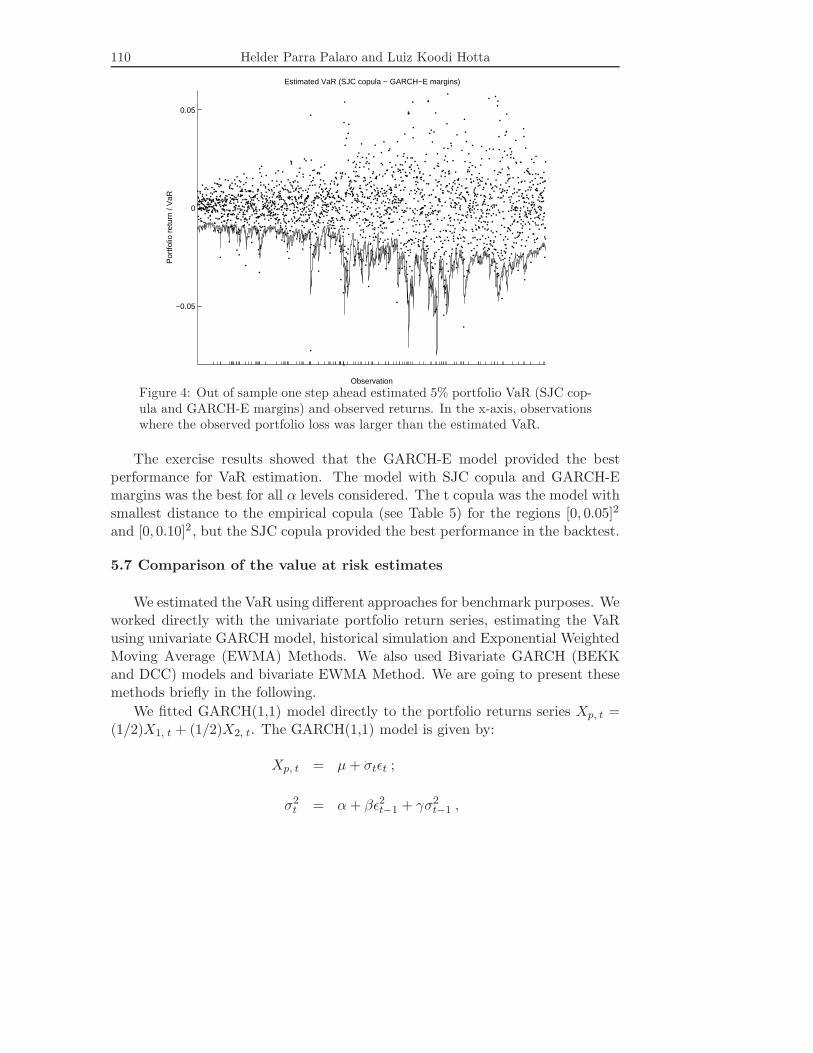
Figure 4: Out of sample one step ahead estimated 5% portfolio VaR (SJC cop-ula and GARCH-E margins) and observed returns. In the x-axis, observationswhere the observed portfolio loss was larger than the estimated VaR.

The exercise results showed that the GARCH-E model provided the bestperformance for VaR estimation. The model with SJC copula and GARCH-Emargins was the best for all α levels considered. The t copula was the model withsmallest distance to the empirical copula (see Table 5) for the regions [0, 0.05]2

and [0, 0.10]2 , but the SJC copula provided the best performance in the backtest.

5.7 Comparison of the value at risk estimates

We estimated the VaR using different approaches for benchmark purposes. Weworked directly with the univariate portfolio return series, estimating the VaRusing univariate GARCH model, historical simulation and Exponential WeightedMoving Average (EWMA) Methods. We also used Bivariate GARCH (BEKKand DCC) models and bivariate EWMA Method. We are going to present thesemethods briefly in the following.

We fitted GARCH(1,1) model directly to the portfolio returns series Xp, t =(1/2)X1, t + (1/2)X2, t. The GARCH(1,1) model is given by:

Xp, t = µ + σtεt ;

σ2t = α + βε2

t−1 + γσ2t−1 ,


where {εt} is a white noise process with zero mean and unit variance and α, β andγ follow the same restrictions given in model (5.1). We considered the Normaland t distributions for the innovations.

The EWMA method is generally used in the Riskmetrics methodology. Letσ2

p, t be the variance of the portfolio return in time t. The estimated variance,using data up to time t − 1, is given by :

σ2p, t/t−1 = (1 − λ)x2

p, t−1 + λσ2p, t−1/t−2 ,

where σ2p,(t+1)/t is the smoothed variance considering data up to time t .Consid-

ering the normal distribution, we have xp, t ∼ N (0, σ2p, t). The parameter λ is

re-estimated on each day t, minimizing the quantity

t−1∑i=50

(σ2p,(i+1)/i − x2

p,i+1)2.

We can also use the EWMA method in the bivariate case. In this case theestimated variances and covariance are given by :

σ21, t/t−1 = (1 − λ1)x2

1, t−1 + λ1σ21, t−1/t−2 ;

σ22, t/t−1 = (1 − λ2)x2

2, t−1 + λ2σ22, t−1/t−2 ;

σ12, t/t−1 = (1 − λ12)x1, t−1 x2, t−1 + λ12σ12, t−1/t−2 ,

where the optimal parameters λ1, λ2 and λ12 are obtained at every time t mini-mizing the quantities

t−1∑i=50

(σ21, (i+1)/i − x2

1, i+1)2,

t−1∑i=50

(σ22, (i+1)/i − x2

2, i+1)2, and

t−1∑i=50

(σ12, (i+1)/i − x21, i+1 x2

2, i+1)2

respectively. σ21, t/t−1, σ2

2, t/t−1 and σ12, t/t−1 are estimates of the bivariate covari-ance matrix and interpreted similarly to the univariate case.

We also considered a exponential smoothing for the returns mean, but theresults obtained were very close, so we maintained the model with zero means.

We also used the historical simulation approach. For this approach, considersome day t0. The estimated VaR for the day t0 + 1 with confidence level 1 − α


is given by the αt0-th order statistics of the sample of portfolio returns for t =1, ..., t0.

The first class of bivariate GARCH models used is the BEKK model (Engleand Kroner, 1995). Let

xt =(

x1, t

x2, t

), εt =

(ε1, t

ε2, t

), µ =

(µ1

µ2

),

A =(

a11 a12

a21 a22

), B =

(b11 b12

b21 b22

), C =

(c11 c12

0 c22

)and let

Σt =(

σ21, t σ12, t

σ12, t σ22, t

)= Cov [εt|�t−1] .

The BEKK model is given by :{xt = µ + εt ;Σt = C ′C + A′εt−1ε

′t−1A + B′Σt−1B .

We assumed that the innovations vector εt has conditionally a normal distributionN (0,Σt). The program used for the estimation was the SAS 8.2, proc VARMAX.

The second class of bivariate GARCH models used is the DCC one, proposedby Engle (2002). Let xi be the returns with mean equals zero, for i=1,...n. Theconditional correlation and variances are defined by :

σi, j, t = E [xi, t xj, t|�t−1] /√

E[x2

i, t|�t−1

]E

[x2

j, t|�t−1

].

Let σ2i, t = E

[x2

i, t|�t−1

]and ηi, t = xi, t/σi, t. So the correlation can be written as

σi, j, t = E [ηi, t ηj, t|�t−1]. Engle (2002) suggests estimating the GARCH processes

qi, j, t = σi, j + α(ηi, t−1 ηj, t−1 − σi, j) + β(qi, j, t−1 − σi, j)

for i, j = 1, ..., n and obtaining σi, j, t = qi, j, t/√

qi, i, t qj, j, t. We can interpretσi, j as the unconditional correlation between the innovations of the univariateGARCH models ηi, t ηj, t. Therefore the correlations and variances are modeledas GARCH processes with common parameters α and β, and with different un-conditional expected values σi, j.

We began the VaR estimation using data from t = 1 to t = 750. In thecase of the bivariate and univariate GARCH models the model parameters werere-estimated after each 50 returns, like before for copulae. For the EWMA andHistorical Simulation methods, the estimates were updated day by day fromt = 750 on.

Table 7 compares the benchmark models and the best model with copula(SJC copula with GARCH-E margins).


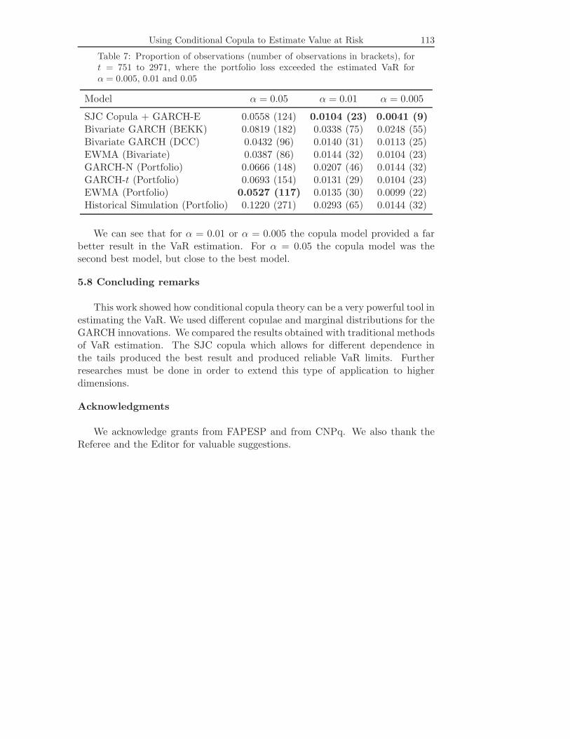
Table 7: Proportion of observations (number of observations in brackets), fort = 751 to 2971, where the portfolio loss exceeded the estimated VaR forα = 0.005, 0.01 and 0.05

Model α = 0.05 α = 0.01 α = 0.005

SJC Copula + GARCH-E 0.0558 (124) 0.0104 (23) 0.0041 (9)Bivariate GARCH (BEKK) 0.0819 (182) 0.0338 (75) 0.0248 (55)Bivariate GARCH (DCC) 0.0432 (96) 0.0140 (31) 0.0113 (25)EWMA (Bivariate) 0.0387 (86) 0.0144 (32) 0.0104 (23)GARCH-N (Portfolio) 0.0666 (148) 0.0207 (46) 0.0144 (32)GARCH-t (Portfolio) 0.0693 (154) 0.0131 (29) 0.0104 (23)EWMA (Portfolio) 0.0527 (117) 0.0135 (30) 0.0099 (22)Historical Simulation (Portfolio) 0.1220 (271) 0.0293 (65) 0.0144 (32)

We can see that for α = 0.01 or α = 0.005 the copula model provided a farbetter result in the VaR estimation. For α = 0.05 the copula model was thesecond best model, but close to the best model.

5.8 Concluding remarks

This work showed how conditional copula theory can be a very powerful tool inestimating the VaR. We used different copulae and marginal distributions for theGARCH innovations. We compared the results obtained with traditional methodsof VaR estimation. The SJC copula which allows for different dependence inthe tails produced the best result and produced reliable VaR limits. Furtherresearches must be done in order to extend this type of application to higherdimensions.

Acknowledgments

We acknowledge grants from FAPESP and from CNPq. We also thank theReferee and the Editor for valuable suggestions.


References

Akaike, H. (1973). Information theory and an extension of the maximum likelihood prin-ciple. Second International Symposium on Information Theory, 267-281, AkademiaiKiado, Budapest.

Ang, A. and J. Chen (2002). Asymmetric Correlations of Equity Portfolios, Journal ofFinancial Economics 63, 443-494.

Bouye, E., Durrleman, V., Nikeghbali, A., Riboulet, G. and Roncalli, T. (2000). Cop-ulas for finance, a reading guide and some applications. Working paper, FinancialEconometrics Research Center, City University, London.

Cherubini, U. and Luciano, E. (2001). Value at risk trade-off and capital allocationwith copulas. Economic Notes 30, 235-256.

Dias, A., and Embrechts, P. (2003). Dynamic copula models for multivariate high-frequency data in finance. Working Paper, ETH Zurich: Department of Mathe-matics.

Embrechts, P. and Hoing, A., Juri, A. (2003). Using copulae to bound the value-at-riskfor functions of dependent risks. Finance and Stochastics 7, 145-167.

Embrechts, P., Lindskog, F. and McNeil, A.J. (2003). Modelling dependence withcopulas and applications to risk management. In Handbook of Heavy Tailed Dis-tributions in Finance (Edited by S. T. Rachev), 329-384 Elsevier

Embrechts, P., McNeil, A. and Straumann, D. (2002). Correlation and dependence inrisk management: properties and pitfalls. In Risk Management Value at Risk andBeyond (Edited bu M. Dempster), 176-223. Cambridge University Press.

Engle, R. (2002). Dynamic conditional correlation - a simple class of multivariateGARCH. Journal of Business and Economics Statistics 20, 339-350.

Engle, R., Kroner, K. F. (1995). Multivariate simultaneous generalized ARCH. Econo-metric Theory 11, 122-150.

Fortin, I. and Kuzmics, C. (2002). Tail dependence in stock return pairs. InternationalJournal of Intelligent Systems in Accounting, Finance & Management 11, 89-107.

Georges, P., Lamy, A.G., Nicolas, E., Quibel, G. and Roncalli, T. (2001). Multivari-ate survival modelling: a unified approach with copulas. Working paper, CreditLyonnais, Paris.

Hansen, B. (1994). Autoregressive conditional density estimation. International Eco-nomic Review 35, 705-730.

Joe, H. (1997). Multivariate Models and Dependence Concepts. Chapman and Hall.

Kimberling, H. C. (1974). A probabilistic interpretation of complete monotonicity.Aequationes Mathematics 10, 152-164.


Longin, F. and Solnik, B. (2001). Extreme correlation of international equity markets.Journal of Finance 56, 649-676.

Mashal, R. and Zeevi, A. (2002). Beyond correlation : Extreme co-movements betweenfinancial assets. Working paper, Columbia University.

Meneguzzo, D. and Vecchiato, W. (2002). Copulas sensitivity in collaterized debt obli-gations and basket defaults swaps pricing and risk monitoring. Working paper,Veneto Banca.

Nelsen, R. B. (1999). Introduction to Copulas, Springer Verlag.

Nelson, D. B. and Cao, C. Q. (1992). Inequality constraints in the univariate GARCHmodel. Journal of Business and Economic Statistics 10, 229-235.

Patton, A. (2003a). Modelling asymmetric exchange rate dependence. Working paper,University of California, San Diego.

Patton, A. (2003b). Estimation of multivariate models for time series of possibly dif-ferent lengths. Working paper, University of California at San Diego.

Plackett, R. L. (1965). A class of bivariate distributions. Journal of American StatisticalAssociation 60, 516-522.

Rockinger, M. and Jondeau, E. (2001). Conditional dependency of financial series: anapplication of copulas. Working paper NER # 82, Banque de France. Paris.

Smith, M. (2003) Modelling sample selection using archimedean copulas. EconometricsJournal, 6, 99-123.

Xu, J. J. (1996). Statistical modelling and inference for multivariate and longitudinaldiscrete response data. PhD thesis, Statistics Department, University of BritishColumbia.

Received April 16, 2004; accepted September 27, 2004.

Helder Parra PalaroUniversity of CampinasDepartment of Statistics, CP 606513083-970, Campinas, SP, [email protected]

Luiz Koodi HottaUniversity of CampinasDepartment of Statistics, CP 606513083-970, Campinas, SP, [email protected].

using conditional copula to estimate value at risk · 2018-11-07 · using conditional copula to...

Documents