REPORT SNO 5213-2006

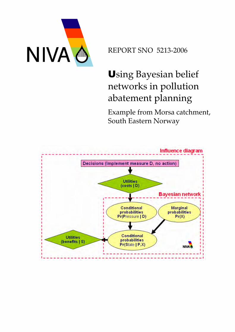
Using Bayesian belief networks in pollution abatement planning Example from Morsa catchment, South Eastern Norway

EutroBayes

Using Bayesian belief networks in pollution abatement planning

Example from Morsa catchment, South Eastern

Norway

NIVA 5213-2006

Preface

NIVA has been experimenting with the Bayesian network software Hugin Expert for nearly two years prior to the EutroBayes project, using existing data, models results and reports from the Morsa catchment. The work conducted during 2004-2005 owes thanks to partial funding from the BMW Project – “Benchmark Models for the Water Framework Directive” and the NOLIMP-WFD Project – “The North Sea Regional and Local Implementation of the Water Framework Directive”. The present report summarises some of the research challenges uncovered so far and will hopefully provide a starting point for researchers familiar with eutrophication issues who wish to know more about the potential and limitations of Bayesian networks in watershed management.

Oslo, May 2006

David N. Barton

NIVA 5213-2006

Contents

Summary 5

1. Introduction 6

2. Bayesian networks in river basin modelling and management 7

3. BN research challenges for NIVA 9

4. Case study site description 12

5. Methods and data 14

6. Results 19

7. REFERENCES 21

Appendix 1 – Conditional probability table illustrator 44

NIVA 5213-2006

5

Summary

A Bayesian belief network approach is used to conduct decision analysis of nutrient abatement measures in the Morsa catchment, South Eastern Norway, structuring available cost-effectiveness studies, eutrophication models and data in a DPSIR framework. Probability distributions for different nodes in the Bayesian network are derived from Monte Carlo uncertainty analysis of eutrophication models, parameter uncertainty derived from regression analyses and expert judgment. The report demonstrates that Bayesian belief networks can be used to conduct cost-effectiveness and benefit-cost analysis under uncertainty, responding to the economic analysis requirements of the EU Water Framework Directive (WFD). Furthermore, the ability to conduct forward (deductive) and backward (inductive) sensitivity analysis, as well as benefit-cost analysis of additional information (information analysis) in Bayesian networks is demonstrated. Information analysis, which uncovers which parts of the DPSIR ‘chain’ contribute most to uncertainty in decision-making, can be of use in optimising integrated environmental monitoring programmes in watershed management plans expected under the EU WFD. The report also raises a number of methodological questions regarding implementation of Bayesian networks in practice which are being addressed in ongoing NIVA projects (EUTROBAYES, Model-SIP).

NIVA 5213-2006

6

1. Introduction

The report documents NIVAs work with Bayesian belief networks in 2005, and implementaiton of these methodologies to pollution abatement planning in the Morsa catchment, Southern Norway, using Hugin Expert ® software. The report is based on an earlier model reported in Barton et al.(2006), which demonstrates the management problem structure as we had visualised it medio 2005. This report provides an update of this model and much additional documentation. The report also identifies a number of methodological issues in Bayesian Networks (BN) and Influence Diagrams (ID) (commonly referred to as “Belief Networks”) which can be used as a starting point for several NIVA projects dealing with belief networks in 2006-2007 (MODEL SIP, EUTROBAYES, AQUAMONEY). Particularly the two latter projects are aimed at applying belief networks to economic analysis of “programmes of measures” under the EU Water Framework Directive (EU, 2000). This constitutes the principle management relevance of the current work, although the reader is advised that none of the model structures or results reported here have been validated with stakeholders or managers in the Morsa catchment. The WFD specifies a number of situations in which cost-effectiveness (CEA) and benefit-cost analysis (BCA) are to be employed in evaluating and implementing a programme of measures whose ideal objective is the achievement of “good ecological status” (GES) for water bodies in a river basin district (RBD). Basic measures under the WFD are understood as those currently under implementation or expected as part of existing pre-WFD legislation. For water bodies that do not achieve good status with “basic” measures it will be initially necessary to conduct a coarse CEA to determine whether proposed “supplementary” measures are sufficient to achieve “good status”, or conversely, determine the risk of non-compliance. Given uncertainty implicit in analyses involving multiple parameters predicted using multiple models, risk of non-compliance suggests the need for a probabilistic analysis. Good status is defined as a combination of physical-chemical and biological parameters, as well as ecological indices. An iterative process of analysis is required until a programme of measures is sufficient to achieve good status as defined by these criteria. A technically feasible programme of measures should be subjected to a benefit-cost analysis to determine whether costs are disproportionate to benefits (WATECO, 2000: WFD art. 4.5). If available measures are insufficient an objective derogation may be sought because costs are implicitly disproportionate to benefits (costs approach infinity). When there is uncertainty about objective compliance, ‘disproportionality’ is probabilistic by nature. In such cases, RBD managers could base the evaluation of disproportionality on whether or not expected benefits exceeded expected costs. Belief networks are well suited to the task of a probabilistic evaluation of disproportionality of costs, because the analysis required a method for coupling a number of underlying models and datasets for dose-response relationships with economic data on costs and benefits of measures. Finally, Bayesian networks offer partial explanation for why proposed programmes of nutrient abatement measures have not produced reductions in eutrophication status predicted by deterministic models (Lyche Solheim et a. 2001).

NIVA 5213-2006

7

2. Bayesian networks in river basin modelling and management

Bayesian belief networks have only recently been applied to handling of uncertainty in environmental and natural resource management (Varis and Kuikka, 1999). Borsuk et al. (2004) used belief networks to integrate a combination of process-based models, multivariate regressions and expert opinion of river eutrophication to predict probability distributions of policy-relevant ecosystem attributes. Bromley et al. (2005) have use Bayesian networks as an aid to integration of stakeholder views in water resource planning under the WFD. The EU project MERIT1 is developing Bayesian networks for a number of water management problems including, domestic water demand; pesticide pollution impacts on groundwater; competing demands of irrigation and hydropower; and water competition between domestic, environmental and agricultural sectors. Ames et al. (2005) use Bayesian networks to model watershed management decisions with a case study application to phosphorous management in a small catchment in Utah integrating headwater and reservoir reservoir state variables with cost of wastewater treatment and willingness to pay for recreation variables. Varis and Kuikka (1999) report on lessons learned in the use of belief networks in 9 case studies, several of which include water resource management (restoration of a temperate lake; real time monitoring system for a river; cost-effective wastewater treatment for a river). Varis (1997) noted a number of generic features with Bayesian network models which are useful in justifying their use in river basin management, as a checklist of methodological issues that can be pursued in the NIVA-projects cited above, and as evaluation criteria for comparisons with other cases:

1. Meta-modelling. Entire models and datasets are embedded in the network as input-output relationships and distributions (response surfaces).

2. Handling of decisions. Given the state of nature models of how will an action

change the status quo? Optimisation and analysis of the impacts of unconditioned decisions on the various parts of the network. Effects of interdependencies of chained decisions.

3. Type of structure of analysis. The model is a network of conditional change

variables, used primarily for defining problem structure using elicitation of expert knowledge. In Bayesian networks decisions, objectives and constraints are pre-defined, while the probability of their states are variable and subject to analysis.

4. Type of abstraction used in modelling. Networks emphasise the physical properties

of the problem. This is used to evaluate competing hypothesis for solving the problem at hand. The networks are used to detect the most appropriate nodes in a problem to control. Reasoning in Bayesian networks can be deductive (finding the probability distribution of decendant nodes given parent nodes) or inductive (finding the probability of parent nodes given values of the decendant nodes).

1 http://www.geus.dk/program-areas/water/denmark/rapporter/merit_aug_04-uk.htm

NIVA 5213-2006

8

5. Units used. Nodes in networks can be described in absolute or relative units. 6. Dealing with objectives. Networks can be used for (a) minimisation or maximisation

of expected variables in an objective function, (b) analysis of trade-offs between expected values and variance (e.g. cost-risk analysis), (c) value-of-information analysis.

NIVA 5213-2006

9

3. Bayesian network research challenges for NIVA

Uusitalo (2006,in press) identifies a number of research challenges for Bayesian networks:

• Discretization of contiuous variables. When linking quantitative model results, probabilities in objective functions are sensitive to the discretization of continuous probability distributions used in the network. Because constant-interval discretisation may lead to a loss of information2 if the relationships between variables is non-linear, differential discretisation is useful for accurately modelling non-linear and complex relationships (Myllymaki et al. 2002 cited in Uusitalo, 2006 in press). Methods for optimal discretisation have been under development for some years (Kozlov and Koller, 1997), but have not been implemented in any available software, as far as we know. As a rule of thumb, Uusitalo recommends using discretisation that can reasonably be interpreted by domain experts for the problem at hand. The Model-SIP3 project could establish contact with artificial intelligence researcher institutes which have worked on these problems with a view to using pre-programmed applications in tandem with Hugin Expert.

• Collecting and structuring expert knowledge. Eliciting problem structure and

probabilities is identified as a particular challenge because Bayesian networks introduce analytical tools that are quite different from classical statistical analysis and deterministic models familiar to many natural scientists and economists. Uusitalo cites a number of methodological references on expert elicitation of probabilities that should be reviewed in the on-going EutroBayes project at NIVA.

• Dynamics / feedback loops. Bayesian networks are acyclical and do not support

feedback loops. Methods such as copying and linking the model structure for individual “time slices” of interest is cumbersome. Uusitalo proposes the use of hierarchical Bayesian networks as a possible solution to modelling dynamics, but without offering specific examples (nesting of time slices?). Dynamics is particularly relevant in the context of the WFD as an approach to analysis of time derrogation of environmental objectives for given water bodies will be required.

In addition to the above challenges, implementation of Bayesian networks to the case study reported here has uncovered a series of methodological issues which could be the subject of further research in the abovementioned NIVA-projects (some may be issues arising from the lack of expertise in use of Bayesian network software):

• Communicating probability data in network. While the directed acyclical graphs used in Hugin to structure the problem are intuitive and invite stakeholder participation and expert ellicitation, the data in the conditional probability tables (CPT) is not easy to examine. T. Saloranta (NIVA) has programmed a “CPT illustrator” in MatLab which produces graphical representations of simple CPTs.

2 e.g. intepreted as loss of response sensitivity in the hypothesis or objective variable 3 a NIVA strategic institute programme (SIP) on model development for watershed management

NIVA 5213-2006

10

Further work is required on e.g. Visual Basic applications that allow data to be transferred more easily between Hugin and Excel-worksheets which are used as input to the “CPT illustrator”. Development of this illustrator tool will be essential in validating Bayesian Networks with stakeholders envisaged in Model SIP project (NIVA).

• Efficient networks/best model structuring practices. The Morsa network discussed in this report is a hierarchical static model. Despite relatively simple submodels, the network is computationally heavy and unstable in Hugin. This is likely a combination of excessive model structure and discretisation of individual nodes. The Model SIP could aim at producing best practices guidelines for Bayesian network modelling (in Hugin) with examples for water management from the different fields NIVA works in.

• Optimisation. Bayesian networks shift emphasis away from parameter uncertainty to

problem structure uncertainty. However, methods have been developed for optimal parametrisation of Bayesian networks (finding optimal values of control variables and linkage strengths)- e.g. “uncertainty balance approach” (Varis 1998). Both EutroBayes and Model-SIP should seek to incorporate such machine learning apporaches in order to create optimal networks which can be compared to more heuristically defined networks. Furthermore, the Model-SIP project should evaluate what complementary software applications are useful for establishing a NIVA “toolkit” for modelling under uncertainty (e.g. “Winbugs” for optimisation of Bayesian networks of multivariate regressions, Weka for discretisation in Bayesian networks, “@RISK” for Monte Carlo simulation from Excel)

Further development of Morsa case study

• Abatement effect dissipation / uncertainty accumulation. The current integrated influence diagram for Morsa shows the effect of abatement measures dissipated throughout the model and having very little effect on suitability for e.g. bathing. Further work with the Morsa case should evaluate the reasons for such a lack of abatement effect relative to environmental and use objectives:

o Problem structure. There may be too many nodes in the network relative to an optimal problem formulation. Evaluate network techniques (e.g. parent-divorcing versus simplification of discretisation intervals). Some nodes are redundant due to lack of abatement effect (e.g. dissolved organic phosphorous is not affected by agricultural measures)

o Discretisation. Relative to a continuous probability function, there is some information loss at each node due to discretisation assumptions. How much information is lost overall in the network, and how discretisation of a particular node is propagated to the hypothesis(objective) variables of interest to decision-making should depend i.a.on whether discretisation (‘resolution’) is

NIVA 5213-2006

11

increasing or decreasing in the direction of causality in the network, and particularly on the discretisation (‘resolution’) of the most sensitive variables4.

o Conditional probability data. Simple data correlations (e.g. Chlorophyll A - % cyanobacteria) embody more uncertainty than model predictions (e.g. erosion risk run-off regression model) and simulations (e.g MyLake water quality model). The choice between data correlations and models simulations in the meta-model should be evaluated with decision-makers. What best represents “current knowledge” about the system while being credible as a basis for decision-making.

• New abatement measures. A number of “within lake” and near lake measures have

been proposed for Morsa since the Lyche Solheim et al. (2001) study. These should be included in the network and their cost-effectiveness and combined effect on suitability evaluated with the “pre-2001 measures”.

• Vanemfjorden. The present network covers only Storefjorden, while the most severe

algal blooms occur in Vanemfjorden. The Storefjorden model has been developed first as around 90% of Vanemfjord water originates there. The project will consider extending the present network to incorporate Vanemfjord, or building a separate network for Vanemfjorden. Other perhaps expert-based approaches to describing uncertainty about water quality should be contrasted with the Bayesian networks

• Water user suitability. In the current network water user suitability is based on

water quality simulation for the whole Storefjorden lake. Water quality relevant for suitability is mainly near-shore. While bathing advisories are currently based on mid-lake monitoring data, the network could be modified to account for a linkage between off-shore water quality, bathing advisories and actual near-shore health risk.

• Seasonality. Daily water quality simulation results for the summer season are used to

predict probability of bathing suitability for the whole summer season. To be more management relevant a network should be developed for bathing advisories e.g. by the week based on time-lagged information about water quality (e.g. from preceding week or days).

• Alternative environmental objectives. Definitions of ‘good ecological status’

(GES), ‘good ecological potential’ (GEP) should be revised based on the latest results from intercalibration and the BIOKLASS project.

4 The effects of discretisation could be tested by using the entropy indicator function in Hugin repeatedly for different discretisation assumptions for a given node to see whether its contribution to overall model entropy changes.

NIVA 5213-2006

12

4. Case study site description5

The Morsa catchment, located in South-Eastern Norway, is perhaps one of the most studied eutrophied catchments in the country. It was the subject of a contingent valuation study of water quality improvements in 1994 and part of one of the first reliability tests of benefits transfer in Europe (Magnussen et al., 1995). It was the subject of a cost effectiveness analysis for nutrient abatement just prior to Norwegian implementation of the WFD (Lyche Solheim et al., 2001) and more recently was a demonstration site for water basin characterization under the WFD (Lyche Solheim et al. 2003). The demonstration project evaluated all the major water bodies in the catchment for their risk of not achieving good status by 2015. The evaluation of “risk” of non-compliance relative to this threshold was qualitative, rather than probabilistic. The Vannsjø-Storefjorden Lake has also been the subject of recent dynamic modeling of nutrient loading-concentrations using the model MyLake (Saloranta and Andersen, 2004). Consistent eutrophication monitoring data are available since 1997. The results of the cost-effectiveness analysis carried out by Lyche Solheim et al. (2001) are given in Table 1. Table 1. Results of cost-effectiveness analysis of existing abatement plan for Morsa catchment (Lyche Solheim et al., 2001). Changed plowing practices ranked as most cost-effective, while transferring wastewater to another watershed was ranked as least cost-effective as measured by the ratio of cost to kg bioavailable P (cost/bio-P). The CEA ranks measures by “end-of-pipe” or “end-of-field” Tot-P loading multiplied by a bioavailability factor for the different sources. Taking the existing CEA of measures in the catchment as a starting point we will look here specifically at the Storefjorden Lake to illustrate the use of Bayesian networks for systematically dealing with uncertainty of attaining the objective of “good status” in the water body itself. As a first step to a quantitative evaluation of whether Storefjorden is ‘at risk’ of not attaining ‘good status’ we asked a number of experts to provide further probability distribution information on the effect of measures evident as simple min-max intervals in Table 1. Figure 1 illustrates a Monte Carlo simulation to account for uncertainty of abatement measure effectiveness in Lyche Solheim et al. (2001) and the abatement target calculations based on the formula by Larsen and Mercier (1976). The aggregate Tot-P loading reduction requirements for the Storefjorden Lake calculated at 8651 kg/yr for 2000 is actually only one point on a probability distribution if one takes into account historical variability in monitored P-concentrations and water flow used as input data in the Larsen and Mercier formula. While annual Tot-P loading reductions serve as a convenient target for conventional cost-effectiveness analysis, these reductions should be consistent over a longer time period to achieve the good status objectives of the WFD. Figure 1 shows that the probability of achieving the target given uncertainty is about 15%. Further abatement measures would obviously increase this probability. While this information is useful it does not answer the question whether the expected net benefits of achieving that 5 The case study description in sections 2 and 3 are similar to Barton et al. (2005).

NIVA 5213-2006

13

15% outweigh the expected net benefits of not doing so (85% probability), which should be the essence of the “test” of disproportional costs under the WFD. While this can be programmed or carried out in a spread-sheet model with Monte Carlo analysis, Bayesian networks add the advantage of object oriented modeling of the management problem, inductive sensitivity analysis and updating of initial beliefs (probability distribution) as new evidence becomes available. Figure 1. Achieving “good status” expressed as a likelihood (Skiple Ibrekk et al., 2004).

NIVA 5213-2006

14

5. Methods and data

Bayesian belief networks (Olesen et al., 1992) offer an intuitive approach to the evaluation of interdependent multiple water quality and use suitability criteria using available information from expert opinion, and modelling results regarding probability distributions of key input and output variables. Using Bayes’ Theorem (eq. 1) prior beliefs may be updated with new evidence to calculate joint posterior probabilities.

( ) ( ) ( )( )BP

APABPBAP = (1)

This feature also allows managers to evaluate inductively e.g. which prior conditions (upstream Tot-P loadings) correspond to evidence in end-points (e.g. ‘good status’ in ecological parameters). Underlying the ‘nodes’ of a belief network are conditional probability tables (CPT, figure 2.). Figure 2. Conditional probability table CPTs can summarise the relationship between an input and output variable modelled in e.g. a dynamic eutrophication model linking Tot-P loading (input) to Tot-P concentration and chlorophyll a concentrations. They can be made conditional on any parameters in these models that are deemed uncertain and should be subject to the gathering of new evidence (e.g. through sensitivity analysis, further modelling or monitoring data collection). CPTs are particularly useful as probabilistic information can represent non-linearities such as ecological thresholds or environmental standards. CPTs can take on a number of different standard distributional forms representing expert opinion, as well as empirical distributions resulting from bio-physical model simulations or even simple data correlations. Types of distributions used in our case study are shown in Figure 3.

Figure 3. Probability distributions. Commercially available software (Hugin Expert®: www.hugin.com) uses decision theory (Raifa, 1968) to optimize expected value of utility functions that are defined for decision alternatives (e.g. implementing measures versus no action). In the directed acyclic graphs (DAGs) used in Hugin Expert® the probability nodels of a Bayesian network agumented with decision and utility nodes is called an ‘influence diagram’. Whereas a Bayesian network is a model for reasoning under uncertainty, an influence diagram is a probabilistic network for reasoning about decision-making under uncertainty (Kjærulff and Madsen, 2005). An illustration of a conceptual influence diagram in the DPSIR approach is shown in figure 4. Decision nodes are used both as policy drivers (exogenous) and responses (endogenous) in the diagram. Utility nodes represent valued impacts. Marginal (unconditional) probability

NIVA 5213-2006

15

distributions may be interpreted as drivers, whereas conditional probability distributions are endogenous summarising the characteristics of individual models in a linked modelling chain. Figure 4. Influence diagrams and Bayesian networks in the context of DPSIR Hugin Expert can be used to model risk problem structure and uncertainty (model simulations, data-correlations and expert judgement) in an object oriented meta-model. The meta-model describes uncertain processes in the form of CPTs (risk elements) which are organised in Bayesian Networks/Influence Diagrams, which in turn can be organised as objects in a hierarchy. Objects are called “instances” in Hugin and the hierarchical problem structure is called an Object-Oriented Bayesian Network (OOBN). Figure 5. Object-oriented Bayesian network (OOBN) In a deductive spread-sheet-based non-linear model with uncertainty (Vose, 1996), Monte Carlo simulation would be required to evaluate the probability of achieving the environmental objective, while iterated optimisation routines would be required to find an optimal combination of measures. The software Hugin Expert allows for inductive evaluation of uncertain variables. Because an influence diagram is a compact representation of a joint expected utility function, ‘optimisation’ is carried out on the probability distributions defined within the network. It allows a manager to ask questions like ‘if only high blue-green algal concentrations are observed with high chlorophyll a concentrations what does this imply for the optimal nutrient loading of abatement measures and expected utility of the implementation decisions in the network’. Traditional sensitivity analysis carried out in Excel would typically ask the question, ‘if the nutrient abatement of a measure is changed by x% how would this change the probability of achieving the target for blue-green algae and chlorophyll a and the expected utility of the measure’.

Figure 6. Methodology and data sources. The main methodological steps and data used are summarised in Figure 66. In Barton et al. (2005) data on abatement measures effectiveness on removing Tot-P and annual cost of measures were exclusively obtained from Lyche Solheim et al. (2001). The problem structure reflected information available in the original study and probability distributions were either uniform or triangular. Problem structure and probability distributions for individual waste water treatment cost has been revised relative to Barton et al. (2005), but the data on cost and effectiveness remains the same as in Lyche Solheim et al. (2001). We have excluded municipal wastewater treatment measures from this study in order to keep the number of measures down while we test the properties of the Bayesian network. These and other measures proposed since 2001 will be evaluated in continuation of the work. Some comments are needed on the available data versus data typically desired by economists

6 this is identical to Barton et al. (2005), except that data on MOVAR water works water treatment costs is not included in the network reported here.

NIVA 5213-2006

16

for cost-effectiveness and benefit-cost analysis. Whereas conceptual economic models often assume continuous differentiable marginal cost and benefit functions, natural phenomena when considered, are assumed also to be linear or at least continuous. In practice one finds a mixture of linear, non-linear and discontinuous functions that somehow must be integrated in the same quantitative model. Figure 7 provides a conceptual illustration for benefit-cost analysis of eutrophication in the Morsa catchment.

Figure 7. Conceptual illustration of diverse model results to be combined in a benefit-cost analysis of eutrophication abatement measures (relationships are depcited as certain in the figure) Abatement cost data was available as minimum-maximum ranges for total annual costs of measures. These could be associated with total annual nutrient abatement effects. No cost functions were readily available which would have permitted the calculation of marginal costs and incremental cost-effectiveness evaluations. In effect, the cost-effectiveness analysis carried out by Lyche Solheim et al. (2001) compared these average costs across measures, in a simple stepwise cost function for total Tot-P abatement (upper right hand panel). In the demonstration of Bayesian network used here a simple functional relationship between cost and effects of each measure was furthermore assumed. The relationship between nutrient loading and algal biomass (Chlorophyll A) is non-linear and may display hysteresis depending for example on whether the lake is initially in a macrophyte-dominated, clear water state or in a eutrophic algal-dominated state (lower right hand panel, Figure 7). The proportion of blue-green algae displays thresholds which may or may not match user suitability definitions based on traditional eutrophication parameters (lower left hand panel). Blue-green algae dominance and toxicity depend on a number of ecological factors that are as yet poorly understood and may in future introduce new non-linearities and thresholds into the water management issues. Finally, mean WTP from contingent valuation surveys have at best valued WTP for a few alternative levels of user suitability, resulting in a stepwise function for benefits of abatement measures. In the hypothetical situation in Figure 7 the proposed programme of abatement measures is not sufficient to attain water quality suitable for swimming – abatement costs are disproportionate to the benefits to bathing and swimming. Figure 7 also illustrates that ‘traditional’ cost-effectiveness analysis has focused on “pressure” oriented objectives (Tot-P loading), while under the WFD “good ecological status” requires coupling this analysis to process-based modelling of the ‘state’ of the water body. Furthermore, evaluating the disproportionality of abatement costs requires including water user suitability criteria and the economic value of suitability in the integrated model. The overall Bayesian network for the benefit-cost analysis of nutrient abatement measures in the Morsa catchment and the Storefjorden Lake is illustrated in Figure 8.

Figure 8 Aggregated Bayesian network for Morsa catchment problem Note: blue nodes are ‘instances’ of Bayesian networks describing underlying models and datasets In Figure 8 (rectangular) decision nodes are identified as linked to instances of P load

NIVA 5213-2006

17

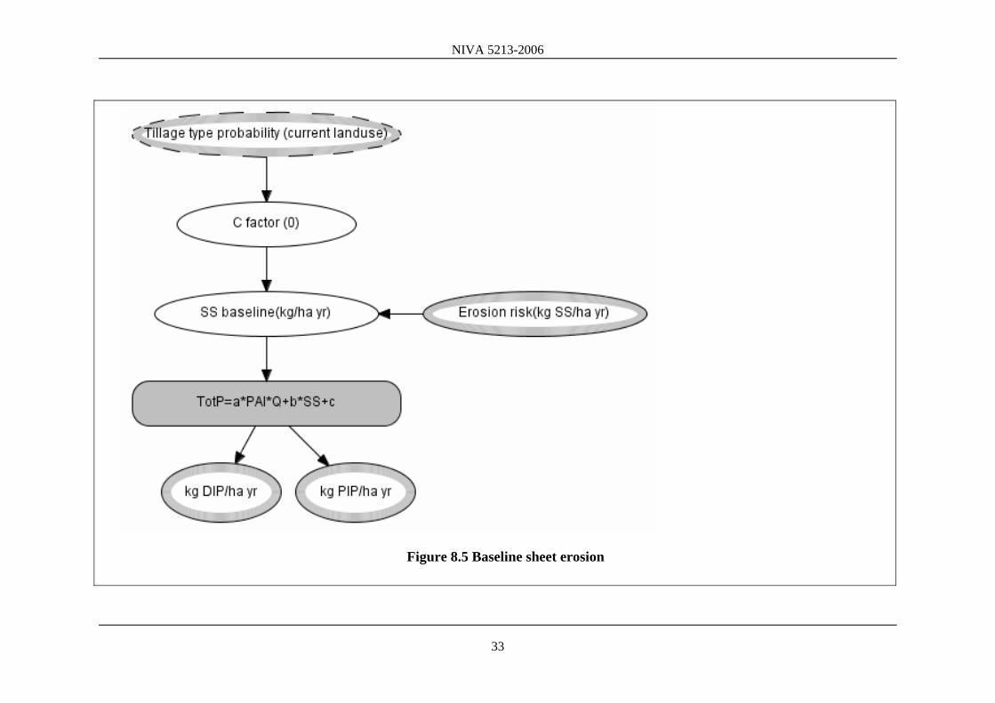
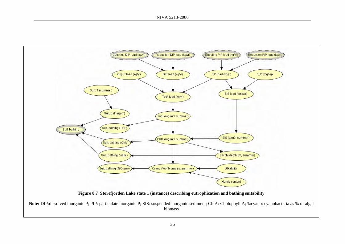
reduction in agriculture and wastewater indicating that the network is an influence diagram which will be used for evaluating the expected utility of sequential decisions to go ahead with wastewater and agricultural measures. In the different instances of Bayesian networks the ‘nodes’ are the ‘chance nodes’ or conditional probability tables (CPT) (ovals), utility nodes (diamonds) expressing the value of outcomes, and decision nodes (rectangles) representing alternative courses of action. Utility nodes are used to calculated expected utility of decisions. Input/output variables linked to the different ‘instances’ are ringed in grey. In figures 8.1-8.8 the underlying “instances” (sub-networks) are illustrated. Figures 8.1-8.4 depict the networks for evaluating cost-effectiveness of tillage measures, vegetation buffer strips, sedimentation dams and individual waste water treatment, respectively. Waste water treatment data and problem structure were taken from Lyche Solheim et al. (2001). Networks on agricultural measures have been revised relative to Barton et al. (2005) based on discussions with experts on run-off (Jordforsk/Bioforsk), and probability distributions reflect a variety of data sources including expert opinion, empirical data and regression model results. Abatement measures’ cost-effectiveness The abatement measures in agriculture have nested ‘instances’ for evaluating “Baseline sheet erosion” (Figure 8.5), which in turn contains an instance for predicting “Tot-P” based on soil Pal, run-off and SS (Figure 8.6). Conditional probabilities predicting Tot-P as a function of soil PAl, run-off and erosion-risk were adapted from a USLE-based regression model in Eggestad, Vagstad and Bechmann (2001), using parameter distributions (mean, st.error) provided by Marianne Bechmann (personal communication). Uncertainty regarding erosion risk in Morsa was modelled as the variability in erosion risk classes for the whole of region Øst17 from the same study (pers. com Eggestad). Run-off was set equal to rainfall for Øst1. No specific data on variation in PAl was used in the model and must be determined as ‘evidence’8 by the user. Changes in C-factors define the effectiveness of changed tillage practices - uncertainty regarding C-factors was obtained from Eggestad (personal communication). Water quality simulation In figure 8.7 the instance describing how eutrophication and bathing suitability state is driven by changes in particulate (PIP) and dissolved (DIP) phosphorous loading. The MyLake model (Saloranta and Andersen, 2004) was run for hydrological and nutrient data for 1995-2000 generating CPTs for relationships between Tot-P-loading – Tot-P-concentrations – chlorophyll a concentrations (Figure 9). The nodes in this instance represent input-output tables of the dynamic eutrophication model MyLake and the cyanobacterial proportion table, as well as a series of water quality criteria indicating bathing suitability. The probability table for cyanobacteria thus has 200 entries: 5 cyanobacteria states x 10 chlorophyll states x 2 alkalinity states x 2 humic states. This instance is central to the whole network and allows a 7 Askim, Eidsberg, Hobøl, Rakkestad, Skiptvet, Spydeberg, Trøgstad 8 ‘evidence’ is a term used in Bayesian networks to denote the fixing of a node to a particular value within its probability distribution, simulating a situation whereby we have evidence of the nodes values with certainty.

NIVA 5213-2006

18

comparison of utility (costs) of measures and utility (benefits) of improvements in bathing suitability. The impact on bathing suitability of reductions in loading are found by the differences in probability of suitable conditions between Storefjord Lake state 0 and state 1 (figure 8.7). Figure 8.7 Storefjorden Lake state (instance) describing eutrophication and bathing suitability The links from chlorophyll a to secchi depth (transparency) and to the proportion of cyanobacteria are defined by conditional probability tables, where the probabilities are calculated as proportions of observations within each combination of states. The data used for parameterising the tables consist of samples Norwegian lakes, all collected and identified by NIVA. The sampling period span from 1972 to 2002, and a large proportion of the samples of the samples were taken during the national eutrophication survey in 1988. Earlier analyses of these data are reported by Lyche Solheim et al. (2004). In order to obtain a dataset that is representative for Lake Vansjø, and at the same time contains enough samples to parameterise the probability tables, we investigated the relationship between chlorophyll a and proportion cyanobacteria for different combinations of geographic ranges and lake types (Figure 10). The best fit (R2 = 0.50) was obtained by data from lowland lakes (<200 m.a.s.l.) of all types in Eastern Norway, analysed with alkalinity and humus levels as covariates (in total 418 samples). The Vansjø lake group alone did not cover the eutrophication gradient well enough, and a wider geographic distribution resulted in more noise. The Swedish and Finnish data used for this initial testing belong to the Lakes database of the EU project REBECCA (www.rbm-toolbox.net/rebecca). The proportion of cyanobacteria is calculated as the biomass of all cyanobacteria except the genus Merismopedia, divided by the total phytoplankton biomass. Proportion of cyanobacteria generally increases with chlorophyll a concentration, but the phytoplankton community may also be affected modified by factors such as alkalinity and humic content (Lyche Solheim et al. 2003b). According to the WDS typology, Lake Vansjø belongs to the low-alkalinity, high-humus lake group. However, the lake chemistry is close to the limit for both typology parameters (4 mg/L Ca and 5 mg/L TOC). We have therefore included two states (high and low) for both of these two parameters, so that the network can cover all four lake groups defined by these parameters. Willingness to pay for bathing suitability From Magnussen et al. (1995) we obtained mean household Willingness to Pay (WTP) for improvements in suitability of water in the Morsa catchment, with watershed population statistics coming from the Norwegian Bureau of Statistics. Figure 8.8 illustrates an instance of how willingness to pay for improvements in bathing suitability are determined through a comparison of the probabilities of suitability in state 0 and state 1. Furthermore, it illustrates that there is uncertainty about benefits determined by uncertain willingness to pay per household, as well as uncertainty regarding the total number of households over which benefit from the improvement are to be aggregated. Figure 8.8 Benefits of bathing suitability changes

NIVA 5213-2006

19

6. Preliminary results

Bayesian belief networks in Hugin can provide a series of generic and problem specific “results” depending on the interests of scientists, stakeholders and managers.

Cost-effectiveness analysis of a programme of measures. In Figure 11, the nodes called “kr/kg TotP: measure” shown previously in Figure 8, have been expanded to examine each measure’s cost-effectiveness. Cost effectiveness is here measured as “kr/kg” of the ‘end-of-field’/end-of-pipe’ for each nutrient abatement measure, i.e. without regard to the eutrophication effect in downstream Storefjorden. We see from the PDFs that the same broad ranking as in Lyche Solheim et al. (2001) cost-effectieness analysis is evident Tillage/ploughing measures are most cost-effective, individual waste water treatment measures are least cost-effective (see Table 1). The difference from the deterministic analysis is that unequivocal ranking of measures is more difficult due to uncertainty both in costs and effects. Cost-benefit analysis of derrogation. Figure 12 illustrates an evaluation of benefits, which can be compared to costs evaluated in Figure 11. Implementing all measures (denoted as “true”/”alternative” in fig.12) still leads to a high probability of WTP for bathing being close to zero, i.e. that no signficant effect on suitability can be observed. In this analysis abatement costs would be deemed “disproportionate” to benefits in the terminology of the EU Water Framework Directive9. The working hypothesis is that cumulative uncertainty in the linked models is too large to be able to demonstrate benefits of the programme of measures. Possible explanations for this lack of observed effect were discussed in the introduction to this report:

• excessively complicated network structure resulting in possible redudancy10 of some nodes.

• information loss due to the discretisation of PDFs in each node • choice of condition probability data underlying PDFs (data correlations, models

simulations, expert judgement) Deductive analysis. What is the change in probability of an environmental objective such as bathing suitability given ‘evidence’ in different parts of the network? Figure 13 illustrates a case where abatement reduction of DIP and PIP is from 30-50% of baseline loads. By how much would such a nutrient abatement effort increase the probability of suitable bathing conditions? The

9 leading to a derrogation from the WFD objective of “good ecological status” 10 Nodes would be called redundant if the model object/instance of which they are part provides the same or less information to a hypothesis variable than does a simple node. In other words, conditioning a node’s pdf on a number of underlying variables does not reduce the coefficient of variation (CV) relative to alternative sources of information on could use to define the pdf unconditionally. An example could be where the instance representing the regression for nutrient run-off TotP=aPAL*Q+bSS+c provides less information (larger CV) than expert judgement of an unconditional pdf for TotP. PAL, Q and SS would be called redundant.

NIVA 5213-2006

20

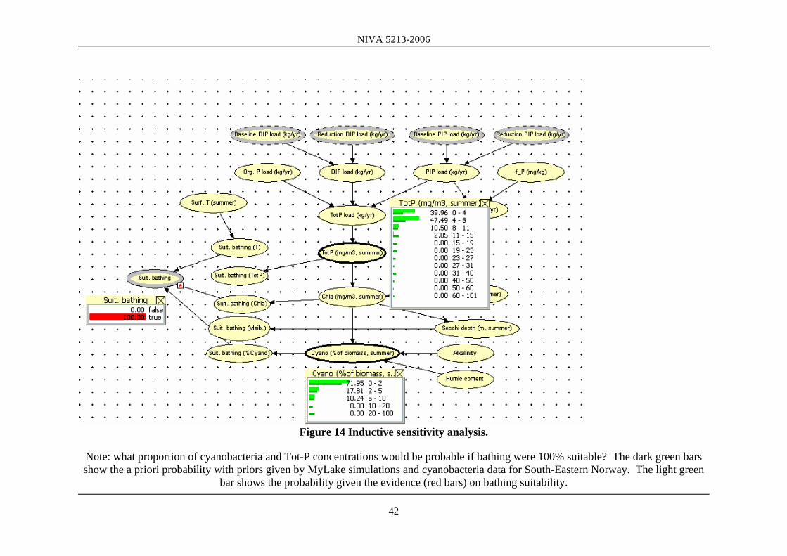
difference in probability is shown to be marginal (but depends on a number of conditioning variables such as bathing temperature). Inductive analysis. What is the change in probability of ‘parent nodes’ (representing causes or input data) given ‘evidence’ we observe for a given ‘child nodes’ (representing objectives of interest)? Figure 14 illustrates the question of what proportion of cyanobacteria and Tot-P concentrations would be probable if bathing were 100% suitable? The analysis shows that significant reductions in Tot-P concentration and cyanobacteria proportion are expected a priori.

Value of information analysis Which variables contribute the most to reduction in uncertainty about a hypothesis variable such as bathing suitability? Figure 15 illustrates this type of analysis using drop down menu functionality in Hugin - an entropy indicator (H) for the ‘hypothesis variable’ “suitability bathing” is given for a situation where we have no observations on the explanatory ‘information variables selected by the user. The information variables are ranked in order of which one contributes the most to reducing this entropy indicator where H()=0 indicates no entropy (i.e. certainty). In the example we see that observations of ChlA give more information than proportion of cyanobacteria - this rhymes with the difference in a priori knowledge seen in the conditional probability tables discussed in Appendix 1. Observing abatement reductions in nutrient loadings gives the least value of information of the variables selected. This analysis can also be conducted associating monetary values to the entropy indicator, in order to compare benefits of additional information with monitoring costs.

NIVA 5213-2006

21

7. REFERENCES Ames, D. P., B. T. Nielson, et al. (2005). "Using Bayesian networks to model watershed

management decisions: an East Canyon Creek case study." Journal of Hydroinformatics 07.04: 267-282.

Barton, D. N., T. Saloranta, et al. (2006). "Using Bayesian network models to incorporate uncertainty in the economic analysis of pollution abatement measures under the water framework directive." Water Science and Techology: Water Supply 5(6): 95-104.

Borsuk M.E., Stow C.A. and Reckhow K.H. (2004). A Bayesian network of eutrophication models for synthesis, prediction, and uncertainty analysis. Ecological Modelling, 173, 219–239.

Bromely, J., N. A. Jackson, O.J. Clymer, A.M. Giacomello, F.V. Jensen (2005). "The use of Hugin to develop Bayesian networks as an aid to integrated water resource planning." Environmental Modelling & Software 20: 231-242.

Eggestad, H. E., N. Vagstad, M. Bechmann (2001). Losses of Nitrogen and Phosphorous from Norwegian Agriculture to the OSPAR problem area, Jordforsk report 99/01.

EU (2000). Council Directive of 23 October 2002. Establishing a framework for community action in the field of water policy (2000/60/EC). Official Journal of the European Communities, L327, 22 December.

Interconsult (2002). Utviklingen i Vannsjø. Konsekvenser for vannforsyningen, MOVAR. Kjærulff, U. B. and A. L. Madsen (2005). Probabilistic Networks - An Introduction to

Bayesian Networks and Influence Diagrams, Departmen of Computer Science, Aalborg University and HUGIN Expert A/S.

Kozlov, A. V. and D. Keller (1997). Nonuniform dynamic discretization in hybrid networks. Thirteenth Conference on Uncertainty in Artificial Intelligence (UAI-97), August 1-3, 1997.

Larsen D.P. and Mercier H.T. (1976). Phosphorous retention capacity of lakes. J. Fish. Res. Board Can. 33, 1742-1750.

Lyche Solheim A., Vagstad N., Kraft, P., Løvstad, Ø, Skoglund, S., Turtumøygard, S., Selvik, J.(2001). Tiltaksanalyse for Morsa. Vannsjø-Hobøl Vassdraget. Sluttrapport, NIVA, Jordforsk, Limnoconsult. NIVA rapport 4377-2001.

Lyche Solheim A., Borgvang S.A., Vagstad N., Barton D., Øygarden L., Turtumøygrad S., Braband Å and Røhr P.K. (2003a). Demonstrasjonsprosjekt for implementering av EUs Vanndirektiv i Vansjø-Hobøl. Fase 2: Skisse til veildere for karakteriseringsoppgavene i 2004, samt forslag til overvåkningsprogram. NIVA rapport 4737-2003, 107 s.

Lyche Solheim, A., Andersen, T., Brettum, P., Erikstad, L., Fjellheim, A., Halvorsen, G., Hesthagen, T., Lindstrøm, E.-A., Mjelde, M., Raddum, G., Saloranta, T., Schartau, A.K., Tjomsland, T., og Walseng, B. 2003b. Foreløpig forslag til system for typifisering av norske ferskvannsforekomster og for beskrivelse av referansetilstand, samt forslag tilreferansenettverk. Oppdragsgivere, SFT, DN og NVE. NIVA-rapport 4634-2003.

Lyche Solheim A., Andersen T., Brettum P., Bækken T., Bongard T., Moy F., Kroglund T., Olsgard F., Rygg B. and Oug E. (2004). BIOKLASS – Klassifisering av økologisk statu i norske vannforekomster: forslag til aktuelle kriterier og foreløpige grenseverdier mellom god og moderat økologisk status for utvalgte elementer og påvirkninger. NIVA Rapport Lnr. 4860.

Magnussen K., Bergland O., Navrud, S. (1995). Overføring av nytte-estimater: status i Norge og utprøving knyttet til vannkvalitet. Del II Utprøving knyttet til vannkvalitet, NIVA.

NIVA 5213-2006

22

Olesen K.G., Lauritzen S.L. and Jensen F.V. (1992). aHugin: A system creating adaptive causal probabilistic networks. In: Proceedings of the Eighth Conference on Uncertainty in Artificial Intelligence (D. Dubois et al., eds), Stanford, California, July 17-19. Morgan Kaufmann, San Mateo, pp. 223-229.

Raiffa H. (1968). Decision Analysis, Introductory Lectures on Choices under Uncertainty. Addison-Wesley, Reading, Massachusetts.

Saloranta T., Andersen T. (2004). MyLake (v.1.1): Technical model documentation and user's guide for version 1.1. NIVA Rapport Snr. 4838.

Skiple Ibrekk A., Barton D.N., Lindholm O., Vagstad N.H., Iversen E. and Berge D. (2004). Systematisk gjennomgang av ulike miljøforbedrende tiltak og forslag til forbedring av metodikken ved tiltaksanalyser i lys av ”Rammedirektivet for vann”. NIVA Rapport Nr. 4777 – 2004

Uusitalo, L. (2006 in press). "Advantages and challenges of Bayesian networks in environmental modelling." in press.

Varis, O. (1997). "Bayesian decision analysis for environmental and resource management." Environm. Modell. Softw. 12: 177-185.

Varis, O. (1998). "A belief network approach to optimisation and paramenter estimation: application to resource and environmental management." Art. Intellig. 101: 135-163.

Varis, O., Kuikka S. (1999). Learning Bayesian decision analysis by doing environmental and natural resources management. Ecological Modelling, 119, 177–195.

Vose D. (1996). Quantitative Risk Analysis. A Guide to Monte Carlo Simulation Modelling. Chichester, John Wiley & Sons.

WATECO (2002). Economics and the Environment. The implementation challenge of the Water Framework Directive. A Guidance Document, WATECO Working Group.

NIVA 5213-2006

23

Table 1. Results of cost-effectiveness analysis of existing abatement plan for Morsa catchment (Lyche Solheim et al., 2001).

Quantified measure Cost/Yr

(1000 kr) Effect (kg red. Tot-P)

Cost/effect

(1000 kr./kg Tot-P) Biofactor b

Effect

(kg red. bio-P)

Cost/Effect

(1000 kr./kg bio-P) Ranking

Agriculture

Plowing practices 297-825 3,300 0.09-0.25 0.2 660 0.45-1.25 1

Vegetation zone 28-56 100-200 0.27 0.2 20-40 1.35 2

Sedimentation dams 730-1,700 1,300-1,700 0.49-1.13 0.2 260-340 2.44-5.67 4

Grassy water courses - - - - - -

Total Agricult. 1,055-2,580 4,700-5,200 930-1,030

Individual wwater 10,431 1,531 6.8 0.7 1,072 9.7 5

Municipal sewage

Red. faulty connections 293-583 301 1.0-1.9 0.6 181 1.6-3.2 3

Red. spillover - 109 - 0.6 65 -

Red. leakage municipal - 104 - 0.6 62 -

Transfer of municipal Wastewater (today) 3500 67 52 0.3 20 175 7

Transfer of municipal wastewater (future) 3500 201 17 0.3 60 58 6

Total wastewater ca. 4000 368 200

Total abatement 15,279-17,094 6,600-7,100 2,220-2,344

Note 1: calculated abatement need was 8,651 Tot-P/yr.

NIVA 5213-2006

24

Figure 1. Achieving “good status” expressed as a likelihood (Skiple Ibrekk et al., 2004).

Figure 2 Conditional probability table

Note: CPT is a ”response surface” representing data correlations, model simulations or expert opinion

NIVA 5213-2006

25

Figure 3. Probability distribution examples.

Source: Barton et al. (2005)

Figure 4. Influence diagrams and Bayesian networks in the context of DPSIR

Note: Prior knowledge: Probability of water quality state S: Pr(S); Probability of nutrient loading pressure P: Pr(P). Posterior: Probability of a state given a pressure: Pr( S | P). Likelihoods: Probability of pressure given a state: Pr (P | S)

NIVA 5213-2006

26

Figure 5 Object-oriented Bayesian network (OOBN) modelling

Note: Hugin Expert can be used to model risk problem structure and uncertainty (model simulations, data-correlations and expert judgement) in an object oriented meta-model. The meta-model describes uncertain processes in the form of CPTs (risk elements) which are organised in Bayesian Networks/Influence Diagrams, which in turn can be organised as objects in a hierarchy. Objects are called “instances” in Hugin and the hierarchical problem structure is called an Object-Oriented Bayesian Network (OOBN)

Figure 6. Methodology and data sources.

NIVA 5213-2006

27

Figure 7. Conceptual illustration of diverse model results to be combined in a benefit-cost analysis of eutrophication abatement

measures Note: response surfaces are depicted as certain. See Appendix 1 for an illustration of response surfaces as conditional probabilities

Source: Barton et al. (2005)

NIVA 5213-2006

28

Figure 8 Aggregated Bayesian network for Morsa catchment problem

Note: grey nodes are ‘instances’ of Bayesian networks describing underlying models and datasets

NIVA 5213-2006

29

Figure 8.1 Tillage practices (agricultural landuse)

NIVA 5213-2006

30

Figure 8.2 Vegetation buffer strips

NIVA 5213-2006

31

Figure 8.3 Sedimentation dams

NIVA 5213-2006

32

Figure8.4 Individual household wastewater treatment plants

NIVA 5213-2006

33

Figure 8.5 Baseline sheet erosion

NIVA 5213-2006

34

Figure 8.6 TotP regression (TotP=aPAl*Q+b*SS+c)

NIVA 5213-2006

35

Figure 8.7 Storefjorden Lake state 1 (instance) describing eutrophication and bathing suitability

Note: DIP:dissolved inorganic P; PIP: particulate inorganic P; SIS: suspended inorganic sediment; ChlA: Cholophyll A; %cyano: cyanobacteria as % of algal

biomass

NIVA 5213-2006

36

Figure 8.8 Benefits of bathing suitability changes

Note: WTP/household=willingness to pay per households as expressed in a contingent valuation household survey. # number of households using lake for bathing

NIVA 5213-2006

37

Figure 9. Structure of MyLake dynamic eutrophication model.

Note: variables in red and blue boxes are parts of the MyLake model that are made explicit in the Bayesian network as

nodes with CPTs.

NIVA 5213-2006

38

0 1 2 3 4 5

0.0

0.2

0.4

0.6

0.8

1.0 n = 84

R2 = 0.11

Pro

porti

on c

yano

bact

eria

Eastern Norway, Vansjø lake group

0 1 2 3 4 50.

00.

20.

40.

60.

81.

0 n = 151

R2 = 0.468

Norway, Vansjø lake group

0 1 2 3 4 5

0.0

0.2

0.4

0.6

0.8

1.0 n = 369

R2 = 0.323

Nordic countries, Vansjø lake group

0 1 2 3 4 5

0.0

0.2

0.4

0.6

0.8

1.0 n = 418

log Chlorophyll a (µg/L)

Pro

porti

on c

yano

bact

eria

Eastern Norway, all lake groups

R2 = 0.501

0 1 2 3 4 5

0.0

0.2

0.4

0.6

0.8

1.0 n = 928

log Chlorophyll a (µg/L)

Norway, all lake groups

R2 = 0.339

0 1 2 3 4 5

0.0

0.2

0.4

0.6

0.8

1.0 n = 1799

log Chlorophyll a (µg/L)

Nordic countries, all lake groups

R2 = 0.343

Figure 10. Analyses of relationship between chlorophyll a and proportion of cyanobacteria for different combinations of geographic region and lake groups. Note: Upper panel: data from the "Vansjø lake group" (low alkalinity, high humic content), indicated as black circles on the map; lower panel: data from all lakes (black and white circles, with alkalinity and humic levels as covariates. Left panel: data from lowland Eastern Norway (indicated by the oval); middle panel: data from all of Norway; right panel: data from Norway, Sweden and Finland. n is number of samples. R2 indicates proportion of variation explained by the regression model (generalised additive model).

NIVA 5213-2006

39

Figur 11 Cost-effectiveness of autumn tillage, buffer strips, sedimentation dams and individual waste water treatment plants

(Hugin Expert analysis window).

Note: Cost- effectiveness ranking is broadly similar to deterministic spreadsheet results illustrated in Table 1, except that ranking of tillage and buffer strips is now more ambiguous.

NIVA 5213-2006

40

Figure 12 Evaluating the uncertain benefits of a programme of measures Note: Setting all measures to “true”/”alternative” still leads to a high probability of WTP for bathing being zero, i.e. that no signficant effect on

suitability can be observed. In this analysis abatement costs are obviously disproportionate.

NIVA 5213-2006

41

Figure 13 Deductive sensitivity analysis. If abatement reduction of DIP and PIP was from 30-50% of baseline loads how much would it increase the probability of suitable bathing

conditions? The dark green bars in “suit.bathing” node show the a priori probability with no priors as to the baseline or reduction in nutrient loading. The light green bar shows the probability given the evidence (red bars) on baseline and abatement reductions. The difference in probability is shown to be marginal (but depends on a number of conditioning variables such as bathing temperature ).

NIVA 5213-2006

42

Figure 14 Inductive sensitivity analysis.

Note: what proportion of cyanobacteria and Tot-P concentrations would be probable if bathing were 100% suitable? The dark green bars show the a priori probability with priors given by MyLake simulations and cyanobacteria data for South-Eastern Norway. The light green

bar shows the probability given the evidence (red bars) on bathing suitability.

NIVA 5213-2006

43

Figure 15 Value of information analysis

Note: The initial entropy of the hypothesis variable “suitability bathing is H(suit. bathing) = 0.38 without any observations on the information variables listed in the window above . The information variables are ranked in order of which contributes the most to reducing

this entropy indicator where H()=0 indicates no entropy (certainty). We see that observations of ChlA give more information than on cyanobacteria this rhymes with the difference in a priori knowledge seen earlier). Observing abatement reductions in nutrient loadings

gives the least value of information of the variables selected. The analysis can also be conducted associating monetary values to the entropy indicator, in order to compare with monitoring costs.

NIVA 5213-2006

44

Appendix 1 – Conditional probability table illustrator

Hugin Expert software makes problem structuring easily accessible to laymen or experts unfamiliar with Bayesian networks, though its graphical user interface (GUI). However, the often large conditional probability tables that lie behind network nodes are not as easy to evaluate intuitively. Hugin Expert provides a bar-illustration (Figure A1) which makes CPTs easier to check if discretisation intervals are uniform. Where discretisation intervals are not uniform it may be more difficult for experts to check whether the data provided has been correctly entered in the CPT. It may also be more difficult to explain to non-experts the nature of the conditional probabilities. Particularly where responses surfaces show thresholds, the non-uniform discretisation/scaling of the CPT may hide this information. Figure A1 - illustration of CPT in Hugin as number observations and bar charts of relative probability mass.

In order to facilitate presentation and itnerpretation of CPT data the EutroBayes project (T. Saloranta) has programmed a ‘CPT-illustrator’ which shows CPTs with axes to scale (normal or logarithmic) and presents probability mass or denisities depending on requirements. At present the CPT illustrator can only deal with simple CPTs of the form P(a | b). CPTs conditioned on a parent node with more than one state, and/or on several parents have to be split into individual tables for every conditioning state. This is illustrated in Figure A2 for the node “ChlA” from the Storefjorden instance (Figure 8.7). The upper panel represents ChlA values given TotP for the lowest and highest conditioning particle sedimentation rates (SIS=1-1.2 g/m3, SIS=3.5-6 g/m3) in the MyLake model. Figure A3 shows the CPTs for % cyanobacteria given ChlA concentrations and four different lake types (humic low/high,

NIVA 5213-2006

45

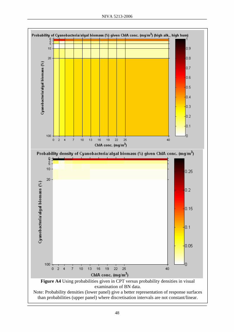
alkaline low/high). A comparison of the conditional probability distributions from the Mylake model (figure A2) and the cyanobacteria proportion data (figure A3) make it immediately clear that there is more uncertainty regarding the latter because a clear response surface is less visible. The above CPTs illustrate probability mass, but can also be misinterpreted. The lower right hand panel of Figure A3 (high alkalinity, high humic lake state) seems to show parallel spikes in the response surface of proportion cyanobacteria to ChlA (proportion cyanobacteria is seemingly high and low for the same values of ChlA). This is an artefact of the discretisation intervals. When probability mass is normalised by the discretisation interval, probability density shows a single (very) weak response surface or gradient of cyanobacteria to ChlA (FigureA4).

NIVA 5213-2006

46

Figure A2 Partial CPTs for node “ChlA (mg/m3)” in Storefjord Lake instance

Note: The figure illustrates the conditional probability table for ChlA conditional on TotP

concentration and selected alternative parameter values for sediment in suspension (SIS=1-1.2, SIS=3.5-6 g/m3)

NIVA 5213-2006

47

Figure A3 CPT for Cyano (% of biomass, summer).

Note: The figure illustrates the conditional probability table for Cyanobacteria given concentrations of ChlA, given different types of alkaline and humic lake classes. Comparison with the previous figure A2 shows the considerably greater uncertainty reflected in

empirical correlations versus model simulated correlations.

NIVA 5213-2006

48

Figure A4 Using probabilities given in CPT versus probability densities in visual

examination of BN data. Note: Probability densities (lower panel) give a better representation of response surfaces

than probabilities (upper panel) where discretisation intervals are not constant/linear.