1. INTRODUCTION

3DM Analyst Mine Mapping Suite is a digital photogrammetric system that is currently being used by mapping, surveying, mining, and engineering companies in Australia, Canada, Indonesia, Japan, Norway, the UK, the US, and Venezuela. It represents the culmination of ten years’ research and development in digital photogrammetry and builds on ADAM Technology’s 20-year history of designing and manufacturing analytical stereoplotters and the associated mapping software.

Although photogrammetry has a well-established reputation for remote measurement and remains a mainstay of the aerial mapping industry, until recently its use was limited to well-trained professionals with good stereo perception and an intimate knowledge of the underlying theory.

With the advent of high quality yet affordable digital cameras, ADAM has developed a system that retains all of the rigor of a state-of-the-art photogrammetric system but with a degree of performance and automation that make it accessible to anybody who can capture an image.

A measure of our success in achieving that goal can be gleaned from the range of tasks that the software is being used for today: geological and geotechnical analysis, resource modeling, end-of-month pickup, stockpile volumes, truck volumes, aerial mapping, road subsidence monitoring (accurate to 1mm),

teeth wear measurement (accurate to 5 microns), and the monitoring of stretch, wear, and corrosion on the chains used to anchor offshore oil and gas platforms — almost all of which are being performed by customers who had no prior experience with photogrammetry.

One of the most popular applications is pit wall mapping for geotechnical analysis. Key reasons for this include:

(i) The ability to capture large areas of pit wall easily and safely simply by photographing them.

(ii) The ability to obtain data from up to 3 km away or from the air when there is no safe access to the area being mapped.

(iii) The ability to identify features that would otherwise not be apparent when working too close to the rock face.

(iv) The speed with which the data can be generated compared to other techniques.

(v) The level of accuracy and detail of the data generated compared to other techniques.

(vi) The fact that acquiring the data has little impact on mining activities.

(vii) The ability to acquire data in a wide range of climactic conditions.

Laser and Photogrammetric Methods for Rock Face Characterization (F. Tonon and J. Kottenstette, eds.)

Using 3DM Analyst Mine Mapping Suite for Rock Face Characterisation

Birch, J. S. ADAM Technology, Perth, Western Australia

Copyright 2006, ARMA, American Rock Mechanics Association This paper was prepared for presentation at the workshop: “Laser and Photogrammetric Methods for Rock Face Characterization” organized by F. Tonon and J. Kottenstette, held in Golden, Colorado, June 17-18, 2006.

This paper was selected for presentation by F. Tonon and J. Kottenstette following review of information contained in an abstract submitted earlier by the author(s). Contents of the paper, as presented, have not been reviewed by F. Tonon and J. Kottenstette, and are subject to correction by the author(s). The material, as presented, does not necessarily reflect any position of USRMS, ARMA, their officers, or members. Electronic reproduction, distribution, or storage of any part of this paper for commercial purposes without the written consent of ARMA is prohibited. Permission to reproduce in print is restricted to an abstract of not more than 300 words; illustrations may not be copied. The abstract must contain conspicuous acknowledgement of where and by whom the paper was presented.

ABSTRACT: One of the most popular uses of 3DM Analyst Mine Mapping Suite is the generation of 3D images for geotechnical analysis. This paper will describe the benefits of using digital photogrammetry for this application as well as some of the common problems that are encountered and how to solve them. It will also discuss the importance of camera calibration and how it is performed, the various options for planning a project, and how to predict the accuracy that will be achieved.

(viii) The fact that the images form a permanent record that can be referred back to in the future for reporting and legal issues.

(ix) The fact that the physical components of the system, namely the computer and the digital camera — which are the only parts that can break down — are relatively cheap, available from many suppliers, and easy to replace.

Using a modern digital camera, a pit wall can be photographed and a detailed Digital Terrain Model (DTM) and 3D image generated in less than ten minutes. Given the distance between any two points in a scene (or between any two camera positions) our software is able to generate correctly-scaled data even without any control points or surveyed camera positions; with at least three known locations — control points and/or camera positions — the data can also be registered in a real-world co-ordinate system, even when it is impossible to place control points in or near the area of interest.

Key features of 3DM Analyst Mine Mapping Suite that make it especially attractive as a digital photogrammetric package include:

(i) The speed of the software — given a pair of 11 megapixel digital images, a user can digitize control points, specify camera stations, determine the absolute orientation, and generate a surface model consisting of 350,000 points in around five minutes on a modern PC. Projects can also be processed in batch mode so users don’t need to wait for the data to be generated.

(ii) The level of automation — the software can usually determine the relative orientation of the cameras fully automatically and generate surface models without operator input.

(iii) The ability of the software to detect problems with the data supplied by the user and advise the user on how to rectify those problems.

(iv) The accuracy of the data provided — customers have achieved accuracies of 5 microns from 150 mm away, 0.7 mm from 20 m away, and 0.1 m from 2.8 km away, using standard consumer digital cameras.

(v) The ability of the software to calibrate almost any modern digital camera.

(vi) The level of support offered by ADAM Technology to ensure customers maximize their benefit from using the software.

Capture Images

Determine camera orientations

Generate DTMs & (optionally) 3D Images

Process DTMs in 3DM Analyst or import3D Images into VULCAN for interpretation

Figure 1. Geotechnical analysis workflow.

Figure 2. Geotechnical analysis of a pit wall in VULCAN.

To illustrate where 3DM Analyst Mine Mapping Suite fits in the food chain, Figure 1 shows the typical workflow for geotechnical analysis, while Figure 2 is a real-life example of a 3D Image generated by 3DM Analyst being analyzed in Maptek’s VULCAN software.

2. PRINCIPLES OF PHOTOGRAMMETRY

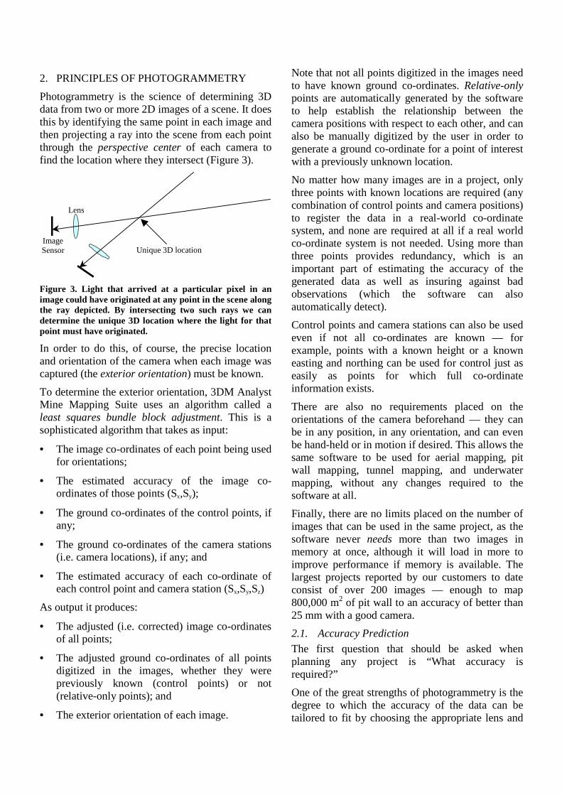
Photogrammetry is the science of determining 3D data from two or more 2D images of a scene. It does this by identifying the same point in each image and then projecting a ray into the scene from each point through the perspective center of each camera to find the location where they intersect (Figure 3).

Image Sensor Unique 3D location

Lens

Figure 3. Light that arrived at a particular pixel in an image could have originated at any point in the scene along the ray depicted. By intersecting two such rays we can determine the unique 3D location where the light for that point must have originated.

In order to do this, of course, the precise location and orientation of the camera when each image was captured (the exterior orientation) must be known.

To determine the exterior orientation, 3DM Analyst Mine Mapping Suite uses an algorithm called a least squares bundle block adjustment. This is a sophisticated algorithm that takes as input:

• The image co-ordinates of each point being used for orientations;

• The estimated accuracy of the image co-ordinates of those points (Sx,Sy);

• The ground co-ordinates of the control points, if any;

• The ground co-ordinates of the camera stations (i.e. camera locations), if any; and

• The estimated accuracy of each co-ordinate of each control point and camera station (Sx,Sy,Sz)

As output it produces:

• The adjusted (i.e. corrected) image co-ordinates of all points;

• The adjusted ground co-ordinates of all points digitized in the images, whether they were previously known (control points) or not (relative-only points); and

• The exterior orientation of each image.

Note that not all points digitized in the images need to have known ground co-ordinates. Relative-only points are automatically generated by the software to help establish the relationship between the camera positions with respect to each other, and can also be manually digitized by the user in order to generate a ground co-ordinate for a point of interest with a previously unknown location.

No matter how many images are in a project, only three points with known locations are required (any combination of control points and camera positions) to register the data in a real-world co-ordinate system, and none are required at all if a real world co-ordinate system is not needed. Using more than three points provides redundancy, which is an important part of estimating the accuracy of the generated data as well as insuring against bad observations (which the software can also automatically detect).

Control points and camera stations can also be used even if not all co-ordinates are known — for example, points with a known height or a known easting and northing can be used for control just as easily as points for which full co-ordinate information exists.

There are also no requirements placed on the orientations of the camera beforehand — they can be in any position, in any orientation, and can even be hand-held or in motion if desired. This allows the same software to be used for aerial mapping, pit wall mapping, tunnel mapping, and underwater mapping, without any changes required to the software at all.

Finally, there are no limits placed on the number of images that can be used in the same project, as the software never needs more than two images in memory at once, although it will load in more to improve performance if memory is available. The largest projects reported by our customers to date consist of over 200 images — enough to map 800,000 m2 of pit wall to an accuracy of better than 25 mm with a good camera.

2.1. Accuracy Prediction

The first question that should be asked when planning any project is “What accuracy is required?”

One of the great strengths of photogrammetry is the degree to which the accuracy of the data can be tailored to fit by choosing the appropriate lens and

working distance. (The accuracy in the direction of view — the depth accuracy — also depends on the ratio between the separation of the cameras and the distance to the pit wall.)

The reason for this is that the accuracy of the generated data depends primarily on the pixel size on the ground — a pixel that is 1 cm × 1 cm on the ground will generally be about ten times as accurate as a pixel that is 10 cm × 10 cm on the ground. (The reason it is not always exactly ten times as accurate is because the final accuracy depends on other factors as well, such as the surveying accuracy of the control points and camera locations.)

The good news is that the size of a pixel on the ground is completely determined by (1) the distance from the camera to the surface in question (distance), and (2) the focal length of the lens being used (f):

sensorground pixelsizef

distancepixelsize = (1)

(All values should be in the same units, e.g. meters.)

For example, a Canon EOS 20D has a pixel size of 6.42 microns. A 28 mm lens from 174 m away will give a ground pixel size of 4 cm × 4 cm. So will a 50 mm lens from 312 m away, a 100 mm lens from 623 m away, a 200 mm lens from 1250 m away, and a 300 mm lens from 1870 m away. (So far, the record for a 3DM Analyst user mapping pit walls for geotechnical analysis is a 3 cm × 3 cm ground pixel size from 2.8 km away using a 300 mm lens with a 1.7 × adapter on a Nikon D2x.) Conversely, given a working distance of 500 m, for example, a user can choose between a pixel size of 11 cm × 11 cm (28 mm lens), 6 cm × 6 cm (50 mm lens), 3 cm × 3 cm (100 mm lens), and so on.

Given the ground pixel size, the actual accuracy that can be expected in the plane parallel to the camera’s image plane (the planimetric accuracy — typically similar to the plane of the pit wall for face mapping) depends on the quality of the calibration, the ability to accurately locate control points in the image, and the accuracy of the control point co-ordinates themselves. The best planimetric accuracy that ADAM Technology has seen so far is a value of 0.05 pixels (0.7 mm in that case) using circular targets located in the image using the software’s automatic centroiding function. A more typical value for planning is 0.3 pixels, with 0.5 pixels being a good conservative value.

Given the expected planimetric accuracy, the separation between the cameras (the base), and the distance from the cameras to the pit wall (distance), the depth accuracy is simply:

cplanimetridepth base

distance δδ = (2)

(Note that this applies to measurements using two images only; observing a point in multiple images captured from different locations allows the depth accuracy to be improved greatly even if the base is small.)

Looking at the formula, it is clear that as the base tends to zero (i.e. the cameras are moved to the same location) the standard error of the depth tends to infinity, as one would expect — when the two camera positions are identical all depth information is lost.

To ensure a good depth accuracy requires a small distance:base ratio, with 1:1 giving the same accuracy in all dimensions. Unfortunately, a large base makes the two different views of the scene look more different, making it difficult for the software (or the user!) to recognize common points. Moving the cameras closer together makes it easier for the software to recognize common points, but reduces the depth accuracy.

Fortunately, the “sweet spot” where the software has little difficulty matching common points while depth accuracy remains good is quite large — we normally recommend distance:base ratios of between 2:1 and 10:1, but the software has been shown to handle a ratio of 1:1 if the surface is reasonably flat (like a pit wall). This gives the user a great deal of flexibility in planning their project to meet both the planimetric and depth accuracy requirements.

2.2. Accuracy Evaluation

The difference between theory and practice, of course, is that in theory there isn’t any.

In practice, however, it’s a good idea to actually check the accuracy that was achieved before using the data — preferably before generating it!

There are several methods of doing this. The most tedious, time-consuming, and accurate method would be to generate the surface models and from them manually measure the locations of the control points to see how close they are to the surveyed locations. The advantage of this is that it not only

measures the accuracy of the orientations but also that of the DTM generation algorithm and the user’s ability to digitize features as well, so we recommend doing this once in a while.

A much faster and easier method is to simply read the post-orientation report from the software.

Before performing an orientation, the user specifies how accurate they expect the image co-ordinates to be. (For a calibrated camera this should generally be in the range of 0.1 to 0.2 pixels.) They also specify how accurate they expect the control points to be.

The software will take both of these into account when it performs the bundle adjustment and the first number that the user should check is the overall Sigma reported by the software — a value larger than 1 indicates that the data is not as accurate as they claimed it was going to be (indicating a potential problem), and a value smaller than 1 indicates that it is more accurate than expected (suggesting they may have been overly pessimistic on their image co-ordinate sigmas or control point sigmas, or perhaps they don’t have enough redundancy.) A value close to 1 is a good sign.

The next thing to look at is the residuals of the control points. Provided there is enough redundancy, this should give a good indication of how accurate the orientations are.

Finally, the user should look at the residuals of each individual control point and check that none of them are anomalous — an unusually large figure suggests a problem with the control point that warrants further investigation. (In our experience, the answer often turns out to be bad survey data; the biggest error in a control point’s location we have seen so far was 2 km, but smaller errors are not uncommon.) The software can automatically check control points and report any that are suspicious.

Photogrammetric best practice dictates that the user should also consider withholding the co-ordinates of a set of control points to allow them to be used as check points. These should be digitized in the usual manner and the software used to derive their locations, and these locations then checked against the surveyed locations. If all is well, their residuals should be similar to the residuals of the other control points that were used to control the orientations. (If they are much larger then there may be insufficient redundancy and the software is “over-fitting” the orientations to the limited control

it has.) A simple way to do this is to simply give them very large sigmas (e.g. 1000 m or more) so they have no bearing on the bundle adjustment solution — this has the advantage of getting the software to calculate the residuals automatically.

It is worth noting that the accuracy of the control points (determined by looking at their residuals) will tend to be higher than the accuracy of other features, particularly those that are measured using the generated surface model.

This is partly because control points tend to be easy to identify; in the best case, circular targets are used and the software can locate the center of those very accurately — often better than 0.1 pixels, much more accurately than a human can identify a point. Even when manually measured, the user will tend to take more care trying to locate the point accurately than when digitizing normal features.

The other reason, however, is that data derived from the surface model is also subject both to the matching accuracy of the software when generating the points on the surface (typically about 0.3 pixels), and the sampling error caused by the discretization of the surface itself (the software will only generate points about every 8 pixels by default, although this can be adjusted by the user down to every 4 pixels if desired) in addition to the accuracy of the orientations themselves.

The matching accuracy can also be degraded by noise in the images, which is why ADAM always recommends using ISO 100 for the image sensor sensitivity.

For this reason, it is still wise to occasionally check control point locations by hand using the DTM as recommended at the beginning of this section.

(Note that operators using the Stereo View are not subject to the accuracy of the DTM; manual observations in this view can often approach the accuracy of the orientations.)

3. IMAGE CAPTURING TECHNIQUES

The flexibility of the software with regard to camera orientations that was mentioned previously allows a great deal of latitude in the design of image capturing procedures.

The three most common procedures that we recommend to our customers are convergent images (for individual models), strips (for large projects

where the camera cannot be moved very far from the pit wall), and image fans (where the camera can be moved further away).

In each case, the primary goal is to find the optimum balance between conflicting aims:

(i) To minimise the time and risk associated with capturing images.

(ii) To maximise the robustness and accuracy of the resulting data.

3.1. Independent, Convergent Models

Overlap between models

Figure 4. Independent, convergent models.

The key characteristic of this method is that close to 100% of each image is used in a single model, and if multiple models are required to cover the pit wall there is very little overlap between them. (In practice it would be wise to plan for a 10–20% overlap between models to ensure there are no gaps in the generated DTMs.)

The downside of this method is that each model needs to be fully controlled, and so the surveying requirements are more onerous. (There is some scope for passing control information between models by taking advantage of the overlap between them (see Figure 4), but the accuracy will be worse than if the model was controlled unless the overlap is 30% or more.)

This method is most desirable when only a single model is required.

Other advantages of this technique are:

(i) There is a great deal of flexibility in the distance between the camera stations. The distance:base ratio can be freely chosen between about 2:1 and about 10:1, with the choice being largely determined by the desired depth accuracy of the model and convenient shooting locations.

(ii) This method can be used with cameras of any focal length operating over any distance.

3.2. Strip of Models

Figure 5. Strip of models.

In this method, a series of parallel images with large overlap (typically 60%) are captured.

The key advantage of this technique is that the large degree of overlap between images allows orientation information to be reliably and accurately passed between models, drastically reducing the number of control points required for a given job without sacrificing accuracy.

Apart from being the normal method used with aerial photography, this method is best used when mapping a long stretch of pit wall from a short distance and a short focal length lens (e.g. 28 mm). The Object Distance spreadsheet supplied with 3DM Analyst Mine Mapping Suite can calculate exactly how far apart the camera stations need to be to ensure the entire wall is captured optimally.

During a trial conducted by BMA Coal in 2004 we were able to demonstrate that this technique could be used to control a project consisting of 36 images (mapping 700 m of pit wall) to better than 6 cm using just one control point in addition to the surveyed camera locations, and better than 4 cm using nine control points. BMA Coal now routinely uses one control point for every five images and reports an accuracy of 2 cm on average.

One drawback to using this technique is that the lens focal length determines the distance:base ratio necessary to ensure adjacent images overlap correctly, reducing camera position flexibility. It also makes it less desirable for longer focal length lenses because the distance:base ratio becomes larger, reducing depth accuracy.

3.3. Image Fans

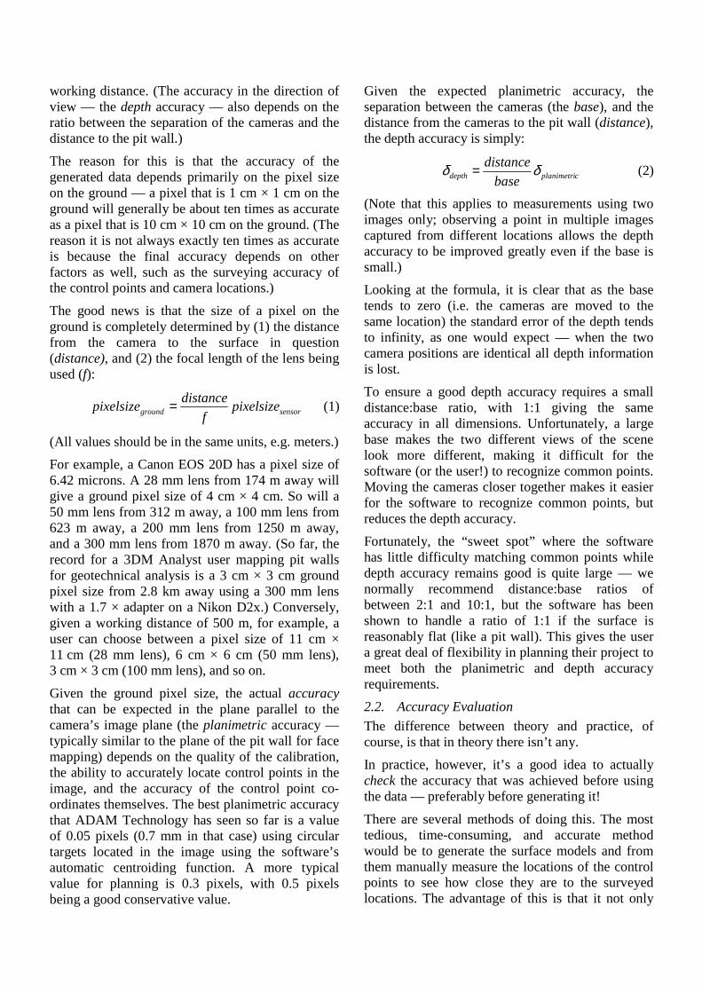
Fortunately, in the cases where long focal lengths are desirable — namely, when the distance to the pit wall is large — the best technique overall becomes available: Image fans (Figure 6).

First model Second model

Figure 6. Image fans.

Image fans are similar to independent, convergent models, except that a series of images are captured from each camera location. Ideally, the images should be captured with a small overlap (at least 10%) to reduce the chance of gaps in the models, and provide the option of sharing orientation information so each model does not necessarily need to be individually controlled.

A key advantage that image fans have over the independent, convergent models is that because multiple images were captured from each location there are far fewer unknowns to be determined by the bundle adjustment. This improves the strength of the solution, makes the bundle adjustment run

faster, and reduces the minimum number of control points required to find a solution down to one for the entire image fan if both camera locations are known.

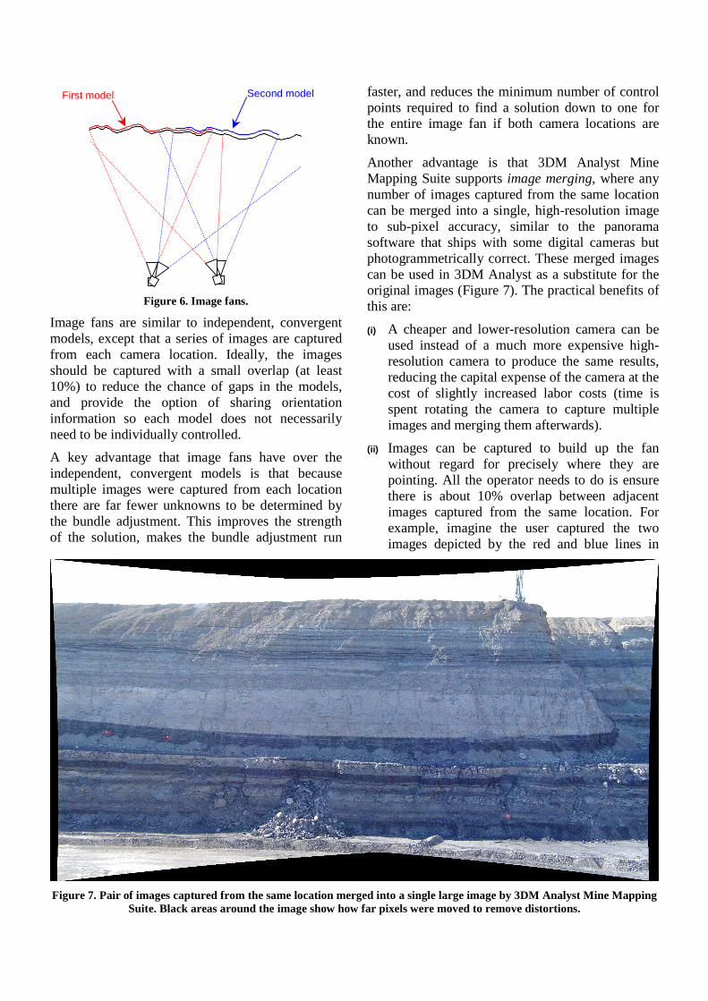
Another advantage is that 3DM Analyst Mine Mapping Suite supports image merging, where any number of images captured from the same location can be merged into a single, high-resolution image to sub-pixel accuracy, similar to the panorama software that ships with some digital cameras but photogrammetrically correct. These merged images can be used in 3DM Analyst as a substitute for the original images (Figure 7). The practical benefits of this are:

(i) A cheaper and lower-resolution camera can be used instead of a much more expensive high-resolution camera to produce the same results, reducing the capital expense of the camera at the cost of slightly increased labor costs (time is spent rotating the camera to capture multiple images and merging them afterwards).

(ii) Images can be captured to build up the fan without regard for precisely where they are pointing. All the operator needs to do is ensure there is about 10% overlap between adjacent images captured from the same location. For example, imagine the user captured the two images depicted by the red and blue lines in

Figure 7. Pair of images captured from the same location merged into a single large image by 3DM Analyst Mine Mapping

Suite. Black areas around the image show how far pixels were moved to remove distortions.

Figure 6 from the left camera station and then moved to the right camera location to capture the corresponding images from there. Normally they would need to ensure that the image of the first model area captured from the second location lined up with the image of the first model area captured from the first location (red lines) so that a convergent model could be formed. Using image merging means that they just need to ensure that the images captured from each location cover the entire area of interest, and later a single, merged image will be created.

The only drawback with this technique is that the merged images can become very large if many images are merged together — the comfortable limit for 3DM Analyst on a PC with 2 GB of RAM is about 65 megapixels. (There is another version of the software, 3DM Analyst Professional, which can handle images in excess of 250 megapixels. This is normally used by mapping companies with scanned large format aerial images.)

To alleviate that, 3DM Analyst Mine Mapping Suite allows the user to tile a merged image to create images that can be processed more comfortably; this is still an advantage over using the original images because the benefits of not having to line images up in the field are retained, and the user is free to choose an image size larger than the native image size of their camera.

Image fans are ideal when longer focal length lenses are used over large distances. Customers have used image fans to capture a 1 km stretch of pit wall with a 4 cm ground pixel size from just two locations on the opposite pit wall, 1 km away.

Apart from the fact that multiple images are captured from each camera location rather than a single, low-resolution image, there really isn’t any conceptual difference between image fans and independent, convergent models, so all of the other attributes of the latter apply to this method as well.

3.4. Combinations

Apart from directly supporting image fans by optionally using a single camera location for multiple images, 3DM Analyst Mine Mapping Suite is completely agnostic when it comes to the method used to capture the images.

One advantage of this is that the user is free to use any combination of techniques they wish in the

same project without any limitations. For example, if the pit wall was too high to be photographed in sufficient detail in a single image, the user might opt to use a strip of images but from each camera location capture two or more images vertically to create a mini-fan.

Alternatively, if the middle two camera positions in Figure 4 were co-located, then image fanning could be used to create a single, wider merged image at each location, with the merged images conceptually forming a strip of images.

The user could also use one method for one section of the wall and a different method for another section if that was more appropriate.

3.5. Control

As mentioned previously, to form an absolute orientation requires at least three known locations — either control points or camera stations.

One of the advantages of surveying camera stations is that the point in question must be safe for the surveyor to access — the image was captured from there, after all. The disadvantage is that the point is further away from the area of interest, which magnifies the surveying error.

Photogrammetric best practice is to bracket the area of interest with control points — the accuracy of the data will be maximized within the region surrounded by control. Going outside this region requires extrapolation, magnifying error.

Sometimes it is not possible to place control near the region being mapped — for example, when mapping a pit wall failure. The most accurate way to map areas like this is to place control a safe distance away on either side (and/or in the background) and capture overlapping images from one controlled area to the other, crossing over the area to be mapped in the process.

Another alternative is to place control points in the foreground, far enough away from the wall to be safe, but not so close to the camera that the surveying error is magnified beyond the accuracy required at the pit wall.

Former images of an area that were previously controlled can also be incorporated into a project to control it — even if the control points used in the former images have been subsequently removed.

3.6. Effort

The amount of effort that should be spent in planning and placing and surveying control should be related to the cost of recapturing images if required and the ability to do so.

Some of our customers use our software to make accurate and detailed models of subsea structures on gas and oil platforms. The daily cost of capturing the images required for that task can be $250,000 per day. Clearly, in their case, they never want to have to go back and capture the images again.

Aerial photography, too, is expensive, often costing around $25,000 to photograph a single mine. It makes sense to plan carefully, place additional control points, and capture additional images, to reduce the chance of having to do the flight again.

Capturing a pit wall, however, is generally a lot less expensive and time-consuming. Except in cases where it will be impossible to capture the pit wall again, it may make more sense to build in less redundancy and occasionally have to re-do the field work than to survey large numbers of control points and go to great lengths to ensure the photography is perfect.

4. GENERATING DATA

Once the camera orientations have been determined, the next step is to identify common points in stereo image pairs in order to project rays into the scene and determine their 3D locations.

In 3DM Analyst this is fairly straightforward — simply clicking on the “GO” button will generate a DTM that can then be viewed in 3D with texture draped over it for analysis, or in stereo with the appropriate viewing hardware.

The time taken to generate the data depends on the size of the images, but between two and five minutes is common. For large projects this can be batch-processed in the DTM Generator, which can process any number of jobs without user intervention, e.g. overnight.

Both 3DM Analyst and DTM Generator can also automatically create 3D Images suitable for use in VULCAN, Surpac, and other software supporting that file format, and 3DM Analyst can also export the DTM in DXF format as points, triangles, or both.

3DM Analyst can also create contours and cross-sections, and calculate volumes — both to a datum and as a difference between two DTMs. It can also merge DTMs together.

Another useful tool is 3DM Ortho Mosaic — an optional extra package that can be used to create seamless mosaics of orthorectified DTMs projected onto any plane.

4.1. Mapping

Due to its mapping heritage, 3DM Analyst features a full complement of mapping tools. It allows up to 160,000 user-defined feature types to be specified in a hierarchy of four levels with 20 feature types per level (Figure 8).

Figure 8. Feature defintions.

Each feature type can be assigned a DXF layer name for importing from and exporting to DXF. Features can be points or lines, among others, and line features can be captured in point-to-point mode, continuous mode (points are added to the line continuously as the floating mark is moved, recording every movement the operator makes), two different arc modes (for curbs, etc.), circle mode, and smooth mode (like point-to-point mode except the points are connected by smooth arcs). The user can switch between modes at any time while digitising a line.

Line features can also affect the DTM:

• Breaklines allow the user to specify that triangles should not cross a certain feature;

• Areas allow the user to specify where DTM points should be automatically generated;

• Holes allow the user to specify where DTM points should not be generated, leaving a hole in the DTM; and

• Flats allow the user to specify that there should be no points within an area but the area itself should remain part of the surface (good for buildings, allowing contours to be generated through buildings as if they weren't there).

Areas, holes, and flats can be nested and the system will honour them all (e.g. the user could specify a hole or a flat line feature around a lake, but an area line feature around an island within the lake).

Lines can also be automatically squared (the software will make nearly parallel lines parallel and nearly perpendicular lines perpendicular if it can do so without moving any point by more than the amount you have specified in the job's accuracy setting — good for digitising buildings) and closed. Dip and dip direction can also be reported if desired for selected feature types and exported for use in other software, like Dips.

Data can be digitised in full colour stereo using either a StereoGraphics’ Z-Screen with polarising glasses or LCD shutter glasses, or in anaglyph mode. It can also be digitised in the 3D View directly onto the DTM, or in the Images View in Single Image Digitising mode (where the software automatically locates the corresponding point in the other image, first by using the DTM then fine-tuning it by performing image matching).

For serious mapping the software also supports ADAM’s full range of handwheels, footdisks, and footswitches as well.

5. CAMERA CALIBRATION

Photogrammetry has traditionally been used with metric cameras — cameras that are designed to resemble the “ideal” camera as much as possible and require very little calibration. Large format film cameras, for example, often have such small lens distortions that verifying the calibrations are being applied correctly can sometimes be a challenge!

In contrast, a compact digital camera or digital SLR with a short focal length lens can easily have lens distortions in the range of 50 to 100 pixels (Figure 9).

Figure 9. Colour-coded lens distortions of a 28mm lens.

Using 3DM Analyst Mine Mapping Suite these cameras can usually be calibrated to an accuracy of between 0.1 and 0.2 pixels using a total of eleven parameters:

(i) Focal length (C): The perpendicular distance from the image sensor to the perspective center of the lens.

(ii) Principal Point Offset (Xp, Yp): The offset from the center of the sensor to the point on the sensor where the direct axial ray passing through the perspective center of the lens intersects the sensor.

(iii) Radial Distortion (K1, K2, K3 & K4): The co-efficients of a polynomial equation describing the distortion radially from the principal point. (Generally only very short focal length lenses need all four terms.)

(iv) Decentering Distortion (P1 & P2): All elements in a lens system should ideally be aligned at the time of manufacture. Any displacement or rotation of a lens element from perfect alignment will cause geometric displacement of images.

(v) Scaling Factors (B1 & B2): Pixel scaling factors that can compensate for any difference in pixel width and height (B1) and non-perpendicularity of the horizontal and vertical axes of the sensor (B2).

Not all lenses require all parameters to correctly characterize their distortions; if this is the case, the affected parameters will be strongly correlated and 3DM Analyst Mine Mapping Suite will identify this during calibration, giving the user the option of disabling one or more of the parameters. We

strongly recommend that the user do this — the aim is to use the smallest set of parameters possible because this will maximize the accuracy of those parameters and avoid “over fitting” the data.

5.1. Camera Restrictions

3DM Analyst Mine Mapping Suite is capable of calibrating virtually any digital camera.

Whether the calibration is generally useful, however, depends on the ability of the user to reproduce the same optical settings on that camera.

On a zoom lens, for example, by far the biggest factor that affects the validity of the calibration is the zoom setting itself. If the zoom setting cannot be reproduced reliably, then the calibration may not be valid. For this reason, we generally discourage the use of zoom lenses: the only two zoom settings that can be reliably reproduced are the minimum and maximum zoom settings, which means a zoom lens is only equivalent to two prime lenses. Since a zoom lens of comparable quality to a prime lens will cost a lot more than two primes (and, generally, it isn’t possible to obtain a zoom lens of comparable quality anyway) then it is better simply to have a set of calibrated prime lenses available to suit the desired working ranges and ground pixel sizes than to try to reduce the number of lenses required by using a zoom.

Of course, compact digital cameras are generally equipped with zoom lenses, so there may not be much choice in the issue. This is one of the reasons why digital SLRs are preferable to compact digitals. (The other main reason is that digital SLRs will have a higher optical resolution and lower noise at a given pixel count than a compact digital.)

Assuming the zoom is constant, the next largest factor that affects the validity of a calibration is the focus setting of the lens. For most outdoor work the traditional approach has been to focus the lens at infinity and tape it up so it can’t move. Whether this is practical or not depends on the range of distances that will be encountered, the aperture size that can be used, and the focal length of the lens.

For example, with a 28 mm lens set to an aperture of f/8 and focused at infinity, everything from about 9 m away should be very sharp.

With a 100 mm lens on f/8 focused at infinity, however, points closer than about 100 m away will start to get blurry.

If a larger aperture is required — for example, to let in more light so a faster shutter speed can be used (e.g. because the camera is being used for aerial photography) or because there isn’t much light to begin with (e.g. underwater or in a tunnel) — then the range of distances that remain acceptably sharp can drop dramatically.

One option is to adjust the focus for the job in question and perform an on-line calibration just for that job (see the next section). However, it is still very important that the user remembers to keep track of the focus setting used for each image to avoid accidentally trying to calibrate a set of images where multiple focus settings were used. (The symptom the user will observe in this case is an inability to bring the calibration accuracy down to the 0.1–0.2 pixel range mentioned previously.)

Another is to simply create calibrations at a range of focus distances and use one that fits best, especially for jobs where the accuracy of the calibration is generally far higher than the accuracy required for the job and so a small bit of calibration error doesn’t really matter.

Another factor that affects the calibration’s validity is the aperture. Changing the aperture has a small scaling effect — a few pixels at worst — and so we recommend to our customers to use a different calibration for each aperture setting if accuracy is absolutely critical. Fortunately, if camera stations are not being used, a small scaling effect is one of the easiest calibration errors for the exterior orientation to compensate for, because the exterior orientation can move the camera slightly closer or further away from the scene to compensate for the calibration error, retaining accuracy in the area of interest.

5.2. On-line Calibration

Although calibrations are normally performed using images that have been carefully planned and captured for that purpose, 3DM Analyst Mine Mapping Suite can actually derive a calibration from the same images that are being used for the pit wall mapping project. If something has changed optically in the camera (e.g. the focus), not only can this be detected but an ad-hoc calibration performed so that the new images can still be used. With enough images, it is even possible to perform a calibration without any control points or surveyed camera positions at all.

The process of performing a calibration (or interior orientation) in 3DM Analyst Mine Mapping Suite is exactly the same as determining the exterior orientation. In fact, the same routines are used internally for both — the only difference is that the interior orientation parameters are automatically fixed when the exterior orientation alone is desired.

In addition to deriving the interior orientation parameters, the software is also capable of analyzing the parameters and generating a report that indicates if any of the parameters are correlated (which affects how reliable the derived parameters are) and how accurately it thinks each parameter has been determined, which allows the user to judge the quality of the calibration.

The software also allows the user to easily compare two calibrations visually.

Although performing a calibration is fairly straightforward, it would be nice if we could simply calibrate each type of camera and lens that our customers were likely to use and supply a generic calibration for them. Unfortunately, comparing the calibrations of identical model lenses and cameras, we have found that this is not possible.

In one trial, for example, one of our customers calibrated two Nikon D2x cameras with the same model 60mm lenses and found that the difference between the calibrations was almost as large as the difference between each calibration and no calibration at all. (This should not be completely surprising — the calibration accuracies that the software achieves amount to less than a micron on a digital SLR; the manufacturers of digital cameras certainly have manufacturing tolerances in the placement of the image sensor or lens elements much greater than that!)

As a consequence we always recommend to each customer that they calibrate each camera + lens combination separately and we normally calibrate their camera and lenses for them during training.

6. PITFALLS

Although photogrammetry has many advantages as mentioned earlier, things can go wrong and it is important that users not only be aware of the problems that can arise, but also know how to deal with them once they have occurred and, ideally, how to avoid them in the first place.

6.1. Bad Imagery

Bad imagery includes both images that actually have something wrong with them (blurry, over- or under-exposed, optically different from the calibration, etc.) and perfectly good images that simply fail to capture the entire area being mapped.

The first problem can be addressed by having good procedures. Ensuring the calibration always matches the camera/lens combination, for example, can be as easy as using a digital SLR with prime lenses and taping the focus ring. If that is not possible or desirable, the problem can be avoided by capturing additional images so an ad-hoc calibration can be performed on a project-by-project basis. (As long as the camera hasn’t changed since the images were captured, this can even be done after the event.)

Motion blur can be fixed either by ensuring the shutter speed is high enough or by using a tripod and possibly a remote shutter release. Aperture priority mode will ensure that the images are not over- or under-exposed, and the camera will show what shutter speed is required for the shot allowing a decision to be made about how to capture it. Using a tripod by default means the photographer doesn’t need to worry about that at all.

To avoid the problem of failing to completely capture the area that needs to be mapped requires careful planning. ADAM Technology supply a spreadsheet that can be used to calculate the number of images that will be required to capture an area with a given camera and lens combination, calculate the required distance from the wall to the camera stations, and determine how far apart the camera stations need to be in order to achieve the desired distance:base ratios.

Using image merging also greatly reduces the risk of areas not being captured in at least two images — when capturing the images from each camera station, the photographer can overlap them as much as they like because excessive overlap won’t affect the size of the final merged image (and hence processing time). Using a great deal of overlap is therefore encouraged, minimizing the risk of gaps.

When capturing image strips, especially from the air, ADAM encourages customers to capture images at least twice as frequently as required — the cost of capturing an image with a digital camera is essentially zero, and having a substitute image

nearby can sometimes be very useful, as customers who have flown through small clouds at the wrong time can attest.

6.2. Bad Observations

There are two types of observational errors that users will encounter:

(i) Bad control point or camera station co-ordinates used for an absolute orientation, usually supplied by another party.

(ii) Incorrectly identified control points or relative-only points observed by the user of the software or by the software itself.

To address the first problem requires redundancy — if there are only three known locations in the whole project then the software cannot tell if they are wrong. However, if there are more than three, the software has very robust and sophisticated mechanisms that can detect bad control data.

One customer’s project featured over 40 images captured from four camera stations, mapping the pit wall of an iron ore mine from 850 m away. The photography had initially been captured for use in another package that processed each model individually and therefore needed a control point for each pair of images, so there were more than 20 control points placed around the bottom of the pit wall.

The customer found, however, that although the generated 3D images lined up well at the bottom of the pit wall where the control points were, there was a 20 m discrepancy at the top of the wall between the 3D images generated by images captured from the first two camera stations and those generated by images captured from the second two.

3DM Analyst Mine Mapping Suite detected that the problem was with two of the camera stations, and predicted that they should have been over 100 m higher than the survey data indicated.

Checking the original survey data indicated that the customer had actually copied the survey data incorrectly, and that our software had predicted the correct location of those two cameras to within 0.5 meters — at a range of 850 m from the pit wall.

Another customer working on an aerial mapping project had the locations of 15 control points supplied by their surveyor. Our software was able to immediately identify that three of them were wrong

— including the one with the 2 km error mentioned earlier. (The surveyor had transposed some digits.)

With customers experiencing an error rate of up to 1 in 5 with the supplied survey data, it is obviously essential that they be able to verify that it is correct. One of the strengths of our software is that it is able to do just that. (There is a long-standing antipathy between surveyors and photogrammetrists; one of the reasons for that is the ability of photogrammetrists to detect when surveyors provide incorrect data!)

The second problem manifests itself in a variety of ways: we have seen one case where two control points were close to each other on a pit wall, and the customer had labeled one of them with a particular ID in one image but used the same ID for the other one in the other image; more commonly the customer simply labels a control point with the wrong ID. In either case the software will detect that the derived 3D co-ordinate for the control point is inconsistent with the supplied survey data. (One good idea is to actually paint the number of the control point on the wall next to it so it can be seen in the images!)

The other problem is bad relative-only points — either digitized manually by the user or generated automatically by the software. Fortunately, when generating relative-only points automatically, the software tends to find between 100 and 200 points (manually digitizing six to nine points was common in the days before automation) and so bad points are relatively easy to detect due to their large residuals. (In fact, the software actually includes a menu item “Edit | Remove Bad Relative-only Points” to identify and remove these points automatically.)

6.3. DTM Generation

Most of the earlier problems manifest themselves when the user attempts to determine the camera orientations. Once that has been done, the next step is to generate the DTMs. Fortunately, if the orientations are successful, there aren’t many things that can go wrong at this point.

One of the things that can go wrong is the generation of “bad points”. These fall into two categories:

(i) Points that the software has incorrectly identified as belonging to the same point in the scene.

(ii) Points that the software has correctly identified as belonging to the same point, but that point is undesirable for some reason. (This is more common in aerial photography — examples include points on vehicles that have moved between images, or points on the tops of trees or buildings where the user is trying to model the ground’s surface.)

The software has two ways of dealing with points of the first type. Firstly, there is a “matching tolerance” setting that the user can use to specify how similar two points must be before they should be considered a match. If many bad points are being generated, the user should consider raising this setting to make it harder to match. (The default setting generally doesn’t create many bad points — the problem usually occurs when the user has lowered the tolerance because they are getting insufficient coverage, e.g. because of very noisy images making matching difficult.) Secondly, bad points of this type generally have 3D co-ordinates that differ markedly from their neighbors, resulting in “spikes”. The software takes advantage of this fact to identify bad points and weed them out. The user can also manually perform a “spike removal” operation with a user-defined level of aggressiveness (i.e. how “spiky” a point must be before it is removed).

Points of the second type are more difficult to deal with (unless the point is on a moving vehicle and it moved far enough that it results in a spike — they can be filtered out in the same way as mismatched points). There are various methods, but unfortunately it is very difficult to explain to the software that you only want points on the ground and not on man-made objects. (Fortunately this problem does not occur much when mapping pit walls!)

Another problem that can occur is that the software simply doesn’t find many points at all. One reason could be an excessive distance:base ratio; another could be excessive noise in the images. Both of these should be avoidable with proper planning. Lowering the matching tolerance is a good first step, keeping an eye out for incorrectly-matched points. Using the Stereo View and digitizing the data by hand is sometimes a last resort, although if the problem is excessive convergence (due to a large base) then it might be difficult for a human to visualize the scene as well.

The final problem that can occur is that coverage of the area being mapped is incomplete, which is a symptom of bad planning.

7. EXAMPLE

Ekati Diamond Mine, situated 200km south of the Arctic Circle, is BHP Billiton's only diamond mine. The extreme weather conditions make field work challenging and highlight the importance of safe data collection techniques.

Using a Nikon D1x with a 135 mm lens from 680 m away on the opposite side of the pit, our customer captured a 500 m x 250 m section of pit wall, representing about 1/3rd of the pit, from just two locations (Figure 10).

Figure 10. Mapping a pit wall.

By mounting the camera on a tripod and panning it up and down to create image fans the pit wall was captured at a ground pixel size of 3 cm x 3 cm (for a detailed structural analysis) within a few minutes. Seven permanent ground control points placed around the outside rim of the pit were used in addition to the surveyed camera stations to provide data accurate to 0.1 m all the way down to the pit floor without any need to place control points there.

Merging the images removed the need to carefully align the images captured from the right camera station with the corresponding images captured from the left camera station, simplifying the field work and reducing the time required (Figure 11).

DTMs and 3D Images were generated in batch mode and imported into VULCAN for geotechnical analysis (Figure 2).

Figure 11. 24 megapixel merged image of a pit wall at Ekati.

8. CONCLUSION

After decades of being limited to aerial mapping and other esoteric applications, photogrammetry is rapidly expanding into new markets as people become increasingly aware of the advancements that digital cameras and faster computers have made possible.

Building on 20 years of experience in the photogrammetric industry, ADAM Technology has developed a tool that sets new standards in automation, user-friendliness, and performance.

3DM Analyst Mine Mapping Suite has proven itself to be a valuable tool for many applications, with one of the fastest growing areas being detailed face mapping. With a level of detail, accuracy, range, and price that is difficult to match using any other technology, ADAM is convinced that the use of 3DM Analyst for face mapping will continue grow rapidly in the future.