user’s manual of flow*
TRANSCRIPT

User’s Manual of Flow*Version 2.0.0
Xin Chen
University of Colorado, Boulder
1 Introduction
Flow* is a tool for safety verification of hybrid systems. Given a real-valued interval∆, a natural number m, and a hybrid system A which is modeled by a hybrid automaton,the tool computes a finite set of Taylor models containing any state of A which is reachablein the time interval ∆ via at most m jumps.
Since the reachability problem, or even the bounded reachability problem on hybridautomata is undecidable [1], we are not able to compute a reachable set exactly in general.Therefore, to prove a safety property Φ on a given hybrid automaton, Flow* tries tocompute an over-approximation of the reachable set which does not violate Φ.
The structure of Flow* 2.0.0 is shown in Figure 1. The tool mainly consists oftwo modules, the computational library and the higher-level algorithms. The formerone contains an interval as well as a Taylor Model (TM) library. In the latter one,the techniques such as integrating TM flowpipes, computing flowpipe/guard intersectionsthat are used in the reachability analysis are implemented. The current version of Flow*supports the hybrid automata such that
- the continuous dynamics in a mode is defined by an Ordinary Differential Equation(ODE) which is allowed to have bounded time-varying uncertainties;
- a jump guard or mode invariant can be defined by a system of polynomial inequal-ities;
- the reset mapping of a jump can be defined by a polynomial mapping with boundedadditive uncertainties.
Compare to the other hybrid system verification tools, Flow* has the following uniquefeatures.
• TM over-approximations for reachable set segments.
1

Model file
Model parser
TM integrator
Poly ODE 1-3 Linear ODE
Nonpoly ODE Uncertain ODE
Basic libraries
TM arithmetic
Interval
arithmetic
Image Computation
Domain
contraction
Range over-
approximationTM analyzer
Plotting file TM fileResult
TM file
TM parser
Figure 1: Structure of Flow* 2.0.0
Names Weblinks
GMP Library http://gmplib.org/
GNU MPFR Library http://www.mpfr.org/
GNU Scientific Library http://www.gnu.org/software/gsl/
GNU Linear Programming Kit http://www.gnu.org/software/glpk/
Bison - GNU parser generator http://www.gnu.org/software/bison/
flex: The Fast Lexical Analyzer http://flex.sourceforge.net/
Gnuplot http://www.gnuplot.info/
Table 1: Libraries and tools needed by Flow*
• Efficient schemes for TM integration in different situations.
• Efficient techniques to handle mode invariants and jump guards in reachabilitycomputation.
Besides, Flow* also outputs some interim computation results for the purpose of furtheranalysis. For example, the triggering time intervals for jumps.
Installation. Flow* is implemented based on the open-source software listed in Ta-ble 1. After those libraries and tools are properly installed, one may just type make tocompile the source code.
Use of Flow*. The tool can be used in two ways. Basically, it is a prover for the safetyof a hybrid system. However, one may also treat Flow* as a black box in the analysiswork of complex systems. That is, the tool can be used to analyze a system module, the
2

input is an initial condition and the output is a finite set of TMs which over-approximatethe reachable set over some given time intervals.
To make Flow* work on the reachability problem described in the file reach.model,one may simply run$./flowstar < reach.model
After the tool terminates, a plot file as well as a flowpipe file are generated in the subdi-rectory named outputs. The content in the flowpipe file can be used for either furtheranalysis or generating results for a different plot setting or unsafe specification. For ex-ample, when the plot setting is changed in result.flow, by executing$./flowstar < result.flow
a new plot file is produced by the tool.
Brief history. The first version of Flow* is 0.9.0 in which we implemented the basicfunctionalities to compute TM flowpipes for non-linear hybrid automata. The details aredescribed in [3]. In order to improve the overall performance, the adaptive integrationtechniques are proposed in [4], and they are implemented in the released version 1.0.0.The versions 1.2.x are equipped with our fast remainder refinement and polynomial eval-uation algorithms such that the time cost of flowpipes generation is reduced by at least50%. To generate Taylor expansions efficiently in different situations, we provide variousintegration schemes. Besides, the tool also supports ODEs with bounded time-varyinguncertainties. We describe the details in [2].
2 New features
The current version of Flow* has the following new features.
- Efficient integration scheme for linear ODEs. We improve the numerical stabilityin computing TMs for interval matrix exponentials. Therefore, the necessary TMorders are greatly reduced in most of our case studies (see [5]). For example, wehad to use TM order 70 in dealing with the helicopter benchmark, but only 40 isneeded in using Flow* 2.0.0.
- Constant parameters. The tool allows users to define constant parameters whichwill be used in specifying continuous and discrete dynamics.
- Time-varying uncertainties. A time-varying uncertainty can be represented by itsinterval range in an ODE.
- Local reachability settings. Unlike the former versions, users may specify a reacha-bility setting for each mode.
- More accurate intersection over-approximations. We improve the algorithms forover-approximating flowpipe/guard and flowpipe/invariant intersections.
3

3 Continuous example
We consider the lac operon model described in [7]. The dynamics of the system isdefined by the following ODE. Ii = −2 · k3 · I2i ·
k8·Ri·G2+τk3·I2i +µ
+ 2 · k−3 · F1 +(k5·Ie−(k9+k−5)·Ii)·k−2·χ·k4·η·(k3·I2i +µ)k7·(k2·(k8·Ri·G2+τ)+k−2·(k3·I2i +µ))
G = −2 · k8 ·Ri ·G2 + 2·k−8·(k8·Ri·G2+τ)k3·I2i +µ
+k9·Ii·k−2·χ·k4·η·(k3·I2i +µ)
k7·(k2·(k8·Ri·G2+τ)+k−2·(k3·I2i +µ))
wherein Ii is the internal inducer and G is the glucose concentration. The constantparameters are given as below.
k2 = 4 · 105, k−2 = 0.03, k3 = 0.2, k−3 = 60, k4 = 1,k5 = 0.6, k−5 = 0.006, k6 = 3 · 10−6, k7 = 3 · 10−6, k8 = 0.03,k−8 = 1 · 10−5, k9 = 5000, Ri = 0.01, χ = 0.002002, η = 0.005,F1 = 0.0001, Ie = 91100, τ = 0.008, µ = 2.00001.
We consider the initial set Ii(0) ∈ [1, 2], G(0) ∈ [25, 26] and the time horizon [0, 150]. Thereachability problem can be described as follows.
continuous reachability
{
state var Ii , G
par
{
k2 = 4e5 k_2 = 0.03 k3 = 0.2 k_3 = 60 k4 = 1
k5 = 0.6 k_5 = 0.006 k6 = 3e-6 k7 = 3e-6 k8 = 0.03
k_8 = 1e-5 k9 = 5000 Ri = 0.01 chi = 0.002002 eta = 0.005
F1 = 0.0001 Ie = 91100 tau = 0.008 mu = 2.00001
}
setting
{
fixed steps 0.2 # time step -size
time 150 # time horizon
remainder estimation 1e-4 # remainder estimation
QR precondition # preconditioning method
gnuplot octagon Ii ,G # 2D projection for plotting
adaptive orders { min {Ii:4, G:4} , max {Ii:6, G:6} }
cutoff 1e-20 # cutoff threshold is [-1e-20,1e-20]
precision 53
output lacoperon # name of the output files
print on # print out the computation steps
}
nonpoly ode # integration scheme
{
Ii ’ = -2 * k3 * Ii^2 * (k8*Ri*G^2 + tau)/(k3*Ii^2 + mu) + 2*k_3*F1 + ((
k5*Ie - (k9 + k_5)*Ii)*k_2*chi*k4*eta*(k3*Ii^2 + mu)) / (k7*(k2*(k8*Ri*
G^2 + tau) + k_2*(k3*Ii^2 + mu)))
G’ = -2*k8*Ri*G^2 + (2* k_8*(k8*Ri*G^2 + tau))/(k3*Ii^2 + mu) + (k9*Ii*
k_2*chi*k4*eta*(k3*Ii^2 + mu)) / (k7*(k2*(k8*Ri*G^2 + tau) + k_2*(k3*Ii
^2 + mu)))
}
4

init
{
Ii in [1,2]
G in [25 ,26]
}
}
We give more explanations as below.
Time step-size. In the example, the time step-size is fixed at 0.2. However, one mayspecify
adaptive steps { min a , max b }
to use an adaptive step-size δ which is between a, b. Here, a, b should be positive rationalnumbers and a ≤ b.
Remainder estimation. The remainder estimation in each integration step and ineach dimension is [−0.001, 0.001] in the example. Since a remainder estimation is notnecessarily symmetric or has the same component in each dimension, we may also usearbitrary interval vectors. For example, the following specification
remainder estimation { x:[0.1 ,0.101] , y:[ -0.01 ,0.06] }
tells to use [0.1, 0.101] as the estimation in the dimension of x, and [−0.01, 0.06] as theestimation in the dimension of y.
Preconditioning setting. Flow* provides two preconditioning techniques to use, i.e.,the QR preconditioning and the identity preconditioning which are introduced in [8]. Inthe example, QR preconditioning will be applied. To use the other one, one may specify
identity precondition
Plot setting. To visualize a computed TM flowpipe, Flow* can generate an interval oroctagon over-approximation for a 2-dimensional projection of it. The result can be usedby Gnuplot or Matlab to produce the plot. Figure 2 shows the flowpipe visualizationsgenerated by different plot settings. Here, “grid 10” denotes that the grid paving ona TM flowpipe is computed by uniformly splitting the domain set into 10n subdivisionswherein n is the dimension of the domain. To generate Matlab files, one may simplyreplace gnuplot by matlab.
TM order. In the above example, we allow the TM orders in each dimension to adap-tively change between 4 and 6. It is also possible to use fixed orders or uniform adaptiveorders. For example, the following specification tells Flow* to use the same adaptiveorders between 5 and 10 in all dimensions.
adaptive orders { min 5 , max 10 }
To use a fixed order of 5, one may specify
fixed orders 5
5

gnuplot interval Ii,G gnuplot octagon Ii,G
gnuplot grid 10 Ii,G
Figure 2: Visualizations of the TM flowpipes of the lac operon model
Cutoff threshold. Given a cutoff threshold I, Flow* regularly moves the polynomialterms whose ranges are contained in I to the remainder part. By doing so, the originalTM is over-approximated by the result which is of a simpler representation.
Precision. In order to ensure the conservativeness, all reals are treated as intervals inFlow*. Since the interval arithmetic library is implemented based on the MPFR library,a precision should be specified for the interval bounds.
ODE specification. A continuous dynamics should be defined along with an integra-tion scheme in the tool, the specification is of the following form.
<integration_scheme >
{
<ode_definition >
}
Flow* provides the following schemes for TM integration.
• Schemes poly ode 1-3 for the ODEs defined in polynomial form, i.e., x’ = ϕ suchthat
ϕ ::= ϕ + ϕ | ϕ - ϕ | ϕ * ϕ | -ϕ | (ϕ) | ϕ^n | x | I | r | p
wherein n is a natural number, x is a state variable, I is an interval, r is a rationalnumber and p is a constant parameter. The priorities of the operators are given in
6

Table 2. The three schemes are suggested to efficiently work in different situationsgiven in Table 3.
• Scheme linear ode for the ODEs defined in linear polynomial form. If a contin-uous dynamics is defined by an ODE in a linear polynomial form, by using thescheme, Flow* can efficiently generate high quality flowpipe over-approximations.Currently, the scheme only works with fixed step-sizes and TM orders. A remainderestimation is not required.
• Scheme nonpoly ode for both of the polynomial and non-polynomial ODEs. It canbe applied to all ODEs supported by Flow*. More precisely, if the RHS of an ODEis defined by the syntax below, then it is supported by the tool.
ϕ ::= ϕ + ϕ | ϕ - ϕ | ϕ * ϕ | -ϕ | (ϕ) | ϕ^n | x | I | r | p
| sin(ϕ) | cos(ϕ) | exp(ϕ) | ϕ / ϕ | sqrt(ϕ)
Notice that the computation is very sensitive to the given expressions. We suggestto represent the RHS of an ODE in Horner form.
operator priority
^ 4
- (prefix) 3
* 2
+ 1
- (infix) 1
Table 2: Priorities of the operators
scheme # of degree TM ordervariables
poly ode 1 ≤ 3 ≤ 5 ≤ 5
poly ode 2 ≤ 5 ≤ 5 ≥ 6
poly ode 3 any ≥ 6 any
Table 3: Suggested situations for applying theschemes for polynomial ODEs.
Initial set. An initial set in Flow* can be an interval or a TM. To specify an intervalinitial set, one may just define the interval range for each state variable. For example,x in [1,2] y in [-1,1]
The definition of a TM initial set consists of three parts: (1) TM variable declaration, (2)the TM expression, and (3) the TM domain. An example is given as follows,
tm var x0 , x1 , x2
x = 1 + x1^2 - x2 + [ -0.02 ,0.01]
y = x0^3 - x1 + [0 ,0.1]
x0 in [ -0.2 ,0.2]
x1 in [ -0.2 ,0.2]
x2 in [ -0.1 ,0.1]
wherein x,y are the state variables.
Unsafe set. To define an unsafe set in a reachability computation task is optional. Anunsafe set should be represented by a finite set of polynomial constraints, for example,
unsafe set
{
# polynomial constraints
p1 <= c1
p2 >= c2
p3 in [c3,c4]
7

...
}
Each constraint should be given by the form p ∼ c or p in [c1,c2] such that p is apolynomial over the state variables, ∼∈ {<=, >=,=} and c,c1,c2 are constants.
4 Hybrid example
We introduce the modeling language for hybrid reachability problems by presenting aspiking neuron model. A simple model for reproducing spiking and bursting behavior ofcortical neurons is introduced in [6]. The dynamics is given by the ODE{
v = 0.04v2 + 5v + 140− u+ Iu = a(bv − u)
such that the variable v represents the membrane potential of the neuron, and u is amembrane recovery variable which provides negative feedback to v, that is, wheneverv ≥ 30, its value is updated to c while the value of u is updated to u + d. The typicalvalues for the constant parameters are given as below.
a = 0.02, b = 0.2, c = −65, d = 8, I = 40.
We consider the initial set v(0) ∈ [−65, 60], u(0) ∈ [−0.2, 0.2] and the time horizon [0, 100].The Flow* modeling file is given as follows.
hybrid reachability
{
state var v,u,t
par
{
a = 0.02 b = 0.2 c = -65 d = 8 I = 40
}
setting
{
fixed steps 0.02
time 100
remainder estimation 1e-2
identity precondition
gnuplot octagon t,v
adaptive orders { min 4 , max 8 }
cutoff 1e-12
precision 53
output neuron
max jumps 100
print on
}
modes
{
l
{
poly ode 1
8

Figure 3: Flowpipe over-approximations of the spiking neuron model
{
v’ = 0.04*v^2 + 5*v + 140 - u + I
u’ = a*(b*v - u)
t’ = 1
}
inv
{
v <= 30
}
}
}
jumps
{
l -> l
guard { v >= 30 }
reset { v’ := c u’ := u + d }
parallelotope aggregation { }
}
init
{
l
{
v in [-65,-60]
u in [ -0.2 ,0.2]
}
}
}
Mode. A discrete state, also called a mode, is defined in the following form.
<mode_name >
{
setting # local reachability setting (optional)
{
<parameter_specifications >
}
<integration_scheme >
{
<ode_definition > # continuous dynamics in the mode
9

}
inv # definition of the mode invariant
{
<polynomial_constraints >
}
}
The definition of ODE is same as that for continuous systems. A mode invariant shouldbe defined by a system of polynomial constraints. In the version 2.0.0, a local reachabilitysetting can be associated to a mode such that the following parameters can be redefinedfor the mode: time step-sizes, TM orders, preconditioning method, cutoff threshold, andthe remainder estimation. It is more efficient to apply a suitable setting for each mode.
Jump. A discrete jump should be specified in the following form.
<start_mode_name > -> <end_mode_name >
guard # definition of the jump guard
{
<polynomial_constraints >
}
reset # definition of the reset mapping
{
<reset_expressions >
}
<aggregation_scheme >
Similar to mode invariants, a guard set is also defined by a system of polynomial con-straints. After the execution of the jump, some of the state variable values are updatedaccording to the reset expressions which should be given in the form of x’ := p or x’
:= p + [a,b] such that x is a state variable, p is a polynomial over the state variablesand [a,b] is a valid interval.
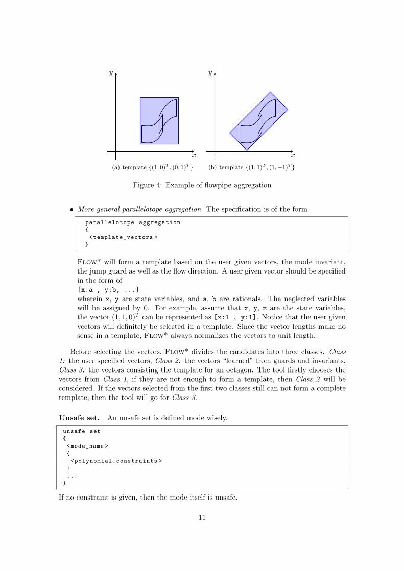
Aggregation. It is often necessary to aggregate a set of TMs to relieve the computa-tional burden in a reachability analysis task. Flow* computes a TM over-approximationfor the intersection of a set of TM flowpipes with a jump guard. Such an intersection isrepresented by a set of contracted TMs, to treat each of them individually however maylead to a very high computational cost. The main idea in Flow* is to first compute aparallelotope over-approximation based on a template which consists of a finite numberof vectors, and then translate it to an order 1 TM.
The orientation of a d-dimensional parallelotope can be determined by d linearly in-dependent vectors which are also the facet normals. To over-approximate a set by aparallelotope based on a given template, one may conservatively solve the optimizationproblems according to the template vectors on the set, and then compute a set of halfs-paces (represented by linear inequalities) whose intersection defines the parallelotope. Wegive an example in Figure 4. The two flowpipes can be over-approximated by a parallelo-tope according to the template {(1, 0)T , (0, 1)T }, or the template {(1, 1)T , (1,−1)T }. It isobvious that the template plays an important role in aggregation quality.
Flow* provides the following strategies to determine a template.
• Interval aggregation. One may simply useinterval aggregation
to tell Flow* to generate an interval or box aggregation.
10
x
y
(a) template {(1, 0)T , (0, 1)T }
x
y
(b) template {(1, 1)T , (1,−1)T }
Figure 4: Example of flowpipe aggregation
• More general parallelotope aggregation. The specification is of the form
parallelotope aggregation
{
<template_vectors >
}
Flow* will form a template based on the user given vectors, the mode invariant,the jump guard as well as the flow direction. A user given vector should be specifiedin the form of[x:a , y:b, ...]
wherein x, y are state variables, and a, b are rationals. The neglected variableswill be assigned by 0. For example, assume that x, y, z are the state variables,the vector (1, 1, 0)T can be represented as [x:1 , y:1]. Notice that the user givenvectors will definitely be selected in a template. Since the vector lengths make nosense in a template, Flow* always normalizes the vectors to unit length.
Before selecting the vectors, Flow* divides the candidates into three classes. Class1: the user specified vectors, Class 2: the vectors “learned” from guards and invariants,Class 3: the vectors consisting the template for an octagon. The tool firstly chooses thevectors from Class 1, if they are not enough to form a template, then Class 2 will beconsidered. If the vectors selected from the first two classes still can not form a completetemplate, then the tool will go for Class 3.
Unsafe set. An unsafe set is defined mode wisely.
unsafe set
{
<mode_name >
{
<polynomial_constraints >
}
...
}
If no constraint is given, then the mode itself is unsafe.
11

5 Output file
After completing a reachability computation task, Flow* stores all TM flowpipesalong with the state space definition and the computation tree in a flowpipe file. If thegiven safety property is not proved, the tool also dumps all (conservatively) detectedunsafe executions.
A flowpipe file of a continuous reachability problem is of the following form.
state var x, y, ... # state variable declaration
gnuplot octagon x , y # plot setting
cutoff 1e-15 # cutoff threshold
unsafe set # optional
{
<polynomial_constraints >
}
output name
continuous flowpipes
{
<Taylor_model_flowpipes >
}
A TM flowpipe is represented as
{
x = p + [a,b] # all components
...
local_t in [0,r] # domain of the TM
local_var_1 in [c,d]
...
}
wherein local t is the local time variable of the TM. It ranges in a time step interval.The TM variables are automatically named by the tool.
For hybrid reachability problems, the flowpipe files are of the form below.
state var x, y, ... # state variable declaration
<hybrid_state_space >
computation paths # sequences of modes
{
<paths >
}
gnuplot octagon x , y # plot setting
unsafe set # optional
{
<polynomial_constraints >
}
output name
12

hybrid flowpipes
{
<mode_name >
{
<Taylor_model_flowpipes >
}
...
}
The modes are organized by their visiting order in the reachability computation. Acomputation path is given by the form
m1 (n1 , [a1,b1]) -> m2 (n2 , [a2,b2]) -> ... -> mk;
which denotes a mode sequence from m1 to mk, such that the pair (ni , [ai, bi]) meansthat the jump is of the number ni and is executed at a time in [ai , bi].
Counterexample file. When Flow* fails to prove a safety property, it dumps allpossible unsafe executions as well as flowpipes to a counterexample file. If the reachabilityproblem is continuous, the unsafe TM flowpipes are kept in the following form.
{
starting time t # starting time of the flowpipe
{
... # TM flowpipe
}
...
}
For hybrid reachability problems, the counterexample file is of the following form.
<mode_name > # mode name
{
starting time t # local starting time of the flowpipe
{
... # TM flowpipe
}
...
computation path: # path leading to the unsafe flowpipes
m1 (n1 , [a1,b1]) -> m2 (n2 , [a2,b2]) -> ... -> mk;
}
...
References
[1] R. Alur, C. Courcoubetis, N. Halbwachs, T. A. Henzinger, P.-H. Ho, X. Nicollin,A. Olivero, J. Sifakis, and S. Yovine. The algorithmic analysis of hybrid systems.Theor. Comput. Sci., 138(1):3–34, 1995.
[2] X. Chen. Reachability Analysis of Non-Linear Hybrid Systems Using Taylor Models.PhD thesis, RWTH Aachen University, 2015.
13

[3] X. Chen, E. Abraham, and S. Sankaranarayanan. Taylor model flowpipe constructionfor non-linear hybrid systems. In Proceedings of the 33rd IEEE Real-Time SystemsSymposium (RTSS’12), pages 183–192. IEEE Computer Society, 2012.
[4] X. Chen, E. Abraham, and S. Sankaranarayanan. Flow*: An analyzer for non-linearhybrid systems. In Proceedings of the 25th International Conference on ComputerAided Verification (CAV’13), volume 8044 of Lecture Notes in Computer Science,pages 258–263. Springer, 2013.
[5] X. Chen, S. Schupp, I. Ben Makhlouf, E. Abraham, G. Frehse, and S. Kowalewski.A benchmark suite for hybrid systems reachability analysis. In Proceedings of the7th NASA Formal Methods Symposium (NFM’15), volume 9058 of Lecture Notes inComputer Science, pages 408–414. Springer, 2015.
[6] E. M. Izhikevich. Simple model of spiking neurons. IEEE Transactions on NeuralNetworks, 14(6):1569–1572, 2003.
[7] E. Klipp, R. Herwig, A. Kowald, C. Wierling, and H. Lehrach. Systems Biology inPractice: Concepts, Implementation and Application. Wiley-Blackwell, 2005.
[8] K. Makino and M. Berz. Suppression of the wrapping effect by taylor model-basedverified integrators: Long-term stabilization by preconditioning. International Journalof Differential Equations and Applications, 10(4):353–384, 2005.
14