user's guide for life2's rainflow counting algorithm

SANDIA REPORT SAND90–2259 ● UC–261

Unlimited Release

Printed January 1991

User’s Guide for LIFE2’s Rainflow Counting Algorithm

L. L. Schluter, H. J. Sutherland

Prepared by

Sandia National Laboratories Albuquerque, New Mexico 87185 and Livermore, California 94550 for the United States Department of Energy under Contract DE-AC04-76DPO0789

SFYCOCI(S-81 )

Issued by Sandia National Laboratories, operated for the United States Department of Energy by Sandia Corporation. NOTICE: This report was prepared as an account of work sponsored by an agency of the United States Government. Neither the United States Govern- ment nor any agency thereof, nor any of their employees, nor any of their contractors, subcontractors, or their employees, makes any warranty, express or implied, or assumes any legal liability or responsibility for the accuracy, completeness, or usefulness of any information, apparatus, product, or process disclosed, or represents that its use would not infringe privately owned rights. Reference herein to any specific commercial product, process, or service by trade name, trademark, manufacturer, or otherwise, does not necessarily constitute or imply its endorsement, recommendation, or favoring by the United States Government, any agency thereof or any of their contractors or subcontractors. The views and opinions expressed herein do not necessarily state or reflect those of the United States Government, any agency thereof or any of their contractors.

Printed in the United States of America. This report has been reproduced directly from the best available copy.

Available to DOE and DOE contractors from Office of Sclentlflc and Technical Information PO BOX 62 Oak Ridge, TN 37831

Prices available from (615) 576-8401, FTS 626-8401

Available to the public from National Technical Information Service US Department of Commerce 5285 Port Royal Rd Springfield, VA 22161

NTIS price codes Printed copy: A03 Microfiche copy: AO1

USER’S GUIDE FOR LIFE2’S

RAINFLOW COUNTING ALGORITHM*

by

L. L. Schluter

and

H. J. Sutherland

Wind Energy Research Division Sandia National Laboratories

Albuquerque, NM 87185

ABSTRACT

The LIFE2 computer code is a fatigue/fracture code for the analysis of wind turbine components. The numerical formulation of the code uses a series of cycle count matrices to describe the cyclic stress states imposed upon the component. In this formulation, each stress cycle is counted, or “binsed,’’according to the magnitude of its mean stress and cyclic stress components and by the operating condition of the turbine. This paper describes a set of numerical algorithms that have been incorporated into the LIFE2 code. These algorithms determine the cycle count matrices for a turbine component using stress-time histories of the imposed stress states. A user’s manual is included that explains the operation of these algorithms. An example session illustrates the use of these algorithms.

*This work is supported by the U.S. Department of Energy at Sandia National Laboratories under contract DE-AC04-76DPO0789.

The authors wish to thank P. S. Veers and D. P. Burwinkle for their help in implementing and checking these algorithms.

-4-

TABLE OF CONTENTS

ACKNOWLEDGMENTS . . . . . . . . . . . . . . . . . . . . . . . . . . . . . . . . . . . . . . . . . . . . . . . . . . . . . . . . . . . . . . . . . . . . . . . . . . . . . . . .

INTRODUCTION . . . . . . . . . . . . . . . . . . . . . . . . . . . . . . . . . . . . . . . . . . . . . . . . . . . . . . . . . . . . . . . . . . . . . . . . . . . . . . . . . . . . . . . . . . .

BACKGROUND INFORMATION . . . . . . . . . . . . . . . . . . . . . . . . . . . . . . . . . . . . . . . . . . . . . . . . . . . . . . . . . . . . . Pre-Count Algorithms . . . . . . . . . . . . . . . . . . . . . . . . . . . . . . . . . . . . . . . . . . . . . . . . . . . . . . . . . . . . . . . . . . . . . . . . . . . . . .

Peak-Valley Selection . . . . . . . . . . . . . . . . . . . . . . . . . . . . . . . . . . . . . . . . . . . . . . . . . . . . . . . . . . . . . . . . . . . . Filter . . . . . . . . . . . . . . . . . . . . . . . . . . . . . . . . . . . . . . . . . . . . . . . . . . . . . . . . . . . . . . . . . . . . . . . . . . . . . . . . . . . . . . . . . . . . . . . . .

Rainflow Counting Algorithm . . . . . . . . . . . . . . . . . . . . . . . . . . . . . . . . . . . . . . . . . . . . . . . . . . . . . . . . . . . . . . . . Post-Count Algorlthm . . . . . . . . . . . . . . . . . . . . . . . . . . . . . . . . . . . . . . . . . . . . . . . . . . . . . . . . . . . . . . . . . . . . . . . . . . . . . .

REFERENCE WUAL . . . . . . . . . . . . . . . . . . . . . . . . . . . . . . . . . . . . . . . . . . . . . . . . . . . . . . . . . . . . . . . . . . . . . . . . . . . . . . . The Time Series Input Data File . . . . . . . . . . . . . . . . . . . . . . . . . . . . . . . . . . . . . . . . . . . . . . . . . . . . . . . . . . . Data Files for the Stress States Module . . . . . . . . . . . . . . . . . . . . . . . . . . . . . . . . . . . . . . . . . . . . . . . Finding the Peaks and Valleys in the Time Series . . . . . . . . . . . . . . . . . . . . . . . . . . . . . . Usin the Race Track Filter

f . . . . . . . . . . . . . . . . . . . . . . . . . . . . . . . . . . . . . . . . . . . . . . . . . . . . . . . . . . . . . . . . . . .

Disp aying Matrix Information . . . . . . . . . . . . . . . . . . . . . . . . . . . . . . . . . . . . . . . . . . . . . . . . . . . . . . . . . . . . . . . Documenting Units . . . . . . . . . . . . . . . . . . . . . . . . . . . . . . . . . . . . . . . . . . . . . . . . . . . . . . . . . . . . . . . . . . . . . . . . . . . . . . . . . . .

EXAMPLE SESSION . . . . . . . . . . . . . . . . . . . . . . . . . . . . . . . . . . . . . . . . . . . . . . . . . . . . . . . . . . . . . . . . . . . . . . . . . . . . . . . . . . . . . . .

SUMMARY . . . . . . . . . . . . . . . . . . . . . . . . . . . . . . . . . . . . . . . . . . . . . . . . . . . . . . . . . . . . . . . . . . . . . . . . . . . . . . . . . . . . . . . . . . . . . . . . . . . . . . . .

REFERENCES . . . . . . . . . . . . . . . . . . . . . . . . . . . . . . . . . . . . . . . . . . . . . . . . . . . . . . . . . . . . . . . . . . . . . . . . . . . . . . . . . . . . . . . . . . . . . . . . . .

APPENDIX . . . . . . . . . . . . . . . . . . . . . . . . . . . . . . . . . . . . . . . . . . . . . . . . . . . . . . . . . . . . . . . . . . . . . . . . . . . . . . . . . . . . . . . . . . . . . . . . . . . . . . . .

page

4

6

7 7 7 9

1;

11 11 12 16 16 17 18

19

25

26

27

-5-

INTRODUCTION

The LIFE2 computer code is a fatigue/fracture analysis code specifically 2 designed fortheanalysis ofwind turbine components (1,2). It isa P -

compatible Fortran code that is written in a top-down modular format with a “user friendl “ interactive interface. In this numerical formulation, an “S-

{ n“ fatigue ana ysis is used to describe the initiation, growth and coalescence of micro-cracks into macro-cracks. A linear, “da/dn” fracture analysis is used to describe the growth of a macro-crack.

In the LIFE2 formulation, each stress cycle imposed on the turbine component is characterized by the magnitude of its mean stress and cyclic (range or alternating) stress components and by the operating condition of the turbine. This paper describes a set of numerical algorithms that permits the code to analyze stress-time histories of component stress states. The main algorithm is a rainflow counting algorithm. It defines a stress cycle to be a closed stress/strain hysteresis loop. It determines the mean stress level and the range for each stress cycle in a given stress-time history.

These algorithms have been incorporated into the LIFE2 code. A user’s manual is included in this paper to illustrate their operation. An example session is included for reference. A detailed description of how the algorithms have been implemented with Fortran 77 is in Schluter (3).

-6-

BACKGROUND INFORMATION

The prime algorithm used here is a rainflow counting algorithm (4). It defines a stress cycle to be a closed stress/ strain hysteresis loop. It determines the mean stress level and the range for each stress cycle m the histogram. To illustrate the use of this al orithm, consider the typical

E stress-time history for a turbine components own in Fig. 1. As this history is being used for illustrative purposes only, the stresses have been normalized.

3

2

1

0

-1

-2

-3

0 100 200

Time, sec

Figure 1 Typical stress-time history data

Pre-Count Al~orithms

Several auxiliary al~orithms are used to support the rain-flow counting. The initial set of algorithms prepares the full time series data for counting by selecting peaks and valleys and discarding ‘Small” stress cycles. After counting, other algorithms record and store the cycle count data in an appropriate format for the LIFE2 analysis.

Peak-Valley Selection. The first algorithm identifies peaks and valleys in the data record by scanning for changes in the sign of the slope.

-7-

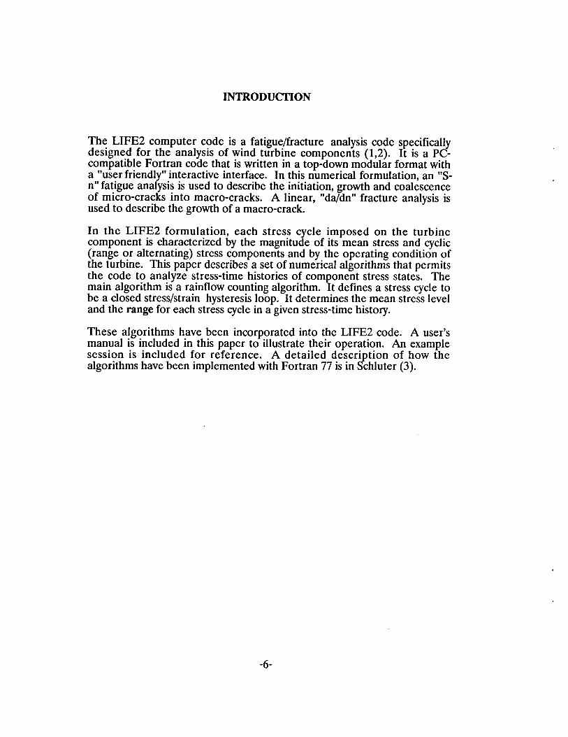
Typically, the data contained in this class of stress records are taken at umform time intervals. This constant-time-interval sampling technique may or may not record actual extrema in the data, because the extrema may be ‘kquared off”; e. .,

f the peak at a~proximately 185 seconds in Fig. 2 (an

expanded view o the data shown m Fig. 1). To obtain a better estimate of the actual extrema at a change in the slope, a parabola is fit to the three data points nearest that change. The extrema determined using this curve- fitting technique are shown as squares in Fig. 2.

As shown in Fig. 2, this technique for choosing the extrema mayor may not significantly change the maxima recorded in the data. In particular, the extrema recorded in the data record at approximately 140, 150, 165 and 180 seconds in Fig. 2 are very close to the true eaks, because the sampling technique has not squared off their peaks. L owever, when the extrema have been squared off, as with the peak at approximately 185 seconds, the extrema are significantly increased by this curve fitting technique producing a peak much closer to the true value.

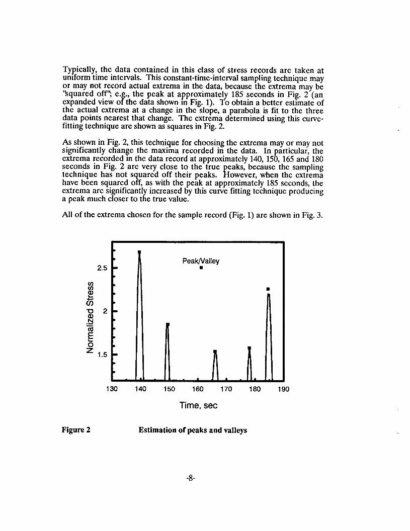
All of the extrema chosen for the sample record (Fig. 1) are shown in Fig. 3.

Figure 2

2.5

2

1.5

●

●

m

●

●

w

●

m

●

●

●

●

m

●

●

Peak/Valley 9

130 140 150

Estimation

160 170 180 190

Time, sec

of peaks and valleys

-8-

o 100 200

Time, see

Figure 3 Selected peaks and valleys (no filter)

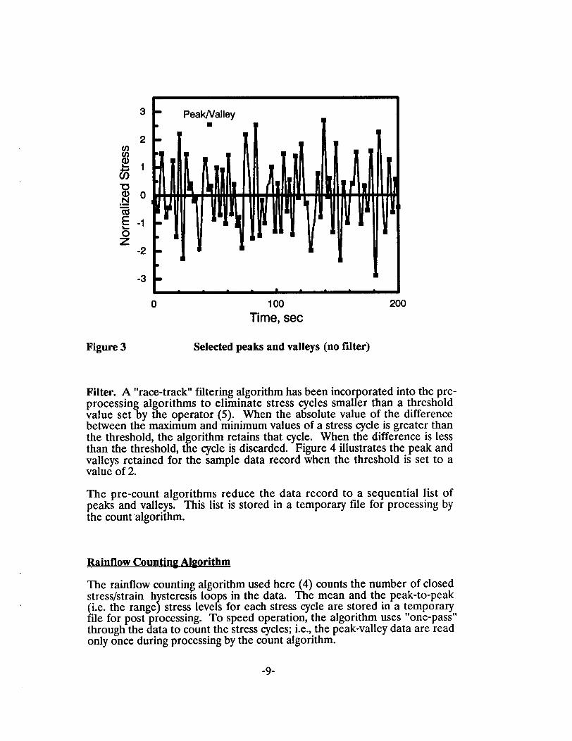
Filter. A “race-track” filtering algorithm has been incorporated into the pre- processing algorithms to eliminate stress cycles smaller than a threshold value set by the operator (5). When the absolute value of the difference between the maximum and minimum values of a stress cycle is greater than the threshold, the al orithm retains that cycle. When the difference is less

i than the threshold, t e cycle is discarded. Figure 4 illustrates the peak and valleys retained for the sample data record when the threshold is set to a value of 2.

The pre-count algorithms reduce the data record to a sequential list of peaks and valleys. This list is stored in a temporary file for processing by the count ‘algorithm.

Rainflow Countirw Ahzorithm

The rainflow counting algorithm used here (4) counts the number of closed stress/strain h steresls loops in the data. The mean and the peak-to-peak

T (i.e. the range stress levels for each stress cycle are stored in a temporary file for post processing. To speed operation, the algorithm uses “one-pass” through the data to count the stress cycles; i.e., the peak-valley data are read only once during processing by the count algorithm.

-9-

3F Peak/Vallev

u a N .- 73 E 5 z

2

1

0

-1

-2

-3

m

●

m

●

m

J

w m

Threshold Set Equal to 2

Ill 0 100 200

Time, sec

Figure 4 Selected peaks and valleys with a threshold of 2

Post-Count Ahzorithm

The final algorith maps each stress cycle into a cycle count matrix that can 1? be processed by he LIFE2 code. The algorithm sorts the stress cycle data

into bins that are functions of mean stress level and the range.

The cycle counts from a data record may be used to create a new cycle count matrix, or they may be added to an existing cycle count matrix, at the discretion of the operator.

-1o-

This section describes the format of the time series data file and how the code creates and maintains the data files containing the counted cycles. Also discussed are the pre-count algorithms for finding the peaks and valleys in the time series data file and for filtering out small stress cycles (the race-track filter algorithm).

The pre-count, rainflow counting, and post-count algorithms have been incorporated into the LIFE2 code in the stress states module. The operator may input operational stresses, buffeting stresses, or start/ stop stresses. The algorithms have been added as Option 4 under these respective menus (see Schluter and Sutherland (1) for a comrJete description of the menuirw ~ystem used by the LIFE2 code):

. .

This section discusses states data files, the information contained

The Time Series Immt

the time series file, the basic structure of the stress manipulation of the data files, and the display of in the data files.

Data File

The file that contains the stress data to be rainflow counted is referred to as the time series data file or simply time series. LIFE2 will prompt the operator for the name of the time series file and the length of the time series in seconds.

The time series data file needs to be created as a sequential file that has one stress ent~ per line. The stress entry may be any desired format (e.g., real, exponential, etc.). The following is an example of a time series data file with nine entries:

-5.2 4.12 1.34 3.02 2.8 0.55 -1.03 -1.75 -0.65

The length of the data file is limited only by the amount of free storage space on the computer’s hard disc.

-11-

LIFE2 creates and use sdata files to transfer data between computational modules and to archive data. Their operation is transparent to the operator. However, it is necessary to understand the basic structure of the stress states data files in order to understand how the LIFE2 code manipulates them.

The data files for the stress states module consist of a series of two- dimensional cycle count matrices (mean vs. cyclic stress where the clic

7 stress may either be the alternating stress value or the range stress va ue). When working with operational or buffeting stresses each matrix corresponds to a particular wind speed interval (i.e., 5 to 10 mph). When working with start/ stop stresses, each matrix corresponds to a particular start or stop condition. An example cycle count matrix is shown in Fig. 5. When adding data to an existing data file, the matrices that currently exist are listed. The o erator may add the data to an existing matrix or specify

E that a new matrix e created.

Mean Stress Array

3 6 9 12 18 21 24 27 30 33

5

10

15

20

25

30

35

40

Figure 5

10 40 66 138 150 198 84 28 10 2

4 2 16 28 46 38 16 2

6 16 40 22 8

36 32 26 2

2 14 20 10 2

2 4 2

2 2 2

2

Example matrix

-12-

Each time series that is inserted into a data file isconsidered to be one record. The number of records contained in a matrix is incremented by one for each time series added. Each matrix may have up to 50 stress intervals for both the mean and the cyclic stresses.

When creating a new matrix, the program will ask the operator for the desired resolutions of the stress intervals in the stress arrays. The arrays are calculated so that the maximum value found in the time series data will always be included within the matrix. Intervals are added to the stress arrays until the maximum is included or the number of intervals is 50. The first stress interval will contain all values less than a specific stress level. All other intervals have lower and upper bounds. For example, in Fig. 5 the mean stress array has 10 intervals with a resolution of 3. The cychc stress array has 8 intervals with a resolution of 5. For the mean stress array the first interval is associated with all values less than or equal to 3. The second interval is associated with the range of values greater than 3 and less than or equal to 6.

It should be noted that the smaller the resolution the smaller the range of values that can be covered by the matrix. For example, with a 1 MPa resolution the matrix will cover a total of 50 MPa. With a.5 MPa resolution the matrix will cover a total of 25 MPa.

The rainflow counting algorithms will record the mean stress value and the range for each

? cle. The program will then insert this information into the

matrix. In Fig. there are 10 cycles with a mean value less than or equal to 3 and a range value less than or equal to 5; there are 40 cycles with a mean value greater than 3 but less than or equal to 6 and a range value less than 5, etc.

Once a matrix has been set up, time series data may be added to it whenever desired. However, the resolution cannot be changed. Since large stress values cause significantly more damage than small stress values, it is important that the matrix always contain the maximum values for both the mean and cyclic stresses. If the current maximum for one of the stress arrays is less than the maximum value found in a time series, the matrix will be added to or shifted so that the new maximum is included. If the stress array does not have 50 intervals, then intervals will be added until the maximum is contained in the matrix. An example of adding a

7 clic stress

interval to the matrix in Fig. 5 is shown in Fig. 6. If a new cyc e is found with a mean stress of 11.5 and cyclic stress of 41.8 then the matrix must be expanded. In this case a new cyclic interval is added as shown in Fig. 6.

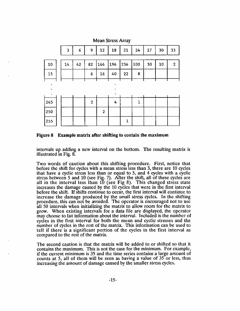
If the stress array already contains 50 intervals, then the matrix is shifted. An example of this is shown in Fig. 7. The matrix in Fig. 7 has a cyclic stress array that contains 50 intervals. If a cycle is found that has a mean value of 19.25 and cyclic value of 252.1, then the matrix must be shifted. This is done by summing the first two rows and then shifting the

-13-

Mean Stress Array

5

10

15

20

25

30

35

40

45

3 6 9 12 18 21 24

*

10 40 66 138

4 2 16 28

6 16

36

2 14

2

2

1

:

150 198

46 38

40 22

32 26

20 10

42

-1-J 2 I

m 84 28 10 2

16 2

8

2

2

2

Figure 6 Adding a mean stress interval

Mean Stress Array

3 6 9 12 18 21 24 27 30 33

E 5

10

E 245

250

BE 10 40 66

4 2 16

138

28 +

150 198

46 38 E 84 28

16 2

10 3 2

I

2 4 1

2

Figure 7 Example matrix before shifting to contain the maximum

Mean Stress Array

3 6 9 12 18 21 24 27 30 33

BYE E=EEEEE .

.

H 245 2 4 1

250 2

255 1

Figure 8 Example matrix atler shifting to contain the maximum

intervals up adding a new interval on the bottom. The illustrated m Fig. 8.

Two words of caution about this shifting procedure.

resulting matrix is

First, notice that before the shift for cycles with a mean stre;s iess than 3, there are 10 cycles that have a cyclic stress less than or equal to 5, and 4 cycles with a cyclic stress between 5 and 10 (see Fig. 7). After the shift, all of these cycles are all in the interval less than 10 (see Fig 8). This changed stress state increases the damage caused by the 10 cycles that were in the first interval before the shift. If shifts continue to occur, the first interval will continue to increase the damage produced by the small stress cycles. In the shifting procedure, this can not be avoided. The operator is encouraged not to use all 50 intervals when initializing the matrix to allow room for the matrix to grow. When existing intervals for a data file are displayed, the operator may choose to list information about the interval. Included is the number of cycles in the first interval for both the mean and cyclic stresses and the number of cycles in the rest of the matrix. This information can be used to tell if there is a significant portion of the cycles in the first interval as compared to the rest of the matrix.

The second caution is that the matrix will be added to or shifted so that it contains the maximum. This is not the case for the minimum. For example, if the current minimum is 35 and the time series contains a large amount of counts at 5, all of them will be seen as having a value of 35 or less, thus increasing the amount of damage caused by the smaller stress cycles.

-15-

In both of the above cases it should be noted that small stress cycles will probably not affect the lifetime calculation since they cause much less damage than large stress cycles. If an effect is seen, it will be that the lifetime calculation will always be a conservative estimate.

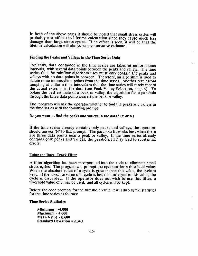
Findin~ the Peaks and Vallevs in the Time Series Data

Typically, data contained in the time series are taken at uniform time intervals, with several data points between the peaks and valleys. The time series that the rainflow algorithm uses must only contain the peaks and valleys with no data points in between. Therefore, an algorithm is used to delete these intermediate points from the time series. Another result from sampling at uniform time intervals is that the time series will rarely record the actual extrema in the data (see Peak-Valley Selection, page 4). To obtain the best estimate of a peak or valley, the algorithm fits a parabola through the three data points nearest the peak or valley.

The program will ask the operator whether to find the peaks and valleys in the time series with the following prompt:

Do you want to find the peaks and valleys in the data? (Y or N)

If the time series already contains only peaks and valleys, the operator should answer ‘N’ to this prompt. The parabola fit works best when there are three data points near a peak or valley. If the time series already contains only peaks and valleys, the parabola fit. may lead to substantial errors.

Usirw the Race- Track Filter

A filter algorithm has been incorporated into the code to eliminate small stress cycles. The program will prompt the operator for a threshold value. When the absolute value of a cycle is greater than this value, the cycle is kept. If the absolute value of a cycle is less than or equal to this value, the cycle is discarded. If the operator does not wish to use this filter, a threshold value of O may be used, and all cycles will be kept.

Before the code prompts for the threshold value, it will display the statistics for the time series as follows:

Time Series Statistics

Minimum = -4.000 Maximum = 4.000 Mean Value = 0.6S0 Standard Deviation = 2.340

-16-

One recommendation for a threshold value is the standard deviation of the time series. This value will filter out much of the noise while keeping the

‘1 cles that do most of the damage. For a complete discussion of why this is

t e case please see Veers (6).

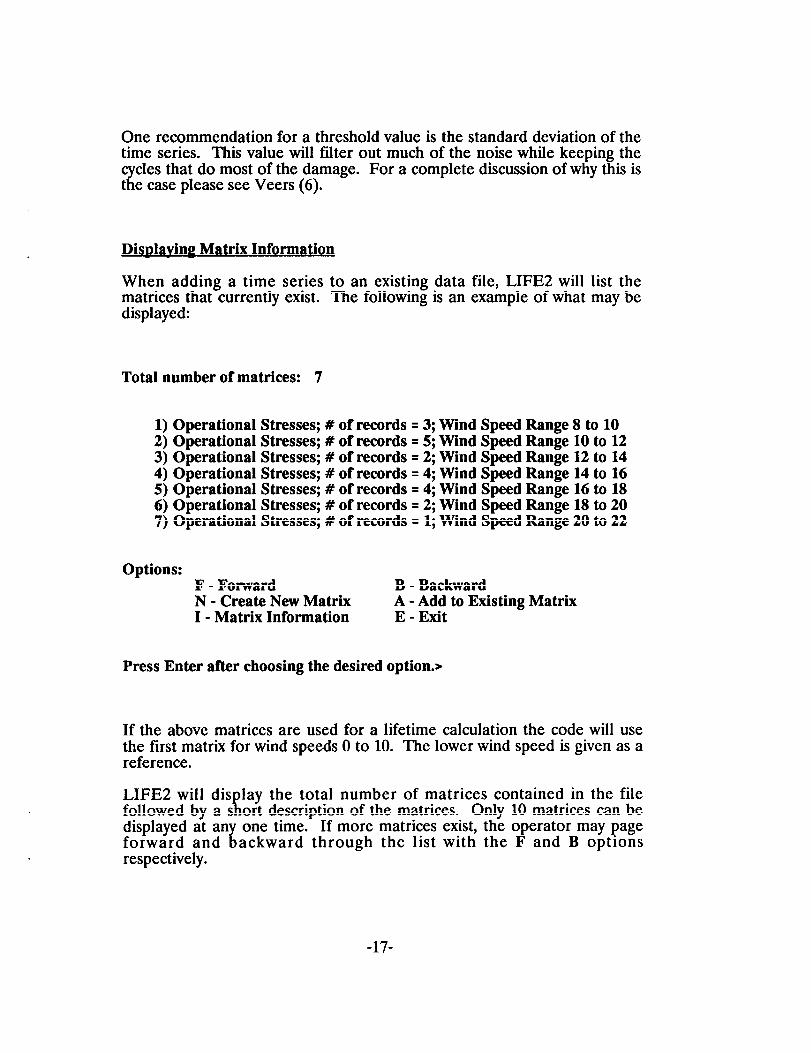
Dis~lavin~ Matrix Information

When adding a time series to an existing data file, LIFE2 will list the matrices that currently exist. The following is an example of what may be displayed:

Total number of matrices: 7

1) Operational 2) Operational 3) Operational 4) Operational 5) Operational 6) Operational 7) Operational

Stresses; #of records =3; Wind Speed Range 8 to 10 Stresses; #of records =5; Wind Speed Range 10 to 12 Stresses; #of records =2; Wind Speed Range 12 to 14 Stresses; #of records =4; Wind Speed Range 14 to 16 Stresses; #of records =4; Wind Speed Range 16 to 18 Stresses; #of records =2; Wind Speed Range 18 to 20 Stresses; #of records = 1; Wind Speed Range 20 to 22

Options: F - Forward B - Backward N - Create New Matrix A - Add to Existing Matrix I - Matrix Information E - Exit

Press Enter after choosing the desired option.>

If the above matrices are used for a lifetime calculation the code will use the first matrix for wind speeds O to 10. The lower wind speed is given as a reference.

LIFE2 will dis lay the total number of matrices contained in the file [ followed by a s ort description of the matrices. Only 10 matrices can be

displayed at any one time. If more matrices exist, the operator may page forward and backward through the list with the F and B options respectively.

-17-

If a time series is to be inserted into a matrix that exists, then the A option is chosen. The code will prompt for the number corresponding to the desired matrix.

If a new matrix must be created for the time series data, then o tion N is f chosen. The code will then prom t for the wind range correspon ing to the

J matrix and a new matrix is create .

The operator may choose to display more information on a particular matrix. To do this option I is chosen. LIFE2 will then display a screen similar to the following:

Number of Records: 5

Units of Wind Speed are mph Lower Wind Speed = 10.00 Upper Wind Speed = 12.00

Units of Stress are KPa

Number of Mean Stress Intervals= 10 Minimum Mean Stress = 0.0 Maximum Mean Stress = 50.00

Number of Cyclic Stress Intervals= 20 Minimum Cyclic Stress = 10.0 Maximum Cyclic Stress = 110.00

Number of Counts in the first mean interval = O Number of Counts in the first cyclic interval = O Number of Counts in rest of matrix= 103

Press ENTER to continue

When LIFE2 continues, it will redisplay the matrices that currently exist.

Documenting Unit$

The LIFE2 code is unit insensitive. The user must assure that compatible units are used throughout the calculation. The code will ask for the units being used in the calculation so that they may be documented in the data files.

-18-

EXAMPLE SESSION

The followin$ illustrates an example session using the rainflow counting algorithms with operational stress data. In the session, a new data file is created and time series data are rainflow counted and placed into a matrix. Next another time series data set that corresponds to a different wind speed is counted and placed in a different matrix. Then time series data are added to the first matrix. Finally the data file is saved in the operational stresses library. Sessions for entering start/ stop stresses and buffeting stresses are similar.

In the example, LIFE2 code prompts are written in bold letters. The operator’s responses to the prompts are written in italics.

The time series files used in this example are shown in the appendix. These are very simple files and are meant for illustrative pu~oses. Also shown in the appendix is the data file that is created after each time series is inserted.

After choosing the rainflow counting option from the operational stresses menu, the following prompts appear:

>>> Rainflow Counting <<<

This menu allows the operator to use the rainflow counting algorithms on a time series data file.

Your options at this level are

1) Create a New Data File 2) Add Data to an Existing Data File

9) Return to the Operational Stresses Menu

Enter the number of the desired option.>1

Enter the title of the data tile no longer than 72 characters 13ample Data File for the Rainflow Manual

Enter the units of stress.>MPa

-19-

Enter the units of wind speed.wn/s

Enter the lower range of wind speed for this data set.> 1(1

Enter the upper range of wind speed for this data set.>12

Enter the name of the time series data file. xawnpleldat

Enter the length of the time series in seconds.>30

Do you wish to find the peaks and valleys in the time series?(Y or N)>Y

. . . ..Calculating Statistics for the time series


Minimum = -4.000 Maximum = 4.000 Mean Value = 0.6S0 Standard Deviation ❑ 2.340

Input the Racetrack Filter threshold value.(0 for no tilter)>O

The extreme values for the mean stress are

Minimum = 0.000

Maximum = 3.000

Enter the resolution for the mean stress intervals.>.5

-20-

The extreme values for the cyclic stress are

Minimum = 1.000

Maximum = 8.000

Enter the resolution for the cyclic stress intervals.>1

Do you wish to add another time series to this data tile. (1’ or N)>Y


1) Operational Stresses; # Records ❑ 1; Wind Speed Range 10 to 12

Options: F - Page Forward B - Page Backward N - Create New Matrix A - Add to Existing Matrix I - Matrix Information E - Exit

Enter the desired option.>n

Input the lower range of wind speed for this data set.>12

Input the upper range of wind speed for this data set.>14

Enter the name of the time series data file.>[email protected]




-21-


Minimum = -5.000 Maximum = 5.000 Mean Value = 0.500 Standard Deviation = 2.690

Input the Racetrack Filter threshold value.(0 for no filter)>fl

The extreme values for the mean stress are

Minimum = -1.49082600

Maximum = 2.85526500

Enter the resolution for the mean stress intervals.>. 75

The extreme values for the cyclic stress are

Minimum = 1.03276900

Maximum = 10.07811000

Enter the resolution for the cyclic stress intervals.>2

Do you wish to add another time series to this data file.(Y or N)>Y


1) Operational Stresses; # of records = 1; Wind Speed Range 10 to 12 2) Operational Stresses; #of records = 1; Wind Speed Range 12 to 14

Options: F - Page Forward B - Page Backward N - Create New Matrix A - Add to Existing Matrix I - Matrix Information E - Exit

Enter the desired option.>a

-22-

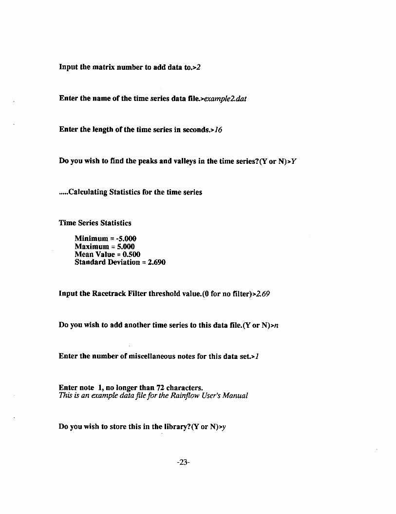
Input the matrix number to add data to.>2

Enter the name of the time series data [email protected]





Minimum = -5.000 Maximum = 5.000 Mean Value = 0.500 Standard Deviation = 2.690

Input the Racetrack Filter threshold value.(0 for no tllter)>2.69

Do you wish to add another time series to this data file.(Y or N)wz

Enter the number of miscellaneous notes for this data se~>l

Enter note 1, no longer than 72 characters. This is an example data file for the Rainjlow Userh Manual

Do you wish to store this in the library?(Y or N)>y

-23-

The following is a list of data files currently available in the library:

1) 17M45R 2) 17M36R 3) 34M28R 4) 34M36R

Enter a 1-6 character name under which to store the tile just created, revised, or added.wnanual

-24-

A set of algorithms that rainflow count time-series stress data has been incorporated into the LIFE2 fatigue/ fracture analysis code. Sup ort

b algorithms that structure the data in a format compatible with the LI E2 code have also been implemented. This report describes the rainflow counting algorithms and the support algorithms.

A user’s manual is included that describes the format of the time series files and how the code manipulates the data files, and shows an example session with the code. For anyone interested in how the al orithms have been

! implemented usin Fortran 77, a programmer’s uide 3) is available. The programmer’s f f gui e describes the major design ecisions that were made in Implementing the algorithms and details of the subroutines used to implement the algorithms.

-25-

REFERENCES

1. Schluter, L. L. and Sutherland, H. J., Reference Manual for the LIFE2 co DUt ode , SAND89-1396, Sandia National Laboratories, Albuquerqfle, N; September 1989.

2. Sutherland, H. J., Analytical Framework for the LIFE2 Comtmter Code, SAND89-1397, Sandia National Laboratories, Albuquerque, NM, September 1989.

3. Schluter, L. L., Pr r mm r’ i op a e s Gu de for the LIFE2 Rainflow Countin~ Alwmithm$, SAN90-2260, Sandia National Laboratories, Albuquerque, ~ M, August 1990.

4. Downing, S. D., and Socie, D. F., ‘Simple Rainflow Counting Algorithms,” IntemationalJoumal of Fatigue, Vol. 4, N. 1, 1982, pp. 31-40.

5. Veers, P. S., Winterstein, S. R., Nelson, D. V. and Cornell, C. A., “Variable Amplitude Load Models for Fati ue Damage and Crack Growth,”

!3 Development of Fatigue Loading Spectra, A TM STP 1006, J. M. Potter and R. T. Watanabe, eds., 1989, pp. 172-197.

6. Veers, P. S., Fati~ue Crack Growth Due to Random Loading, SAND87-2039, Sandia National Laboratories, Albuquerque, NM, November 1987.

-26-

Appendix

Example Session Files

The following appendix shows the time series data files used for the example session and the stress state data file that results.

-27-

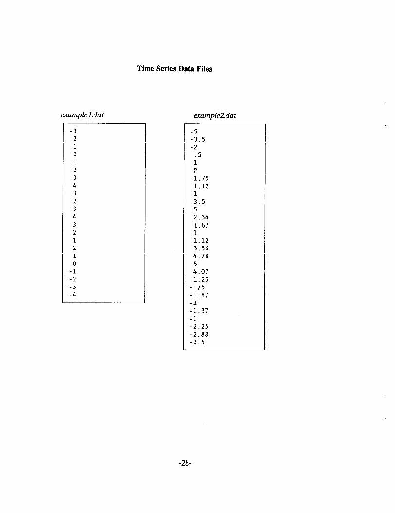
txamplel.dat

Time Series Data Files

-3 -2 -1 0 1 2 3 4 3 2 3 4 3 2 1 2 1 0 -1 -2 -3 -4

twample2.dat

-5 -3.5 -2 .5 1 2 1.75 1.12 1 3.5 5 2.34 1.67 1 1.12 3.56 4.28 5 4.07 1.25 -.75 -1.87 -2 -1.37 -1 -2.25 -2.88 -3.5

-28-

Format of Stress States Data File

The title of the file Stress Units Time Units Wind Speed Units Data Characterized by one Mean Stress - ‘y’ or ‘n’ Number of Wind Speed Matrices - N Title of Matrix #1 Upper bound of wind speed for data set #1 Time Matrix for series #1 of cvcle counts (WC) Number of Mean Stress Entri& -1 Number of Cyclic Stress Entries - J Mean Stress #l Mean Stress #2

Mean S~ress #I Qclic Stress #1 Cyclic Stress #2

.

. Cyclic Stress #J Cycles to failure(l,l) Cycle Count(l,2)

Cycle Count (lJ)

Cycle C&nt (1,1) Cycle Count(I,2)

.

Cycle Count (IJ) Title of Data Set #2*

Title of Data Set #N*

Numbe; of Miscellaneous Notes - x Note #1

Mean Stress #3 Mean Stress #4

Cyclic Stress #3 Cyclic Stress #4

Cycles to failure(l,3) Cycle Count (1,4)

Cycle Count (1,3) Cycle Count (1,4)

Note #x

-29-

The following is the Stress States Data File after the first insertion.

Example Data File for the Rainflow Manual MPa seconds nds n

~perational Stresses # Records = 1; Wind Speed Range 10 to 12 .12000000E+02 .30000000E+02 7 8 .OOOOOOOOE+OO .50000000E+O0 .1OOOOOOOE+O1 .15000000E+01 .20000000E+01 .25000000E+01 .30000000E+01 .100000000+01 .20000000E+01 .30000000E+01 .40000000E+01 .50000000E+01 .60000000E+01 .70000000E+01 .80000000E+01 .000000000+00 .OOOOOOOOE+OO .OOOOOOOOE+OO .OOOOOOOOE+OO .OOOOOOOOE+OO .OOOOOOOOE+OO .OOOOOOOOE+OO .1OOOOOOOE+OO .000000000+00 .OOOOOOOOE+OO .OOOOOOOOE+OO .OOOOOOOOE+OO .OOOOOOOOE+OO .OOOOOOOOE+OO .OOOOOOOOE+OO .OOOOOOOOE+OO .000000000+00 .OOOOOOOOE+OO .OOOOOOOOE+OO .OOOOOOOOE+OO .OOOOOOOOE+OO .OOOOOOOOE+OO .OOOOOOOOE+OO .OOOOOOOOE+OO .100000000+01 .OOOOOOOOE+OO .OOOOOOOOE+OO .OOOOOOOOE+OO .OOOOOOOOE+OO .OOOOOOOOE+OO .OOOOOOOOE+OO .OOOOOOOOE+OO .000000000+00 .OOOOOOOOE+OO .OOOOOOOOE+OO .OOOOOOOOE+OO .OOOOOOOOE+OO .OOOOOOOOE+OO .OOOOOOOOE+OO .OOOOOOOOE+OO .000000000+00 .OOOOOOOOE+OO .OOOOOOOOE+OO .OOOOOOOOE+OO .OOOOOOOOE+OO .OOOOOOOOE+OO .OOOOOOOOE+OO .OOOOOOOOE+OO .000000000+00 .1OOOOOOOE+O1 .OOOOOOOOE+OO .OOOOOOOOE+OO .OOOOOOOOE+OO .OOOOOOOOE+OO .OOOOOOOOE+OO .OOOOOOOOE+OO

o

-30-

The following is the Stress States Data File after the second insertion.

Example Data File for the Raintlow Manual MFa seconds In/s n 2 Operational Stressev # Records = 1; Wind Speed Range 10 to 12

.12000000E+02

.30000000E+02 7 8 .OOOOOOOOE+OO .50000000E+O0 .1OOOOOOOE+O1 .15000000E+01 .20000000E+01 .25000000E+01 .30000000E+01 .MMOOOOO+OI .20000000E+OI .30000000E+OI .40000000E+OI .50000000E+01 .60000000E+01 .70000000E+01 .80000000E+01 .000000000+00 .OOOOOOOOE+OO .WOOOOOOE+OO .OOOOOOOOE+OO .OOOOOOOOE+OO .OOOOOOOOE+OO .OOOOOOOOE+OO .1OOOOOOOE+OO .OOOOOOOOO+OO .OOOOOOOOE+OO .0000OOWE+OO .OOOOOOOOE+OO .OOOOOOOOE+OO .OOOOOOOOE+OO .00W0OOOE+OO .OOOOOOOOE+OO .000000000+00 .0000OOOOE+OO .0000OOWE+OO .OOOOOOOOE+OO .OOOOOOOOE+OO .OOOOOOOOE+OO .OOOOOOOOE+OO .OOOOOOOOE+OO .100000000+01 .OOOOOOOOE+OO .OOOOOOOOE+OO .OOOOOOOOE+OO .OOOOOOOOE+OO .OOOOOOOOE+OO .OOOOOOOOE+OO .OOOOOOOOE+OO .000000000+00 .OOOOOOOOE+OO .OOOOOOOOE+OO .OOOOOOOOE+OO .OOOOOOOOE+OO .OOOOOOOOE+OO .OOOOOOOOE+OO .OOOOOOOOE+OO .000000000+00 .OOOOOOOOE+OO .OOOOOOOOE+OO .OOOOOOOOE+OO .OOOOOOOOE+OO .OOOOOOOOE+OO .OOOOOOOOE+OO .OOOOOOOOE+OO .OOOOOOOOO+OO .1 OOOOOOOE+O1 .OOOOOOOOE+OO .OOOOOOOOE+OO .OOOOOOOOE+OO .OOOOOOOOE+OO JXWNOOOE+OO .000WOOOE+OO

Operational Stresses # Records= 1; Wind Speed Range 12 to 14 .14000000E+02 .20000000E+02

7 7 -.15000000E+01 -.75000000E+O0 .OOOOOOOOE+OO .75000000E+O0 .15000000E+01 .22500000E+01 .30000000E+01 .~o+oo .20000000E+01° .40000000E+01 .60000000E+01

.80000000E+01 .1OOOOOOOE+O2 .12000000E+02

.000000000+00 .OOOOOOOOE+OO .OOOOOOOOE+OO .OOOOOOOOE+OO

.OOOOOOOOE+OO .OOOOOOOOE+OO .OOOOOOOOE+OO

.000000000+00 .1 OOOOOOOE+O1 .OOOOOOOOE+OO .OOOOOOOOE+OO





.OOOOOOOOE+OO .OOOOOOOOE+OO .1OOOOOOOE+O1

.000000000+00 .IOOOOOOOE+O1 .OOOOOOOOE+OO .OOOOOOOOE+OO


.OOOOOOOOO+OO .OOOOOOOOE+OO .OOOOOOOOE+OO .OOOOOOOOE+OO


.000000000+00 .OOOOOOOOE+OO .OOOOOOOOE+OO .1OOOOOOOE+O1

.OOOOOOOOE+OO .OOOOOOOOE+OO .OOOOOOOOE+OO o

-31-

The following is the Stress States Data File after the third insertion.

Example Data File for the Rainflow Manual MPa seconds In/s n 2 Operational Stressev # Records = 1; Wind Speed Range 10 to 12

.12000000E+02

.300mE+02 7 8 .0000OOOOE+OO .50000000E+O0 .1OOOOOOOE+O1 .15000000E+01 .20000000E+01 .25000000E+01 .30000000E+01 .100000000+01 .20000000E+01 .30000000E+01 .40000000E+01 .50000000E+01 .60000000E+01 .70000000E+01 .80000000E+01 .000000000+00 .0000OOOOE+OO .0000OOOOE+OO .0000OOOOE+OO .0000OOOOE+OO .0000OOOOE+OO .0000OOOOE+OO .1OOOOOOOE+OO .000000000+00 .0000OOOOE+OO .0000OOOOE+OO .0000OOOOE+OO .0000OOOOE+OO .0000OOOOE+OO .0000OOOOE+OO .0000OOOOE+OO .000000000+00 .0000OOOOE+OO .0000OOOOE+OO .0000OOOOE+OO .0000OOOOE+OO .0000OOOOE+OO .0000OOOOE+OO .0000OOOOE+OO .100000000+01 .0000OOOOE+OO .0000OOOOE+OO .0000OOOOE+OO .0000OOOOE+OO .0000OOOOE+OO .0000OOOOE+OO .0000OOOOE+OO .000000000+00 .0000OOOOE+OO .0000OOOOE+OO .0000OOOOE+OO .0000OOOOE+OO .0000OOOOE+OO .0000OOOOE+OO .0000OOOOE+OO .000000000+00 .0000OOOOE+OO .0000OOOOE+OO .0000OOOOE+OO .0000OOOOE+OO .0000OOOOE+OO .0000OOOOE+OO .0000OOOOE+OO .000000000+00 .1OOOOOOOE+O1 .0000OOOOE+OO .0000OOOOE+OO .0000OOOOE+OO .0000OOOOE+OO .0000OOOOE+OO .0000OOOOE+OO Operational Stresses; # Records= 1; Wind Speed Range 12 to 14 .14000000E+02 .36000000E+02

7 7 -.15000000E+01 -.75000000E+O0 .0000OOOOE+OO .75000000E+O0 .15000000E+01 .22500000E+01 .30000000E+01 .000000000+00 .20000000E+01 .40000000E+01 .60000000E+01 .80000000E+01 .1 OOOOOOOE+O2 .12000000E+02 .000000000+00 .0000OOOOE+OO .0000OOOOE+OO .0000OOOOE+OO .0000OOOOE+OO .0000OOOOE+OO .0000OOOOE+OO .000000000+00 .1OOOOOOOE+O1 .0000OOOOE+OO .0000OOOOE+OO .0000OOOOE+OO .0000OOOOE+OO .0000OOOOE+OO .000000000+00 .0000OOOOE+OO .0000OOOOE+OO .0000OOOOE+OO .0000OOOOE+OO .0000OOOOE+OO .0000OOOOE+OO .000000000+00 .0000OOOOE+OO .0000OOOOE+OO .0000OOOOE+OO .0000OOOOE+OO .0000OOOOE+OO .20000000E+01 .000000000+00 .1OOOOOOOE+O1 .0000OOOOE+OO .0000OOOOE+OO .0000OOOOE+OO .0000OOOOE+OO .0000OOOOE+OO .000000000+00 .0000OOOOE+OO .0000OOOOE+OO .0000OOOOE+OO .0000OOOOE+OO .0000OOOOE+OO .0000OOOOE+OO .000000000+00 .0000OOOOE+OO .0000OOOOE+OO .20000000E+01 .0000OOOOE+OO .0000OOOOE+OO .0000OOOOE+OO

1 This is an example data file for the Rainflow User’s Manual

-32-

DISTRIBUTION:

D. K. Ai Alcoa Technical Center

Aluminum Company of America

Alcoa Center, PA 15069

Dr. R. E. Akins

Washington & Lee University

P.O. Box 735

Lexington, VA 24450

The American Wind Energy Association

777 N. Capitol Street, NE

Suite 805

Washington, DC 20002

Dr. Mike Anderson

VAWT, Ltd.

1 St. Albans

Hemel Hempstead Herts HP2 4TA

UNITED KINGDOM

Dr. M. P. Ansell School of Material Science University of Bath Claverton Down Bath BA2 7AY Avon UNITED KINGDOM

Holt Ashley Dept. of Aeronautics and Astronautics Mechanical El

Stanford University Stanford, CA 94305

K. Bergey University of Oklahoma Aero Engineering Department Norman, OK 73069

Ir. Jos Beurskens Programme Manager for Renewable Energies

Netherlands Energy Research Foundation ECN

Westerduinweg 3 P.O. Box 1 1755 ZG Petten (NH) THE NETHERLANDS

lgr

J. R. Birk Electric Power Research Institute 3412 Hillview Avenue Palo Alto, CA 94304

N. Butler Bonneville Power Administration P.O. BOX 3621 Portland, OR 97208

Monique Carpenter Energy, Mines and Resources Renewable Energy Branch 460 O’Connor Street Ottawa, Ontario KIA 0E4 CANADA

Dr. R. N. Clark USDA Agricultural Research Service Southwest Great Plains Research

Center Bushland, TX 79012

Otto de Vries National Aerospace Laboratory Anthony Fokkerweg 2 Amsterdam 1017 THE NETHERLANDS

E. A. DeMeo Electric Power Research Institute 3412 Hillview Avenue Palo Alto, CA 94304

J. B. Dragt Physics Department Nederlands Energy Research

Foundation (E.C.N.) Westerduinweg 3 Petten (NH) THE NETHERLANDS

A. J. Eggers, Jr. RANN, Inc. 260 Sheridan Ave., Suite 414 Palo Alto, CA 94306

33

John Ereaux RR No. 2 Woodbridge, Ontario L4L 1A6 CANADA

Dr. R. A. Galbraith Dept. of Aerospace Engineering James Watt Building University of Glasgow Glasgow G12 8QG Scotland

A. D. Garrad Garrad Hasson 10 Northampton Square London ECIM 5PA UNITED KINGDOM

P. R. Goldman Wind/Hydro/Ocean Division U.S. Department of Energy 1000 Independence Avenue Washington, DC 20585

Dr. I. J. Graham Dept. of Mechanical Engineering Southern University P.O. Box 9445 Baton Rouge, U 70813-9445

Professor G. Gregorek Aeronautical & Astronautical

Dept. Ohio State University 2300 West Case Road Columbus, OH 43220

Professor N. D. Ham Aero/Astro Dept. Massachusetts Institute of

Technology 77 Massachusetts Avenue Cambridge, M 02139

T. Hillesland Pacific Gas and Electric Co, 3400 Crow Canyon Road San Ramon, CA 94583

Eric N. Hinrichsen Power Technologies, Inc. P.O. BOX 1058 Schenectady, NY 12301-1058

W. E. Honey U.S. WindPower 6952 Preston Avenue Livermore, CA 94550

M. A. Ilyan Pacific Gas and Electric Co. 3400 Crow Canyon Road San Ramon, CA 94583

K. Jackson Dynamic Design 123 C Street Davis, CA 95616

0. Krauss Division of Engineering Research Michigan State University East Lansing, MI 48825

V. Lacey Indal Technologies, Inc. 3570 Hawkestone Road Mississauga, Ontario L5C 2V8 CANADA

A. Laneville Faculty of Applied Science University of Sherbrooke Sherbrooke, Quebec JIK 2R1 CANADA

G. G. Leigh New Mexico Engineering

Research Institute Campus P.O. Box 25 Albuquerque, NM 87131

L. K. Liljegren 120 East Penn Street San Dimas, CA 71773

R. R. Loose, Director Wind/Hydro/Ocean Division U.S. Department of Energy

34 1000 Independence Ave., SW Washington, DC 20585

Robert Lynette R. Lynette & Assoc., Inc. 15042 NE 40th Street Suite 206 Redmond, WA 98052

Peter Hauge Madsen Riso National Laboratory Postbox 49 DK-4000 Roskilde DENMARK

David Malcolm Lavalin Engineers, Inc. Atria North - Phase 2 2235 Sheppard Avenue East Willowdale, Ontario M2J 5A6 CANADA

Bernard Masse Institut de Recherche d’Hydro-Quebec 1800, Montee Ste-Julie

Varennes, Quebec J3X 1S1

CANADA

Gerald McNerney

U.S. Windpower, Inc.

6952 Preston Avenue

Livermore, CA 94550

Brian McNiff

Engineering Consulting Services

55 Brattle Street

So. Berwick, ME 03908

R. N. Meroney

Dept. of Civil Engineering

Colorado State Uni.versi.ty

Fort Collins, CO 80521

Alan H. Miller

10013 Tepopa Drive

Oakdale, CA 95361

D. Morrison

New Mexico Engineering

Research Institute

Campus P.O. Box 25

Albuquerque, NM 87131

V. Nelson Department of Physics West Texas State University P.O. BOX 248 Canyon, TX 79016

J. W. Oler Mechanical Engineering Dept. Texas Tech University P.O. BOX 4289 Lubbock, TX 79409

Debby Oscar MIT Branch P.O. Box 313 Cambridge, MA 02139

Dr. D. I. Page Energy Technology Support Unit B 156.7 Harwell Laboratory Oxfordshire, OX1l ORA UNITED KINGDOM

Ion Paraschivoiu Dept. of Mechanical Engineering Ecole Polytecnique CP 6079 Succursale A Montreal, Quebec H3C 3A7 CANADA

Troels Friis Pedersen Riso National Laboratory Postbox 49 DK-4000 Roskilde DENMARK

Helge Petersen Riso National Laboratory

Postbox 49

DK-4000 Roskilde

DENMARK

Dr. R. Ganesh Rajagopalan

Assistant Professor

Aerospace Engineering Department

Iowa State University

404 Town Engineering Bldg.

Ames, IA 50011

35

R. Rangi Low Speed Aerodynamics Laboratory NRC-National Aeronautical

Establishment Montreal Road Ottawa, Ontario KIA OR6 CANADA

Markus G. Real, President Alpha Real Ag Feldeggstrasse 89 CH 8008 Zurich Switzerland

R. L. Scheffler Research and Development Dept. Room 497 Southern California Edison P.O. BOX 800 Rosemead, CA 91770

L. Schienbein FloWind Corporation 1183 Quarry Lane Pleasanton, CA 94566

Gwen Schreiner Librarian National Atomic Museum Albuquerque, NM 87185

Thomas Schweizer Science Applications International

Corp. 4300 King Street, Suite 310 Alexandria, VA 22302

David Sharpe Dept. of Aeronautical Engineering Queen Mary College Mile End Road London, El 4NS UNITED KINGDOM

J. Sladky, Jr. Kinetics Group, Inc. P.O. Box 1071 Mercer Island, WA 98040

M. Snyder Aero Engineering Department Wichita State University Wichita, KS 67208

L, H. Soderholm Agricultural Engineering Room 213 Iowa State University Ames, IA 50010

Peter South ADECON 6535 Millcreek Dr., Unit 67 Mississauga, Ontario L5N 2M2 CANADA

W. J. Steeley Pacific Gas and Electric Co. 3400 Crow Canyon Road San Ramon, CA 94583

Forrest S. Stoddard West Texas State University Alternative Energy Institute WT BOX 248 Canyon, Texas 79016

Derek Taylor

Alternative Energy Group

Walton Hall

Open University

Milton Keynes MK7 6AA

UNITED KINGDOM

G. P. Tennyson DOE/AL/ETWMD Albuquerque, NM 87115

Walter V. Thompson 410 Ericwood Court Manteca, CA 95336

R. W. Thresher Solar Energy Research Institute 1617 Cole Boulevard Golden, CO 80401

36

K. J. Touryan P.O. Box 713 Indian Hills, CO 80454

W. A. Vachon W. A. Vachon & Associates P.O. Box 149 Manchester, MA 01944

P. Vittecoq Faculty of Applied Science University of Sherbrooke Sherbrooke, Quebec JIK 2R1 CANADA

T. Watson Canadian Standards Association

178 Rexdale Boulevard

Rexdale, Ontario M9W 1R3

CANADA

L. Wendell Battelle-Pacific Northwest

Laboratory P.O. Box 999 Richland, WA 99352

W. Wentz Aero Engineering Department

Wichita State University

Wichita, KS 67208

R. E. Wilson Mechani.eal Engineering Dept.

Oregon State University

Corvallis, OR 97331

400 R. C. 1520 L. W. 1522 R. C. 1522 D. W. 1522 E. D. 1523 J. H. 1524 C. R. 1524 D. R. 1550 c. w. 1552 J. H. 1556 G. F. 3141 S. A.,

3151 G. L.

3154-1 C. L.

Maydew Davison Reuter, Jr. Lobitz Reedy Biffle Dohrmann Martinez Peterson Strickland Homicz Lamdenberger (5)

Esch (3)

Ward (8)

3161 6000 6200 6220 6225 6225 6225 6225 6225 6225 6225 6225 7543 7543 7543 8524

P. v. B. D. H. T. D. M. L. w. H. P. R. T. J. J.

S. Wilson L. Dugan, Acting W. Marshall, Acting G. Schueler M. Dodd (50) D. Ashwill E. Berg A, Rumsey L. Schluter A. Stephenson J. Sutherland S. Veers Rodeman G. Carrie Lauffer R. Wackerly

37

*U.S.GOVERNMENT PRINTING OFFICE 1991-573-122/40062

user's guide for life2's rainflow counting algorithm

Documents