user.math.uzh.ch · contents 1 basics about financial concepts 3 1.1 financial market . . . . . . ....
TRANSCRIPT

Introduction to Mathematical Finance
Lecture of Dr. Joseph Najnudel
December 2, 2010
Notes of Michael Hartmann
Universitat Zurich

Contents
1 Basics about Financial Concepts 3
1.1 Financial Market . . . . . . . . . . . . . . . . . . . . . . . . . . . . . . . . . . . . . 3
1.2 Basic Semantics . . . . . . . . . . . . . . . . . . . . . . . . . . . . . . . . . . . . . . 3
1.3 Basic Example . . . . . . . . . . . . . . . . . . . . . . . . . . . . . . . . . . . . . . 4
2 Some Basic Tools in Probability Theory 5
2.1 Random Variables . . . . . . . . . . . . . . . . . . . . . . . . . . . . . . . . . . . . 7
2.2 Expectation of a Random Variable . . . . . . . . . . . . . . . . . . . . . . . . . . . 8
2.3 Lp Random Variables . . . . . . . . . . . . . . . . . . . . . . . . . . . . . . . . . . 9
2.3.1 Other Variables with Density . . . . . . . . . . . . . . . . . . . . . . . . . . 10
2.3.2 Gaussian (or Normal) Random Variable with Mean m ∈ R and Variance
σ2 ∈ R∗+ . . . . . . . . . . . . . . . . . . . . . . . . . . . . . . . . . . . . . . 11
2.3.3 Example of Discrete Random Variable . . . . . . . . . . . . . . . . . . . . . 11
3 Independence 12
3.1 Conditional Expectation . . . . . . . . . . . . . . . . . . . . . . . . . . . . . . . . . 13
4 The Binomial Model 16
4.1 General Description . . . . . . . . . . . . . . . . . . . . . . . . . . . . . . . . . . . 16
4.2 Description of the strategy . . . . . . . . . . . . . . . . . . . . . . . . . . . . . . . . 21
4.3 Price of the European Contingent Claim . . . . . . . . . . . . . . . . . . . . . . . . 33
5 A Short Introduction to Black-Scholes Model 40
1

Bibliography
• F. Black, M. Scholes
• D. Lamberton (Homepage)
• T. C. S. Ross
• H. Follmen, A. Schied
About the Lecture
• Not about economic past of view
• Not about directly political issues of finance
• Not how to earn money by trading
• Introduction to the most basic models: Discrete models, i.e. the price change only at some
times t1, . . . , tn (generally regularly speed)
Example. “Stocks of not too large companies, which can be sold or bought only, say once a day.“
Easier to deal mathematically because you have only a finite number of changes.
Short and not mathematically introduction to Black-Scholes model.
Probability Theory
Very important tool in the lecture. We need to recall probability theory (quite a long time), but
it is not a course of probability.
2

1 Basics about Financial Concepts
1.1 Financial Market
Model the activity of buying, selling or realizing financial products, i.e. securities or assets. Fi-
nancial products are an ”abstract“ product, supported by some economic activity.
How can we buy or sell securities? We suppose that the market is ”frictionless” (i.e. all the op-
erations are realized instantaneously, and without cost) and liquid (i.e. one can instantaneously
purchase and sell the securities). This is satisfied when:
• A large number of securities are exchanged.
• Buyers and sellers are ”big institutions” (ex. banks)
1.2 Basic Semantics
• stocks (or shares): a certain fraction of a company. The owner of a stock (stockholder) can
participate in the control of the company and receive dividends (i.e. a part of a profit)
• bonds: financial products which are supported by institution borrowing money. It gives some
safe “predictable interest” and has a “face value” which gets eliminated when removed from
circulation.
Example. Face value A=100’000 (CHF, ¤, $), criculation time (maturity) N=10 years and
annual coupons with interest rate 8% gives K=0.08 A=8000 once a year; A=100’000 after 8
years, then it is removed from the circulation.
Bonds considered in this lecture (“simplified bonds”) behaves like stocks with a price multi-
plying by 1 + r at each periode of time (r is the interest rate).
Example. Period of time: 1 year, n=8%
Initial Value: 100’000
After n years, the price is 100′000 · (1.08)n
Bonds are unrisky if we suppose that the debts are repayed.
• commodities: Financial products based on a certain quantity of a “physical product” sup-
posed to be “uniform in quality” (ex. oil, (if the kind of oil is precised‘), gold, copper,
etc.)
• Derivative securities: Securities based on other securities. Used
– to make higher profits (or loses?), speculation with the initial investment.
– to protect (a kind of insurance) against some “bad” evolution of the market.
3

1.3 Basic Example
Call and Put Options:
• A European call option on a stock S with strike price K and maturity T is the right, but
not the obligation, to buy at time T , the stock S at price K.
• A European put option on S with strike price K and maturity T is the right to sell at time
T the stock S at price K.
• An American call option is the right to buy before T or at time T , the stock S at price K.
• An American put option allows to sell before or at time T .
Example (insurance propertiy of an option). Imagine an investor has to buy a stock at T (given
time in the future). The price is unknown. In order to limit a too higher price (a priori unbounded),
the investor can buy at time 0 (present time), a call option in the stock.
⇒ Price of the stock is now bounded by the strike price K. Of course the option described here is
not free! One of the targets of mathematical finance is to give a “fair price” of the option.
3 possible goals of trading:
• speculation: make profits by choosing the good assets.
• “insurance” hedging: to protect itself against some indesiderable situations of the market.
(essential in the lecture).
• Arbitrage: An arbitrage opportunity is the possibility for an investor to have a chance to
earn money, without taking a risk (very good for an investor)
Example. A stock has a price: 100 ¤in Europe, 130 $ in USA.
Exchange rate: 1 ¤⇔ 1.35 $
arbitrage opportunity:
• Borrow 130 $
• Buy the asset on the American market
• Sell it in the European market, and earn 100 ¤
• Exchange 100 ¤to 135 $
• Repay the borrow 130 $
• it remains 5 $ of profit (without taking risk)
Problem if this happens: Many investors will adopt the same strategy at the same time
• Many buyers on the American market ⇒ American price ↑
4

• Many sellers on the European market ⇒ European price ↓
• Many investors exchange ¤to $ ⇒ ¤/ $ ↑
All this evolutions decrease the profit of the arbitrage opportunity. This is fast ⇒ the profit of
many arbitrage opportunities decreases ( ideally it goes fastly to 0).
Ideal assumption: These are no arbitrage opportunities. If a mathematical model satisfies the
condition of no arbitrage, then the market is also called viable.
2 Some Basic Tools in Probability Theory
Definition 1. A measurable space (Ω,F) is a set Ω, embedded with a so called σ-algebra F , i.e.
a family of subsets of Ω stable under countable union and complementation, and containing the
empty set. In other words:
• ∅ ∈ F
• (An)n≥1 subsets of Ω, such that An ∈ F ∀n ≥ 1 then⋃n≥1
An ∈ F
• A ∈ F then Ω \A ∈ F
Remark. In any case Ω = Ω \∅ ∈ F
Example. Let us model a coin flip by (Ω,F).
Ω1 = head, tail, F1 = P(Ω), (containing all the subsets of Ω)
mcF1 = ∅, head, tail, head, tail
Example. Let us model a dice by (Ω2,F2) where Ω2 = 1, 2, 3, 4, 5, 6,
F2 = P(Ω2) = ∅, 1, 2, . . . , 1, 2, . . . , 1, 2, 3, . . . , 1, 2, 3, 4, 5, 6 (26sets)
Example. (Ω2,F2,2) (recall Ω2 = 1, 2, 3, 4, 5, 6)
F2,2 = ∅, 1, 2, 3, 4, 5, 6, 1, 2, 3, 4, 5, 6 (stable by union and complement)
Example. (Ω2,F2,3),
F2,3 = ∅, 1, 2, 3, 4, 5, 6, 1, 2, 3, 4, 5, 1, 2, 3, 6, 4, 5, 6, 1, 2, 3, 4, 5, 6
F2,3 is the σ-algebra generated by the sets 4, 5, 6 i.e. the smallest (in the sense of inclusion)
σ-algebra containing 4, 5 and 6
Example. (Ω3,F3) with Ω3 = [0, 1]
F3 is the σ-algebra generated by the intervals of [0, 1]
• ∅, [0, 1] ∈ F3
• x ∈ [0, 1]⇒ x = [x, x] ∈ F3
• If A is countable, A =⋃n≥1
xn ∈ [0, 1] for xn ∈ [0, 1]⇒ A ∈ F3
5

• In particular, Q ∩ [0, 1] ∈ F3
• Q ∪ [0, 0.1] ∪√22 ∪ [0.8, 0.9) ∈ F3. F3 is difficult to describe explicitly F3 6= P([0, 1]).
On measurable sets one can put so called probability measure
Definition 2. Let (Ω,F) be a measurable space. P : F −→ [0, 1] is called probability measure
(which gives the probability space (Ω,F ,P)) :⇔
• P(∅) = 0, P(Ω) = 1
• For all countable family (An)n≥1 of sets of F , which are pairwise disjoint, P(⋃n≥1
An) =∑n≥1
P(An)
Example. (Ω2,F2,3), P(1, 2, 3) + P(4, 5) + P(6) = P(Ω) = 1
• On (Ω1,F1) one can take P(∅) = 0, P(head) = p, P(tail = 1 − p. P(head, tail) = 1
for any p ∈ [0, 1]
• On (Ω2,F2,1) one can take p1, . . . p6 ∈ [0, 1] such that p1 + · · · + p6 = 1. P(j) = pj
j ∈ 1, . . . , 6
More generally, ∀A ⊂ Ω2 (i.e. A ∈ P2,1) P(A) =∑j∈A
P(j) =∑j∈A
pj
For a “fair” pdice we have p1 = p2 = · · · = p6 = 1/6
• On (Ω2,F2,2) one can take P(∅) = 0 P(1, 2, 3) = p P(4, 5, 6) = 1− p For this ex. P(1)
is not well defined. P(Ω2) = 1 for p ∈ [0, 1]. P is not defined for all subsets of Ω2.
(In the model, it is meaningless to ask “what is the prob. to obtain 1“)
• (Ω1,F2,3) F2,3 = ∅, 1, 2, 3, 4, 5, 6, 1, 2, 3, 4, 5, 1, 2, 3, 6, 4, 5, 6,Ω.
We can construct a probability as follows: Suppose P(1, 2, 3) = p1, P(4, 5) = p2, P(6) =
p3.
Then P(∅) = 0, P(1, 2, 3, 4, 5) = p1 + p2, P(1, 2, 3, 6) = p1 + p3, P(4, 5, 6 = p2 + p3,
P(Ω) = P(1, 2, 3) + P(4, 5) + P(6) = p1 + p2 + p3
P(Ω) has to be 1. It is easy to check that such a probability measure exists for all p1, p2, p3
such that p1 ≥ 0, p2 ≥ 0, p3 ≥ 0, p1 + p2 + p3 = 1
• Ω3 = [01] F2,3: Borel σ-algebra. Then there exists a unique probability measure P such that
P([a, b]) := b− a for all a,b with 0 ≤ a ≤ b ≤ 1 (this result is highly non-trivial)
P is called Lebesgue measure.
(Lebesgue measure can also be defined on other intervals, not only on [0,1]; for example R
but is not a probability measure).
6

2.1 Random Variables
Definition 3. Let (Ω, F ) be a measurable space and X be a function from Ω to R. Then X is
a random variable defined on the space (Ω, F ) :⇔ it is a measurable function (i.e. for all sets
A ∈ B(R), the set of ω ∈ Ω such that X(ω) ∈ A, lies in F)
Definition 4 (equivalent definition). X : Ω −→ R is a random variable :⇔ ∀a ∈ R the set
X < a := ω ∈ Ω | X(ω) < a ∈ F
(the same as above, but by replacing Borel sets by sets of the form (−∞, a)).
Example.
• Ω1, F1 = P(Ω1), Ω2, F1,2 = P(Ω2) are random variables.
• A function X : Ω2 −→ R is a random variable with respect to (Ω2,F2,2) (F2,2 is the σ-
algebra generated by 1, 2, 3)
F2,2 = ∅, 1, 2, 3, 4, 5, 6,Ω X(1) = a
S = ω | X(ω) ∈ a ∈ F2, 2⇒ S contains 1⇒ S contains 1, 2, 3 X(1) = X(2) = X(3) =
a ⇔ X(1) = X(2) = X(3) and X(4) = X(5) = X(6)
• A function X : Ω2 −→ R is a random variable with respect to (Ω2,F2,3) ⇔ F2,3 generated
by 1, 2, 3 and 4, 5 ⇔ X(1) = X(2) = X(3) = and X(4) = X(5) = X(6)
• A function X : Ω3 −→ R is a random variable on (Ω3,F3) ⇔ (X < a) is a Borel set of [0, 1]
∀a ∈ R
Remark. For the moment there is no probability measure.
Definition 5. Let (Ω,F ,P) be a probability space and X a random variable defined on. The
distribution of X is the probability measure Q on (R,B(R)) given by
Q(A) = P(ω ∈ Ω | X(ω) ∈ A)
(∈ F by assumption) (∀A ∈ B(R))
Example. (Ω2,F2,3). We define:
• P(1, 2, 3) = 12 ; P(4, 5) = 1
4 ; P(6) = 14 ;
• Random variable (we need X(1) = X(2) = X(3), X(4) = X(5))
X1: X1(6) = 80 X1(1) = X1(2) = X1(3) = 7 X1(4) = X1(5) = 26
X2: X2(6) =√
3 X2(1) = X2(2) = X2(3) = −π, X2(4) = X2(5) = X2(6)
One has:
7
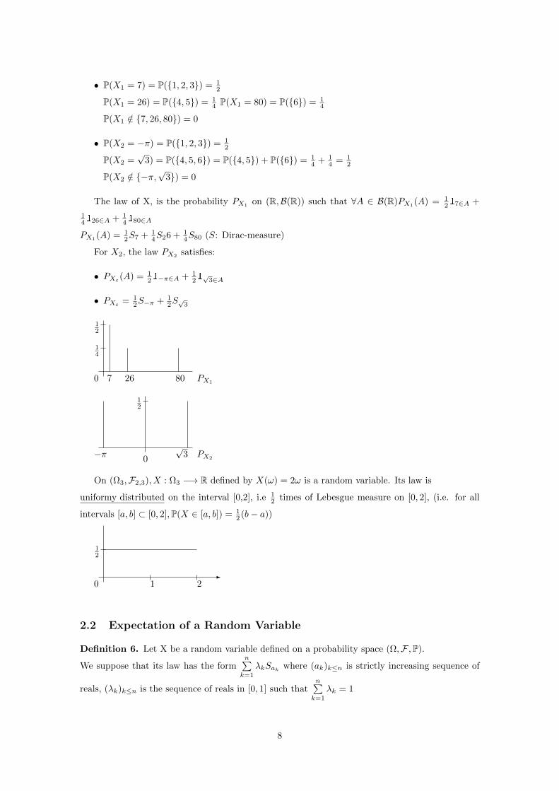
• P(X1 = 7) = P(1, 2, 3) = 12
P(X1 = 26) = P(4, 5) = 14 P(X1 = 80) = P(6) = 1
4
P(X1 /∈ 7, 26, 80) = 0
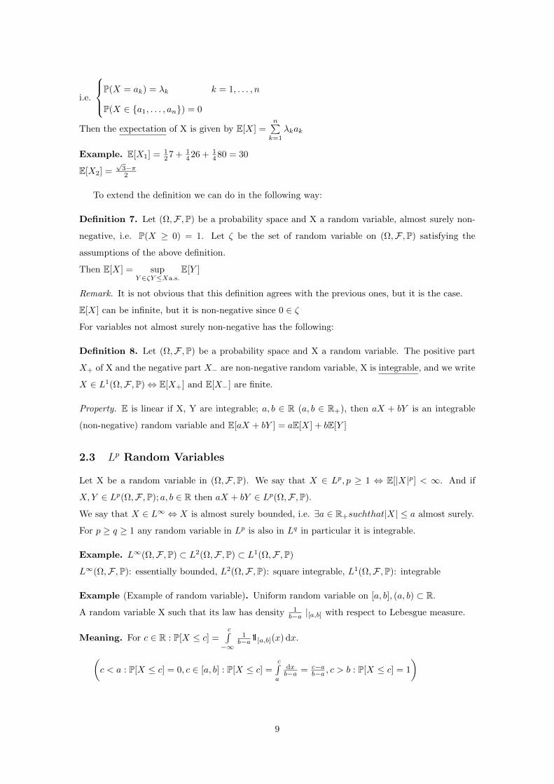
• P(X2 = −π) = P(1, 2, 3) = 12
P(X2 =√
3) = P(4, 5, 6) = P(4, 5) + P(6) = 14 + 1
4 = 12
P(X2 /∈ −π,√
3) = 0
The law of X, is the probability PX1on (R,B(R)) such that ∀A ∈ B(R)PX1
(A) = 1217∈A +
14126∈A + 1
4180∈A
PX1(A) = 1
2S7 + 14S26 + 1
4S80 (S: Dirac-measure)
For X2, the law PX2satisfies:
• PXε(A) = 121−π∈A + 1
21√3∈A
• PXε = 12S−π + 1
2S√3
0
12
14
PX17 26 80
0
12
PX2−π
√3
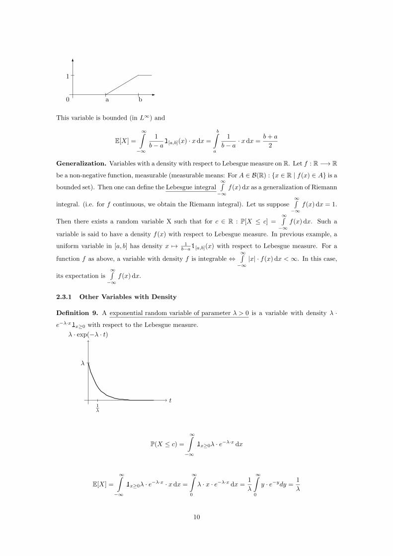
On (Ω3,F2,3), X : Ω3 −→ R defined by X(ω) = 2ω is a random variable. Its law is
uniformy distributed on the interval [0,2], i.e 12 times of Lebesgue measure on [0, 2], (i.e. for all
intervals [a, b] ⊂ [0, 2],P(X ∈ [a, b]) = 12 (b− a))
0-
12
1 2
2.2 Expectation of a Random Variable
Definition 6. Let X be a random variable defined on a probability space (Ω,F ,P).
We suppose that its law has the formn∑k=1
λkSak where (ak)k≤n is strictly increasing sequence of
reals, (λk)k≤n is the sequence of reals in [0, 1] such thatn∑k=1
λk = 1
8
i.e.
P(X = ak) = λk k = 1, . . . , n
P(X ∈ a1, . . . , an) = 0
Then the expectation of X is given by E[X] =n∑k=1
λkak
Example. E[X1] = 127 + 1
426 + 1480 = 30
E[X2] =√3−π2
To extend the definition we can do in the following way:
Definition 7. Let (Ω,F ,P) be a probability space and X a random variable, almost surely non-
negative, i.e. P(X ≥ 0) = 1. Let ζ be the set of random variable on (Ω,F ,P) satisfying the
assumptions of the above definition.
Then E[X] = supY ∈ζY≤Xa.s.
E[Y ]
Remark. It is not obvious that this definition agrees with the previous ones, but it is the case.
E[X] can be infinite, but it is non-negative since 0 ∈ ζ
For variables not almost surely non-negative has the following:
Definition 8. Let (Ω,F ,P) be a probability space and X a random variable. The positive part
X+ of X and the negative part X− are non-negative random variable, X is integrable, and we write
X ∈ L1(Ω,F ,P)⇔ E[X+] and E[X−] are finite.
Property. E is linear if X, Y are integrable; a, b ∈ R (a, b ∈ R+), then aX + bY is an integrable
(non-negative) random variable and E[aX + bY ] = aE[X] + bE[Y ]
2.3 Lp Random Variables
Let X be a random variable in (Ω,F ,P). We say that X ∈ Lp, p ≥ 1 ⇔ E[|X|p] < ∞. And if
X,Y ∈ Lp(Ω,F ,P); a, b ∈ R then aX + bY ∈ Lp(Ω,F ,P).
We say that X ∈ L∞ ⇔ X is almost surely bounded, i.e. ∃a ∈ R+suchthat|X| ≤ a almost surely.
For p ≥ q ≥ 1 any random variable in Lp is also in Lq in particular it is integrable.
Example. L∞(Ω,F ,P) ⊂ L2(Ω,F ,P) ⊂ L1(Ω,F ,P)
L∞(Ω,F ,P): essentially bounded, L2(Ω,F ,P): square integrable, L1(Ω,F ,P): integrable
Example (Example of random variable). Uniform random variable on [a, b], (a, b) ⊂ R.
A random variable X such that its law has density 1b−a |[a,b] with respect to Lebesgue measure.
Meaning. For c ∈ R : P[X ≤ c] =c∫−∞
1b−a1[a,b](x) dx.
(c < a : P[X ≤ c] = 0, c ∈ [a, b] : P[X ≤ c] =
c∫a
dxb−a = c−a
b−a , c > b : P[X ≤ c] = 1
)
9
0
6
-
1
"""""
a b
This variable is bounded (in L∞) and
E[X] =
∞∫−∞
1
b− a1[a,b](x) · xdx =
b∫a
1
b− a· xdx =
b+ a
2
Generalization. Variables with a density with respect to Lebesgue measure on R. Let f : R −→ R
be a non-negative function, measurable (measurable means: For A ∈ B(R) : x ∈ R | f(x) ∈ A is a
bounded set). Then one can define the Lebesgue integral∞∫−∞
f(x) dx as a generalization of Riemann
integral. (i.e. for f continuous, we obtain the Riemann integral). Let us suppose∞∫−∞
f(x) dx = 1.
Then there exists a random variable X such that for c ∈ R : P[X ≤ c] =∞∫−∞
f(x) dx. Such a
variable is said to have a density f(x) with respect to Lebesgue measure. In previous example, a
uniform variable in [a, b] has density x 7→ 1b−a1[a,b](x) with respect to Lebesgue measure. For a
function f as above, a variable with density f is integrable ⇔∞∫−∞|x| · f(x) dx <∞. In this case,
its expectation is∞∫−∞
f(x) dx.
2.3.1 Other Variables with Density
Definition 9. A exponential random variable of parameter λ > 0 is a variable with density λ ·
e−λ·x1x≥0 with respect to the Lebesgue measure.
t
λ · exp(−λ · t)
1λ
λ
P(X ≤ c) =
∞∫−∞
1x≥0λ · e−λ·x dx
E[X] =
∞∫−∞
1x≥0λ · e−λ·x · x dx =
∞∫0
λ · x · e−λ·x dx =1
λ
∞∫0
y · e−ydy =1
λ
10

where y = λ · x The variable is in Lp for all p ∈ [1,∞), because∞∫−∞
(1x≥0λ · e−λ·x
)|x|p dx < ∞,
but not for p =∞.
2.3.2 Gaussian (or Normal) Random Variable with Mean m ∈ R and Variance σ2 ∈ R∗+
Random variable with density: 1σ√2πexp
(−(x−m)2
2σ2
)This variable is not in L∞ but in all Lp for p ∈ [1,∞)(∞∫−∞
(1
σ√2πexp
(−(x−m)2
2σ2
))· |x|p dx <∞
)Expectation:
∞∫−∞
(1
σ√2πexp
(−(x−m)2
2σ2
))· x = m
Definition 10. Let X be a random variable on L2(Ω,F ,P). The variance of X is:
V ar(X) = E[(X − E[X])2] = E[X2]− (E[X])2 ≥ 0
Example. Variance of the previous Gaussian variable:
∞∫−∞
(1
σ√
2πexp
(−(x−m)2
2σ2
))· x2 dx−
∞∫−∞
(1
σ√
2πexp
(−(x−m)2
2σ2
))· x dx
which is equal to σ2
2.3.3 Example of Discrete Random Variable
(i.e. taking its values in a countable set (generally Z))
• Bernoulli random variable of parameter p ∈ [0, 1]:
Variable X such that P[X = 1] = p; P[X = 0] = 1− p (almost surely X ∈ 0, 1)
E[X] = p · 1 + (1− p) · 0 = p, E[X2] = p.
V ar(X) = p− p2 = p · (1− p)
• Symmetric Bernoulli random variable X such that:
P[X = 1] = P[X = −1] = 12 ; E[X] = 0; V ar(X) = 1
• Poisson random variable of parameters λ > 0:
It is a random variable X such that X ∈ N almost surely and for all n ∈ N : P([X = n]) =
e−λ · λn
n! .
We check that this problem exists, because
∞∑n=0
P[X = n] =
∞∑n=0
e−λ · λn
n!
= e−λ · eλ
= 1
11

E[X] =
∞∑n=0
(e−λ · λ
n
n!
)· n = λ
V ar(X) =
∞∑n=0
(e−λ · λ
n
n!
)· n2 − λ2 = λ
0
6
-λ = 31 2 3 4 5 6 7
3 Independence
Definition 11. Let (Ω,F ,P) be a probability space, G,H be two σ-algebra contained in F . G and
H are said to be independent :⇔ for all events A ∈ G, B ∈ H : P(A ∩B) = P(A) · P(B)
Example (modelling 2 successive coin flippers). F = P(Ω),
Ω = (H,H), (H,T ), (T,H), (T, T )
For all ω ∈ Ω : P(ω) = 14 (fair coins)
G is the σ-algebra generated by the first coordinate (first flipping), i.e. it contains the events
depending only on the first coordinates.
G = ∅, (H,H), (H,T ), (T ,H), (T , T ),Ω
H is the σ-algebra generated by the second coordinate.
G = ∅, H, (H), (T,H), (H,T ), (T, T ),Ω
It can be shown that G and H are independent.
Definition 12 (equivalent definition). Let (Ω,F ,P) be a probability space, (Gi)i∈I a family of
σ-algebras contained in F (finite or infinite). The two following statements are equivalent:
1. For all i1, . . . , in ∈ I distinct and for all events Ai1 ∈ Gi1 , · · ·Gin ∈ Gin : P(n⋂j=1
Aij ) =
n∏j=1
P(Aij ).
2. For all i1, . . . , in ∈ I distinct and for all random variables Xi1 , . . . , Xin bounded with Xij
measurable with respect to Gij , for all j ∈ 1 : n : E[n∏j=1
Xij ] =n∏j=1
E[Xij ]
If 1. or/and 2. are satisfied, we say that (Gi)i∈I are independent.
Definition 13 (Independence of random variables). Let (Ω,F ,P) be a probability space.
(Xi)i∈I is a family of random variables on this space. The variables (Xi)i∈I are independent if the
σ-algebra (Gi)i∈I are independent, where for all i ∈ I, Gi is the σ-algebra generated by the sets
ω ∈ Ω | Xi(ω) ∈ A, where A ∈ B(R).
12

Remark. Gi is the smallest σ-algebra such that Xi is a random variable with respect to the mea-
surable space (Ω,Gi). It is called the σ-algebra generated by Xi.
More generally, if (Xi)i∈I is a family of random variables, the σ-algebra generated by (Xi)i∈I is
the smallest σ-algebra κ such that Xi is a random variable on (Ω, κ) for all i ∈ I
Example. Let Ω = 0, 1N for some N ≥ 2, F = P(Ω), P is the uniform distribution on Ω(∀ω ∈ Ω : P(ω) = 2−N
). Then the random variables X1, . . . , XN are independent, where Xj(ω)
is the j-th coordinate of ω. This example is modelling N recursive coin flipping with a fair coin.
Proposition 1 (large families of independent random variables). Let
(Pi)i∈I be a family of probabilities on (R,B(R)). Then there exists (Xi)i∈I a family of independent
random variables such that Xi has distribution Pi, ∀i ∈ I.
For example one can construct (Xn)n≥1 independent and uniform on [0, 1] (on Gaussian, Pois-
son, exponential, ...).
Proposition 2 (law of large numbers). Let (Xn)n≥1 be a countable family of independent variables
with the same law (we say (Xn)n≥1 i.i.d.). Then, if X1 (or Xn for any n) is independent, then
almost surely: X1+···+XNN −→ E[X1]
Proposition 3 (central limit theorem). Let (Xn)n≥1 be a sequence of random variables on L2.
∆N := X1+···+XN−NE[X1]√N
converges in distribution to a Gaussian with expectation 0 and variance
σ2 = V ar(X1). (i.e. for a, v ∈ R, a < b : P(∆N ∈ (a, b)) −→ 1σ√2π
+b∫+a
e−x2/2π2
dx)
Example. If (Xn)n≥1 are i.i.d. random variables with law equal to Bernoulli distribution with
parameter 12 then X1+···+XN
N −→ 12 (N −→∞) a.s.
The difference of X1 + · · · + XN with its expectation value N2 is of order
√N , after dividing
by the order of the magnitude, the variables tends to a Gaussian random variable with variance
V ar(X1) = 1/4
3.1 Conditional Expectation
Definition 14. Let (Ω,F ,P) be a probability space and let X be a random variable on this space.
One suppose that either X ≥ 0 a.s. or X ∈ L1. For all σ-algebra G, included in F , there exists a
G-measurable random variable Y such that for all non-negative, bounded, G-measurable random
variable Z: E[XZ] = E[Y Z]. This variable Y is unique in the following sense: if Y1 and Y2 satisfy
this condition, then Y1 = Y2 a.s.
Y is called the conditional expectation of X with respect to G.
Definition 15. Let A be an event in F . The conditional probability of A with respect to G is the
conditional expectation of 1A with respect to G.
13
Definition 16. Let (Ti)i∈I be a family of random variables on (Ω, F ). The conditional expectation
of X with respect to (Ti)i∈I (resp. the conditional probability of A given (Ti)i∈I) is the conditional
expectation of X with respect to the σ-algebra generated by (Ti)i∈I (resp the conditional probability
of A with respect to the σ-algebra generated by (Ti)i∈I).
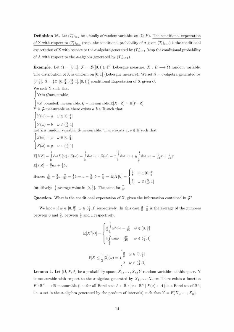
Example. Let Ω = [0, 1]; F = B([0, 1]); P: Lebesgue measure; X : Ω −→ Ω random variable.
The distribution of X is uniform on [0, 1] (Lebesgue measure). We set G = σ-algebra generated by
[0, 34 ]. G = ∅, [0, 34 ], ( 34 , 1], [0, 1] conditional Expectation of X given G.
We seek Y such thatY: is Gmeasurable
∀Z bounded, measurable, G −measurable,E[X · Z] = E[Y · Z]
Y is G-measurable ⇒ there exists a, b ∈ R such thatY (ω) = a ω ∈ [0, 34 ]
Y (ω) = b ω ∈ ( 34 , 1]
Let Z a random variable, G-measurable. There exists x, y ∈ R such thatZ(ω) = x ω ∈ [0, 34 ]
Z(ω) = y ω ∈ ( 34 , 1]
E[XZ] =1∫0
dωX(ω) · Z(ω) =1∫0
dω · ω · Z(ω) = x
34∫0
dω · ω + y1∫34
dω · ω = 932x+ 7
32y
E[Y Z] = 34ax+ 1
4by
Hence: 932 = 3
4a; 732 = 1
4b⇒ a = 38 ; b = 7
8 ⇒ E[X|G] =
38 ω ∈ [0, 34 ]
78 ω ∈ ( 3
4 , 1]
Intuitively: 38 average value in [0, 34 ]. The same for 7
8 .
Question. What is the conditional expectation of X, given the information contained in G?
We know if ω ∈ [0, 34 ], ω ∈ ( 34 , 1] respectively. In this case 3
8 , 78 is the average of the numbers
between 0 and 34 , between 3
4 and 1 respectively.
E[X2|G] =
43
34∫0
ω2dω = 316 ω ∈ [0, 34 ]
41∫34
ωdω = 3748 ω ∈ ( 3
4 , 1]
P[X ≤ 1
2|G](ω) =
23 ω ∈ [0, 34 ]
0 ω ∈ ( 34 , 1]
Lemma 4. Let (Ω,F ,P) be a probability space, X1, . . . , Xn, Y random variables at this space. Y
is measurable with respect to the σ-algebra generated by X1, . . . , Xn ⇔ There exists a function
F : Rn −→ R measurable (i.e. for all Borel sets A ⊂ R : x ∈ Rn | F (x) ∈ A is a Borel set of Rn,
i.e. a set in the σ-algebra generated by the product of intervals) such that Y = F (X1, . . . , Xn).
14
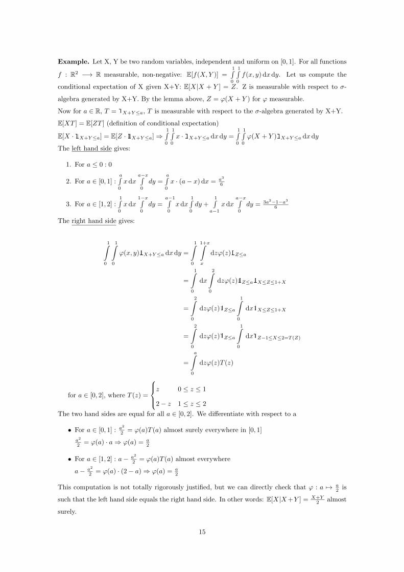
Example. Let X, Y be two random variables, independent and uniform on [0, 1]. For all functions
f : R2 −→ R measurable, non-negative: E[f(X,Y )] =1∫0
1∫0
f(x, y) dxdy. Let us compute the
conditional expectation of X given X+Y: E[X|X + Y ] = Z. Z is measurable with respect to σ-
algebra generated by X+Y. By the lemma above, Z = ϕ(X + Y ) for ϕ measurable.
Now for a ∈ R, T = 1X+Y≤a, T is measurable with respect to the σ-algebra generated by X+Y.
E[XT ] = E[ZT ] (definition of conditional expectation)
E[X · 1X+Y≤a] = E[Z · 1X+Y≤a]⇒1∫0
1∫0
x · 1X+Y≤a dx dy =1∫0
1∫0
ϕ(X + Y )1X+Y≤a dxdy
The left hand side gives:
1. For a ≤ 0 : 0
2. For a ∈ [0, 1] :a∫0
xdxa−x∫0
dy =a∫0
x · (a− x) dx = a3
6
3. For a ∈ [1, 2] :1∫0
xdx1−x∫0
dy =a−1∫0
xdx1∫0
dy +1∫
a−1xdx
a−x∫0
dy = 3a2−1−a36
The right hand side gives:
1∫0
1∫0
ϕ(x, y)1X+Y≤a dxdy =
1∫0
1+x∫x
dzϕ(z)1Z≤a
=
1∫0
dx
2∫0
dzϕ(z)1Z≤a1X≤Z≤1+X
=
2∫0
dzϕ(z)1Z≤a
1∫0
dx1X≤Z≤1+X
=
2∫0
dzϕ(z)1Z≤a
1∫0
dx1Z−1≤X≤2=T (Z)
=
a∫0
dzϕ(z)T (z)
for a ∈ [0, 2], where T (z) =
z 0 ≤ z ≤ 1
2− z 1 ≤ z ≤ 2
The two hand sides are equal for all a ∈ [0, 2]. We differentiate with respect to a
• For a ∈ [0, 1] : a2
2 = ϕ(a)T (a) almost surely everywhere in [0, 1]
a2
2 = ϕ(a) · a⇒ ϕ(a) = a2
• For a ∈ [1, 2] : a− a2
2 = ϕ(a)T (a) almost everywhere
a− a2
2 = ϕ(a) · (2− a)⇒ ϕ(a) = a2
This computation is not totally rigorously justified, but we can directly check that ϕ : a 7→ a2 is
such that the left hand side equals the right hand side. In other words: E[X|X+Y ] = X+Y2 almost
surely.
15

Property. conditional expectation:
1. For all σ-algebra G included F , and all almost surely non-negative random variable Y,
E[Y |G] ≥ 0 a.s.
2. For all G ⊂ F and all integrable random variable X, Y, all a, b ∈ R (a, b ∈ R+ resp.):
E[aX + bY |G] = aE[X|G] + bE[Y |G] almost surely
Example. In the last example:
E[X + Y |X + Y ] = aE[X|X + Y ] + E[Y |X + Y ].
It is obvious that E[X + Y |X + Y ] = X + Y almost surely.
By symmetry of the distribution of (X,Y): E[X|X + Y ] = E[Y |X + Y ]
⇒ X + Y = E[X + Y |X + Y ] = 2[X|X + Y ]⇒ E[X|X + Y ] = X+Y2
3. (Tower property): If κ ∈ G ⊂ F , X is non-negative or integrable.
E[E[X|G]|κ] = E[E[X|κ]|G] = E[X|κ]
In particular, since E[X|∅,Ω] = E[X]; E[E[X|G]] = E[X];
4. If X, Y are integrable and E[|XY |] <∞ and if Y is G-measurable then E[XY |G] = Y E[X|G]
5. If X and Y are independent, E[X|Y ] = E[X], if the σ-algebra generated by X and G are
independent then E[X|G] = E[X]
4 The Binomial Model
This is the most (non-trivial) simple financial model.
4.1 General Description
• The model is discrete. The price can only change at integers time: 1,...,T where T ≥ 1 is a
given integer. Trading is only possible at times 0,1,...,T.
• The model contains two securities: a bond, which is risk-less and corresponds to a ”certain
amount of money put into a bank account“, and a stock, which is risky, i.e. the price evolves
randomly.
• The price of the bond at time t is given by Bt = (1 + r)t, where r > −1 (generally r > 0) is
the interest rate corresponding to one unit of time.
• The price of the stock is fixed at time zero (S0), and satisfies the equation St = XtSt−1, for
all t ∈ 1, . . . , T, where Xt = 1 + u or Xt = 1 − d. Here u and d are fixed (they do not
depend on t), one has u+ d > 0 (i.e. 1 + u > 1− d) and generally, u > 0 and d > 0.
16

• The random variables (Xt)1≤t≤T are i.i.d. and for some p ∈ [0, 1] : P(Xt = 1 + u) = p;
P(Xt = 1− d) = 1− p
Example. T = 3, r = 0.05, u = 0.2, d = 0.2, p = 23 , S0 = 100
t = 0 t = 1 t = 2 t = 3
Bt : 1 1.05 1.1025 1.157825
172.8
144
23 hhhhhhhh
VVVVVVVV
120
23 iiiiiiii
UUUUUUUU 115.2
St : 100
23 jjjjjjj
13
TTTTTTTT 96
23 hhhhhhhhh
VVVVVVVVV
8023
iiiiiiiii
13
UUUUUUUUU 76.8
64
23 hhhhhhhhh
13
VVVVVVVVV
51.2
We need to construct explicitly the random variables (Xt)1≤t≤T
• The underlying measurable space is the set Ω = 1+u, 1−dT embedded with the σ-algebra.
F = P(Ω)
• The probability P put in the space is the probability measure satisfying P(ω) = pn(ω)(1−
p)T−n(ω), where n(ω) denotes the number of coordinates of ω which are equal to 1 + u.
• For all t ∈ 1, . . . , T the random variable Xt is the projection of coordinate number t, i.e.
Xt(ω1, . . . , ωT ) = ωt for all (ω1, . . . , ωT ) ∈ Ω. One can prove that the variables (Xt)t≤T are
i.i.d. random variables and satisfy P(Xt = 1 + u) = p, P(Xt = 1− d) = 1− p.
Example. (previous example) Ω = 1.2, 0.84, F = P(Ω) (216 sets)
– P((1.2; 1.2; 1.2; 1.2)) = p4 · (1− p)0 = p4 =(23
)4= 16
81
– P((0.8; 0.8; 0.8; 0.8)) = p0 · (1− p)4 =(13
)4= 1
81
– P((0.8; 1.2; 0.8; 1.2)) = P((0.8; 0.8; 1.2; 1.2)) = p2 · (1− p)2 =(23
)2 · ( 13)2 = 481
Moreover: Let L := ((0.8; 1.2; 0.8; 1.2)).
X1(L) = 0.8; X2(L) = 1.2; X3(L) = 0.8; X4(L) = 1.2;
Remark. To check that Xt has the ”good law“, we can write:
17

P(Xt = 1 + u) =∑
ω1,...,ωt−1,ωt+1,...,ωT
P((ω1, . . . , ωt−1, 1 + u, ωt+1, . . . , ωT ))
=∑
ω′∈1−d,1+uT−1
P((ω′1, . . . , ω′t−1, 1 + u, ω′t+1, . . . , ωT−1)), where ω′j =
ωj j < t
ωj − 1 j > t
=∑
ω′∈1−d,1+uT−1
pn((ω′1,...,ω′t−1,1+u,ω′t+1,...,ωT−1)) · (1− p)T−((ω′1,...,ω
′t−1,1+u,ω′t+1,...,ωT−1))
=∑
ω′∈1−d,1+u
pn(ω′)+1 · (1− p)T−1−n(ω′)
= p ·∑
ω′1,...,ω′T−1∈1−d,1+u
p
T−1∑j=1
1ω′j=1+u
· (1− p)T−1∑j=1
1ω′j=1−d
= p ·∑
ω′1,...,ω′T−1∈1−d,1+u
(T−1∏j=1
p1ω′j=1+u
)·
(T−1∏j=1
(1− p)1ω′j=1−d
)
= · · ·
= p ·T−1∏j=1
∑ω′∈1−d,1+u
p1ω′=1−d · (1− p)1ω′=1+u
= p
We omit the independence. Once the probability space (Ω,F ,P) is constructed we put into it a
family of σ-algebras, called a filtration.
Definition 17. Let (Ω,F ,P) be a probability space. A family (Ft)t∈I of σ-algebras, indexed by
a set I included in R+, is called a filtration ⇔ the following conditions hold:
• ∀t ∈ I: Ft is included in F .
• (Ft)t∈I is increasing with respect to t, i.e. if t, u ∈ I : t ≤ u⇒ Ft ⊆ Fu
The filtration put in the binomial model is indexed by the set I = 0, . . . , T, and it is defined as
follows: ∀t ∈ I : Ft = σ(X1, . . . , Xt). (σ-algebra generated by X1, . . . , Xt).
Example. In the situation above
• F0 = ∅,Ω (it is generated by ”nothing“)
• F1 = ∅, ω ∈ Ω | X1(ω) = 0.8, ω ∈ Ω | X1(ω) = 1.2,Ω
Contain the four sets ”depending only on the first coordinate“. (i.e. if A ∈ F1, and if
ω1, ω2 ∈ Ω have the same first coordinate, then they are either both in A or both in the
complement of A).
• F2 contains all the sets depending only on the two first coordinates. (i.e. if A ∈ F2, and if
18
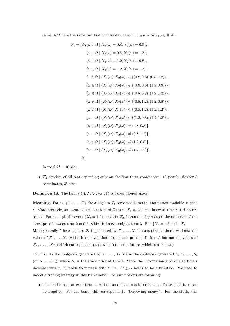
ω1, ω2 ∈ Ω have the same two first coordinates, then ω1, ω2 ∈ A or ω1, ω2 6∈ A).
F2 = ∅,ω ∈ Ω | X1(ω) = 0.8, X2(ω) = 0.8,
ω ∈ Ω | X1(ω) = 0.8, X2(ω) = 1.2,
ω ∈ Ω | X1(ω) = 1.2, X2(ω) = 0.8,
ω ∈ Ω | X1(ω) = 1.2, X2(ω) = 1.2,
ω ∈ Ω | (X1(ω), X2(ω)) ∈ (0.8, 0.8), (0.8, 1.2),
ω ∈ Ω | (X1(ω), X2(ω)) ∈ (0.8, 0.8), (1.2, 0.8),
ω ∈ Ω | (X1(ω), X2(ω)) ∈ (0.8, 0.8), (1.2, 1.2),
ω ∈ Ω | (X1(ω), X2(ω)) ∈ (0.8, 1.2), (1.2, 0.8),
ω ∈ Ω | (X1(ω), X2(ω)) ∈ (0.8, 1.2), (1.2, 1.2),
ω ∈ Ω | (X1(ω), X2(ω)) ∈ (1.2, 0.8), (1.2, 1.2),
ω ∈ Ω | (X1(ω), X2(ω)) 6= (0.8, 0.8),
ω ∈ Ω | (X1(ω), X2(ω)) 6= (0.8, 1.2),
ω ∈ Ω | (X1(ω), X2(ω)) 6= (1.2, 0.8),
ω ∈ Ω | (X1(ω), X2(ω)) 6= (1.2, 1.2),
Ω
In total 24 = 16 sets.
• F3 consists of all sets depending only on the first three coordinates. (8 possibilities for 3
coordinates, 38 sets)
Definition 18. The family (Ω,F , (Ft)t∈I ,P) is called filtered space.
Meaning. For t ∈ 0, 1, . . . , T the σ-algebra Ft corresponds to the information available at time
t. More precisely, an event A (i.e. a subset of Ω) is in Ft ⇔ one can know at time t if A occurs
or not. For example the event X3 = 1.2 is not in F2, because it depends on the evolution of the
stock price between time 2 and 3, which is known only at time 3. But X3 = 1.2 is in F3.
More generally ”the σ-algebra Ft is generated by X1, . . . , Xt“ means that at time t we know the
values of X1, . . . , Xt (which is the evolution of the stock price until time t) but not the values of
Xt+1, . . . , XT (which corresponds to the evolution in the future, which is unknown).
Remark. Ft the σ-algebra generated by X1, . . . , Xt is also the σ-algebra generated by S1, . . . , St
(or S0, . . . , St), where Si is the stock price at time i. Since the information available at time t
increases with t, Ft needs to increase with t, i.e. (Ft)t∈I needs to be a filtration. We need to
model a trading strategy in this framework. The assumptions are following:
• The trader has, at each time, a certain amount of stocks or bonds. These quantities can
be negative. For the bond, this corresponds to ”borrowing money“. For the stock, this
19
corresponds to ”short-selling“ (the trader ” sells sharers he doesn’t have“, he needs to buy
and then give them in the future).
• No trading is possible except at times 1, 2, . . . , T . The quantity of stocks and bonds hold is
constant in each of the intervals of the form (t − 1, t] for all t ∈ 1, 2, . . . T. The quantity
of bonds hold on the interval of time (t − 1, t] is αt, the quantity of stocks is βt. αt and βt
need to be determined only by using information available at time t− 1. This is why we can
consider the following definition:
Definition 19. A portfolio consists of two families (αt)t∈1,...,T and (βt)t∈1,...,T of random
variables, such that αt and βt are Ft−1 measurable for all t ∈ 1, . . . , T. αt (resp. βt) represents
the quantity of bonds (resp. stocks) hold in the interval of time (t− 1, t].
Remark. A portfolio is also called a trading strategy. It is not possible to follow all the trading
strategies, if there is no ”money coming from outside“. For example, if α1 = β1 = 0 (nothing hold
between times 0 and 1) one cannot have α2, β2 > 0 without earning money before time 1. (i.e.
one cannot obtain stocks and bonds for free). That is why we often restrict the possible portfolio
for which there is no ”extra money from outside“. The condition is the following: the value of the
portfolio does not change during the instants of trading. More precisely, for t ∈ 1, . . . , T − 1:
• The value of the portfolio at time t: αt ·Bt + βt · St
• Just after trading at time t, there are αt+1 bonds and βt+1 stocks in the portfolio and the
value is: αt+1 ·Bt + βt+1 · St. These two values has to be equal.
Note. Self-financial strategy corresponds to strategy with ”no money coming from outside“.
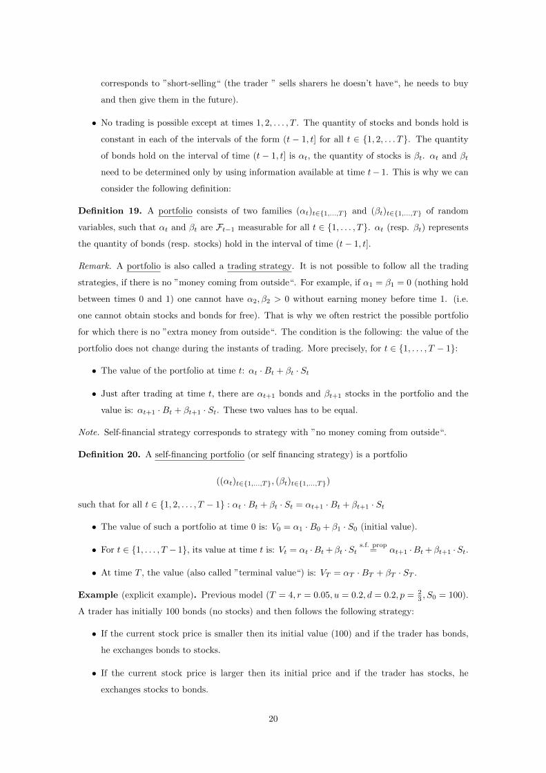
Definition 20. A self-financing portfolio (or self financing strategy) is a portfolio
((αt)t∈1,...,T, (βt)t∈1,...,T)
such that for all t ∈ 1, 2, . . . , T − 1 : αt ·Bt + βt · St = αt+1 ·Bt + βt+1 · St
• The value of such a portfolio at time 0 is: V0 = α1 ·B0 + β1 · S0 (initial value).
• For t ∈ 1, . . . , T − 1, its value at time t is: Vt = αt ·Bt +βt ·Sts.f. prop
= αt+1 ·Bt +βt+1 ·St.
• At time T , the value (also called ”terminal value“) is: VT = αT ·BT + βT · ST .
Example (explicit example). Previous model (T = 4, r = 0.05, u = 0.2, d = 0.2, p = 23 , S0 = 100).
A trader has initially 100 bonds (no stocks) and then follows the following strategy:
• If the current stock price is smaller then its initial value (100) and if the trader has bonds,
he exchanges bonds to stocks.
• If the current stock price is larger then its initial price and if the trader has stocks, he
exchanges stocks to bonds.
20

4.2 Description of the strategy
• α1 = 100, β1 = 0 (100 bonds at the beginning and 0 stocks).
• If X1 = 1.2 and then S1 = 120, the trader doesn’t buy stocks, and then α2 = 100, β2 = 0.
• If X1 = 0.8 and then S1 = 80, the trader buys stocks. He can buy a number of stocks equal
to V1
S1, where V1 is the value of portfolio at time 1, i.e. β2 = V1
S1= α1·B1
S1= 100·1.05
80 ≈ 1.3125
(in such a market, the number of stocks is an integer, but we don’t care about this problem).
⇒ α2 = 0, β2 ≈ 1.3125. (α2, β2) depends only on X1, α2, β2 are F1-measurable.
144
120
kkkkkk
SSSSSS
100
kkkkkk
SSSSSS 96
80
kkkkkkk
SSSSSSS
64
• If X1 = X2 = 1.2 then α3 = 100, β3 = 0.
• If X1 = 1.2, X2 = 0.8 then 96 = S2 < S1 = 100 ⇒ the trader buys stocks. The number of
stocks is β3 = V2
S2= α2·B2
S2= 100·(1.05)2
96 = 1.15 ⇒ α3 = 0, β3 ≈ 1.1484375.
• If X1 = 0.8, X2 = 1.2 (S1 = 80, S2 = 96) stocks are bought at time 1 and hold again after
time 2. α3 = 0, β3 ≈ 1.3125 (no change at time 2).
• If X1 = X2 = 0.8 the situation is similar: α3 = 0, β3 ≈ 1.3125.
• If X1 = X2 = 1.2 for any X3: α4 = 100, β4 = 0.
• If X1 = 1.2, X2 = 0.8, X3 = 1.2 stocks are bought at time 2 (S2 = 96) (α3 = 0, β3 = 1.15)
and sold at time 3. (S3 = 115.2) ⇒ β4 = 0, α4 = V3
B3= β3·S3
B3= 1.14·115.2
(1.05)3 ≈ 114.286.
• If X1 = 1.2, X2 = X3 = 0.8, α4 = 0, β4 = 1.15 (stocks bought at time 2).
• If X1 = 0.8, X2 = X3 = 1.2 the trader buy 1.3125 stocks at time 1 and sell at time 3,
α4 = 1.3125·115.2(1.05)3 ≈ 130.612.
• If X1 = 0.8, X2 or X3 = 0.8, stocks are bought at time 1, α4 = 0, β4 ≈ 1.3125.
Price evolution:
172.8
144
jjjjjj
TTTTTT
120
kkkkkk
SSSSSS 115.2
100
kkkkkk
SSSSSS 96
jjjjjj
TTTTTTT
80
kkkkkkk
SSSSSSS 76.8
64
jjjjjjj
TTTTTTT
51.2
21

The goal of the section is to maximize the terminal value V4 = α4 · Bt + β4 · S4. Value V4 in the
function of the stock price evolution:
1
1 1
V4 = 121.55 ⊕
1 PPPq
1
V4 = 138.92 ⊕1 PPPq PPPq
1
V4 = 105.84 1 PPPq PPPq PPPq V4 = 70.56
PPPq 1
1 1
V4 = 158.76 ⊕
PPPq 1 PPPq
1
V4 = 120.96
PPPq 1 PPPq PPPq V4 = 80.64
PPPq PPPq 1
1
V4 = 120.96 PPPq PPPq
1 PPPqV4 = 80.64
PPPq PPPq PPPq 1
V4 = 80.64 PPPq PPPq PPPq PPPq V4 = 53.76
The terminal value of the simples possible strategy: trading bonds. The terminal value
100 · (1.05)4 ≈ 121.55
22

⊕ : two strategies are equivalent
⊕: risky strategy is better
: save bonds
None of the two strategies is better than the other in any case. In particular, the ”risky strategy“
is not good if one pretends that it ”makes money“.
Imagine that if is possible to find a financial strategy that always gives more than what is obtained
by taking only bonds.
• Let (αt, βt)t∈1:T be this strategy and V0 its initial value.
• The strategy with only bonds, and with the same initial value contains V0/B0 = V0 bonds.
• The terminal value of the ”bond strategy“ is V0 ·BT .
• By assumption, the terminal value of the strategy (αt, βt)t∈1:T is VT > V0 ·BT .
• Let us consider the portfolio (αt − V0, βt)t∈1:T which is self-financing.
• The initial value is zero, and the terminal value is
(αT − V0)BT − Pt; St = VT − V0; BT > 0
That is why we state the following definition.
Definition 21. An arbitrage opportunity is a self-financing portfolio with initial value 0 and with
a terminal value non-negative and strictly positive with non zero probability.
Intuitive: An arbitrage opportunity corresponds to the possibility to earn money without taking
any risk. The existence of arbitrage opportunities is implied by the existence of strategies strictly
better than others (in any case).
In the real market the arbitrage opportunities tend to disappear.
The goal of this part of the chapter is to prove that in the binomial model satisfying 0 < 1− d <
1 + r < 1 +n, there does not exists an arbitrage opportunity. We also say that the binomial model
give a viable market.
Remark. One can check that if the conditions are not satisfied then there are arbitrage opportunity
(0 < 1 − d < 1 + r < 1 + n). The proof of viability of the binomial model involves the notion of
martingale.
Definition 22. Let (Ω,F , (Ft)t∈I ,Q) be a filtered probability space, and let (Xt)t∈I be a family
of integrable random variables such that Xt is Ft-measurable for all t ∈ I (here I is a subspace of
N).Then, (Xt)t∈I is a martingale (with respect to the space (Ω,F , (Ft)t∈I ,Q)⇔ for all s, t ∈ I, s ≤ t
one has: EQ[Xt|Fs] = Xs Q-a.s.
23

Remark. We denote the probability by Q (instead of P) because we need to deal with martingales
with respect to a probability, different from the initial probability of the model.
Note that the notion of martingale depends on the probability Q put into the space (Ω,F) (also
on the filtration (Ft)t∈I).
Example. Let (ζn)n≥1 be a family of i.i.d. and integrable random variable, and let Sn =n∑k=1
(ζk − E[ζk]). Then (Sn)n≥0 is a martingale with respect to the underlying probability space,
and the filtration (Fn)n≥0 such that for all n ≥ 0: Fn is the σ-algebra generated by the random
variables ζ1, . . . , ζn. Indeed for n ≥ 0:
E[Sn+1|Fn] = E[Sn|Fn] + E[ζn+1 − E[ζn+1]|Fn]
!= Sn + E[ζn+1 − E[ζn+1]]︸ ︷︷ ︸
E[ζn+1]−E[ζn+1]=0
= Sn
!: Sn is Fn-measurable and ζn+1 is independent of FnThen by tower property, for n > m we obtain:
E[Sn|Fm] = E[E[Sn|Fn−1]|Fm]
= E[Sn−1|Fm]
= E[E[Sn−1|Fn−2]|Fm]
= E[Sn−2|Fm]
= · · ·
= E[Sm|Fm]
= Sm
Note that, in this chapter, all the martingales corresponds to a filtration (Ft)t∈0:T indexed by
0 : T. In order to check that (Xt)t∈0:T is a martingale with respect to (Ω,F , (Ft)t∈0:T),Q)
we only need to check that EQ[Xt+1|Ft] = Xt, for t ∈ 0 : T −1 (by tower property of conditional
expectation).
In binomial model, we will transform the prices and change the probability measure, in order to
obtain martingales. Afterwards, we will deduce the non-existence of arbitrage opportunities.
• The bond price is deterministic and not constant in general (except if n = 0). The only
simple thing to do in order to transform it into a martingale is to change the ”unit taken for
measuring prices“, in order to make the bond price equal to one. In other words, the price
Bt of the bond is the now ”reference price“ for measuring all the amounts of money at time
t.
• That is why we consider the ”discounted stock price“. S∗t = StBt
which measures the stock
price as a quantity of bonds.
24

Example. (example stated above): (r = 0.05;u = 0.2; d = 0.2; p = 23 ;S0 = 100)
Bond price: Bt = (1 + r)t = (1.05)t at time t.
”Discounted stock price“:
S∗t =StBt
=St
(1 + r)t
t : t = 0 t = 1 t = 2
144(1.05)2
1201.05
23 mmmmmm
13
QQQQQQ
S∗t : 100
23 mmmmmmm
13
QQQQQQQ96
(1.05)2
801.05
23
mmmmmm
13
QQQQQQ
64(1.05)2
Unfortunately (S∗t )t∈0:T is not a martingale in general. Indeed, in this example:
E[S∗1 |F0] = E[S∗1 ] = 23 ·
1201.05 ·
13 ·
801.05 = 101.59 6= 100 = S∗0
One can also check that E[S∗2 |F1] 6= S∗1 .
In order to transform (S∗t )t∈0:T into a martingale, we will change the probability measure.
Recall that the prices (St)t∈0:T are constructed from the random variables (Xt)t∈1:T (St =
S0X1 · · ·Xt), which we defined as the coordinate function, from Ω = 1−d, 1+u to d−1, u+1
(i.e. Xt(ω) is the coordinate number t of ω).
The probability P on (Ω,F) = (Ω,P(Ω)) is defined by P(ω) = pn(ω)(1− p)T−n(ω) where n(ω) is
the number of coordinates equal to 1 + u in the T-tuple ω. In order to change the probability P,
we simply change the parameter p (a priori filed in the model) to a parameter q ∈ (0, 1) which, for
the moment, can be arbitrary chosen. This change of parameter allows us to define a probability
measure Q on (Ω, F ) satisfying Q(ω) = qn(ω)(1− q)T−n(ω).
Hence, we change the filtrated probability space (Ω,F , (Ft)t∈0:T,P), to the filtered probability
space (Ω,F , (Ft)t∈0:T,Q) the random variables X1, . . . , XT are not changed and we still consider
the stock prices St = S0X1 · · ·Xt and the discounted stock prices S∗t = St(1+r)t .
Under Q, the random variables (Xt)t∈0:T are still i.i.d. (as under P) but their law changes:
Q(Xt = 1 + u) = q; Q(Xt = 1− d) = 1− q (instead of P(Xt = 1 + u) = p; P(Xt = 1− d) = 1− p).
Remember that if p = q, then Q = P.
Definition 23. Let P and Q be two measures, defined on the same probability space. We say that
P is absolutely continuous with respect to Q :⇔ for all measurable sets A: Q(A) = 0 ⇒ P(A) = 0.
We say that P is equivalent to Q :⇔ P is absolutely continuous with respect to Q, and Q is
absolutely continuous with respect to P.
If P is equivalent to Q, P(A) = 0 ⇔ Q(A) = 0.
One has the following result:
25

Proposition 5. For any choice of the parameter q ∈ (0, 1) in the previous setting, Q is equivalent
to P.
Proof. : For any A of Ω, P(A) = 0⇔ Q(A) = 0⇔ A = ∅
Remark. In the binomial model, the situation is very simple and the rule of the notion of equivalent
measures is not so clear. However it is fundamental when we deal with more general financial
models.
Let us now go back to the stock prices considered as variables on the filtrated probability space
(Ω,F , (Ft)t∈I ,Q) and let us compute the conditional expectation of the discounted price S∗t+1,
given Ft for t ∈ 1, . . . , T.
One has:
EQ[S∗t+1|Ft] =EQ[St+1|Ft]
Bt+1
=EQ[St ·Xt|Ft]
Bt+1
=StBt+1
EQ[Xt+1|Ft]
=StBt
EQ[Xt+1]
=StBt+1
[q · (1 + u) + (1− q)(1− d)]
=St
(1 + r)t· q · (1 + u) + (1− q)(1− d)
1 + n
= S∗t
(q · (1 + u) + (1− q)(1− d)
1 + n
)Hence, (S∗t )t∈0:T is a martingale on (Ω,F , (Ft)t∈0:T,Q) ⇔ q(1+u)+(1−q)(1−d)
1+n = 1. Indeed if
q(1+u)+(1−q)(1−d)1+n 6= 1 one has EQ[S∗1 |F0] 6= S∗0 .
Let q(1+u)+(1−q)(1−d)1+n = 1 one has EQ[S∗t+1|Ft] ∀t ∈ 1, . . . , T.
q(1+u)+(1−q)(1−d)1+n = 1 ⇔ q = n+d
u+d . Since by assumption 0 < 1 − d < 1 + n < 1 + u, q is on the
interval (0, 1). It will be denoted by p∗, the associated probability measure is denoted by P∗ (i.e.
the measure Q for q = p∗) an it is called the risk-neutral probability measure.
Example. In the previous model, u = d = 0.2, n = 0.05 which implies p∗ = n+du+d = 0.05+0.2
0.2+0.2 = 58
(in particular p∗ 6= p = 23 ). Under P∗, the evolution of the stock price follows the picture:
144
120
58 kkkkkk
38
SSSSSS
100
58 kkkkkk
38
SSSSSS 96
8058
kkkkkkk
38
SSSSSSS
64
26

and for the discounted stock price:
144(1.05)2
1201.05
58 mmmmmm
38
QQQQQQ
100
58 oooooo
38
OOOOOO96
(1.05)2
801.05
58
mmmmmm
38
QQQQQQ
64(1.05)2
this discounted stock price is a martingale under P∗.
For example: EP∗[S∗1 |F0] = EP∗ [S
∗1 ] = 5
8 ·1201.05 + 3
8 ·801.05 = 840
8·1.05 = 100 = S∗0 .
Proposition 6. On the filtered probability space (Ω,F , (Ft)t∈0:T,P∗), the discounted stock
price (St)t∈0:T is a martingale. Moreover for any self-financing portfolio with value (Vt)t∈0:T
the discounted value (V ∗t := VtBt
)t∈0:T is a martingale.
Proof. We have proved that (S∗t )t≥0 is a martingale. Now, if (αt, βt)t∈0:T is a self-financing
portfolio, then for t ∈ 0 : T:
EP∗ [V∗t |Ft−1] =
EP∗ [Vt|Ft−1]
Bt
=EP∗ [αt ·Bt + βt · St|Ft−1]
Bt
= EP∗ [αt + βt · S∗t |Ft−1]
= αt + βtEP∗ [S∗t |Ft−1]
= αt + βt · S∗t−1
=αt ·Bt−1 + βt · St−1
Bt−1
=Vt−1Bt−1
= V ∗t−1
By tower property of conditional expectation: EP∗ [V∗t |Fs] = V ∗s for s ≤ t.
(V ∗t )t≥0 is a martingale.
Corollary 7. For any self-financing portfolio with initial value V0 and terminal value VT , one has:
EP∗ [Vt] = V0 · (1 + r)T
Proof. Since (V ∗t )t∈0:T is a martingale, one has:
EP∗ [Vt](Vt=V
∗t ·Bt)= Bt · EP∗ [V
∗T ]
(BT=(1+r)TF0 is trivial)= (1 + r)T · EP∗ [V
∗T |F0]
martingale property= (1 + r)TV ∗0
= V0(1 + r)T
27

This corollary can be interpreted as follows: If a trader starts with a given amount of money at
time 0, the expectation of the amount of money he has at time T , under risk-neutral probability
measure, does not depend on a strategy. It is equal to the value obtained with the risk-less strategy,
which consists of taking bonds from time 0 to time T .
From the corollary above, one can deduce that the market is viable.
Proposition 8. For any binomial model with parameters r, d, u satisfying 0 < 1−d < 1+r < 1+u
there does not exist an arbitrage opportunity.
Proof. Let us suppose that value of self-financing portfolio satisfies the conditions of an arbitrage
opportunity, i.e.:
• V0 = 0
• VT ≥ 0 P-almost surely, and P(VT > 0) > 0
Since P∗ is equivalent to P, one has P∗(VT > 0) > 0 and P∗(VT < 0) = 0 (recall that for any event
A, P(A) = 0 ⇔ P∗(A) = 0). Since P∗(VT < 0) = 0, VT ≥ 0, P∗-almost surely. Now P∗(VT ) > 0
and VT ≥ 0, P∗-almost surely, EP∗(VT ) > 0.
(P∗[VT > 0] > 0⇔ ∃ε > 0 : P∗[VT > ε] > 0
EP∗ [VT ] ≥ EP∗ [VT1VT>ε] ≥ EP∗ [ε · 1VT>ε] = ε · P∗[VT > ε] > 0)
On the other hand, EP∗ [VT ] = V0(1 + r)T = 0, which gives a contradiction.
Remark. Let us suppose that 0 < 1− d < 1 + u, but 1+r is not on the interval (1− d, 1 + u). One
can obtain an arbitrage opportunity.
• If 1 + r ≥ 1 + u, we consider a portfolio with β1 = −1 and α1 = S0 bonds (total value
at time 0: V0 = α1 · B0 + β1 · S0 = S0 · 1 + (−1) · S0 = 0). The terminal value is (if
there is no trading at times 1, 2, . . . , T − 1): VT = αt · BT + βt · ST = α1 · BT + β1 · ST =
S0(1 + r)T − 1 · S0 ·X1X2 · · ·XTno trading
= S0[(1 + r)T −X1 · · ·XT ]
• In any case, X1, X2, . . . , XT ≤ 1+u⇒X1·X2 · · ·XT ≤ (1+u)T , VT ≥ S0[(1+r)T−(1+u)T ] ≥
0
• If the stock price decreases all the time, (this event has strictly positive probability), VT =
S0[(1 + r)T − (1− d)T ] > 0. We have an arbitrage opportunity.
• If 1 + r ≤ 1− d, one obtain an arbitrage opportunity by taking 1 stock and −S0 bonds.
Intuitively:
• If 1 + r ≥ 1 + u, it is always better to hold bonds than stocks.
• If 1 + r ≤ 1− d, it is always better to hold stocks than bonds. Hence, it is natural to expect
that the market is not viable in this case.
28

At this point, we will be able to study the price of a certain kind of option, called European contin-
gent claims. Intuitively, these options give a certain amount of money at terminal time T (this
amount of money is called ”payoff“) depending on the evolution of the stock price.
Definition 24. A European contingent claim is an F = FT -measurable random variable (defined
on the set Ω), modelling the payoff of an option at time T .
Example.
• A constant function from Ω to R corresponding to a fixed payoff at time T .
• The terminal stock price ST .
• A call (resp. put) option with maturity T and stock price K, giving a payoff equal to
(ST −K)+ (resp. (ST −K)−).
• An option which gives 100 if the stock prices always increases and 0 otherwise. It corresponds
to a function equal to 100 at (1 + u, 1 + u, . . . , 1 + u) ∈ 1 − d, 1 + uT = Ω and 0 at any
other point.
Question (Fundamental problem). What is the ”fair price“ of an option? In other words, which
amount of money should I pay at time 0, for the right to buy the stock at price K, at time T (for
the call option)?
• For the first example a constant payoff c corresponds, at time T , to the price of CBT
=
c · (1 + r)−T bonds. The option is equivalent to c · (1 + r)−T bonds and then its fair price is
the initial value of these bonds, i.e. c · (1 + r)−T .
• For the second example, the payoff in the value of the stock, we can expect, at time 0, a fair
price equal to S0.
• The example of the call option is more difficult. Let us deal with a very simple particular
case:
Parameters: T = 1, S0 = 100, r = 0.01, u = 0.2, d = 0.1,K = 100, p ∈ (0, 1) arbitrary chosen.
The possible evolution of the prices is given by:
t = 0 t = 1
Bt : 1 1.1
120
St : 100
p jjjjjjj
1−p TTTTTTTT
90
29
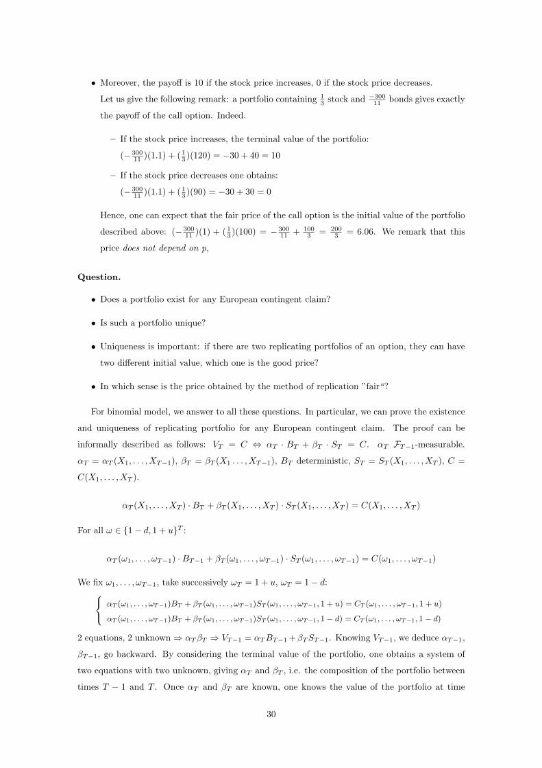
• Moreover, the payoff is 10 if the stock price increases, 0 if the stock price decreases.
Let us give the following remark: a portfolio containing 13 stock and −30011 bonds gives exactly
the payoff of the call option. Indeed.
– If the stock price increases, the terminal value of the portfolio:
(− 30011 )(1.1) + ( 1
3 )(120) = −30 + 40 = 10
– If the stock price decreases one obtains:
(− 30011 )(1.1) + ( 1
3 )(90) = −30 + 30 = 0
Hence, one can expect that the fair price of the call option is the initial value of the portfolio
described above: (− 30011 )(1) + (1
3 )(100) = − 30011 + 100
3 = 2003 = 6.06. We remark that this
price does not depend on p,
Question.
• Does a portfolio exist for any European contingent claim?
• Is such a portfolio unique?
• Uniqueness is important: if there are two replicating portfolios of an option, they can have
two different initial value, which one is the good price?
• In which sense is the price obtained by the method of replication ”fair“?
For binomial model, we answer to all these questions. In particular, we can prove the existence
and uniqueness of replicating portfolio for any European contingent claim. The proof can be
informally described as follows: VT = C ⇔ αT · BT + βT · ST = C. αT FT−1-measurable.
αT = αT (X1, . . . , XT−1), βT = βT (X1 . . . , XT−1), BT deterministic, ST = ST (X1, . . . , XT ), C =
C(X1, . . . , XT ).
αT (X1, . . . , XT ) ·BT + βT (X1, . . . , XT ) · ST (X1, . . . , XT ) = C(X1, . . . , XT )
For all ω ∈ 1− d, 1 + uT :
αT (ω1, . . . , ωT−1) ·BT−1 + βT (ω1, . . . , ωT−1) · ST (ω1, . . . , ωT−1) = C(ω1, . . . , ωT−1)
We fix ω1, . . . , ωT−1, take successively ωT = 1 + u, ωT = 1− d: αT (ω1, . . . , ωT−1)BT + βT (ω1, . . . , ωT−1)ST (ω1, . . . , ωT−1, 1 + u) = CT (ω1, . . . , ωT−1, 1 + u)
αT (ω1, . . . , ωT−1)BT + βT (ω1, . . . , ωT−1)ST (ω1, . . . , ωT−1, 1− d) = CT (ω1, . . . , ωT−1, 1− d)
2 equations, 2 unknown⇒ αTβT ⇒ VT−1 = αTBT−1 +βTST−1. Knowing VT−1, we deduce αT−1,
βT−1, go backward. By considering the terminal value of the portfolio, one obtains a system of
two equations with two unknown, giving αT and βT , i.e. the composition of the portfolio between
times T − 1 and T . Once αT and βT are known, one knows the value of the portfolio at time
30
T − 1, and by solving again a system of equations, one deduces αT−1 and βT−1. Then, we obtain
αT−2, βT−2, and we go backwards with α, β. The price statement is the following:
Proposition 9. Let us consider a binomial model with 0 < 1− d < 1 + r < 1 + u, with terminal
time T . Let CT be an European contingent claim. Then, for all t ∈ 1 : T, there exists a unique
family (αu, βu)u∈t,t+1,...,T, such that:
• For all u ∈ t, t+ 1, . . . , T, αu and βu are Fu−1-measurable random variables
• For all u ∈ t, t+ 1, . . . , T, αuBn + βuSn = αu+1Bn + βu+1Sn
• αTBT + βTST = CT (everywhere) ((αu, βu)u∈t,t+1,...,T can be considered as a portfolio
defined only after time t− 1)
Proof. By backward induction (from t = t, r = 1)
Let us first suppose t = T . One needs to find αT and βT FT−1-measurable, such that αTBT +
βTST = CT .
Since αT and βT are FT−1-measurable, they can be written as functions of (X1, . . . , XT−1), i.e.
αT = αT (X1, . . . , XT−1), βT = βT (X1, . . . , XT−1). The payoff CT , FT -measurable, can be written
as: CT (X1, . . . , XT−1). The equation becomes.
αT (X1, . . . , XT−1)(1 + r)T + βT (X1, . . . , XT−1)
So X1, . . . , XT = CT (X1, . . . , XT ).
For (ω1, . . . , ωT−1) ∈ 1 − d, 1 + uT−1 fixed, one deduces (by considering successively the cases
where X1 = ω1, . . . , XT−1 = ωT−1, XT = 1− d, and X1 = ω1, . . . , XT−1 = ωT−1, XT = 1 + u
(S)
αT (ω1, . . . , ωT−1)(1 + r)T + βT (ω1, . . . , ωT−1)S0ω1 · · ·ωT−1(1− d) = CT (ω1, . . . , ωT−1, 1− d)
αT (ω1, . . . , ωT−1)(1 + r)T + βT (ω1, . . . , ωT−1)S0ω1 · · ·ωT−1(1 + u) = CT (ω1, . . . , ωT−1, 1 + u)
Conversely, if the system (S) is satisfied for all (ω1, . . . , ωT−1) ∈ 1 − d, 1 + uT−1, the vari-
ables αT (X1, . . . , XT−1) and βT (X1, . . . , XT−1) satisfy the conditions given in the proposition.
Now, for all (ω1, . . . , ωT−1) ∈ 1 − d, 1 + uT−1, (S) has a unique solution (αT (ω1, . . . , ωT−1),
βT (ω1, . . . , ωT−1)), since its determinant:
det
(1 + r)T S0ω1 · · ·ωT−1(1− d)
(1 + r)T S0ω1 · · ·ωT−1(1 + u)
= (1 + r)TS0ω1 · · ·ωT−1(d+ u) 6= 0
This implies the proposition for t = T . Let us now suppose the proposition is true for t =
v ∈ 2, . . . , T, and let us prove it for t = v − 1. The conditions which need to be satisfied by
(αu, βu)u∈v−1,...,T are:
a) the same conditions as for t = v, concerning the variables (αu, βu)u∈v,...,T.
b) αu−1, βu−1 needs to be Fv−2-measurable.
31

c) Once (αu, βu)u∈v,...,T are given, one needs to have αv−1Bv−1 + βv−1Sv−1 = αvBv−1 +
βvSv−1.
The condition a) determines uniquely (αu, βu)u∈v,...,T since the proposition is supposed be sat-
isfied for t = v.
The condition b) implies that one can write
αv−1 = αv−1(X1, . . . , Xv−2) βv−1 = βv−1(X1, . . . , Xv−2)
(deterministic if r = 2)
The condition c) is satisfied iff for all (ω1, . . . , ωv−2) ∈ 1− d, 1 + uv−2
(S′)
αv−1(ω1, . . . , ωv−2)(1 + r)v−1 + βv−1(ω1, . . . , ωv−2)S0ω1 · · ·ωv−2(1 + u)
= αv(ω1, . . . , ωv−2, 1 + u)(1 + r)v−1 + βv(ω1, . . . , ωv−2, 1 + u)S0ω1 · · ·ωv−2 · (1 + u)
αv−1(ω1, . . . , ωv−2)(1 + r)v−1 + βv−1(ω1, . . . , ωv−2)S0ω1 · · ·ωv−2(1− d)
= αv(ω1, . . . , ωv−2, 1− d)(1 + r)v−1 + βv(ω1, . . . , ωv−2, 1− d)S0ω1 · · ·ωv−2 · (1− d)
Here αv(ω1, . . . , ωv−2, 1 + u), βv(ω1, . . . , ωv−2, 1 + u) are fixed, (similar with (1-d)) the unknown
variables are αv−1(ω1, . . . , ωv−2) and βv−1(ω1, . . . , ωv−2)
Hence, the system (S′) is a system of two equations with two unknown, with determinant
det
(1 + r)v−1 S0ω1 · · ·ωv−2(1 + u)
(1 + r)v−1 S0ω1 · · ·ωv−2(1− d)
6= 0
Therefore the system (S′) has a unique solution for all (ω1, . . . , ωv−2) ∈ 1− d, 1 + uv−2 and the
proposition is satisfied for t = v − 1
By backward induction we are done.
Corollary 10. In the binomial model 0 < 1− d < 1 + r < 1 + u any European contingent claim
admits a unique replicating portfolio.
Proof. This is an immediate consequence of the proposition above, applied for t = 1.
This existence and uniqueness of a replicating portfolio gives fair price for any European contingent
claim. However, solving all the equations should be complicated and one can expect a more
practical way to give this fair price.
One has the following (for a binomial model with 0 < 1− d < 1 + r < 1 + u):
Proposition 11. The initial value of the replicating portfolio of a European contingent claim CT
is given by V0 = E∗[CT ]BT
. In here E∗ denotes the expectation under the risk-neutral probability
measure. Moreover, for all t ∈ 0, 1, . . . , T its value is E∗[CT |Ft]( BtBT ) = Vt
Proof. As shown before, under risk-neutral probability measure, the discounted value (V ∗t )t∈0:T
of the portfolio is a martingale. Now, by assumption, one has VT = CT and then V ∗T = CTBT
. Hence,
by martingale property V ∗t = E∗[V ∗T |Ft] = E∗[Ct|Ft]Bt
and Vt = BtV∗t = E∗[CT |Ft]( BtBT ). For t = 0,
we obtain the fair price of the option: V0 = E∗[CT |F0] B0
BT= E∗[CT ]
BT.
32

4.3 Price of the European Contingent Claim
Expectation under the risk-neutral probability measure: E∗[CT ]BT
Value of the replicating portfolio at time t: E∗[CT |Ft] ·(BtBT
)Example (call option). T = 1, S0 = 100, r = 0.1, u = 0.2, d = 0.1, CT = (ST − 110)+ (call option
with strike price 110). Following evolution of prices:
t : t = 0 t = 1
Bt : 1 1.1
120
St : 100
p jjjjjjj
1−p TTTTTTTT
80
In this example, the replicating portfolio was constructed by hand ( 20033 = 6.06)
Let us compute it as an expectation with respect to the risk-neutral measure. The parameter p
corresponding to the risk-neutral measure is p∗ = r+du+d ⇒ p∗ = 0.2
0.3 = 23 . Hence, one can compute
the ”fair price“ of the call option as follows:
E∗[(ST − 110)+]
BT=
[ 23 (120− 110)+ + 13 (90− 110)+]
1.1
=[ 2310 + 1
30]
1.1
=
(20
3
)·(
1
1.1
)=
200
33
= 6.06
the same value as computed above.
A more difficult example is the first example given in this chapter (S0 = 100, T = 4, r = 0.05, u =
d = 0.2, p = 23 ) with a call option with strike price K = 100. Recall that the risk-natural measure
corresponds to: p∗ = r+du+d = 0.25
0.4 = 58 . Hence, the fair price of the option is:
E∗[(ST−100)+]BT
= (207.36−100)+·π4+(1328.24−100)+·π3+(92.16−100)+·π2+(61.44−100)+·π1+(40.96−100)+·π0
(1.05)4 ,
where
π4 = P∗[S4 = 207.36], . . . , π0 = P∗[S4 = 40.96]
π4 = ( 58 )4 = 625
4096 (the price has to increase 4 times)
π3 =(41
)· ( 5
8 )3 · ( 38 ) = 4 · ( 5
8 )3 · ( 38 ) = 1500
4096 (the price has to increase 4 times and decrease 1 time)
π2 =(42
)· ( 5
8 )2 · ( 38 )2 = 6 · ( 5
8 )2 · ( 38 )2 = 1350
4096
π1 = 4 · ( 58 ) · ( 3
8 )3 = 5404096
π0 = ( 38 )4 = 81
4096
Price of the call option:(107.36)·( 625
4096 )+(38.24)·( 15004096 )+0+0+0
(1.05)4 = 25
Let us compute the value of the portfolio of the replicating portfolio at time 1,2,3,4; if we
suppose that the stock price increases, decreases, increases and increases again (i.e. S0 = 100, S1 =
33

120, S2 = 96, S3 = 115.2, S4 = 138.24) (beginning: price of the option = 25, end : payoff = 38.24
for this scenario)
• The initial value of the portfolio is close to 25.
• The value at time 1 is E∗[(S4 − 100)+|F1] · (B1
B4). Conditionally on this event (S1 = 120)
which corresponds to the informations available at time 1.
– The price increases 3 times from time 1 to time 4 with probability ( 58 )3. The terminal
price is S4 = 207.36
– The price increases twice and decreases once. Probability: 3 · ( 58 )2 · ( 3
8 ). Terminal price:
S4 = 138.24
– The price decreases twice and increases once. Probability: 3 · ( 58 ) · ( 3
8 )2. Terminal price:
S4 = 92.16
– The price decreases 3 times. Probability: ( 58 )3. Terminal price: S4 = 61.44
For S1 = 120, the price of the portfolio at time 1 is:
E∗[(S4 − 100)+|F1] · (B1
B4)
= [1
(1.05)3] · [( 5
8)3 · (207.36− 100)++
3 · (58)3 · (3
8) · (138.24− 100)+ + 3 · (3
8)2 · (5
8) · (92.16− 100)+ + (
3
8)3 · (61.44− 100)+]
= 37.16 = V1.
One can compute V1 for the scenario S1 = 80, and it gives a different result.
• The value V2 at time 2 is E∗[(S4 − 100)+|F2] · (B2
B4). Conditionally on S1 = 120, S2 = 96, 3
possibilities can hold.
– The price increases twice from time 2 to time 4. Probability: ( 58 )2, S4 = 138.24
– The price increases once and decreases once. Probability: 2 · 58 ·38 , S4 = 92.16
– The price decreases twice. Probability: ( 38 )2, S2 = 61.44
Hence for S1 = 120, S2 = 96 V2 = ( 1(1.05)2 ) · [( 5
8 )2 · (138.24−100)+ +2 · ( 58 ) · ( 3
8 ) · (92.16−
100)+ + ( 38 )2 · (61.44− 100)+] = 13.55.
• The value V3 at time 3 is E∗[(S4 − 100)+|F3] · (B3
B4)
For S1 = 120, S2 = 96, S3 = 115.2, one has conditionally on F3
– S4 = 138.24 with probability 58
– S4 = 92.16 with probability 38
V3 = ( 58 · (138.24− 100)+ + 3
8 · (92.16− 100)+) · 11.05 = 22.76
• Value at time 4, V4 is equal to the payoff. In the scenario S1 = 120, S2 = 96, S3 = 115.2,
S4 = 138.24. V4 = (S4 − 100)+ = 38.24.
34

At each step, we compute the value of any replicating portfolio at any time. However, for a
trader who follows the corresponding strategy, it is also important to know the composition of the
portfolio at any time and not only its value. Of course, one can solve explicitly the corresponding
system of equations given above (proof of existence uniqueness of the replicating portfolio) but it
is not very practical. In fact, the following proposition gives an explicit form of its solution.
Proposition 12. Let (αt, βt)t∈1:T be the replicating portfolio of a European contingent claim
CT . Then for all t, αt and βt are explicitly given by:
(∗)
αt =
V(d)t S
(u)t −V
(u)t ·S(d)
t
Bt(S(u)t −S
(d)t )
βt =V
(u)t −V (d)
t
S(u)t −S
(d)t
where V(d)t (respectively V
(u)t , S
(d)t , S
(u)t ) is the Ft−1-measurable random variable equal to
Vt(ω1, . . . , ωt−1, 1− d)
(respectively Vt(ω1, . . . , ωt−1, 1 + u), St(ω1, . . . , ωt−1, 1 + u)) on the event
X1 = ω1, . . . , Xt−1 = ωt−1,
where Vt(ω1, . . . , ωt) denotes the value of the replicating portfolio of CT for X1 = ω1, . . . , Xt = ωt
(respectively St(ω1, . . . , ωt) is the value of the stock price for X1 = ω1, . . . , Xt = ωt).
Example. S(u)t = St−1︸︷︷︸
evolution of Swith time t− 1
· (1− u)︸ ︷︷ ︸assumption:
the price increasesbetween time t− 1 and t
,
S(d)t = St−1 · (1− d), S
(u)t − S(d)
t = St−1 · (u+ d)
Proof. Let us define αt and βt by the equality (∗) and let us prove the (αt, βt)t∈1:T replicates
CT . Since V(d)t , V
(u)t , S
(d)t , S
(u)t depend only on X1, . . . , Xt−1 they are Ft−1-measurable and hence
(αt, βt)t∈1:T defines a portfolio.
We need to prove that it is self-financing, and to check its terminal value.
Self-financing property: For t ∈ 1, . . . , T one has:
αt ·Bt + βt · St =V
(d)t · S(u)
t − V (u)t · S(d)
t
S(u)t − S(d)
t
+V
(u)t − V (d)
t
S(u)t − S(d)
t
· St
• If Xt = 1 + u (i.e. the stock price is multiplied by 1 + u from time t− 1 to t) then St = S(u)t
αt ·Bt + βt · St =V
(d)t ·S(u)
t −V(u)t ·S(d)
t
S(u)t −S
(d)t
+V
(u)t −V (d)
t
S(u)t −S
(d)t
· S(u)t = V
(u)t .
• If Xt = 1− d: αt ·Bt + βt · St =V
(d)t ·S(u)
t −V(u)t ·S(d)
t
S(u)t −S
(d)t
+V
(u)t −V (d)
t
S(u)t −S
(d)t
· S(d)t︸︷︷︸St
= V(d)t
Hence, in any case αt ·Bt + βt · St = Vt (= EP∗ [CT |FT ]( BtBT ))
• For t ∈ 0, . . . , T−1 one also has: αt+1 ·Bt+βt+1 ·St =V
(d)t+1·S
(u)t+1−V
(u)t+1·S
(d)t+1
Bt+1(S(u)t+1−S
(d)t+1)
·Bt+V
(u)t+1−V
(d)t+1
S(u)t+1−S
(d)t+1
·St.
If Xt+1 = 1 + u: St+1 = (1 + u) · St. Hence, S(u)t+1 = (1 + u) · St.
35

• Similarly S(d)t+1 = St · (1− d). Bt
Bt+1= 1
(1+r) .
αt+1 ·Bt + βt+1 · St =V
(d)t+1·St(1+u)−V
(u)t+1·St(1−d)
St(u+s)(1+r)+
V(u)t+1−V
(d)t+1
u+d
=V
(d)t+1(1+u)−V
(u)t+1(1−d)+(1+r)(V
(u)t+1−V
(d)t+1)
(1+r)(u+d) =(u−r)V (d)
t+1+V(u)t+1(r+d)
(1+r)(u+d)
p∗= r+du+d
= 11+r
[V
(d)t+1 · (1− p∗) + V
(u)t+1 · p∗
]!= 1
1+rE[Vt+1|Ft] = Vt
since Vt+1 = Bt+1
BTE∗[CT |Ft+1],
Vt = BtBT
E∗[CT |Ft+1] ( VtBt is a martingale)
Therefore: For t ∈ 1, . . . , T − 1: αt · Bt + βt · St = αt+1 · Bt + βt+1 · St = Vt. The portfolio is
self-financing.
Moreover, its terminal value is: αT · BT + βT · ST = VT and VT = CT (since VT is the terminal
value of the replicating portfolio of CT ).
One deduces that (αt, βt)t∈1:T replicates the contingent claim CT . By uniqueness we are done
Example. As last time T = 4, S0 = 100, r = 0.05, u = d = 0.2, p = 23 . Let us suppose that the
scenario S0 = 100, S1 = 120, S2 = 96, S3 = 115.2, S4 = 138.24 happens. Let us replicate the call
option with strike price 100.
• V (u)1 = V1|X1=1+u = E∗[(S4 − 100)t|F1]|X1=1+u ·
(B1
B4
)= E∗[(S4 − 100)t|X1 = 1 + u] ·
(B1
B4
)Now conditionally on X1 = 1 + u
• The price can increase 3-times from 1 to 4. Conditional probability: (p∗)3
=(58
)3. In this
case S4 = 207.36.
• The price can also increase twice and decrease once. Conditional probability: 3 ·(38
)·(58
)2.
In this case S4 = 138.24.
• The price can decrease twice and increase once. Conditional probability: 3 ·(38
)2 · ( 58). In
this case S4 = 92.16.
• The price can decrease 3-times. Conditional probability:(38
)3. In this case S4 = 61.44.
Hence:
V(u)1 =
[( 58 )3 · 107.36 + 3 · ( 5
8 )2 · ( 38 ) · 38.24 + 0 + 0
](1.05)3
⇒ V(u)1 = 37.16
Similarly, V(d)1 = EP∗ [(S4 − 100)t|X1 = 1− d](B1
B4).
The different scenario are same as for V(u)1 , except that S4 is ”down-shifted“
207.36 → 138.24
138.24 → 92.16
92.16 → 61.44
61.44 → 40.96
36

One deduces
V(d)1 =
[( 58 )3 · 38.24 + 0 + 0 + 0]
(1.05)3≈ 8.065
One has by supporting S1 = 120 (and then X1 = 1.2): V(u)2 = V2|X2=1+u=1.2 = V2|X1=X2=1.2 =
EP∗ [(S4 − 100)t|F2]|X1=X2=1.2 · (B2
B4) = E∗[(S4 − 100)t|X1 = X2 = 1.2].
Conditionally on X+ = X2 = 1.2
• The price can increase twice after time 2: Conditional probability: ( 58 )2 S4 ≈ 207.36.
• The price can increase once and decrease once: Conditional probability: 2 · ( 38 ) · ( 5
8 ) S4 ≈
138.24.
• The price can decrease twice: Conditional probability: ( 38 )2 S4 ≈ 92.16.
Hence: V(u)2 =
[( 58 )
2(107.36)+2·( 58 )(
38 )(38.24)+0]
(1.05)2 = 54.3.
Similarly: V(d)2 = E∗[(S4 − 100)t|X1 = 1.2, X2 = 0.8] =
[( 58 )
2(38.24)+0+0]
(1.05)2 = 13.55.
In the scenario S1 = 120, S2 = 96 (X1 = 1.2, X2 = 0.8).
One obtains: V(u)3 = E∗[(S4 − 100)t|X1 = 1.2, X2 = 0.8, X3 = 1.2] · (B3
B4).
Conditionally on X1 = 1.2, X2 = 0.8, X3 = 1.2:
• S can increase from time 3 to time 4. Probability: 58 , S4 = 138.24.
• S can decrease from time 3 to time 4. Probability: 38 , S4 = 92.16.
V(u)3 =
[( 58 )(38.24)+0]
1.05 = 22.76
Similarly: V(u)3 = E∗[(S4 − 100)t|X1 = 1.2, X2 = 0.8, X3 = 0.8] = 0.
For the scenario S1 = 120, S2 = 96, S3 = 115.2 (X1 = 1.2, X2 = 0.8, X3 = 1.2) one has:
V(u)4 = (S4 − 100)t|X1 = 1.2, X2 = 0.8, X3 = 1.2, X4 = 1.2 = (138.24− 100)t = 38.24.
V(d)4 = (S4 − 100)t|X1 = 1.2, X2 = 0.8, X3 = 1.2, X4 = 0.8 = 0.
We remark that in the scenario above V(u)1 = V1, V
(d)2 = V2, V
(u)3 = V3 since X1 = 1.2 = 1 + u,
X2 = 0.8 = 1− d, X3 = 1.2 = 1 + u.
Since, X4 in the scenario is supposed to be 1 + u, X(u)4 = V4 corresponds to the payoff of the
option.
For this values, one deduces (again in the scenario S0 = 100, S2 = 96, S3 = 115, S4 = 138.24):
α1 =V
(d)1 S
(u)1 −V
(u)1 S
(d)1
B1(S(u)1 −S
(d)1 )
= (8.065)(120)−(37.16)(80)(1.05)(120−80) = −47.74.
β1 =V
(u)1 −V (d)
1
S(u)1 −S
(d)1
= 37.16−8.065120−80 = 0.727.
Remark. These values are deterministic. They do not depend on the scenario.
α2 =V
(d)2 S
(u)2 −V
(u)2 S
(d)2
B2(S(u)2 −S
(d)2 )
= (13.65)(144)−(54.3)(96)(1.05)2(144−96) = −61.63
β2 =V
(u)2 −V (d)
2
S(u)2 −S
(d)2
= 54.3−13.65144−96 = 0.849
α3 =V
(d)3 S
(u)3 −V
(u)3 S
(d)3
B3(S(u)3 −S
(d)3 )
= (0)(115.2)−(22.76)(76.8)(1.05)3(115.2−26.8) = −39.32
37

β3 =V
(u)3 −V (d)
3
S(u)3 −S
(d)3
= 22.76−0115.2−76.8 = 0.593
α4 =V
(d)4 S
(u)4 −V
(u)4 S
(d)4
B4(S(u)4 −S
(d)4 )
= (0)(138.24)−(38.24)(92.16)(1.05)4(138.24−92.16) = −62.92
β4 =V
(u)4 −V (d)
4
S(u)4 −S
(d)4
= 38.24−0138.24−96.16 = 0.83
One can check the self-financing property and the fact that the terminal value is equal to the payoff
of the option (38.24 in this scenario).
Note that here, the number of bonds is always negative, and that the number of stocks is between
0 and 1. (This is a general property of call options).
At this point, we know the trader can hedge an option, i.e. replicate it by trading in the market
of stocks and bonds. Since any European contingent claim can be replicated by a unique self-
financing portfolio, we say that the market given by the binomial model is complete (if it is viable,
that means ⇒ 1− d < 1 + r < 1 + u).
This property of completeness is not satisfied in all the viable market models.
Now, there is a question in which since is the price computed by replicating options ”fair“?
The answer is related with the notion of arbitrage.
All the European claims can be replicated ⇒ the market corresponds to binomial model is
complete.
Question. Why is the price ”fair“?
Proposition 13. Lets (Bt)t∈1:T, (ST )t∈1:T be the bond and the stock price of a viable binomial
model. We suppose that a European contingent claim, with payoff CT , is traded in the market
with price (Ct)t∈1:T (we, in fact, obtain a market with three assets). We say that the market
admits an arbitrage opportunity ⇔ the following holds: There exist families of random variables
(αt)t∈1:T, (βt)t∈1:T, (γt)t∈1:T, such that αt, βtγt are Ft−1-measurable and:
• α1B0 + β1S0 + γ1C0 = 0 (initial value of the portfolio: 0)
• For all t ∈ 1, 2, · · · , T − 1, αtBt + βtSt + γtCt = αt+1Bt + βt+1St + γt+1Ct (self-financing
property)
• αTBT + βTST + γTC≥0 almost surely, and αTBT + βTST + γTCT > 0 with strictly positive
probability (αTBT + βTST + γTCT represents the terminal value of the portfolio)
Then, such an arbitrage opportunity does not exist, if and only if, for all t ∈ 1, 2, · · · , T − 1, Ctis the value at time t of the replicating portfolio of CT . In particular, the ”no arbitrage price“ at
time zero is the ”fair price“ computed before. (initial value of the replacing portfolio).
Proof. Let Vt be the value at time t of the replacing portfolio of CT (we need to prove ”no-arbitrage
⇔ ∀t : Ct = Vt”)
Let us suppose that P[Vt0 > Ct0 ] > 0 for some t0 ∈ 0, 1, · · · , T.
By definition of a replacing portfolio, VT = CT , t0 is strictly smaller than T.
38

If (α0t , β
0t )t∈1:T is the replacing portfolio of CT . Let us set: αt = βt = γt = 0 for t ≤ t0
αt = 1Vt0>Ct0(−α0
tVt0−Ct0Bt0
), βt = −β0t 1Vt0>Ct0
, γt = 1Vt0>Ct0for t > t0
(for t0 = 0, the first condition is “empty”).
Intuitively if Vt0 > Ct0 , the trader buys, at time t0, one contingent claim and sell the self-financing
portfolio with replicates CT . Since Vt0 > Ct0 , it remains some money which is invested in bonds.
Note that 1Vt0>Ct0 , α0t , β
0t ,
Vt0−Ct0Bt0
are Ft−1-measurable for t > t0. It implies that αt, βt, γt are
Ft−1-measurable for t > t0, and then for all t ∈ 1 : T since αt = βt = γt = 0 for t ≤ t0Now on the event Vt0 > Ct0, we have (at time t0): αt0+1Bt0 + βt0+1St0 + γt0+1Ct0 = (−α0
t0+1 +Vt0−Ct0Bt0
)Bt0 + (−β0t0+1St0) + (1 · Ct0) = −(α0
t0+1Bt0 + β0t0+1St0) + (Vt0 − Ct0) = 0
Of course, one also has αt0+1Bt0 + βt0+1St0 + γt0+1Ct0 = 0 on Vt0≤Vt0
• If t0 = 0, this gives α1B0 + β1S0 + γ1C0 = 0 as expected.
• If t0 > 0, α1B0 + β1S0 + γ1C0 = 0 is obvious. (α1 = β1 = γt = 1 = 0)
• For t0 > 0, the self-financing property is satisfied at time t0 ∈ 1, . . . , T − 1, since
αt0Bt0 + βt0St0 + γt0Ct0 = αt0+1Bt0 + βt0+1St0 + γt0+1Ct0 = 0
• The self-financing property is obvious strictly before time t0
αt = βtγt0 = αt0+1 = βt0+1 = γt0+1 = 0
• The self-financing property strictly after t0 comes from the self-financing property of
(α0t , β
0t )t∈1,...,T
We know that T > t0. Hence:
αT ·BT + βT · ST + γT · CT = 1Vt0>Ct0
[(−α0
T
Vt0 − Ct0Bt0
) ·BT + (−β0T ) · ST + (1) · CT
]
= 1Vt0>Ct0
(−α0T ·BT + β0
T · ST )︸ ︷︷ ︸=VT=CT
·BT +Vt0 − Ct0Bt0
·BT + CT
= 1Vt0>Ct0
[Vt0 − Ct0Bt0
·BT]
= (Vt0 − Ct0)+ · (BTBt0
)
This quantity is martingale, and strictly positive on the event Vt0 > Ct0. Since P[Vt0 > Ct0 ] > 0,
one has an arbitrage opportunity by taking:αt = βt = γt = 0 for t ≤ t0αt = (α0
t +Ct0−Vt0Bt0
)1Ct0>Vt0 , βt = β0t 1Vt0<Ct0
γt = 1Vt0<Ct0for t > t0
39
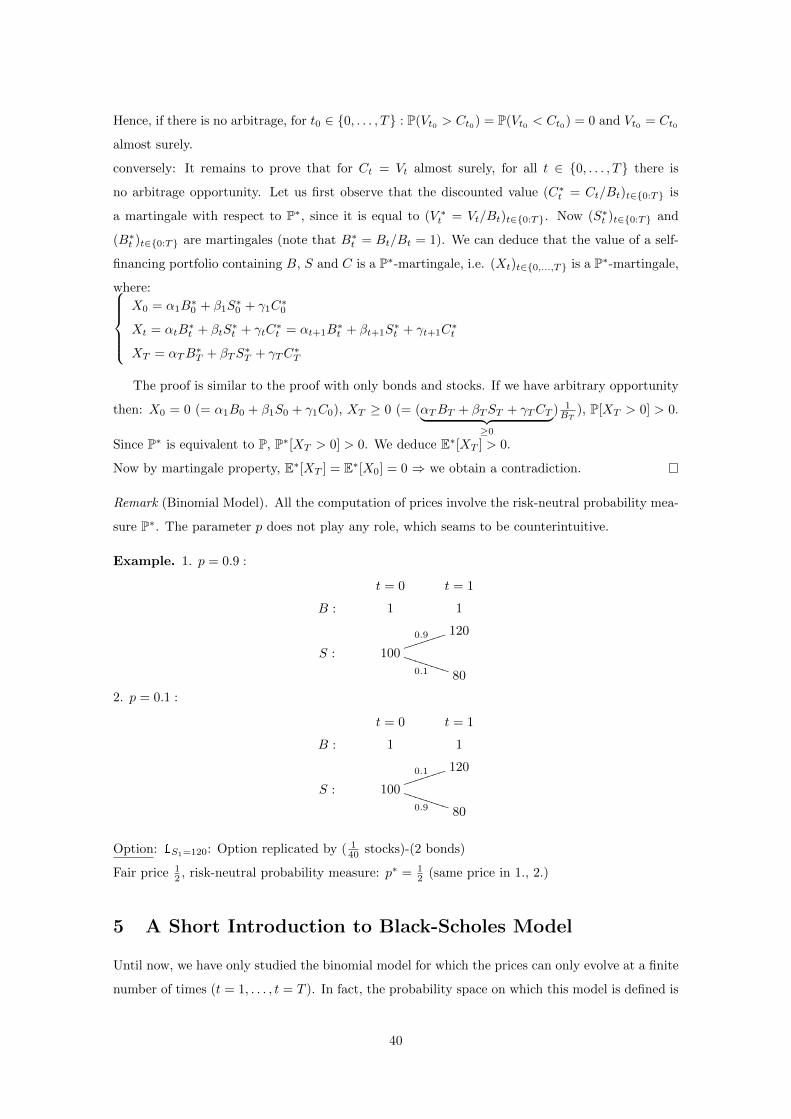
Hence, if there is no arbitrage, for t0 ∈ 0, . . . , T : P(Vt0 > Ct0) = P(Vt0 < Ct0) = 0 and Vt0 = Ct0
almost surely.
conversely: It remains to prove that for Ct = Vt almost surely, for all t ∈ 0, . . . , T there is
no arbitrage opportunity. Let us first observe that the discounted value (C∗t = Ct/Bt)t∈0:T is
a martingale with respect to P∗, since it is equal to (V ∗t = Vt/Bt)t∈0:T. Now (S∗t )t∈0:T and
(B∗t )t∈0:T are martingales (note that B∗t = Bt/Bt = 1). We can deduce that the value of a self-
financing portfolio containing B, S and C is a P∗-martingale, i.e. (Xt)t∈0,...,T is a P∗-martingale,
where:X0 = α1B
∗0 + β1S
∗0 + γ1C
∗0
Xt = αtB∗t + βtS
∗t + γtC
∗t = αt+1B
∗t + βt+1S
∗t + γt+1C
∗t
XT = αTB∗T + βTS
∗T + γTC
∗T
The proof is similar to the proof with only bonds and stocks. If we have arbitrary opportunity
then: X0 = 0 (= α1B0 + β1S0 + γ1C0), XT ≥ 0 (= (αTBT + βTST + γTCT︸ ︷︷ ︸≥0
) 1BT
), P[XT > 0] > 0.
Since P∗ is equivalent to P, P∗[XT > 0] > 0. We deduce E∗[XT ] > 0.
Now by martingale property, E∗[XT ] = E∗[X0] = 0 ⇒ we obtain a contradiction.
Remark (Binomial Model). All the computation of prices involve the risk-neutral probability mea-
sure P∗. The parameter p does not play any role, which seams to be counterintuitive.
Example. 1. p = 0.9 :
t = 0 t = 1
B : 1 1
120
S : 100
0.9 iiiiiii
0.1 UUUUUUUU
80
2. p = 0.1 :
t = 0 t = 1
B : 1 1
120
S : 100
0.1 iiiiiii
0.9 UUUUUUUU
80
Option: 1S1=120: Option replicated by ( 140 stocks)-(2 bonds)
Fair price 12 , risk-neutral probability measure: p∗ = 1
2 (same price in 1., 2.)
5 A Short Introduction to Black-Scholes Model
Until now, we have only studied the binomial model for which the prices can only evolve at a finite
number of times (t = 1, . . . , t = T ). In fact, the probability space on which this model is defined is
40

finite itself, which means that there are only finite number of possible evolution of the prices. This
kind of model has the advantage that the technical problems are reduced to their minimum. For
example, we have no problem of continuity of the trajectories, and we don’t need deal with random
processes in continuous-time. On the other hand, it is intuitively obvious that basic models as the
binomial one are too simple to be realistic. In a real market, the stock prices evolve constantly
and regularly they need to be modeled by a discrete-time model with a huge number of steps and
more than 2 possibilities and each step, or by a continuous model, where trading is possible at
any time. The most basic (but even difficult to state rigorously) continuous-time model is called
Black-Scholes model (introduced in 1973).
In this most simple form, it contains again two assets: a bond and a stock. However their prices
evolve continuously, and intuitively, the model can be viewed as the limit of a binomial when the
frequency of the steps tend to infinity. In this part of the lecture, we show (a little bit) what should
mean this limit. Let us first study the bond price.
The bond price: Let us recall that if the interest rate is r, the bond price at time t ∈ N is
B[i]t = (1 + r)t for the binomial model. Now let us imagine a binomial model where, instead of one
step by unit time, we have N steps by unit of time. In this case, for an interest rate r by unit of
time, we obtain an interest rate (r/N) for each step.
Bond-price: Bt = er·t (r is the interest) (for all t ∈ R+ (infinite horizon-time), or t ∈ [0, T ] (finite
horizon-time)) (no randomness)
Stock-price: Take a limit of binomial model for the number of steps per unit of time →∞. Let us
suppose that one has N steps per unit of time. We take, for each step, a stock price multiplied by
1 + uN with probability pN , and by 1− dN with probability 1− pN .
The parameters uN , dN need to depend on N , otherwise, the fluctuations of the stock price are
stronger and stronger for N →∞. (We need uN , dN “small”) We can write 1+uN = exp (vN ) , 1−
dN = exp (wN ) (vN expected to be positive, wN expected to be negative) (1− dN > 0) with new
parameters vN , wN (pN doesn’t need to depend on N). Let S[N ]t be the stock price at time t. Before
time 1, the number of steps is [tN ]. Hence, S[N ]t = S
[N ]0
Ntexp(1[N ]j ) where 1
[N ]j are independent, P[1
[N ]j = vN ] = pN
P[1[N ]j = wN ] = 1− pN
Take the logarithm. log
(S
[N]t
S[N]0
)=
[Nt]∑j=1
y[N ]j . In which case can we expect a limit model? We
need to have a limit law for the sum[Nt]∑j=1
y[N ]j (because we have a limit N → ∞ for S
[N ]0 ). Let us
take particular parameters satisfying E
[[Nt]∑j=1
y[N ]j
]→ C(t) for some limit C(t) (it is not implied by
convergence in law but it can be “reasonably expected”). The computation of expectation gives:
E
[[Nt]∑j=1
y[N ]j
]=
[Nt]∑j=1
E[y[N ]j
]=
[Nt]∑j=1
E[y[N ]1
]= [Nt] ·E
[y[N ]j
]= [Nt](vNpN +wN (1−pN )). It should
converge to C(t). It is equivalent to Nt(vNpN+wN (1−pN ))⇒ vNpN+wN (1−pN ) should decrease
41
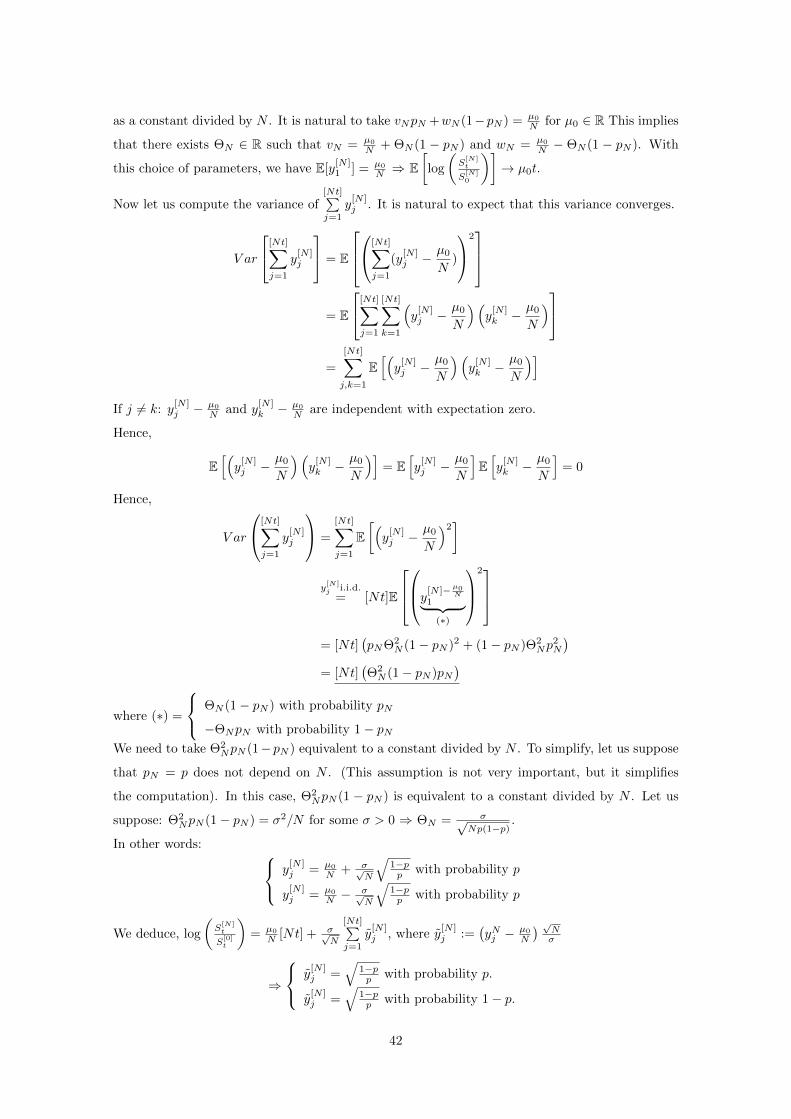
as a constant divided by N . It is natural to take vNpN +wN (1−pN ) = µ0
N for µ0 ∈ R This implies
that there exists ΘN ∈ R such that vN = µ0
N + ΘN (1 − pN ) and wN = µ0
N − ΘN (1 − pN ). With
this choice of parameters, we have E[y[N ]1 ] = µ0
N ⇒ E[log
(S
[N]t
S[N]0
)]→ µ0t.
Now let us compute the variance of[Nt]∑j=1
y[N ]j . It is natural to expect that this variance converges.
V ar
[Nt]∑j=1
y[N ]j
= E
[Nt]∑j=1
(y[N ]j − µ0
N)
2
= E
[Nt]∑j=1
[Nt]∑k=1
(y[N ]j − µ0
N
)(y[N ]k − µ0
N
)=
[Nt]∑j,k=1
E[(y[N ]j − µ0
N
)(y[N ]k − µ0
N
)]If j 6= k: y
[N ]j − µ0
N and y[N ]k − µ0
N are independent with expectation zero.
Hence,
E[(y[N ]j − µ0
N
)(y[N ]k − µ0
N
)]= E
[y[N ]j − µ0
N
]E[y[N ]k − µ0
N
]= 0
Hence,
V ar
[Nt]∑j=1
y[N ]j
=
[Nt]∑j=1
E[(y[N ]j − µ0
N
)2]
y[N]j i.i.d.
= [Nt]E
y[N ]−µ0N
1︸ ︷︷ ︸(∗)
2
= [Nt](pNΘ2
N (1− pN )2 + (1− pN )Θ2Np
2N
)= [Nt]
(Θ2N (1− pN )pN
)where (∗) =
ΘN (1− pN ) with probability pN
−ΘNpN with probability 1− pNWe need to take Θ2
NpN (1− pN ) equivalent to a constant divided by N . To simplify, let us suppose
that pN = p does not depend on N . (This assumption is not very important, but it simplifies
the computation). In this case, Θ2NpN (1 − pN ) is equivalent to a constant divided by N . Let us
suppose: Θ2NpN (1− pN ) = σ2/N for some σ > 0 ⇒ ΘN = σ√
Np(1−p).
In other words: y[N ]j = µ0
N + σ√N
√1−pp with probability p
y[N ]j = µ0
N −σ√N
√1−pp with probability p
We deduce, log
(S
[N]t
S[0]t
)= µ0
N [Nt] + σ√N
[Nt]∑j=1
y[N ]j , where y
[N ]j :=
(yNj −
µ0
N
) √Nσ
⇒
y[N ]j =
√1−pp with probability p.
y[N ]j =
√1−pp with probability 1− p.
42
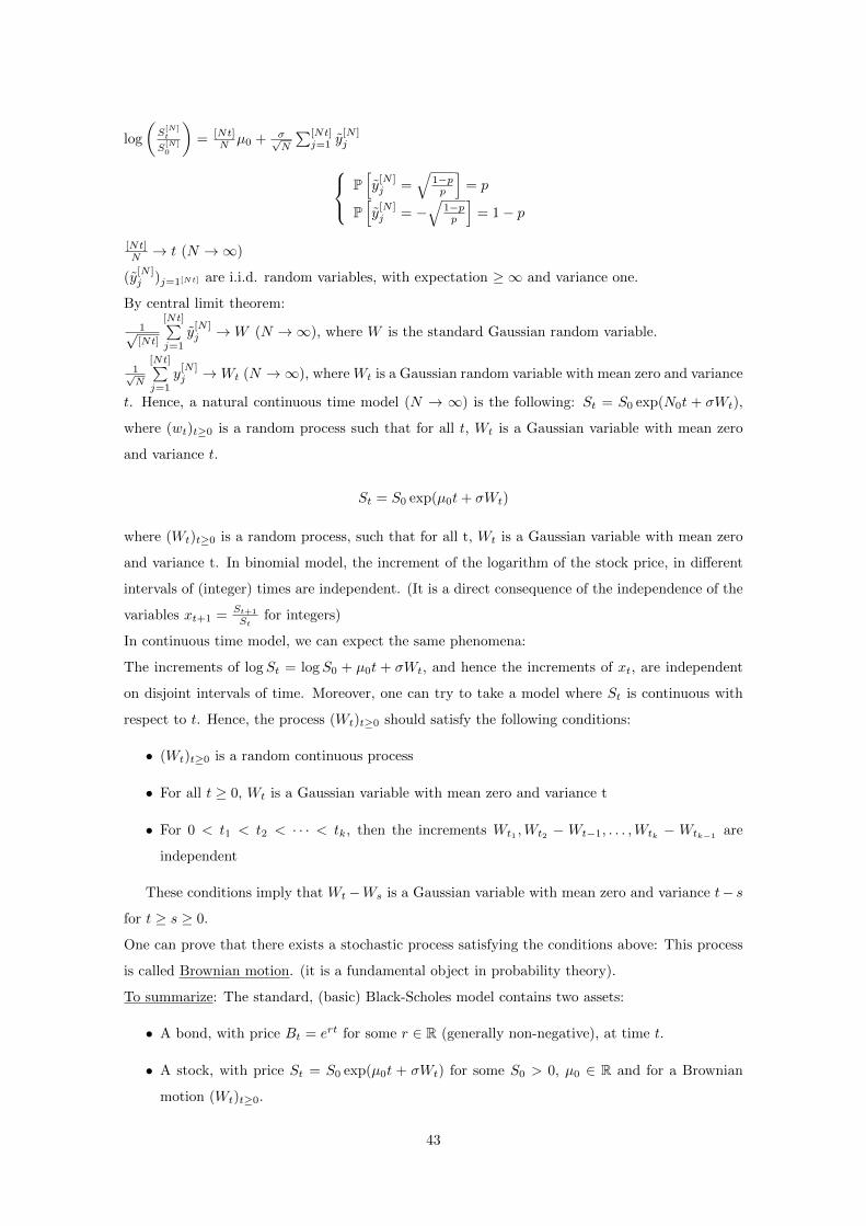
log
(S
[N]t
S[N]0
)= [Nt]
N µ0 + σ√N
∑[Nt]j=1 y
[N ]j P[y[N ]j =
√1−pp
]= p
P[y[N ]j = −
√1−pp
]= 1− p
[Nt]N → t (N →∞)
(y[N ]j )j=1[Nt] are i.i.d. random variables, with expectation ≥ ∞ and variance one.
By central limit theorem:
1√[Nt]
[Nt]∑j=1
y[N ]j →W (N →∞), where W is the standard Gaussian random variable.
1√N
[Nt]∑j=1
y[N ]j →Wt (N →∞), where Wt is a Gaussian random variable with mean zero and variance
t. Hence, a natural continuous time model (N → ∞) is the following: St = S0 exp(N0t + σWt),
where (wt)t≥0 is a random process such that for all t, Wt is a Gaussian variable with mean zero
and variance t.
St = S0 exp(µ0t+ σWt)
where (Wt)t≥0 is a random process, such that for all t, Wt is a Gaussian variable with mean zero
and variance t. In binomial model, the increment of the logarithm of the stock price, in different
intervals of (integer) times are independent. (It is a direct consequence of the independence of the
variables xt+1 = St+1
Stfor integers)
In continuous time model, we can expect the same phenomena:
The increments of logSt = logS0 + µ0t + σWt, and hence the increments of xt, are independent
on disjoint intervals of time. Moreover, one can try to take a model where St is continuous with
respect to t. Hence, the process (Wt)t≥0 should satisfy the following conditions:
• (Wt)t≥0 is a random continuous process
• For all t ≥ 0, Wt is a Gaussian variable with mean zero and variance t
• For 0 < t1 < t2 < · · · < tk, then the increments Wt1 ,Wt2 − Wt−1, . . . ,Wtk − Wtk−1are
independent
These conditions imply that Wt−Ws is a Gaussian variable with mean zero and variance t− s
for t ≥ s ≥ 0.
One can prove that there exists a stochastic process satisfying the conditions above: This process
is called Brownian motion. (it is a fundamental object in probability theory).
To summarize: The standard, (basic) Black-Scholes model contains two assets:
• A bond, with price Bt = ert for some r ∈ R (generally non-negative), at time t.
• A stock, with price St = S0 exp(µ0t + σWt) for some S0 > 0, µ0 ∈ R and for a Brownian
motion (Wt)t≥0.
43

Question. How can model trading?
Portfolio: Modeled by random variables (αt)t≥0 (αt: quantity of bonds at time t), (βt)t≥0 (βt:
quantity of stocks at time t).
αt, βt are measurable with respect to the “information available up to time t”, i.e. the σ-algebra
generated by Ws, s ≤ r.
Values of the portfolio at ti em t: Vt = αtBt + βtSt Vt − Vt−1 = (αtBt + βtSt) − (Vt = αtBt−1 +
βtSt−1) = αt(Bt −Bt−1) + βt(St − St−1).
In continuous time: dVt = αtdBt + βtdSt. Vt − V0 =t∫0
αrdBst∫0
sBs
• Vt − V0 =t∫0
αsdBs +t∫0
βsdSs
• Bs = ers → dBs = r · ersds⇒t∫0
αs · r · ersds (well-defined)
•t∫0
βsdSs has to be well-defined (a stochastic integral) (not obvious at all to construct)
European contingent claim: CT , measurable with respect to the σ-algebra generated by Ws, s ≤ t.
Example. Call option: CT = (ST − k)t.
Essentially (up to non-trivial technical problem) each CT can be replicated in a unique way by
a self-financing portfolio. (totally informal)
The Black-Scholes model is complete and viable. (There is a notion of arbitrage). This gives a
“fair price to the options”: St = S0 exp(µ0t+ σWt)
Discounted stock price: S∗t = StBt
= S0 exp((µ0 − r)t+ σWt).
This is not a martingale in general. But one can change the probability, which gives the risk-neutral
probability measure (called “Girsanov transformation”). Under this new measure (Wt)t≥0 is not
a Brownian motion anymore, but S∗t = S0 exp((µ0 − r)t + σWt) = S0 exp(−σ2
2 t + σBt), where
(Bt)t≥0 is a Brownian motion under the risk-neutral probability measure.
Hence, S∗t is a martingale (consequence of the properties of the Brownian motion). V ∗t = VtBt
is
also a martingale for all “reasonable” self-financing portfolio. ⇒ Fair price of CT (as for binomial
model: E∗[CT ]/Bt)
Call option: E∗[(ST − k)t|Bt]︸ ︷︷ ︸Can be explicitely computed and we obtain Black-Scholes formula.
44