1

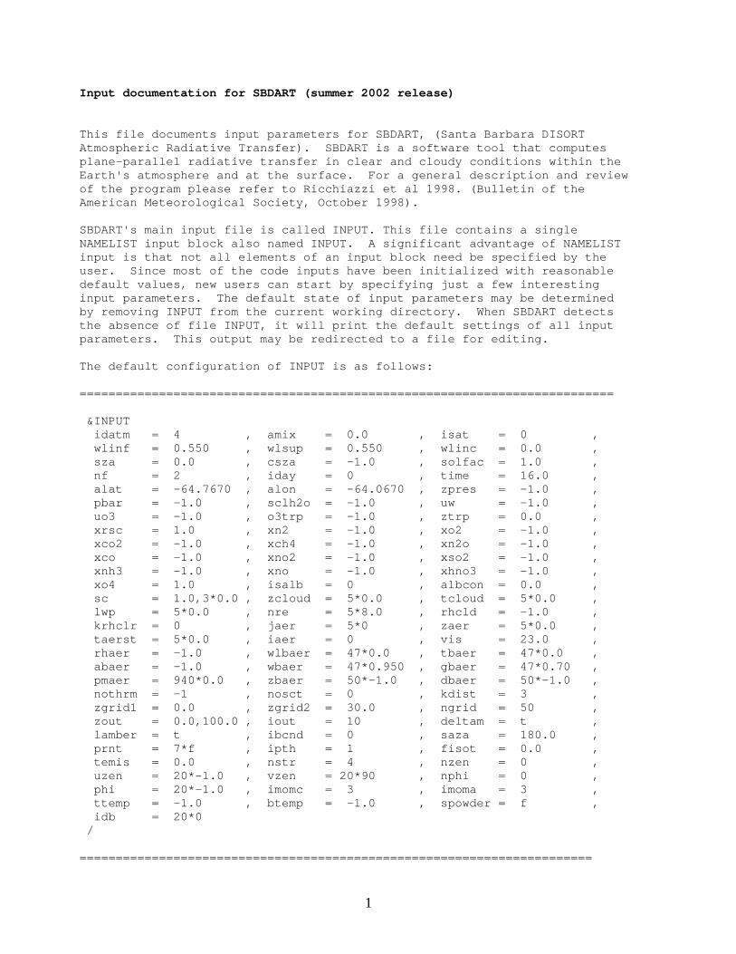
Input documentation for SBDART (summer 2002 release) This file documents input parameters for SBDART, (Santa Barbara DISORT Atmospheric Radiative Transfer). SBDART is a software tool that computes plane-parallel radiative transfer in clear and cloudy conditions within the Earth's atmosphere and at the surface. For a general description and review of the program please refer to Ricchiazzi et al 1998. (Bulletin of the American Meteorological Society, October 1998). SBDART's main input file is called INPUT. This file contains a single NAMELIST input block also named INPUT. A significant advantage of NAMELIST input is that not all elements of an input block need be specified by the user. Since most of the code inputs have been initialized with reasonable default values, new users can start by specifying just a few interesting input parameters. The default state of input parameters may be determined by removing INPUT from the current working directory. When SBDART detects the absence of file INPUT, it will print the default settings of all input parameters. This output may be redirected to a file for editing. The default configuration of INPUT is as follows: ========================================================================== &INPUT idatm = 4 , amix = 0.0 , isat = 0 , wlinf = 0.550 , wlsup = 0.550 , wlinc = 0.0 , sza = 0.0 , csza = -1.0 , solfac = 1.0 , nf = 2 , iday = 0 , time = 16.0 , alat = -64.7670 , alon = -64.0670 , zpres = -1.0 , pbar = -1.0 , sclh2o = -1.0 , uw = -1.0 , uo3 = -1.0 , o3trp = -1.0 , ztrp = 0.0 , xrsc = 1.0 , xn2 = -1.0 , xo2 = -1.0 , xco2 = -1.0 , xch4 = -1.0 , xn2o = -1.0 , xco = -1.0 , xno2 = -1.0 , xso2 = -1.0 , xnh3 = -1.0 , xno = -1.0 , xhno3 = -1.0 , xo4 = 1.0 , isalb = 0 , albcon = 0.0 , sc = 1.0,3*0.0 , zcloud = 5*0.0 , tcloud = 5*0.0 , lwp = 5*0.0 , nre = 5*8.0 , rhcld = -1.0 , krhclr = 0 , jaer = 5*0 , zaer = 5*0.0 , taerst = 5*0.0 , iaer = 0 , vis = 23.0 , rhaer = -1.0 , wlbaer = 47*0.0 , tbaer = 47*0.0 , abaer = -1.0 , wbaer = 47*0.950 , gbaer = 47*0.70 , pmaer = 940*0.0 , zbaer = 50*-1.0 , dbaer = 50*-1.0 , nothrm = -1 , nosct = 0 , kdist = 3 , zgrid1 = 0.0 , zgrid2 = 30.0 , ngrid = 50 , zout = 0.0,100.0 , iout = 10 , deltam = t , lamber = t , ibcnd = 0 , saza = 180.0 , prnt = 7*f , ipth = 1 , fisot = 0.0 , temis = 0.0 , nstr = 4 , nzen = 0 , uzen = 20*-1.0 , vzen = 20*90 , nphi = 0 , phi = 20*-1.0 , imomc = 3 , imoma = 3 , ttemp = -1.0 , btemp = -1.0 , spowder = f , idb = 20*0 / =======================================================================

2

NOTE: Unfortunately, many fortran compilers produce rather cryptic error messages in response to improper NAMELIST input files. Here are three common NAMELIST error messages and their meaning: 1. ERROR MESSAGE: invalid reference to variable in NAMELIST input MEANING: you misspelled one of the NAMELIST variable names 2. ERROR MESSAGE: too many values for NAMELIST variable MEANING: you specified too many values for a variable, most likely because you separated variables by more than one comma. 2. ERROR MESSAGE: end-of-file during read or namelist block INPUT not found MEANING: There are two possibilities: A) you didn't include a NAMELIST block specifier (INPUT, DINPUT or END) or you misspelled it; or B) You used the wrong character to signify a namelist block name. FORTRAN90 expects the namelist blocks to start with &<name> and end with /, but most FORTRAN77 compilers used the $<name>, $END convention. Other input files are sometimes required by SBDART: atms.dat -- atmospheric profile (see input quantity IDATM) aerosol.dat -- aerosol information (see input quantity IAER) albedo.dat -- spectral surface albedo (see input quantity ISALB) filter.dat -- sensor filter function (see input quantity ISAT) solar.dat -- solar spectrum (see input quantity NF) usrcld.dat -- cloud vertical profile (see input quantity TCLOUD) SBDART usually lists computational results directly to the standard output device (i.e., the terminal, if run interactively). However, some warning messages are written to files named SBDART_WARNING.?? where the question marks indicate a warning message number. When running SBDART iteratively over many inputs, the SBDART_WARNING files will only be created once, on the first iteration that generated the warning condition. The warning files contain a warning message and a copy of the input file that triggered the warning.

3

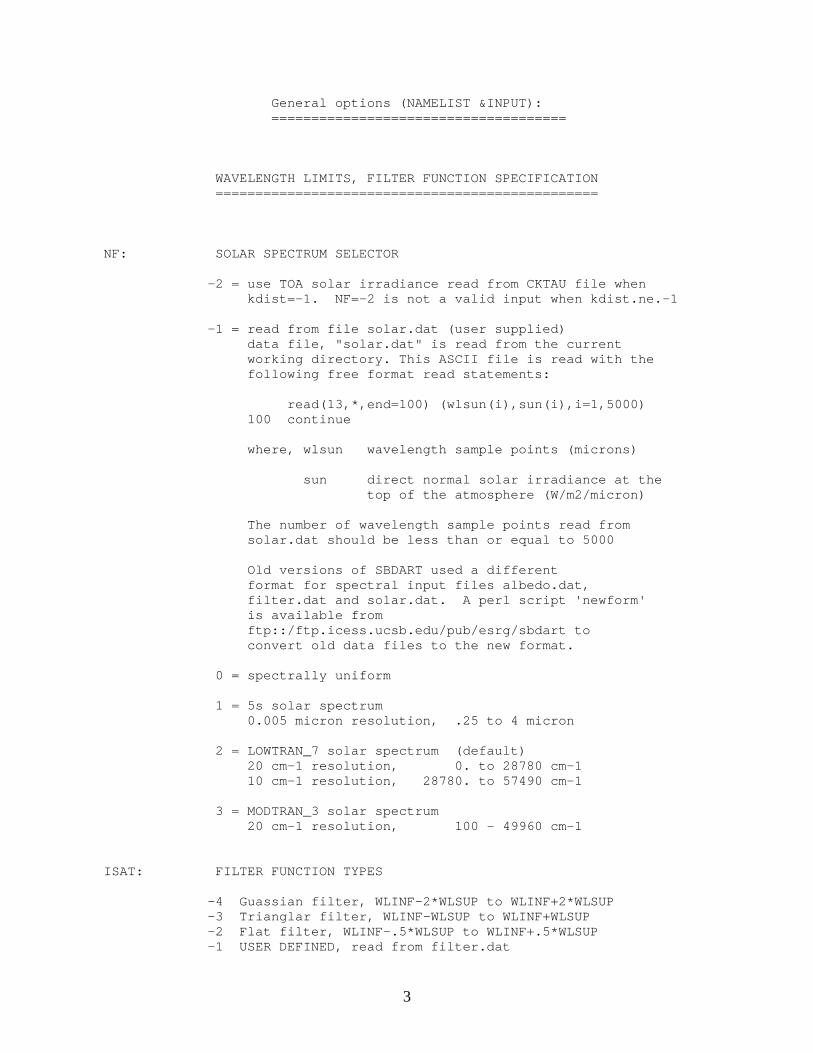
General options (NAMELIST &INPUT): ===================================== WAVELENGTH LIMITS, FILTER FUNCTION SPECIFICATION ================================================ NF: SOLAR SPECTRUM SELECTOR -2 = use TOA solar irradiance read from CKTAU file when kdist=-1. NF=-2 is not a valid input when kdist.ne.-1 -1 = read from file solar.dat (user supplied) data file, "solar.dat" is read from the current working directory. This ASCII file is read with the following free format read statements: read(13,*,end=100) (wlsun(i),sun(i),i=1,5000) 100 continue where, wlsun wavelength sample points (microns) sun direct normal solar irradiance at the top of the atmosphere (W/m2/micron) The number of wavelength sample points read from solar.dat should be less than or equal to 5000 Old versions of SBDART used a different format for spectral input files albedo.dat, filter.dat and solar.dat. A perl script 'newform' is available from ftp::/ftp.icess.ucsb.edu/pub/esrg/sbdart to convert old data files to the new format. 0 = spectrally uniform 1 = 5s solar spectrum 0.005 micron resolution, .25 to 4 micron 2 = LOWTRAN_7 solar spectrum (default) 20 cm-1 resolution, 0. to 28780 cm-1 10 cm-1 resolution, 28780. to 57490 cm-1 3 = MODTRAN_3 solar spectrum 20 cm-1 resolution, 100 - 49960 cm-1 ISAT: FILTER FUNCTION TYPES -4 Guassian filter, WLINF-2*WLSUP to WLINF+2*WLSUP -3 Trianglar filter, WLINF-WLSUP to WLINF+WLSUP -2 Flat filter, WLINF-.5*WLSUP to WLINF+.5*WLSUP -1 USER DEFINED, read from filter.dat

4

0 WLINF TO WLSUP WITH FILTER FUNCTION = 1 (default) NOTE: if ISAT=0 and KDIST=-1, then the values of WLINF and WLSUP only have an effect if they have been changed from their default values such that WLINF .ne. WLSUP. Otherwise the wavelength sample points are as specified in the CKTAU file. 1 METEO 2 GOES(EAST) 3 GOES(WEST) 4 AVHRR1(NOAA8) 5 AVHRR2(NOAA8) 6 AVHRR1(NOAA9) 7 AVHRR2(NOAA9) 8 AVHRR1(NOAA10) 9 AVHRR2(NOAA10) 10 AVHRR1(NOAA11) 11 AVHRR2(NOAA11) 12 GTR-100 ch1 13 GTR-100 ch2 14 GTR-100 410nm channel 15 GTR-100 936nm channel 16 MFRSR 415nm channel 17 MFRSR 500nm channel 18 MFRSR 610nm channel 19 MFRSR 665nm channel 20 MFRSR 862nm channel 21 MFRSR 940nm channel 22 AVHRR3 (nominal) 23 AVHRR4 (nominal) 24 AVHRR5 (nominal) 25 Biological action spectra for DNA damage by UVB radiation 26 AIRS1 380-460nm 27 AIRS2 520-700nm 28 AIRS3 670-975nm 29 AIRS4 415-1110nm NOTE: If ISAT=-1 a user supplied filter data file "filter.dat" is read from the current working directory. This ASCII file is read with the following free format read (numbers may be separated by spaces, commas or carriage returns); read(13,*,end=100) (wlfilt(i),filt(i),i=1,huge(0)) 100 continue where, wlfilt wavelength sample points (microns) filt filter response value (unitless) The number of wavelength sample points read from filter.dat should be less than or equal to 1000

5

This file format is new. Previous versions of SBDART used a different format for spectral input files albedo.dat, filter.dat and solar.dat. A perl script 'newform' is available from ftp::/ftp.icess.ucsb.edu/pub/esrg/sbdart to convert old data files to the new format. WLINF: lower wavelength limit when ISAT=0 (WLINF > .250 microns) central wavelength when ISAT=-2,-3,-4 WLSUP: upper wavelength limit when ISAT=0 (WLSUP < 100.0 microns) equivalent width when ISAT=-2,-3,-4 NOTE: If ISAT eq -2, a rectangular filter (constant with wavelength) is used, with central wavelength at WLINF and an equivalent width of WLSUP (full width = WLSUP) If ISAT eq -3, a triangular filter function is used with the central wavelength at WLINF and an equivalent width of WLSUP (full width = 2*WLSUP) (filter function is zero at end points, and one at WLINF). If ISAT eq -4, a gaussian filter function is used with the central wavelength at WLINF and an equivalent width of WLSUP (full width = 4*WLSUP) If output is desired at a single wavelength, set WLINF=WLSUP and ISAT=0. In this case, SBDART will set WLINC=1 (the user specified value of WLINC is ignored) and the output will be in units of (W/m2/um) for irradiance and (W/m2/um/sr) for radiance. WLINC: This parameter specifies the spectral resolution of the SBDART run. Though the spectral limits of the calculation are always input in terms of wavelength, the spectral step size can be specified in terms of constant increments of wavelength, log(wavelength) [same as constant increment of log(wavenumber)] or wavenumber. Which one to choose depends on where in the spectral bandpass you want to place the most resolution. Since SBDART is based on LOWTRAN7 band models, which have a spectral resolution of 20 cm-1, it would be extreme overkill to allow spectral step size less than 1 cm-1. On the other hand a spectral resolution coarser than 1 um is also pretty useless. Therefore the way WLINC is interpreted depends on whether it is less than zero, between zero and one, or greater than 1. * WLINC = 0 (the default) => wavelength increment is equal to 0.005 um or 1/10 the wavelength range, which

6

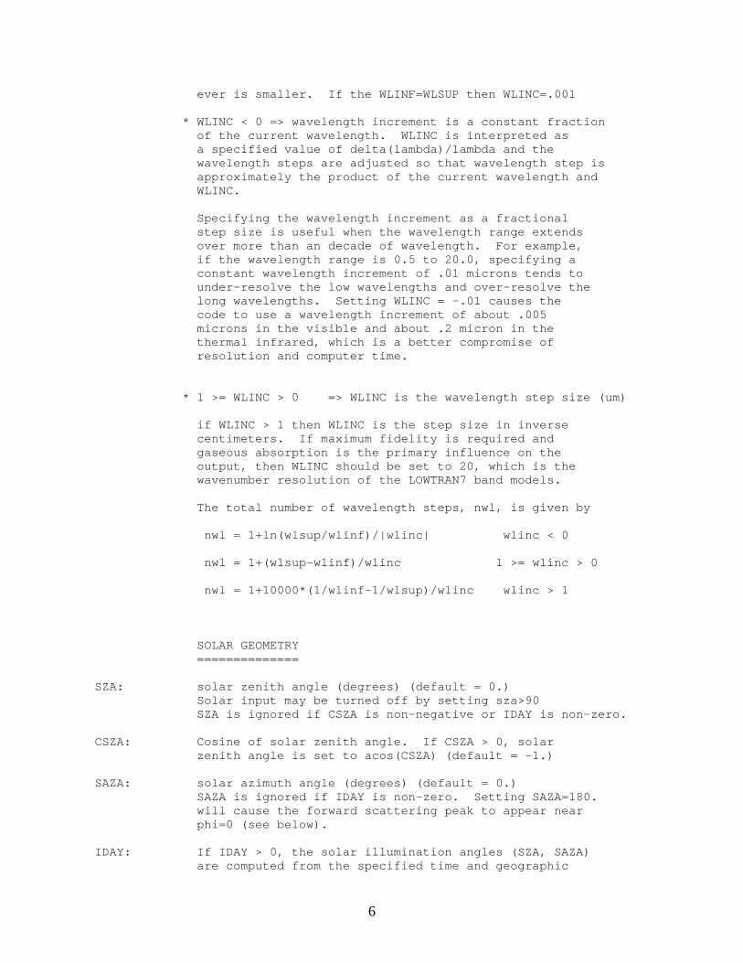
ever is smaller. If the WLINF=WLSUP then WLINC=.001 * WLINC < 0 => wavelength increment is a constant fraction of the current wavelength. WLINC is interpreted as a specified value of delta(lambda)/lambda and the wavelength steps are adjusted so that wavelength step is approximately the product of the current wavelength and WLINC. Specifying the wavelength increment as a fractional step size is useful when the wavelength range extends over more than an decade of wavelength. For example, if the wavelength range is 0.5 to 20.0, specifying a constant wavelength increment of .01 microns tends to under-resolve the low wavelengths and over-resolve the long wavelengths. Setting WLINC = -.01 causes the code to use a wavelength increment of about .005 microns in the visible and about .2 micron in the thermal infrared, which is a better compromise of resolution and computer time. * 1 >= WLINC > 0 => WLINC is the wavelength step size (um) if WLINC > 1 then WLINC is the step size in inverse centimeters. If maximum fidelity is required and gaseous absorption is the primary influence on the output, then WLINC should be set to 20, which is the wavenumber resolution of the LOWTRAN7 band models. The total number of wavelength steps, nwl, is given by nwl = 1+ln(wlsup/wlinf)/|wlinc| wlinc < 0 nwl = 1+(wlsup-wlinf)/wlinc 1 >= wlinc > 0 nwl = 1+10000*(1/wlinf-1/wlsup)/wlinc wlinc > 1 SOLAR GEOMETRY ============== SZA: solar zenith angle (degrees) (default = 0.) Solar input may be turned off by setting sza>90 SZA is ignored if CSZA is non-negative or IDAY is non-zero. CSZA: Cosine of solar zenith angle. If CSZA > 0, solar zenith angle is set to acos(CSZA) (default = -1.) SAZA: solar azimuth angle (degrees) (default = 0.) SAZA is ignored if IDAY is non-zero. Setting SAZA=180. will cause the forward scattering peak to appear near phi=0 (see below). IDAY: If IDAY > 0, the solar illumination angles (SZA, SAZA) are computed from the specified time and geographic

7

coordinates using an internal solar ephemeris algorithm (see subroutine zensun). IDAY is the number of days into a standard "year", with IDAY=1 and the 1st of January and IDAY=365 on the 31st of December if IDAY > 365, IDAY is replaced internally by mod(IDAY-1,365)+1. If IDAY < 0, the code writes the values of abs(iday),time, alat,alon,sza,azm, and solfac to standard output and exits. TIME: UTC time (Grenwich) in decimal hours ALAT: latitude of point on earth's surface ALON: east longitude of point on earth's surface NOTE: TIME, ALAT and ALON are ignored if IDAY .eq. 0 SOLFAC: solar distance factor. Use this factor to account for seasonal variations of the earth-sun distance. If R is the earth-sun distance in Astronomical Units then SOLFAC=1./R**2. SOLFAC is set internally when the solar geometry is set through IDAY, TIME, ALAT and ALON. In this case SOLFAC is set to, -2 SOLFAC = ( 1.-eps*cos(2*pi*(IDAY-perh)/365) ) where eps = orbital eccentricity = 0.01673 and perh = day of perihelion = 2 (jan 2) NOTE: seasonal variations in earth-sun distance produce a +/-3.4% perturbation in the TOA solar flux. This factor should be included when making detailed comparisons to surface measurements. NOSCT: aerosol scattering mode used for boundary layer aerosols: 0 normal scattering and absorption treatment 1 reduce optical depth by (1-ssa*asym), set ssa=0 2 set ssa=0 3 reduce optical depth by (1-ssa), set ssa=0 where ssa=single scattering albedo, and asym=asymmetry factor nosct does not affect the stratospheric aerosol models or the iaer=5 boundary layer model. SURFACE REFLECTANCE PROPERTIES ============================== ISALB: SURFACE ALBEDO FEATURE -1 -spectral surface albedo read from "albedo.dat" 0 -user specified, spectrally uniform albedo set with ALBCON 1 -snow 2 -clear water 3 -lake water

8

4 -sea water 5 -sand (data range 0.4 - 2.3um) 6 -vegetation (data range 0.4 - 2.6um) 7 -ocean water brdf, includes bio-pigments, foam, and sunglint additional input parameters provided in SC. 8 -Hapke analytic brdf model. additional input parameters provided in SC. 9 -Ross-thick Li-sparse brdf model. additional input parameters in SC. NOTE: isalb = 7, 8, 9 causes sbdart to use a non-Lambertian surface reflectance. Since the reflectance BRDF must first be expanded in terms of orthogonal functions, this mode of operation is somewhat more time consuming than the normal Lambertian reflectance models, In some cases flux calculations may be accurately computed in Lambertian mode by using directional albedo computed from the brdf, assuming all the incomming radiation is along the solar beam direction. Of course this approach will probably fail in cases where the solar direct beam doesn't dominate the downwelling radiation (e.g., in the infrared or under clouds). SBDART may be run with directional albedos by setting isalb to -7, -8 or -9. 10 -combination of snow, seawater, sand and vegetation partition factors set by input quantity SC NOTE: If ISALB=-1 a user supplied spectral reflectance file "albedo.dat" is read from the current working directory. This ASCII file is read with the following free format read (numbers may be separated by spaces, commas or carriage returns); read(13,*,end=100) (wlalb(i),alb(i),i=1,huge(0)) 100 continue where, wlalb wavelength sample points (microns) alb spectral albedo (unitless) The number of wavelength sample points read from albedo.dat should be less than or equal to 1000 The user specified reflectance may cover any wavelength range and have arbitrarily high resolution. This contrasts with the standard reflectance models (sand, vegetation, lake water and sea water) which are only specified in in the range .25 to 4 um at 5nm resolution. Prior to version 2.0, SBDART used a different format

9

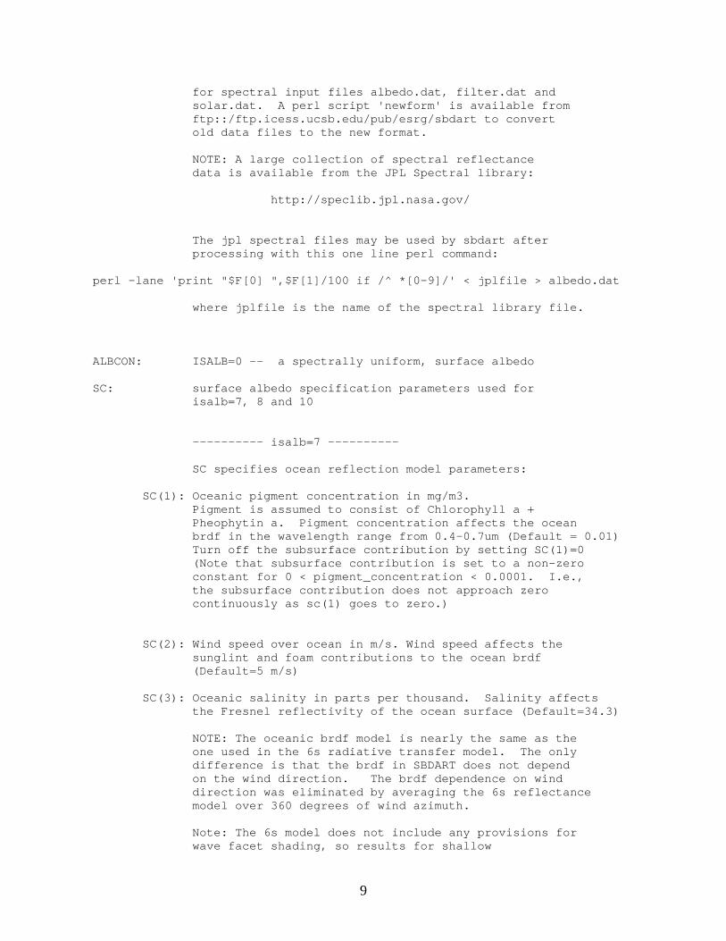
for spectral input files albedo.dat, filter.dat and solar.dat. A perl script 'newform' is available from ftp::/ftp.icess.ucsb.edu/pub/esrg/sbdart to convert old data files to the new format. NOTE: A large collection of spectral reflectance data is available from the JPL Spectral library: http://speclib.jpl.nasa.gov/ The jpl spectral files may be used by sbdart after processing with this one line perl command: perl -lane 'print "$F[0] ",$F[1]/100 if /^ *[0-9]/' < jplfile > albedo.dat where jplfile is the name of the spectral library file. ALBCON: ISALB=0 -- a spectrally uniform, surface albedo SC: surface albedo specification parameters used for isalb=7, 8 and 10 ---------- isalb=7 ---------- SC specifies ocean reflection model parameters: SC(1): Oceanic pigment concentration in mg/m3. Pigment is assumed to consist of Chlorophyll a + Pheophytin a. Pigment concentration affects the ocean brdf in the wavelength range from 0.4-0.7um (Default = 0.01) Turn off the subsurface contribution by setting SC(1)=0 (Note that subsurface contribution is set to a non-zero constant for 0 < pigment_concentration < 0.0001. I.e., the subsurface contribution does not approach zero continuously as sc(1) goes to zero.) SC(2): Wind speed over ocean in m/s. Wind speed affects the sunglint and foam contributions to the ocean brdf (Default=5 m/s) SC(3): Oceanic salinity in parts per thousand. Salinity affects the Fresnel reflectivity of the ocean surface (Default=34.3) NOTE: The oceanic brdf model is nearly the same as the one used in the 6s radiative transfer model. The only difference is that the brdf in SBDART does not depend on the wind direction. The brdf dependence on wind direction was eliminated by averaging the 6s reflectance model over 360 degrees of wind azimuth. Note: The 6s model does not include any provisions for wave facet shading, so results for shallow

10

illumination or viewing directions may be incorrect. Additional information is available from "Second Simulation of the Satellite Signal in the Solar Spectrum (6S), user's guide" by Vermote, E., D. Tanre, J.L. Deuze, M. Herman, and J.J. Morcrette (1995). ---------- isalb=8 ---------- SC specifies Hapke analytic brdf model parameters: SC(1): Single scattering albedo of surface particles SC(2): Asymmetry factor of scattering by surface particles SC(3): Magnitude of hot spot (opposition effect) SC(4): Width of hot spot NOTE: This model is based on Hapke, 1981 also see P. Pinet, A. Cord, S. Chevrel and Y. Daydou, (2003): 'Experimental determination of the Hapke parameters for planetary regolith surface analogs' Generic vegetation (actually clover), may be described with sc=0.101,-0.263, 0.589, 0.046. (From Pinty and Verstraete, 1991). Snow may be described with sc=0.99, 0.6, 0.0, 0.995. (From Domingue et al., 1997; and Verbiscer and Veverka, 1990). ---------- isalb=9 ---------- SC specifies the Ross-thick Li-sparse brdf model parameters SC(1)=isotropic coefficient SC(2)=volumetric coefficient SC(3)=geometric shadowing coefficient SC(4)=hot spot magnitude SC(5)=hot spot width (Ross, 1981; Li and Strahler, 1992). ---------- isalb=10 ---------- SC specifies mixing ratios snow, ocean, sand and vegetation Composite albedo fractions (applies only when ISALB=10) SC(1): fraction of snow SC(2): fraction of ocean SC(3): fraction of sand SC(4): fraction of vegetation NOTE: SC(1)+SC(2)+SC(3)+SC(4) need not sum to 1. Thus, it is possible to use the SC factor to boost the overall reflectance of a given surface type. For example, SC=0,0,2,0 yields

11

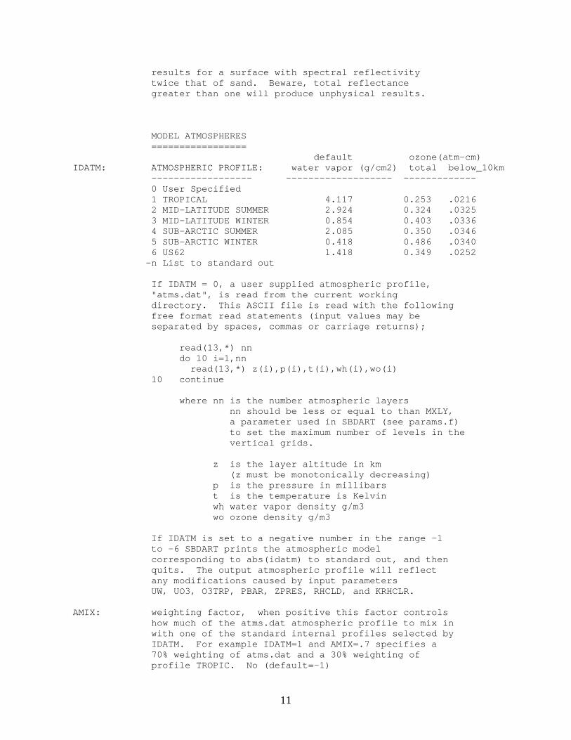
results for a surface with spectral reflectivity twice that of sand. Beware, total reflectance greater than one will produce unphysical results. MODEL ATMOSPHERES ================= default ozone(atm-cm) IDATM: ATMOSPHERIC PROFILE: water vapor (g/cm2) total below_10km ------------------ ------------------- ------------- 0 User Specified 1 TROPICAL 4.117 0.253 .0216 2 MID-LATITUDE SUMMER 2.924 0.324 .0325 3 MID-LATITUDE WINTER 0.854 0.403 .0336 4 SUB-ARCTIC SUMMER 2.085 0.350 .0346 5 SUB-ARCTIC WINTER 0.418 0.486 .0340 6 US62 1.418 0.349 .0252 -n List to standard out If IDATM = 0, a user supplied atmospheric profile, "atms.dat", is read from the current working directory. This ASCII file is read with the following free format read statements (input values may be separated by spaces, commas or carriage returns); read(13,*) nn do 10 i=1,nn read(13,*) z(i),p(i),t(i),wh(i),wo(i) 10 continue where nn is the number atmospheric layers nn should be less or equal to than MXLY, a parameter used in SBDART (see params.f) to set the maximum number of levels in the vertical grids. z is the layer altitude in km (z must be monotonically decreasing) p is the pressure in millibars t is the temperature is Kelvin wh water vapor density g/m3 wo ozone density g/m3 If IDATM is set to a negative number in the range -1 to -6 SBDART prints the atmospheric model corresponding to abs(idatm) to standard out, and then quits. The output atmospheric profile will reflect any modifications caused by input parameters UW, UO3, O3TRP, PBAR, ZPRES, RHCLD, and KRHCLR. AMIX: weighting factor, when positive this factor controls how much of the atms.dat atmospheric profile to mix in with one of the standard internal profiles selected by IDATM. For example IDATM=1 and AMIX=.7 specifies a 70% weighting of atms.dat and a 30% weighting of profile TROPIC. No (default=-1)

12

UW: integrated water vapor amount (G/CM2) UO3: integrated ozone concentration (ATM-CM) above the level ZTRP. The default value of ZTRP=0, so UO3 usally specifies the total ozone column. If UO3 is negative the original ozone density is used. (default=-1) NOTE: 1 atm-cm = 1000 Dobson Units NOTE: Use UW or UO3 to set the integrated amounts of water vapor or ozone in the model atmosphere. Aside from multiplicative factors the vertical profile will be that of the original model atmosphere set by IDATM. The original unmodified density profile is used when UW or UO3 is negative. O3TRP: integrated ozone concentration (ATM-CM) in troposphere. i.e., for z.lt.ZTRP. The original tropospheric density (set with IDATM) is used when O3TRP is negative. (default=-1.) ZTRP: The altitude of the tropopause. The parameters UO3 and O3TRP sets the total column ozone in the stratosphere and troposphere, respectively. Note: since the default value of ZTRP is zero, UO3 normally sets the integrated ozone amount of the entire atmosphere (default=0). XN2: volume mixing ratio of N2 (PPM, default = 781000.00 ) XO2: volume mixing ratio of O2 (PPM, default = 209000.00 ) XCO2: volume mixing ratio of CO2 (PPM, default = 360.00 ) XCH4: volume mixing ratio of CH4 (PPM, default = 1.74 ) XN2O: volume mixing ratio of N2O (PPM, default = 0.32 ) XCO: volume mixing ratio of CO (PPM, default = 0.15 ) XNH3: volume mixing ratio of NH3 (PPM, default = 5.0e-4) XSO2: volume mixing ratio of SO2 (PPM, default = 3.0e-4) XNO: volume mixing ratio of NO (PPM, default = 3.0e-4) XHNO3: volume mixing ratio of HNO3 (PPM, default = 5.0e-5) XNO2: volume mixing ratio of NO2 (PPM, default = 2.3e-5) NOTE: Setting any of these factors to -1 causes that atmospheric component to retain its nominal mixing ratio defined in the US62 atmosphere (as listed above). The volume mixing ratio (VMR) of a given species is adjusted by specifying the surface value of its VMR in PPM. The entire altitude profile is multiplied by the ratio of the user specified VMR and the nominal surface VMR. There are no further re-normalizations of the VMR. Thus, the total of all the VMRs may be greater or less than 10^6. By the way, the

13

default set of VMRs do not add up to 10^6 because of the exclusion of the noble gases which do not have any radiative effects. XRSC: sensitivity factor for Rayleigh scattering (default=1) This factor varies the strength of Rayleigh scattering for sensitivity studies. XO4 sensitivity factor to adjust strength of absorption by oxygen collisional complexes (default=1, see comments in subroutine o4cont) PBAR: surface pressure in millibars. PBAR > 0 causes each pressure to be multiplied by the factor (PBAR/P0) where P0 is the surface pressure of the original atmosphere. The absorption due to mixed gases is affected, but absorption by ozone and water vapor is not (they are separately controlled by UW and UO3). The Rayleigh scattering optical depth is proportional to the PBAR/P0 factor. PBAR = 0 disables Rayleigh scattering and all atmospheric absorption (including water vapor and ozone). Scattering by aerosols or clouds is not affected. PBAR < 0, causes the original pressure profile to be used. (this is the default) NOTE: PBAR has no effect of the CKTAU optical depths. ZPRES: Surface altitude in kilometers. This parameter is just an alternate way of setting the surface pressure, and should not be set when PBAR is specified. When ZPRES is set PBAR is obtained by logarithmic interpolation on the current model's atmosphere pressure and altitude arrays. Changing ZPRES does not alter other parameters in the atmospheric model in any way. Note that setting a large value of ZPRES may push the tropopause (where dT/dz=0) to an unrealistically high altitude. SCLH2O: Water vapor scale height in km. If SCLH2O .gt. 0, then water vapor is vertically distributed as exp(-z/SCLH2O) If SCLH2O .le. 0, then the original vertical profile is used. Changing SCLH2O has no effect on the total water vapor amount.

14

CLOUD PARAMETERS ================ ZCLOUD: Altitude of cloud layers (km) (up to 5 values), Cloud layers may be specified in two ways. To specify separate cloud layers, set ZCLOUD to a sequence of monotonically increasing altitudes. A cloud layer with optical depth TCLOUD(j) will start at the highest computation level for which z(i).le.ZCLOUD(j)+.001 and will extend to the next higher level, z(i+1). To specify a range of altitudes which will be filled by cloud, tag the second element of the range with a minus sign. In this case the element of TCLOUD that corresponds to the negative element of ZCLOUD specifies the gradient of the optical depth. Setting this element of TCLOUD to 1 causes a uniform opacity between the lower and upper limits of the cloud layer. See description of TCLOUD input. Consider, zcloud=1,-3,10,-15 tcloud=4, 1, 8, 1 nre =6, 6, 10, 20 In this example two continuous cloud layers are defined, the lower one extends from 1 to 3 km and has a total optical depth of 4 and an effective radius of 6um. The upper cloud layer extends from 10 to 15 km, has a total optical thickness of 8 and a sliding value of effective radius which starts 10um at the bottom of the cloud and ramps up to 20um at 15km The ramping function is logarithmic, i.e., nre(12km)=10*(20/10)**((12-10)/15-10)). Note that the actual location of the cloud layers is determined by the resolution and placement of vertical grid points in SBDART, as explained below. SBDART puts the i'th cloud layer at the highest vertical grid point, k, such that z(k) .le. abs(ZCLOUD(i)+.001) NOTE: A cloud with a nominal altitude equal to that of one of the computational layer altitudes, Z(K), actually extends from Z(k) to the next higher grid point. For example, a cloud layer at Z(k) will not affect the direct beam flux at Z(k+1) (one layer above) but will strongly affect it at Z(k). (You can check this out your self by setting IOUT=10 and ZCLOUD=1 and messing around with ZOUT to get outputs just above or below the cloud). Suppose the bottom of your computational grid looks like k z(k) ... ... 6 2.5

15

5 2.0 4 1.5 3 1.0 2 0.5 1 0.0 Consider this input, ZCLOUD=1.0, -6.0, 4.0, -9.0 TCLOUD=50., 1.0, 10., 1.0 NRE = 8., 8, 20., 20. Here two overlapping cloud decks are specified, one extending from 1 to 6 km with a total optical thickness of 50, and the other from 4 to 9 km with a total thickness of 10. Since the total cloud optical thickness is spread over the total altitude range we would have 10 optical depths per km for the lower cloud deck and 2 optical depths per km for the second. The code adds the effects of both cloud decks in the region of overlap. Scattering parameters (e.g., single scattering albedo) in the overlap region are given by the weighted averages of the values computed from the mie scattering database using effective radius appropriate to each cloud deck, and weighting according to the opacity contributed by each cloud deck. cloud opacity scattering optical (km-1) parameters depth 6-9 km 6 2 mie(20) 4-6 km 24 12 [mie(10)*10+mie(20)*2]/12 1-4 km 30 10 mie(10) total 60 If you have any doubt about where the code is putting the cloud, set IDB(5)=1 (see below) to get a diagnostic print out of cloud optical depth. NOTE: do not try to put an ice cloud (NRE < 0) in a cloud layer range which includes water cloud (2 le NRE le 128). In other words this specification won't work: ZCLOUD = 1,-4 TCLOUD = 1, 1 NRE = 8,-1 TCLOUD: Optical thickness of cloud layer, (up to 5 values) TCLOUD specifies the cloud optical depth at a wavelength of 0.55um. The cloud optical depth at other wavelengths is computed using the relation, tau = TCLOUD*Q(wl)/Q(0.55um),

16

where Q is the extinction efficiency, which is a function of effective radius and wavelength (see discussion of LWP for a definition of Q). The code contains a look-up table of Q that covers effective radii in the range 2 to 128um for water clouds and for a single effective radius of 106um for ice clouds. The wavelengths range is 0.29 to 333.33 um for water clouds and .29 to 20 um for ice clouds. When specifying an optical depth for a range of grid levels, the second TCLOUD entry corresponding to the cloud top altitude is usually set to one. This produces a uniform distribution of opacity over the altitude range. For example, ZCLOUD= 1 ,-5,0,0,0 # uniformly distributed opacity TCLOUD= 10, 1,0,0,0 # for a cloud of extent 4 km NRE= 10,20 # 2.5 optical depths per km # effective radius ramps from # 10 to 20 between 1 and 5km A linearly varying opacity distribution can be obtained by setting the second TCLOUD entry to a factor which represents the ratio of the opacity in the highest layer to that in the lowest layer For example, ZCLOUD= 1 ,-5,0,0,0 # linearly distributed opacity TCLOUD= 10, 4,0,0,0 # for a cloud of extent 4 km # between tau(1-2km)=1 # between tau(2-3km)=2 # between tau(3-4km)=3 # between tau(4-5km)=4 # # tau(total)=10 # tau(4-5km)/tau(1-2km)=4 NOTE: if r is the ratio of the top to bottom and t is the average opacity per level then, tau(top_level)=t*2r/(1+r) tau(bot_level)=t*2/(1+r) NOTE: a linear increase in opacity, starting from zero at the cloud bottom, is obtained by setting, r=1 + 2*zdiff/dz where dz is the grid spacing and zdiff is the total altitude range over which the cloud extends. This formula assumes constant grid spacing over the cloud altitude range. Thus, if dz=1 then ZCLOUD= 1,-5 and TCLOUD= 10,7 yeilds a linear

17

increase from zero. NRE: Cloud drop effective radius (microns). (up to 5 values) Default value of NRE=8. The absolute value of NRE should be a floating point number in the range 2.0 to 128.0. NRE < 0 selects mie scattering parameters for ice particles NRE > 0 selects mie scattering parameters for water droplets The drop size distribution is assumed to follow a gamma distribution: (p-1) (-r/Ro) N(r) = C * (r/Ro) e where C is a normalization constant [C=1./(Ro*gamma(p))], p=7, and Ro=NRE/(p+2) The factor (p+2) relating Ro to NRE follows from the defining equation of NRE: 3 2 NRE = < r N(r) > / < r N(r) >, where the angle brackets indicate integration over all drop radii. Another frequently used parameter to describe the size distribution is the mode radius, Rm, which is defined as the radius at which N(r) is maximized. For our drop size distribution Rm=(p-1)*Ro. Using the relation between Ro and NRE we find that, Rm=(p-1)*NRE/(p+2) NOTE: If the first element of NRE is zero, the values of TCLOUD, ZCLOUD, LWP and NRE are ignored and cloud specification records are read from file usrcld.dat. The first record in this file corresponds to the lowest layer in the atmosphere, that is between the surface and the lowest cell boundary altitude. Each following record sets values for the next higher atmospheric layer in the model atmosphere. usrcld.dat is read with the following fortran statements: do i=1,nz-1 read(13,*,end=100) lwp(i),re(i),fwp(i),rei(i),cldfrac(i) enddo 100 continue where lwp liquid water path in layer i. (g/m2) (default=0) re effective radius of liquid water (um) in layer i. (default=8um)

18

fwp frozen water path in layer i. (g/m2) if fwp < 0 then scattering parameters are obtained from ccm3 cirrus model (see subroutine icepar), if fwp > 0 then scattering parameters are obtained from an internal mie scattering database covering ice spheres with effective radii between 2 and 128 um. (default=0) rei effective radius of frozen water (um) in layer i. only active when fwp is non-zero. if fwp.lt.0 and rei.le.0 then effective radius of ice is taken from ccm3 cirrus model (see subroutine icepar) (default=-1) cldfrac cloud fraction in layer. this parameter reduces cloud optical depth by factor cldfrac**1.5 (default=1) It is not necessary to provide input records for layers above the highest cloud. In addition, a forward slash terminates interpretation of data values in a record. For example, the following records in usrcld.dat specify a cloud that extends from 2 to 4 km (assuming idatm>0 and no regridding): / # no cloud between 0-1 km / # no cloud between 1-2 km 30 / # lwp=30, re=10 between 2-3 km 60 20 5 30 .2 / # lwp=60, re=20 fwp=5 reice=30 cldfrac=.2 # between 3-4 km Any input quantities that are left unspecified will retain their default values of lwp=0. reff=8, fwp=0, reice=-1, and cldfrac=1. The radiative properties of ice are computed from a CCM3 model (see subroutine ICEPAR). IMOMC: Controls the phase function model used in cloud layers: 1 isotropic scattering 2 rayleigh scattering phase function 3 henyey_greenstein [a function of asymmetry factor, g(re)] 4 haze L as specified by garcia/siewert 5 cloud c.1 as specified by garcia/siewert (default=3) LWP: The liquid water path (or frozen water path if nre.le.0) of a cloud is specified in units of g/m2. This is another way to specify cloud optical depth. A linearly varying opacity distribution can be obtained by setting the second LWP entry to a factor which represents the ratio of the opacity in the highest layer to that in the lowest layer

19

For more details see the discussion of TCLOUD. NOTE: a 1 mm column of liquid water = 1000 g/m2, NOTE: LWP and TCLOUD cannot be used at the same time NOTE: The cloud optical depth is related to LWP by 3 Q(wl) * LWP tau = ------------- 4 RHO * NRE where Q is the scattering efficiency and RHO is the density of liquid water (1 g/cm3). The value of Q that applies to a distribution of cloud droplets can be expressed in terms of the extinction cross-section at a given wavelength and liquid drop radius. Let sigma = extinction cross-section at a given wavelength and drop radius q = sigma/(pi*r^2) (dimensionless) where (pi*r^2) is the geometrical cross-section of the cloud drop then Q is a weighted average over drop radius, given by: 2 2 Q = < r q N(r) > / < r N(r) > for visible light Q is typically about 2 (dimensionless). For example: NRE = 10um and LWP= 200g/m2 = 0.2mm => tau = 30 RHCLD: The relative humidity within a cloud layer (a floating point value between 0.0 and 1.0). RHCLD<0 disables the adjustment of relative humidity, in which case the relative humidity in the cloud layer is unchanged (it varies with the temperature and water vapor density of the initial model atmosphere). This parameter has no effect when KDIST<0 KRHCLR: If zero, water vapor mixing ratio in clear layers is proportionately reduced to maintain the water vapor path specified by WH. This option has no effect if RHCLD is negative or TCLOUD is zero. if KRHCLR=1, the relative humidity in clear layers is unchanged. (default=0) NOTE: if KRHCLR=1 and clouds are present, the actual water vapor path will differ from that specified by WH. On the other hand, if KRHCLR=0, the normalization procedure

20

may drive the water vapor in clear layers to zero and still be unable produce a given WVP. This parameter has no effect when KDIST<0 STRATOSPHERIC AEROSOLS (LOWTRAN 7 model) ========================================= JAER: 5 element array of stratospheric aerosol types 0-no aerosol 1-background stratospheric 2-aged volcanic 3-fresh volcanic 4-meteor dust ZAER: altitudes (above the surface) of stratospheric aerosol layers (km) Up to 5 layer altitudes may be specified. NOTE: even though these models are for stratospheric aerosols, the scattering layer may be placed anywhere within the numerical grid. See ZCLOUD for a discussion of how aerosol (cloud) layers are positioned within SBDART's computational grid. TAERST: optical depth (at 0.55 microns) of each stratospheric aerosol layer. Up to 5 layer optical depths may be specified. BOUNDARY LAYER AEROSOLS (BLA) ============================= IAER: Boundary layer aerosol type selector -1-read aerosol optical depth and scattering parameters from aerosol.dat. See subroutine AEREAD. the file format is readable by the following Fortran code: read(11,*) nn, moma do k=1,huge(0) read(11,*,end=100) wl(k) do i=nz-nn+1,nz read(11,*) dtau(i,k),waer(i,k),pmom(1:moma,i,k) enddo enddo 100 continue where nn is the number of atmospheric levels for which aerosol information is specified. moma number of phase function moments wl(k) is the wavelength [ wl(k) < wl(k+1) ]

21

dtau(i,k) is the optical depth increment within level i at wavelength k, information is specified in top-down order. waer(i,k) is the single scattering albedo pmom(m,i,k) are legendre moments of the phase function. Note that zeroeth moment is not read, it is assumed to be 1. NOTE: Layers are read from top to bottom starting from layer nz-nn+1, i.e., the lowest nn levels in the atmosphere. A single forward slash may be used to indicate levels with zero aerosol optical depth. 0-no boundary layer aerosols (all BLA parameters ignored) 1-rural 2-urban 3-oceanic 4-tropospheric 5-user defined spectral dependence of BLA The wavelength dependence of the aerosol scattering parameters are replaced by those read in from input parameters wlbaer, tbaer, wbaer and gbaer. Between 1 and 47 spectral values may be specified. NOTE: the spectral dependence of the boundary layer aerosol models (IAER=1,2,3,4) vary with relative humidity. See subroutine AEROSOL for details. NOTE: Don't be mislead by the term "boundary layer aerosol". The BLA models, IAER=1,2,3,4 were originally developed to describe aerosols in the lower atmosphere. However in SBDART, the default vertical density of BLA falls off exponentially, and affects regions above the normal extent of the boundary layer. The vertical influence of these aerosols may be confined to a specified boundary layer altitude with the optional parameters ZBAER and DBAER. RHAER: The spectral dependence of the boundary layer aerosol scattering parameters are sensitive to relative humidity. Use input parameter RHAER to set the relative humidity used in the boundary layer aerosol model. Set RHAER=-1 (the default value) to use the ambient surface relative humidity computed from the temperature and water vapor density of the current model atmosphere. RHAER has no

22

effect when IAER = 5. VIS: (Horizontal Path) Visibility (km) at 0.55 microns due to boundary layer aerosols. This parameter does not set the optical depth for the user defined aerosol model (IAER=5), but does affect that model through the vertical structure (see below). NOTE: unlike the stratospheric aerosols, the boundary layer aerosols have predefined vertical density distributions. These vertical structure models vary with visibility. (see discussion of ZBAER and DBAER) NOTE: The boundary layer aerosol optical depth (absorption + scattering) at 0.55 microns is given by tauaero(0.55um) = 3.912 * integral ( n(z)/n(0) dz) / VIS where n(z) is the vertical profile of aerosol density. For the 5 and 23 km visibility models the indicated integral is 1.05 and 1.51 km, respectively. So, tauaero(0.55um) = 3.912*(1.05*w+1.51*(1-w))/vis where w is a weighting factor between the two extremes and is given by (1/vis-1/23) w = ---------- , 5 < vis < 23 (1/5-1/23) w = 1 , vis < 5 w = 0 , vis > 23 NOTE: Visibility is defined as the horizontal distance in km at which a beam of light at 0.55um is attenuated by a factor of 0.02. n(0)*sigma*VIS = -ln(.02), or VIS = 3.912/(n(0)*sigma) where sigma is the aerosol absorption+scattering cross-section at 0.55 microns. See Glossary of Meteorology, American Meteorology Society, 1959 ZBAER: Altitude grid for custom aerosol vertical profile (km) Up to MXLY altitude points may be specified. ZBAER is active for all positive values of IAER. DBAER: Aerosol density at ZBAER altitude grid points, active for

23

all positive values of IAER. Up to MXLY density values may be specified. The number of density values must match the number of ZBAER. The units used to specify aerosol density is arbitrary, since the overall profile is scaled by the user specified total vertical optical depth. The aerosol density at all computational grid points is found through logarithmic interpolation on the ZBAER and DBAER values. The normal vertical profile from 5s is used when DBAER is unset. For example ZBAER=0,1,100 DBAER=1000,500,1 specifies a aerosol density profile that drops by a factor 2 (exponential fall off) between 0 and 1km altitude and then by a factor of 500 between 1 and 100 km. If DBAER is set but ZBAER is not set, then the elements of DBAER are used to set the aerosol density for each computational layer, starting from the bottom layer. For example, DBAER=10,0,1,0 puts aerosol in the first and third layer. If neither ZBAER or DBAER are set, the boundary layer aerosols are assumed to follow a pre-defined vertical distribution which drops off exponentially with a scale height between 1.05 and 1.51 km depending visibility (see VIS). Thus, even if visibility is not used to set the vertical optical depth it can affect the result through the vertical profile. Note that ZBAER and DBAER do not affect the total vertical optical depth of aerosols. (See discussion for VIS). TBAER: Vertical optical depth of boundary layer aerosols nominally at 0.55 um. TBAER input is significant for all values of IAER. When IAER=1,2,3,4 the specified value of TBAER supersedes the aerosol optical depth derived from input parameter VIS (but VIS still controls vertical structure model unless DBAER and ZBAER are set). QBAER: QBAER is the extinction efficiency. QBAER is only active when IAER=5. When TBAER is set, QBAER sets the spectral dependence of the extinction optical depth as, tau= tbaer * Qext(wave_length)/Qext(0.55) where Qext(wave_length) = QBAER interpolated to wave_length and wl_reference is 0.55 um unless modified by WLBAER If TBAER is not set, then the values of QBAER are interpreted

24

as extinction optical depths at each wavelength WLBAER. For example, the Multi Filter Rotating Shadowband Radiometer (MFRSR) installed at the Southern Great Plains ARM site is able to retrieve aerosol optical depth in 6 SW spectral channels. This information may be supplied to SBDART by setting, wlbaer= .414, .499, .609, .665, .860, .938 qbaer= 0.109, 0.083, 0.062, 0.053, 0.044, 0.041 wbaer=6*.9 gbaer=6*0.8 This spectral information is iterpolated or extrapolated to all wavelengths using logarithmic fitting on QBAER and linear fitting on WBAER and GBAER. Many aerosol types display a power law dependence of extinction efficiency on wavelength. The logarithmic interpolation/extrapolation on QBAER will reproduce this behavior if it exists in the input data. QBAER need not be specified when aerosol information is provided at a single wavelength. WLBAER: Wavelengths points (um) for user defined aerosol spectral dependence. Only used when IAER=5. WLBAER (and QBAER) need not be specified if a single spectral point is set. In this case the aerosol optical depth is extrapolated to other wavelengths using a power law (see ABAER). If only one value of WLBAER is set (and IAER=5), that value is used as the reference wavelength at which the value TBAER, WBAER, and GBAER or PMAER applies. If WLBAER is not set then the reference wavelength defaults to 0.55um WBAER: Single scattering albedo used with IAER=5. WBAER represents the single scattering albedo of boundary layer aerosols at wavelengths WLBAER. GBAER: Asymmetry factor used with IAER=5 GBAER represents the asymmetry factor of boundary layer aerosols at wavelengths WLBAER. Number of values must match the number of WLBAER. GBAER is ignored when parameter PMAER is set or when IMOMA .ne. 3 PMAER: Legendre moments of the scattering phase function of boundary layer aerosols, only active for IAER=5. The Legendre moments of the phase function are defined as the following integral over the scattering phase function, f: / / / pmaer(i) = | f(mu) P(i,mu) d mu / | f(mu) d mu

25

/ / / where P(i,mu) is the Legendre polynomial, mu is the cosine of the scattering angle, and the range of the integrals are from -1 to 1. The Legendre moment for i=0 is always one. Hence, the zero'th moment is assumed by SBDART and should not be specified. Unlike the previous boundary layer aerosol parameters, you need to specify at least NSTR values for each wavelength point, for a total of NSTR*NAER values, where NAER is the number of wavelength points supplied. The order of specification should be such that wavelength variation is most rapid. For example, here is a case with 4 wavelengths and 6 streams: nstr=6 wlbaer=.400,.500,.600,.700 wbaer =0.88,0.89,0.91,0.92 pmaer= 0.80,0.70,0.60,0.50, 0.64,0.49,0.36,0.25, 0.51,0.34,0.22,0.12, 0.41,0.24,0.13,0.06, 0.33,0.17,0.08,0.03, 0.26,0.12,0.05,0.02 ABAER: Wavelength (Angstrom model) exponent used to extrapolate BLA extinction efficiency to wavelengths outside the range of WLBAER [Qext ~ (lambda)^(-abaer)]. This parameter is only operative when IAER=5. (default=0) IMOMA: Controls phase function used for boundary layer aerosol The value of IMOMA is ignored when IAER=5 and PMAER is specified. Note that an asymmetry factor must be specified when IMOMA=3 (default=3). 1 isotropic scattering 2 rayleigh scattering 3 henyey_greenstein(g(re)) <-- default 4 haze L as specified by garcia/siewert 5 cloud c.1 as specified by garcia/siewert SPOWDER: Setting SPOWDER to true causes an extra sub-surface layer extending between -1 and 0 km to be added to the bottom of the atmospheric grid. This layer may be used to model the effects of surface reflection and thermal emission caused by a granular surface material (e.g., snow or sand). The scattering properties of the surface layer may be specified either with the cloud or aerosol inputs. For example, a thin water cloud over a snow surface composed of 100um snow grains may be modeled with the following input file: &INPUT sza=30, idatm=4, spowder=t wlinf=.3, wlsup=2, iout=1 tcloud= 10000, 10 zcloud= -1, 2

26

nre= -100, 10 / Similarly, the scattering properties of the surface and atmosphere may be read from aerosol.dat with IAER=-1. To model a semi-infinite granular surface layer the optical depth of the bottom layer should be made very large, e.g., 10000, as indicated in the example. However, a smaller optical depth may also be specified in conjuntion with a given value of sub-surface albedo selected with ISALB. Thus, in the previous example the effect of a thin snow layer covering a grass field may be modeled by setting, tcloud=100,10 and isalb=6 NOTE: When SPOWDER is set, BTEMP no longer sets surface skin temperature. Rather it sets the temperature of the sub-surface level below the granular material. At present there is no way to set the surface temperature (above the graunual layer) to something other than the atmospheric temperature of the bottom level. ============================================================= NOTHRM: nothrm=-1 => Thermal emission turned on only for wavelengths greater than 2.0 um (default) (Note: During daylight hours solar radiation is a factor of about 1.e5 greater than thermal radiation at 2.0um) nothrm=0 => Thermal emission turned on for all wavelengths nothrm=1 => No thermal emission NOTE: If thermal emission is desired, be sure that the temperature steps in the atmospheric model are small enough to resolve changes in the Planck function. The original version of the DISORT radiative transfer module issued a warning message if the temperature difference between successive levels in the atmosphere exceeded 20 K. All the standard atmospheres violate this condition for at least 1 stratospheric layer. This warning message has been disabled to avoid clutter in SBDART's standard output. If near-IR thermal emission from the stratosphere is important to your application, you should supply SBDART with a new model atmosphere with higher resolution in the stratosphere. (see ZGRID1, ZGRID2, an NGRID) KDIST: KDIST=-1 causes correlated-k optical depths and weighting factors to be read from files CKATM and CKTAU. The format used to read these files is documented in subroutines gasinit and readk, both in file taugas.f.

27

If WLINF .eq. WLSUP all wavenumbers in the CKTAU file are processed, otherwise only those wavenumbers in the range 10000./WLSUP to 10000./WLINF are used. NOTE: KDIST=-1 disables the effect of all input parameters that control aspects of the gaseous atmospheric profile. Thus, KDIST=-1 disables input parameters WLINC, AMIX, SCLH2O, UW, UO3, O3TRP, ZTRP, XN2, XO2, XCO2, XCH4, XN2O, XCO, XNO2, XSO2, XNH3, XNO, XHNO3, XO4, RHCLD, KRHCLR, NGRID, ZGRID1, ZGRID2, PBAR, and ZPRES. KDIST=0 causes the optical depth due to molecular absorption to be set to the negative log of the LOWTRAN transmission function. This approximation is not appropriate for cases in which multiple scattering is important, but is not very wrong when the molecular absorption is weak or the scattering optical depth is small. KDIST=1 causes SBDART to use the LOWTRAN7 k-distribution model of absorption by atmospheric gases. Since a three term exponential fit is used, SBDART execution times are up to 3 times longer with KDIST > 0 compared to KDIST=0. KDIST=2 causes the k-fit transmissions to exactly match the LOWTRAN transmission along the solar beam direction. This option may be useful when computing surface irradiance under clouds of optical thickness less than about 10. This is because in this thin cloud case much of the radiation which reaches the surface propagates along the direct beam direction. KDIST=3 causes the k-fit transmissions to exactly match the LOWTRAN transmission along the solar beam direction for parts of the atmosphere above a scattering layer. As the scattering optical depth increases above 1 the k-fit factors are ramped back to there original LOWTRAN values. The effect of the slant path correction is ramped down to zero for wavelengths greater than 4um, where solar energy input is less important. KDIST=3 is the default. ZGRID1: These three parameters can be used to change the grid ZGRID2: resolution of the model atmosphere. ZGRID1 controls NGRID: the resolution near the bottom of the grid while ZGRID2 sets the maximum permissible step size (at the top of the grid). NGRID sets the number of grid points. For example ZGRID1=.5, ZGRID2=30, NGRID=45 specifies a 45 element grid with a resolution of .5 km throughout the lower part of the grid and a largest step of 30 km. The regridding is performed after the call to subroutine ATMS. This allows regridding of the standard internal atmospheres as well as user

28

specified atmospheres (read with IDATM=0). No matter how many grid points were used to specify the original atmosphere, the new regridded atmosphere will contain NGRID vertical array elements. The default value of ZGRID1 and ZGRID2 are set to 1 and 30km, respectively. The default value of NGRID=0, causes the initial un-modified atmsopheric model to be used. The internal parameter, MXLY, sets the maximum number of levels allowed. Setting NGRID>MXLY causes NGRID to be set to MXLY. If NGRID is negative SBDART terminates execution after printing out the regridded values of Z,P,T,WH,WO to standard out. This option can be used to preview the effect of a given set of ZGRID1,ZGRID2 and abs(NGRID) values. Note that the regridded atmosphere listed with negative NGRID will contain the effects of non-default values of UW, UO3, O3TRP, PBAR, ZPRES, RHCLD, and KRHCLR OUTPUT OPTIONS ============== IDB: DIAGNOSTIC OUTPUT SELECTOR (integer array) The IDB print flag is used to select print diagnostics for a variety of computational parameters. Setting IDB(n)=m where m is any non-zero integer, will cause the diagnostics associated with array index n to be listed. For some values of n, increasing the value of m (e.g., IDB(8)=2) will produce more detailed diagnostics. (default=0) array index idb(1) print an explanation of quantities in IOUT output group idb(2) prints relative humidity and water vapor density idb(3) atmospheric profile used in gas absorption diagnostic prints z,p,t and correlated-k parameters idb(4) if iday .ne.0 prints iday,time,alat,alon prints sza,solfac, z,p,t,h2o,o3 idb(5) cloud parameters: print wl,z(i),dtauc(i),ssa(i),pmom(i,1:n) where z(i) is altitude (the cloud layer extends from z(i) to z(i+1), dtauc(i) is the cloud optical depth contributed by layer i, ssa(i) is the single scattering albedo of cloud layer i, and pmom(i,1:n) are the first n moments of the scattering phase function of cloud. If idb(5)=1, sbdart stops after printing this information for the first wavelength encountered. If idb(5)=2 the code produces output for all wavelengths specified by WLINF WLSUP and WLINC. idb(6) aerosol single scattering albedo assymetry factor optical depth increments of total (taua) and boundary

29

layer aerosols (tauab). The total optical depth is displayed on the final line of output. idb(7) When kdist ge 0, idb(7)=1 for the surface layer only, print wl, wn, tau_h2o, tau_h2o_c, tau_o3, tau_c2o, tau_o3, tau_n2o, tau_co, tau_ch4, tau_o2+n2, tau_trace, tau_totals idb(7)=2 same as idb(7)=1 but for all layers idb(7)=3 same as idb(7)=2 and add print out of 3-term k-distribution terms When kdist lt 0, idb(7)=1 lists wn(iw),trans(iw) idb(7)=2 lists wn(iw),solband(iw) idb(7)=3 lists the gwt(iw,ik) and dtauk(iw,ik,iz) where iw is the wavenumber index ik is the k-distribution index iz is the layer index wl is the wavelength wn is the wavenumber tau_?? = -log(transmission) of constituent ?? h2o = water vapor h2o_c = water vapor continuum o3 = ozone lines and continuum n2o = nitrous oxide ch4 = methane o2+n2 = oxygen and nitrogen lines and continua trace = no, so2, no2, nh3 solband is the toa solar irradiance in the band gwt is k-distribution weight dtauk is the k-distribution optical depth Note, to save time, the normal radiative transfer quantities are not computed when idb(7) is set. idb(8) surface brdf diagnostics for isalb=7,8,9 of -7,-8,-9 idb(8)=1: the surface brdf function is integrated over solid angle to obtain the surface albedo (albedo is essentially the ratio of botup/botdn with thermal emission turned off) for the given solar zenith angle. if isalb is positive (7,8,9) and idb(8)=2: the brdf function is output in the same format used to list the iout=20 radiance output. The output slots ordinarily filled by botup are filled with the directional albedo, assuming incomming radiation is parallel to the solar beam direction. idb(9) Optical depth due to Rayleigh, aerosols, cloud molecular continuum and line, single scattering albedo and asymmetry factor. Additional printouts for each

30

term in the k-fit are produced if KDIST=1. ZOUT: 2 element array specifying BOT and TOP altitude points (km) for IOUT output. For example ZOUT=0,50 specifies output information for 0 and 50 km. The surface is always set at zero. Note that the actual layers for which output is generated is determined by finding the atmospheric layers nearest the chosen value of ZOUT(1) and ZOUT(2). (default = 0,100) This parameter can be used to determine the amount of radiation absorbed in a particular atmospheric layer. For example, zout=2,3 tcloud=10 zcloud=2 iout=10 will produce flux output just below and above the cloud layer from which the cloud absorption may be computed as topdn-topup-botdn+botup IOUT: STANDARD OUTPUT SELECTOR value ----- 0. no standard output is produced, DISORT subroutine is not called, but diagnostics selected by idb in gas absorption or aerosol subroutines are active. 1. one output record for each wavelength, output quantities are, WL,FFV,TOPDN,TOPUP,TOPDIR,BOTDN,BOTUP,BOTDIR WL = wavelength (microns) FFV = filter function value TOPDN = total downward flux at ZOUT(2) km (w/m2/micron) TOPUP = total upward flux at ZOUT(2) km (w/m2/micron) TOPDIR= direct downward flux at ZOUT(2) km (w/m2/micron) BOTDN = total downward flux at ZOUT(1) km (w/m2/micron) BOTUP = total upward flux at ZOUT(1) km (w/m2/micron) BOTDIR= direct downward flux at ZOUT(1) km (w/m2/micron) NOTE: The filter function value, FFV, should be used to perform integrations over wavelength intervals. For example if WLINC is set positive (wavelength increment is constant), the total power (w/m2) at the surface in the interval from WLINF to WLSUP would be the sum WLINC * SUM ( FFV(i)*BOTDN(i)) 5. nzen+3) records for each wavelength. Output format: write(*,*) '"tbf' ; Block id (used in postprocessors) do m=1,nw write(*,*) & wl,ffv,topdn,topup,topdir,botdn,botup,botdir

31

write(*,*) nphi,nzen write(*,*) (phi(j),j=1,nphi) write(*,*) (uzen(j),j=1,nzen) do i=nzen,1,-1 write(*,*) (uurs(i,k),k=1,nphi) enddo enddo where, WL = wavelength (microns) FFV = filter function value TOPDN = total downward flux at ZOUT(2) km (w/m2/micron) TOPUP = total upward flux at ZOUT(2) km (w/m2/micron) TOPDIR= direct downward flux at ZOUT(2) km (w/m2/micron) BOTDN = total downward flux at ZOUT(1) km (w/m2/micron) BOTUP = total upward flux at ZOUT(1) km (w/m2/micron) BOTDIR= direct downward flux at ZOUT(1) km (w/m2/micron) NPHI = number of user azimuth angles NZEN = number of user zenith angles PHI = user specified azimuth angles (degrees) UZEN = user specified zenith angles (degrees) VZEN = user specified nadir angles (degrees) UURS = radiance at user angles at (w/m2/um/str) altitude ZOUT(2) (top) NOTE: The radiance output from SBDART represents scattered radiation. It does not include the solar direct beam. Also, keep in mind that UURS represents the radiance at the user specified sample directions. Hence, computing the irradiance by an angular integration of UURS will not yield BOTDN because of the neglect of the direct beam, and it will probably not yield (BOTDN-BOTDIR) because of under-sampling. NOTE: if IDAY is set, then PHI is the actual compass direction in which the radiation in propagating 6. same as IOUT=5 except radiance is for ZOUT(1) altitude (bottom) 7. radiative flux at each layer for each wavelength. This output option can produce a huge amount of output if many wavelength sample points are used write(*,*) '"fzw' ; block id (used in postprocessors) write(*,*) nz ; number of z levels write(*,*) nw ; number of wavelengths do j=1,nw write(*,*) wl write(*,*) & (Z(i),i=nz,1,-1), ; altitude (km) & (fdird(i),i=1,nz), ; downward direct flux (w/m2/um)

32

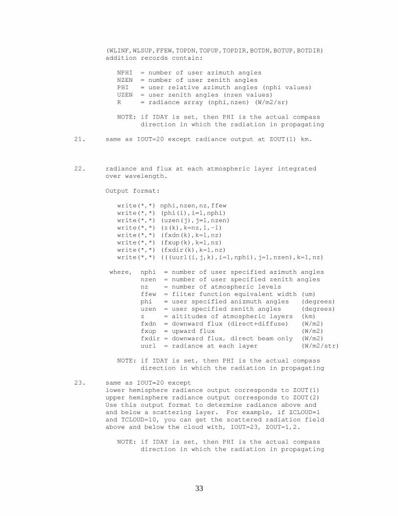
& (fdifd(i),i=1,nz), ; downward diffuse flux (w/m2/um) & (flxdn(i),i=1,nz), ; total downward flux (w/m2/um) & (flxup(i),i=1,nz) ; total upward flux (w/m2/um) enddo 10. one output record per run, integrated over wavelength. output quantities are, (integrations by trapezoid rule) WLINF,WLSUP,FFEW,TOPDN,TOPUP,TOPDIR,BOTDN,BOTUP,BOTDIR WLINF = lower wavelength limit (microns) WLSUP = upper wavelength limit (microns) FFEW = filter function equivalent width (microns) TOPDN = total downward flux at ZOUT(2) km (w/m2) TOPUP = total upward flux at ZOUT(2) km (w/m2) TOPDIR= direct downward flux at ZOUT(2) km (w/m2) BOTDN = total downward flux at ZOUT(1) km (w/m2) BOTUP = total upward flux at ZOUT(1) km (w/m2) BOTDIR= direct downward flux at ZOUT(1) km (w/m2) NOTE: To get the spectral flux density (w/m2/micron) divide any of these quantities by FFEW 11. radiant fluxes at each atmospheric layer integrated over wavelength. Output format: write(*,*) nz,phidw do i=1,nz write(*,*) zz,pp,fxdn(i),fxup(i),fxdir(i),dfdz,heat enddo where, nz = number of atmospheric layers phidw = filter function equivalent width(um) zz = level altitudes (km) pp = level pressure (mb) fxdn = downward flux (direct+diffuse) (W/m2) fxup = upward flux (W/m2) fxdir = downward flux, direct beam only (W/m2) dfdz = radiant energy flux divergence (mW/m3) heat = heating rate (K/day) NOTE: dfdz(i) and heat(i) are defined at the layer centers, i.e., halfway between level i-1 and level i. 20. radiance output at ZOUT(2) km. Output format: write(*,*) wlinf,wlsup,ffew,topdn,topup,topdir, & botdn,botup,botdir write(*,*) nphi,nzen write(*,*) (phi(i),i=1,nphi) write(*,*) (uzen(j),j=1,nzen) write(*,*) ((r(i,j),i=1,nphi),j=1,nzen) The first record of output is the same as format IOUT=10

33

(WLINF,WLSUP,FFEW,TOPDN,TOPUP,TOPDIR,BOTDN,BOTUP,BOTDIR) addition records contain: NPHI = number of user azimuth angles NZEN = number of user zenith angles PHI = user relative azimuth angles (nphi values) UZEN = user zenith angles (nzen values) R = radiance array (nphi,nzen) (W/m2/sr) NOTE: if IDAY is set, then PHI is the actual compass direction in which the radiation in propagating 21. same as IOUT=20 except radiance output at ZOUT(1) km. 22. radiance and flux at each atmospheric layer integrated over wavelength. Output format: write(*,*) nphi,nzen,nz,ffew write(*,*) (phi(i),i=1,nphi) write(*,*) (uzen(j),j=1,nzen) write(*,*) (z(k),k=nz,1,-1) write(*,*) (fxdn(k),k=1,nz) write(*,*) (fxup(k),k=1,nz) write(*,*) (fxdir(k),k=1,nz) write(*,*) (((uurl(i,j,k),i=1,nphi),j=1,nzen),k=1,nz) where, nphi = number of user specified azimuth angles nzen = number of user specified zenith angles nz = number of atmospheric levels ffew = filter function equivalent width (um) phi = user specified anizmuth angles (degrees) uzen = user specified zenith angles (degrees) z = altitudes of atmospheric layers (km) fxdn = downward flux (direct+diffuse) (W/m2) fxup = upward flux (W/m2) fxdir = downward flux, direct beam only (W/m2) uurl = radiance at each layer (W/m2/str) NOTE: if IDAY is set, then PHI is the actual compass direction in which the radiation in propagating 23. same as IOUT=20 except lower hemisphere radiance output corresponds to ZOUT(1) upper hemisphere radiance output corresponds to ZOUT(2) Use this output format to determine radiance above and and below a scattering layer. For example, if ZCLOUD=1 and TCLOUD=10, you can get the scattered radiation field above and below the cloud with, IOUT=23, ZOUT=1,2. NOTE: if IDAY is set, then PHI is the actual compass direction in which the radiation in propagating

34

========================================================================== DISORT options ============== DELTAM: if set to true, use delta-m method (see Wiscombe, 1977). This method is essentially a delta-Eddington approximation applied to multiple radiation streams. In general, for a given number of streams, intensities and fluxes will be more accurate for phase functions with a large forward peak if 'DELTAM' is set TRUE. Intensities within 10 degrees or so of the forward scattering direction will often be less accurate, however, so when primary interest centers in this so-called 'aureole region', DELTAM should be set FALSE.(default=true) NSTR: number of computational zenith angles used. NSTR must be divisible by 2. Using NSTR=4 reduces the time required for flux calculations by about a factor of 5 compared to NSTR=16, with very little penalty in accuracy (about 0.5% difference when DELTAM is set true). More streams should be used with radiance calculations. The default of NSTR depends on the value of IOUT. The default for flux computations (IOUT=1,7,10,11) is NSTR=4. The default for radiance computations (IOUT=5,6,20,21,22,23) is NSTR=20. CORINT: When set TRUE, intensities are correct for delta-M scaling effects (see Nakajima and Tanaka, 1988). When FALSE, intensities are not corrected. In general, CORINT should be set true when a beam source is present (FBEAM is not zero), DELTAM is TRUE, and the problem includes scattering. However, CORINT=FALSE runs faster and produces fairly accurate intensities outside the aureole. If CORINT=TRUE and phase function moments are specified with PMAER (IAER=5), or in aerosol.dat (IAER=-1), it is important to specify a sufficient number of phase function moments to adequately model single scattered radiation in the forward direction. Otherwise, if too few moments are provided, the intensities might actually be more accurate with CORINT=FALSE. Default value CORINT=.false. The input value of CORINT is ignored for: 1) in irradiance mode, i.e., iout ne (5,6,20,21,22) 2) there is no beam source (FBEAM=0.0), or 3) there is no scattering (SSALB=0.0 for all layers) Radiance output ===============

35

NZEN: Number of user zenith angles. If this parameter is specified SBDART will output radiance values at NZEN zenith angles, evenly spaced between the first two values of input array UZEN. For example, nzen=9, uzen=0,80 will cause output at zenith angles 0,10,20,30,40,50,60,70,80. UZEN: User zenith angles. If NZEN is specified then UZEN is interpreted as the limits of the zenith angle range, and only the first two elements are required. If NZEN is not specified then up to NSTR values of UZEN may be specified. If neither NZEN nor UZEN is specified and a radiance calculation is requested (IOUT=5,6,20,21,22,23) a default set of zenith angles is used, which depends on the value IOUT as follows: * IOUT=5 or 20: NZEN=18, UZEN=0,85 * IOUT=6 or 21: NZEN=18, UZEN=95,180 * IOUT=22 or 23: NZEN=18, UZEN=0,180 NOTE: UZEN specifies the zenith angle of at which the radiation is propagating: UZEN = 0 => radiation propagates directly up UZEN < 90 => radiation in upper hemisphere UZEN > 90 => radiation in lower hemisphere UZEN = 180 => radiation propagates directly down VZEN: user nadir angles. This is just an alternate way to specify the direction of user radiance angles, whereby uzen=180-vzen NPHI: Number of user azimuth angles. If this parameter is specified SBDART will output radiance values at NPHI azimuth angles, evenly spaced between the first two values of input array PHI. For example, nphi=7, phi=0,180 will cause output at zenith angles 0,30,60,90,120,150,180 PHI: User relative azimuth angles. If NPHI is specified then PHI is interpreted as the limits of the azimuth angle range, and only the first two elements are required. If NPHI is not specified then up to NSTR values of PHI may be specified. If neither NPHI nor PHI is specified and a radiance calculation is requested (IOUT=5,6,20,21,22,23) a default set of azimuth angles is used, equivalent to the case NPHI=19, PHI=0,180. NOTE: If SAZA is set, then PHI=0 represents radiation propagating in the Northern direction. PHI increases clockwise looking down on the Earth's surface. If SAZA is not set, then PHI is the relative azimuth angle from the forward scattering direction.

36

* PHI < 90 => forward scattered radiation * PHI > 90 => backward scattered radiation For example, if the sun is setting in the West, radiation propagating to the South-East has a relative azimuth of 45 degrees. NOTE: SBDART is currently configured to model radiation with at most 40 computational zenith angles and 40 azimuthal modes. While these limits may be expanded, be aware that running SBDART with a much larger number will significantly increase running time and memory requirements. In tests performed on a DEC Alpha, the execution time scaled roughly with NSTR^2, for NSTR less than 40. The code's memory usage also scales roughly as NSTR^2. NOTE: The default value of the solar azimuth angle, SAZA=180. This value of SAZA will cause forward scattered solar radiation to appear near PHI=0. radiation boundary conditions ============================= IBCND: = 0 : general case: boundary conditions any combination of: * beam illumination from the top ( see FBEAM) * isotropic illumination from the top ( see FISOT) * thermal emission from the top ( see TEMIS,TTEMP) * internal thermal emission sources ( see TEMPER) * reflection at the bottom ( see LAMBER,ALBEDO,HL) * thermal emission from the bottom ( see BTEMP) = 1 : isotropic illumination from top and bottom, in order to get ALBEDO and transmissivity of the entire medium vs. incident beam angle; The only input variables considered in this case are NLYR,DTAUC,SSALB,PMOM,NSTR,USRANG,NUMU,UMU,ALBEDO,DELTAM, PRNT,HEADER, and the array dimensions. NOPLNK,LAMBER are assumed TRUE, the bottom boundary can have any ALBEDO. the sole output is ALBMED,TRNMED. UMU is interpreted as the array of beam angles in this case. If USRANG = TRUE they must be positive and in increasing order, and will be returned this way; internally, however, the negatives of the UMU's are added, so MAXUMU must be at least 2*NUMU. If USRANG = FALSE, UMU is returned as the NSTR/2 positive quadrature angle cosines, in increasing order. FISOT: intensity of top-boundary isotropic illumination. (units w/sq m if thermal sources active, otherwise arbitrary units). corresponding incident flux is pi (3.14159...) times 'FISOT'.

37

TEMIS: emissivity of top layer, not used if NOTHRM=1 BTEMP: Surface (skin) temperature in Kelvin. If not set, the surface temperature is set to the temperature of the bottom layer of the model atmosphere. The surface emissivity is calculated from the albedo (see ISALB and ALBCON). The input value of BTEMP is ignored when NOTHRM=1. When SPOWDER=.true. BTEMP specifies the skin temperature of the level just below the granular layer. DISORT specific output options: =================================== PRNT(k): k 1 input variables (except PMOM) 2 fluxes 3 intensities at user levels and angles 4 planar transmissivity and planar albedo as a function solar zenith angle ( IBCND = 1 ) 5 phase function moments PMOM for each layer ( only if PRNT(1) = TRUE, and only for layers with scattering ) =========================================================================