User Guide for the Discrete DipoleApproximation Code DDSCAT 7.3

Bruce T. DrainePrinceton University Observatory

Princeton NJ 08544-1001(draine@astro.princeton.edu)

and

Piotr J. FlatauUniversity of California San Diego

Scripps Institution of OceanographyLa Jolla CA 92093-0221(pflatau@ucsd.edu)

last revised: 2013 May 26

Abstract

DDSCAT 7.3 is a freely available open-source Fortran-90 software package applying the “discretedipole approximation” (DDA) to calculate scattering and absorption of electromagnetic waves by targetswith arbitrary geometries and complex refractive index. The targets may be isolated entities (e.g., dustparticles), but may also be 1-d or 2-d periodic arrays of “target unit cells”, which can be used to studyabsorption, scattering, and electric fields around arrays of nanostructures.

The DDA approximates the target by an array of polarizable points. The theory of the DDA and itsimplementation in DDSCAT is presented in Draine (1988) and Draine & Flatau (1994), and its extensionto periodic structures in Draine & Flatau (2008). Efficient near-field calculations are carried out asdescribed in Flatau & Draine (2012). DDSCAT 7.3 allows accurate calculations of electromagneticscattering from targets with “size parameters” 2πaeff/λ <∼ 25 provided the refractive index m is notlarge compared to unity (|m − 1| <∼ 2). DDSCAT 7.3 includes support for MPI, OpenMP, and theIntel R© Math Kernel Library (MKL).

DDSCAT supports calculations for a variety of target geometries (e.g., ellipsoids, regular tetrahedra,rectangular solids, finite cylinders, hexagonal prisms, etc.). Target materials may be both inhomoge-neous and anisotropic. It is straightforward for the user to “import” arbitrary target geometries into thecode. DDSCAT automatically calculates total cross sections for absorption and scattering and selectedelements of the Mueller scattering intensity matrix for specified orientation of the target relative to theincident wave, and for specified scattering directions. DDSCAT 7.3 can calculate scattering and absorp-tion by targets that are periodic in one or two dimensions. DDSCAT 7.3 can calculate and store E and Bthroughout a user-specified rectangular volume containing the target. A Fortran-90 code ddpostprocessto support postprocessing of P, and nearfield E and B, is included in the distribution.

DDSCAT 7.3 differs from DDSCAT 7.2 by offering two new options: (1) The “Filtered CoupledDipole” method (Piller & Martin 1998; Gay-Balmaz & Martin 2002) for DDA calculations. (2) Fast near-field calculations of B. In addition, a new postprocessing code DDPOSTPROCESS.f90 is providedthat is well-documented, and much more easily modifiable by the user. As distributed, ddpostprocesscalculates the Poynting vector.

This User Guide explains how to use DDSCAT 7.3 (release 7.3.0) to carry out electromagneticscattering calculations. If you publish results calculated using DDSCAT 7.3, please cite relevant pub-lications describing the methods, e.g., Draine & Flatau (1994), Draine & Flatau (2008), and Flatau &Draine (2012).

1

arX

iv:1

305.

6497

v1 [

phys

ics.

com

p-ph

] 2

6 M

ay 2

013

CONTENTS 2

Contents1 Introduction 7

2 Applicability of the DDA 8

3 DDSCAT 7.3 123.1 What Does It Calculate? . . . . . . . . . . . . . . . . . . . . . . . . . . . . . . . . . . 12

3.1.1 Absorption and Scattering by Finite Targets . . . . . . . . . . . . . . . . . . . . 123.1.2 Absorption and Scattering by Periodic Arrays of Finite Structures . . . . . . . . 12

3.2 Application to Targets in Dielectric Media . . . . . . . . . . . . . . . . . . . . . . . . . 12

4 What’s New? 13

5 Downloading the Source Code and Example Calculations 15

6 Compiling and Linking on Unix/Linux Systems 156.1 The default Makefile . . . . . . . . . . . . . . . . . . . . . . . . . . . . . . . . . . . . 156.2 Optimization . . . . . . . . . . . . . . . . . . . . . . . . . . . . . . . . . . . . . . . . 166.3 Single vs. Double Precision . . . . . . . . . . . . . . . . . . . . . . . . . . . . . . . . 166.4 OpenMP . . . . . . . . . . . . . . . . . . . . . . . . . . . . . . . . . . . . . . . . . . 176.5 MKL: the Intel R© Math Kernel Library . . . . . . . . . . . . . . . . . . . . . . . . . . 176.6 MPI: Message Passing Interface . . . . . . . . . . . . . . . . . . . . . . . . . . . . . . 186.7 Device Numbers IDVOUT and IDVERR . . . . . . . . . . . . . . . . . . . . . . . . . 18

7 Information for Windows Users 187.1 Native executable . . . . . . . . . . . . . . . . . . . . . . . . . . . . . . . . . . . . . . 197.2 Compilation using MINGW . . . . . . . . . . . . . . . . . . . . . . . . . . . . . . . . 197.3 Compilation using CYGWIN . . . . . . . . . . . . . . . . . . . . . . . . . . . . . . . . 207.4 UBUNTU and Virtualbox . . . . . . . . . . . . . . . . . . . . . . . . . . . . . . . . . . 207.5 Compilation in Windows . . . . . . . . . . . . . . . . . . . . . . . . . . . . . . . . . . 20

8 A Sample Calculation: RCTGLPRSM 20

9 The Parameter File ddscat.par 219.1 Preliminaries . . . . . . . . . . . . . . . . . . . . . . . . . . . . . . . . . . . . . . . . 219.2 Initial Memory Allocation . . . . . . . . . . . . . . . . . . . . . . . . . . . . . . . . . 229.3 Target Geometry and Composition . . . . . . . . . . . . . . . . . . . . . . . . . . . . . 229.4 Additional Nearfield Calculation? . . . . . . . . . . . . . . . . . . . . . . . . . . . . . 229.5 Error Tolerance . . . . . . . . . . . . . . . . . . . . . . . . . . . . . . . . . . . . . . . 229.6 Maximum Number of Iterations . . . . . . . . . . . . . . . . . . . . . . . . . . . . . . 239.7 Interaction Cutoff Parameter for PBC Calculations . . . . . . . . . . . . . . . . . . . . 239.8 Angular Resolution for Computation of 〈cos θ〉, etc. . . . . . . . . . . . . . . . . . . . 239.9 Vacuum Wavelengths . . . . . . . . . . . . . . . . . . . . . . . . . . . . . . . . . . . . 239.10 Refractive Index of Ambient Medium, mmedium . . . . . . . . . . . . . . . . . . . . . 239.11 Target Size aeff . . . . . . . . . . . . . . . . . . . . . . . . . . . . . . . . . . . . . . . 249.12 Incident Polarization . . . . . . . . . . . . . . . . . . . . . . . . . . . . . . . . . . . . 249.13 Target Orientation . . . . . . . . . . . . . . . . . . . . . . . . . . . . . . . . . . . . . 249.14 Starting Values of IWAV, IRAD, IORI . . . . . . . . . . . . . . . . . . . . . . . . . . 249.15 Which Mueller Matrix Elements? . . . . . . . . . . . . . . . . . . . . . . . . . . . . . 259.16 What Scattering Directions? . . . . . . . . . . . . . . . . . . . . . . . . . . . . . . . . 25

9.16.1 Isolated Finite Targets . . . . . . . . . . . . . . . . . . . . . . . . . . . . . . . 259.16.2 1-D Periodic Targets . . . . . . . . . . . . . . . . . . . . . . . . . . . . . . . . 259.16.3 2-D Periodic Targets . . . . . . . . . . . . . . . . . . . . . . . . . . . . . . . . 25

CONTENTS 3

10 Running DDSCAT 7.3 Using the Sample ddscat.par File 2510.1 Single-Process Execution . . . . . . . . . . . . . . . . . . . . . . . . . . . . . . . . . 2510.2 Code Execution Under MPI . . . . . . . . . . . . . . . . . . . . . . . . . . . . . . . . 26

11 Output Files 2711.1 ASCII files . . . . . . . . . . . . . . . . . . . . . . . . . . . . . . . . . . . . . . . . . 2711.2 Binary Option . . . . . . . . . . . . . . . . . . . . . . . . . . . . . . . . . . . . . . . 28

12 Choice of Iterative Algorithm 28

13 Choice of FFT Algorithm 29

14 Choice of DDA Method 3014.1 Point Dipoles: Options LATTDR and GKDLDR . . . . . . . . . . . . . . . . . . . . . . 3014.2 Filtered Coupled Dipole: option FLTRCD . . . . . . . . . . . . . . . . . . . . . . . . . 31

15 Dielectric Functions 31

16 Calculation of 〈cos θ〉, Radiative Force, and Radiation Torque 33

17 Memory Requirements 33

18 Target Geometry: The Target Frame 34

19 Target Orientation 3419.1 Orientation of the Target in the Lab Frame . . . . . . . . . . . . . . . . . . . . . . . . 3419.2 Orientation of the Incident Beam in the Target Frame . . . . . . . . . . . . . . . . . . . 3619.3 Sampling in Θ, Φ, and β . . . . . . . . . . . . . . . . . . . . . . . . . . . . . . . . . . 36

20 Orientational Averaging 3720.1 Randomly-Oriented Targets . . . . . . . . . . . . . . . . . . . . . . . . . . . . . . . . 3720.2 Nonrandomly-Oriented Targets . . . . . . . . . . . . . . . . . . . . . . . . . . . . . . 37

21 Target Generation: Isolated Finite Targets 3821.1 FROM_FILE = Target composed of possibly anisotropic material, defined by list of

dipole locations and “compositions” obtained from a file . . . . . . . . . . . . . . . . . 3921.1.1 Sample calculation in directory examples_exp/FROM_FILE . . . . . . . . . 40

21.2 ANIFRMFIL = General anistropic target defined by list of dipole locations,“compositions”,and material orientations obtained from a file . . . . . . . . . . . . . . . . . . . . . . . 40

21.3 ANIELLIPS = Homogeneous, anisotropic ellipsoid. . . . . . . . . . . . . . . . . . . . 4221.4 ANI_ELL_2 = Two touching, homogeneous, anisotropic ellipsoids, with distinct com-

positions . . . . . . . . . . . . . . . . . . . . . . . . . . . . . . . . . . . . . . . . . . 4221.5 ANI_ELL_3 = Three touching homogeneous, anisotropic ellipsoids with same size and

orientation but distinct dielectric tensors . . . . . . . . . . . . . . . . . . . . . . . . . . 4221.6 ANIRCTNGL = Homogeneous, anisotropic, rectangular solid . . . . . . . . . . . . . . 42

21.6.1 Sample calculation in directory examples_exp/ANIRCTNGL . . . . . . . . . 4221.7 CONELLIPS = Two concentric ellipsoids . . . . . . . . . . . . . . . . . . . . . . . . . 4321.8 CYLINDER1 = Homogeneous, isotropic finite cylinder . . . . . . . . . . . . . . . . . 4421.9 CYLNDRCAP = Homogeneous, isotropic finite cylinder with hemispherical endcaps. . 4421.10 DSKRCTNGL = Disk on top of a homogeneous rectangular slab . . . . . . . . . . . . 4421.11 DW1996TAR = 13 block target used by Draine & Weingartner (1996). . . . . . . . . . 4521.12 ELLIPSOID = Homogeneous, isotropic ellipsoid. . . . . . . . . . . . . . . . . . . . . 45

21.12.1 Sample calculation in directory examples_exp/ELLIPSOID . . . . . . . . . 4521.12.2 Sample calculation in directory examples_exp/ELLIPSOID_NEARFIELD . 45

21.13 ELLIPSO_2 = Two touching, homogeneous, isotropic ellipsoids, with distinct compo-sitions . . . . . . . . . . . . . . . . . . . . . . . . . . . . . . . . . . . . . . . . . . . . 46

CONTENTS 4

21.14 ELLIPSO_3 = Three touching homogeneous, isotropic ellipsoids of equal size and ori-entation, but distinct compositions . . . . . . . . . . . . . . . . . . . . . . . . . . . . . 46

21.15 HEX_PRISM = Homogeneous, isotropic hexagonal prism . . . . . . . . . . . . . . . . 4621.16 LAYRDSLAB = Multilayer rectangular slab . . . . . . . . . . . . . . . . . . . . . . . 4721.17 MLTBLOCKS = Homogeneous target constructed from cubic “blocks” . . . . . . . . . 4721.18 RCTGLPRSM = Homogeneous, isotropic, rectangular solid . . . . . . . . . . . . . . . 47

21.18.1 Sample calculation in directory examples_exp/RCTGLPRSM . . . . . . . . 4721.18.2 Sample calculation in directory examples_exp/RCTGLPRSM_NEARFIELD 48

21.19 RCTGLBLK3 = Stack of 3 rectangular blocks, with centers on the xTF axis. . . . . . . 4821.20 SLAB_HOLE = Rectangular slab with a cylindrical hole. . . . . . . . . . . . . . . . . 4821.21 SPHERES_N = Multisphere target = union of N spheres of single isotropic material . . 48

21.21.1 Sample calculation in directory examples_exp/SPHERES_N . . . . . . . . . 4921.22 SPHROID_2 = Two touching homogeneous, isotropic spheroids, with distinct compo-

sitions . . . . . . . . . . . . . . . . . . . . . . . . . . . . . . . . . . . . . . . . . . . . 4921.23 SPH_ANI_N = Multisphere target consisting of the union of N spheres of various ma-

terials, possibly anisotropic . . . . . . . . . . . . . . . . . . . . . . . . . . . . . . . . 5021.23.1 Sample calculation in directory examples_exp/SPH_ANI_N . . . . . . . . . 51

21.24 TETRAHDRN = Homogeneous, isotropic tetrahedron . . . . . . . . . . . . . . . . . . 5121.25 TRNGLPRSM = Triangular prism of homogeneous, isotropic material . . . . . . . . . 5121.26 UNIAXICYL = Homogeneous finite cylinder with uniaxial anisotropic dielectric tensor 5121.27 Modifying Existing Routines or Writing New Ones . . . . . . . . . . . . . . . . . . . . 5121.28 Testing Target Generation using CALLTARGET . . . . . . . . . . . . . . . . . . . . . 51

22 Target Generation: Periodic Targets 5222.1 FRMFILPBC = periodic target with TUC geometry and composition input from a file . 52

22.1.1 Sample calculation in directory examples_exp/FRMFILPBC . . . . . . . . . 5322.2 ANIFILPBC = general anisotropic periodic target with TUC geometry and composition

input from a file . . . . . . . . . . . . . . . . . . . . . . . . . . . . . . . . . . . . . . 5322.3 BISLINPBC = Bi-Layer Slab with Parallel Lines . . . . . . . . . . . . . . . . . . . . . 5322.4 CYLNDRPBC = Target consisting of homogeneous cylinder repeated in target y and/or

z directions using periodic boundary conditions . . . . . . . . . . . . . . . . . . . . . . 5422.4.1 Sample calculation in directory examples_exp/CYLNDRPBC . . . . . . . . 55

22.5 DSKBLYPBC = Target consisting of a periodic array of disks on top of a two-layerrectangular slabs. . . . . . . . . . . . . . . . . . . . . . . . . . . . . . . . . . . . . . . 55

22.6 DSKRCTPBC = Target consisting of homogeneous rectangular brick plus a disk, ex-tended in target y and z directions using periodic boundary conditions . . . . . . . . . . 5622.6.1 Sample calculation in directory examples_exp/DSKRCTPBC . . . . . . . . . 57

22.7 HEXGONPBC = Target consisting of homogeneous hexagonal prism repeated in targety and/or z directions using periodic boundary conditions . . . . . . . . . . . . . . . . . 57

22.8 LYRSLBPBC = Target consisting of layered slab, extended in target y and z directionsusing periodic boundary conditions . . . . . . . . . . . . . . . . . . . . . . . . . . . . . 59

22.9 RCTGL_PBC = Target consisting of homogeneous rectangular brick, extended in targety and z directions using periodic boundary conditions . . . . . . . . . . . . . . . . . . . 6122.9.1 Sample calculation in directory examples_exp/RCTGL_PBC . . . . . . . . . 6122.9.2 Sample calculation in directory examples_exp/RCTGL_PBC_NEARFIELD 6122.9.3 Sample calculation in directory examples_exp/RCTGL_PBC_NEARFLD_B 61

22.10 RECRECPBC = Rectangular solid resting on top of another rectangular solid, repeatedperiodically in target y and z directions using periodic boundary conditions . . . . . . . 63

22.11 SLBHOLPBC = Target consisting of a periodic array of rectangular blocks, each con-taining a cylindrical hole . . . . . . . . . . . . . . . . . . . . . . . . . . . . . . . . . . 65

22.12 SPHRN_PBC = Target consisting of group of N spheres, extended in target y and zdirections using periodic boundary conditions . . . . . . . . . . . . . . . . . . . . . . . 6522.12.1 Sample calculation in directory examples_exp/SPHRN_PBC . . . . . . . . . 66

22.13 TRILYRPBC = Three stacked rectangular blocks, repeated periodically . . . . . . . . . 66

CONTENTS 5

23 Scattering Directions 6723.1 Isolated Finite Targets . . . . . . . . . . . . . . . . . . . . . . . . . . . . . . . . . . . 6723.2 Scattering Directions for Targets that are Periodic in 1 Dimension . . . . . . . . . . . . 6723.3 Scattering Directions for Targets for Doubly-Periodic Targets . . . . . . . . . . . . . . 69

24 Incident Polarization State 70

25 Averaging over Scattering Directions: g(1) = 〈cos θs〉, etc. 7025.1 Angular Averaging . . . . . . . . . . . . . . . . . . . . . . . . . . . . . . . . . . . . . 7025.2 Selection of Scattering Angles θs, φs . . . . . . . . . . . . . . . . . . . . . . . . . . . . 7225.3 Accuracy of Angular Averaging as a Function of η . . . . . . . . . . . . . . . . . . . . 73

26 Scattering by Finite Targets: The Mueller Matrix 7426.1 Two Orthogonal Incident Polarizations (IORTH=2) . . . . . . . . . . . . . . . . . . . . 7426.2 Stokes Parameters . . . . . . . . . . . . . . . . . . . . . . . . . . . . . . . . . . . . . 7526.3 Relation Between Stokes Parameters of Incident and Scattered Radiation: The Mueller

Matrix . . . . . . . . . . . . . . . . . . . . . . . . . . . . . . . . . . . . . . . . . . . . 7626.4 Polarization Properties of the Scattered Radiation . . . . . . . . . . . . . . . . . . . . . 7626.5 Relation Between Mueller Matrix and Scattering Cross Sections . . . . . . . . . . . . . 7726.6 One Incident Polarization State Only (IORTH=1) . . . . . . . . . . . . . . . . . . . . . 78

27 Scattering by Periodic Targets: Generalized Mueller Matrix 7927.1 Mueller Matrix S(1d)

ij for Targets Periodic in One Direction . . . . . . . . . . . . . . . . 79

27.2 Mueller Matrix S(2d)ij (M,N) for Targets Periodic in Two Directions . . . . . . . . . . . 79

28 Composite Targets with Anisotropic Constituents 79

29 Near-Field Calculations: E and B Within or Near the Target 8129.1 Running DDSCAT 7.3 with NRFLD = 1 . . . . . . . . . . . . . . . . . . . . . . . . . . 8129.2 Running DDSCAT 7.3 with NRFLD = 2 . . . . . . . . . . . . . . . . . . . . . . . . . . 8229.3 The Binary Files wxxxryyykzzz.En . . . . . . . . . . . . . . . . . . . . . . . . . . . . 8229.4 The Binary Files wxxxryyykzzz.EBn . . . . . . . . . . . . . . . . . . . . . . . . . . . . 82

30 Post-Processing of Near-Field Calculations 8330.1 The Program ddpostprocess . . . . . . . . . . . . . . . . . . . . . . . . . . . . . . . . 8330.2 Modifying DDPOSTPROCESS.f90 . . . . . . . . . . . . . . . . . . . . . . . . . . . . 85

31 Displaying Target Shapes 8631.1 VTRCONVERT . . . . . . . . . . . . . . . . . . . . . . . . . . . . . . . . . . . . . . . 8631.2 What is VTK? . . . . . . . . . . . . . . . . . . . . . . . . . . . . . . . . . . . . . . . 8631.3 How to plot shapes once you have VTR/PVD files. . . . . . . . . . . . . . . . . . . . . 86

32 Visualization of the Electric Field 88

33 Finale 89

34 Acknowledgments 90

A Understanding and Modifying ddscat.par 93

B wxxxryyy.avg Files 95

C wxxxryyykzzz.sca Files 97

D wxxxryyykzzz.poln Files 99

CONTENTS 6

E wxxxryyykzzz.En Files 99

F wxxxryyykzzz.EBn Files 99

Index 100

1 INTRODUCTION 7

1 IntroductionDDSCAT is a software package to calculate scattering and absorption of electromagnetic waves by tar-gets with arbitrary geometries using the “discrete dipole approximation” (DDA). In this approximationthe target is replaced by an array of point dipoles (or, more precisely, polarizable points); the electromag-netic scattering problem for an incident periodic wave interacting with this array of point dipoles is thensolved essentially exactly. The DDA (sometimes referred to as the “coupled dipole approximation”) wasapparently first proposed by Purcell & Pennypacker (1973). DDA theory was reviewed and developedfurther by Draine (1988), Draine & Goodman (1993), reviewed by Draine & Flatau (1994), and recentlyextended to periodic structures by Draine & Flatau (2008).

DDSCAT 7.3, the current release of DDSCAT, is an open-source Fortran 90 implementation of theDDA developed by the authors.1 DDSCAT 7.3 calculates absorption and scattering by isolated targets, ortargets that are periodic in one or two dimensions, using methods described by Draine & Flatau (2008).

DDSCAT is intended to be a versatile tool, suitable for a wide variety of applications includingstudies of interstellar dust, atmospheric aerosols, blood cells, marine microorganisms, and nanostructurearrays. As provided, DDSCAT 7.3 should be usable for many applications without modification, but theprogram is written in a modular form, so that modifications, if required, should be fairly straightforward.

The authors make this code openly available to others, in the hope that it will prove a useful tool. Weask only that:

• If you publish results obtained using DDSCAT, please acknowledge the source of the code, andcite relevant papers, such as Draine (1988), Goodman et al. (1990), Draine & Flatau (1994), Draine& Flatau (2008), and Flatau & Draine (2012).

• If you discover any errors in the code or documentation, please promptly communicate them to theauthors.

• You comply with the “copyleft" agreement (more formally, the GNU General Public License) ofthe Free Software Foundation: you may copy, distribute, and/or modify the software identified ascoming under this agreement. If you distribute copies of this software, you must give the recipientsall the rights which you have. See the file doc/copyleft.txt distributed with the DDSCATsoftware.

We also strongly encourage you to send email to draine@astro.princeton.edu identifyingyourself as a user of DDSCAT; this will enable the authors to notify you of any bugs, corrections, orimprovements in DDSCAT. Up-to-date information on DDSCAT and the latest version of DDSCAT 7.3can be found at

http://code.google.com/p/ddscat/

1 The release history of DDSCAT is as follows:• DDSCAT 4b: Released 1993 March 12• DDSCAT 4b1: Released 1993 July 9• DDSCAT 4c: Although never announced, DDSCAT.4c was made available to a number of interested users beginning 1994

December 18• DDSCAT 5a7: Released 1996• DDSCAT 5a8: Released 1997 April 24• DDSCAT 5a9: Released 1998 December 15• DDSCAT 5a10: Released 2000 June 15• DDSCAT 6.0: Released 2003 September 2• DDSCAT 6.1: Released 2004 September 10• DDSCAT 7.0: Released 2008 September 1• DDSCAT 7.1: Released 2010 February 7• DDSCAT 7.2: Released 2012 February 15• DDSCAT 7.2.1: Released 2012 May 14• DDSCAT 7.2.2: Released 2012 June 3• DDSCAT 7.3.0: Released 2013 May 26

2 APPLICABILITY OF THE DDA 8

The current version, DDSCAT 7.3, offers the option of using the DDA formulae from Draine (1988),with dipole polarizabilities determined from the Lattice Dispersion Relation (Draine & Goodman 1993;Gutkowicz-Krusin & Draine 2004). Alternatively, DDSCAT 7.3 also allows the user to specify the“filtered coupled dipole” method of Piller & Martin (1998) and Gay-Balmaz & Martin (2002), whichmay give better results for targets with “large” refractive indices |m− 1| >∼ 2.

The code incorporates Fast Fourier Transform (FFT) methods (Goodman et al. 1990). DDSCAT7.3 includes capability to calculate scattering and absorption by targets that are periodic in one or twodimensions – arrays of nanostructures, for example. The theoretical basis for application of the DDAto periodic structures is developed in Draine & Flatau (2008). DDSCAT 7.3 includes capability toefficiently perform “nearfield” calculations of E and B in and around the target using FFT methods, asdescribed by Flatau & Draine (2012). A new postprocessing code, DDPOSTPROCESS.f90, is includedin the DDSCAT 7.3 distribution.

We refer you to the list of references at the end of this document for discussions of the theoryand accuracy of the DDA [in particular, reviews by Draine & Flatau (1994) and Draine (2000), recentextension to 1-d and 2-d arrays by Draine & Flatau (2008), and comparison of the coupled dipole methodwith other DDA methods (including the filtered coupled dipole method) by Yurkin et al. (2010)].

In §2 we summarize the applicability of the DDA, and in §3 we describe what the current release cancalculate.

In §4 we describe the principal changes between DDSCAT 7.3 and the previous releases. The suc-ceeding sections contain instructions for:

• obtaining the source code (§5);

• compiling and linking the code (§6);

• information for Microsoft R© Windows users (§7);

• running a sample calculation (§8);

• modifying the parameter file to do your desired calculations (§9);

• specifying target orientation(s) (§19);

• understanding the output from the sample calculation;

• using DDPOSTPROCESS.f90 for postprocessing of solutions found by DDSCAT 7.3 (§30.1).

The instructions for compiling, linking, and running will be appropriate for a Linux system; slightchanges will be necessary for non-Linux sites, but they are quite minor and should present no difficulty.

Finally, the current version of this User Guide can be obtained fromhttp://arxiv.org/abs/xxxx.xxxx.

Important Note: DDSCAT 7.3 differs in a number of respects from previous versions of DDSCAT.DDSCAT 7.3 includes support for both MPI and OpenMP, but – as of this writing – DDSCAT 7.3 hasnot yet been tested with MPI, and there has been only limited testing with OpenMP. DDSCAT 7.3 hasbeen tested extensively on single-processor systems, but if you are intending to use DDSCAT 7.3 withOpenMP or MPI, please proceed with caution – do at least a few comparison calculations in single-cpumode to verify that the results obtained with OpenMP or MPI appear to be correct. If you do encounterproblems with OpenMP or MPI, please document them and communicate them to the authors. And ifyou find that everything appears to work properly, we’d like to know that too!

2 Applicability of the DDAThe principal advantage of the DDA is that it is completely flexible regarding the geometry of the target,being limited only by the need to use an interdipole separation d small compared to (1) any structurallengths in the target, and (2) the wavelength λ. Numerical studies (Draine & Goodman 1993; Draine &Flatau 1994; Draine 2000) indicate that the second criterion is adequately satisfied if

|m|kd < 1 , (1)

2 APPLICABILITY OF THE DDA 9

wherem is the complex refractive index of the target material, and k ≡ 2π/λ, where λ is the wavelengthin vacuo. This criterion is valid provided that |m − 1| <∼ 3 or so. When Im(m) becomes large, theDDA solution tends to overestimate the absorption cross section Cabs, and it may be necessary to useinterdipole separations d smaller than indicated by eq. (1) to reduce the errors in Cabs to acceptablevalues.

If accurate calculations of the scattering phase function (e.g., radar or lidar cross sections) are desired,a more conservative criterion

|m|kd < 0.5 (2)

will usually ensure that differential scattering cross sections dCsca/dΩ are accurate to within a fewpercent of the average differential scattering cross section Csca/4π (see Draine 2000).

Let V be the actual volume of solid material in the target.2 If the target is represented by an array ofN dipoles, located on a cubic lattice with lattice spacing d, then

V = Nd3 . (3)

We characterize the size of the target by the “effective radius”

aeff ≡ (3V/4π)1/3 , (4)

the radius of an equal volume sphere. A given scattering problem is then characterized by the dimen-sionless “size parameter”

x ≡ kaeff =2πaeff

λ. (5)

The size parameter can be related to N and |m|kd:

x ≡ 2πaeff

λ=

62.04

|m|

(N

106

)1/3

· |m|kd . (6)

Equivalently, the target size can be written

aeff = 9.873λ

|m|

(N

106

)1/3

· |m|kd . (7)

Practical considerations of CPU speed and computer memory currently available on scientific worksta-tions typically limit the number of dipoles employed to N < 106 (see §17 for limitations on N due toavailable RAM); for a given N , the limitations on |m|kd translate into limitations on the ratio of targetsize to wavelength.For calculations of total cross sections Cabs and Csca, we require |m|kd < 1:

aeff < 9.88λ

|m|

(N

106

)1/3

or x <62.04

|m|

(N

106

)1/3

. (8)

For scattering phase function calculations, we require |m|kd < 0.5:

aeff < 4.94λ

|m|

(N

106

)1/3

or x <31.02

|m|

(N

106

)1/3

. (9)

It is therefore clear that the DDA is not suitable for very large values of the size parameter x, or verylarge values of the refractive index m. The primary utility of the DDA is for scattering by dielectrictargets with sizes comparable to the wavelength. As discussed by Draine & Goodman (1993), Draine& Flatau (1994), and Draine (2000), total cross sections calculated with the DDA are accurate to a fewpercent provided N > 104 dipoles are used, criterion (1) is satisfied, and the refractive index is not toolarge.

For fixed |m|kd, the accuracy of the approximation degrades with increasing |m − 1|, for reasonshaving to do with the surface polarization of the target, as discussed by Collinge & Draine (2004). Withthe present code, good accuracy can be achieved for |m− 1| < 2.

2 APPLICABILITY OF THE DDA 10

Figure 1: Scattering and absorption for a sphere with m = 1.33 + 0.01i. The upper panel shows the exact values of Qsca andQabs, obtained with Mie theory, as functions of x = ka. The middle and lower panels show fractional errors in Qsca and Qabs,obtained using DDSCAT with polarizabilities obtained from the Lattice Dispersion Relation, and labelled by the number N ofdipoles in each pseudosphere. After Fig. 1 of Draine & Flatau (1994).

Figure 2: Same as Fig. 1, but for m = 2 + i. After Fig. 2 of Draine & Flatau (1994). Note: in the upper panel, the labels forQsca,Mie and Qabs,Mie should be interchanged.

Examples illustrating the accuracy of the DDA are shown in Figs. 1–2, which show overall scatteringand absorption efficiencies as a function of wavelength for different discrete dipole approximations to asphere, with N ranging from 304 to 59728. The DDA calculations assumed radiation incident along the(1,1,1) direction in the “target frame”. Figs. 3–4 show the scattering properties calculated with the DDA

2 In the case of an infinite periodic target, V is the volume of solid material in one “Target Unit Cell”.

2 APPLICABILITY OF THE DDA 11

Figure 3: Differential scattering cross section for m = 1.33 + 0.01i pseudosphere and ka = 7. Lower panel shows fractionalerror compared to exact Mie theory result. TheN = 17904 pseudosphere has |m|kd = 0.57, and an rms fractional error in dσ/dΩof 2.4%. After Fig. 5 of Draine & Flatau (1994).

Figure 4: Same as Fig. 3 but for m = 2 + i. The N = 59728 pseudosphere has |m|kd = 0.65, and an rms fractional error indσ/dΩ of 6.7%. After Fig. 8 of Draine & Flatau (1994).

for x = ka = 7. Additional examples can be found in Draine & Flatau (1994) and Draine (2000).As discussed below, DDSCAT 7.3 can also calculate scattering and absorption by targets that are

periodic in one or two directions – for examples, see Draine & Flatau (2008).

3 DDSCAT 7.3 12

3 DDSCAT 7.3

3.1 What Does It Calculate?

3.1.1 Absorption and Scattering by Finite Targets

DDSCAT 7.3, like previous versions of DDSCAT, solves the problem of scattering and absorption bya finite target, represented by an array of polarizable point dipoles, interacting with a monochromaticplane wave incident from infinity. DDSCAT 7.3 has the capability of automatically generating dipolearray representations for a variety of target geometries (see §21) and can also accept dipole array repre-sentations of targets supplied by the user (although the dipoles must be located on a cubic lattice). Theincident plane wave can have arbitrary elliptical polarization (see §24), and the target can be arbitrarilyoriented relative to the incident radiation (see §19). The following quantities are calculated by DDSCAT7.3 :

• Absorption efficiency factor Qabs ≡ Cabs/πa2eff , where Cabs is the absorption cross section;

• Scattering efficiency factor Qsca ≡ Csca/πa2eff , where Csca is the scattering cross section;

• Extinction efficiency factor Qext ≡ Qsca +Qabs;

• Phase lag efficiency factor Qpha, defined so that the phase-lag (in radians) of a plane wave afterpropagating a distance L is just ntQphaπa

2effL, where nt is the number density of targets.

• The 4×4 Mueller scattering intensity matrix Sij describing the complete scattering properties ofthe target for scattering directions specified by the user (see §26).

• Radiation force efficiency vector Qrad (see §16).

• Radiation torque efficiency vector QΓ (see §16).

In addition, the user can choose to have DDSCAT 7.3 store the solution for post-processing.

3.1.2 Absorption and Scattering by Periodic Arrays of Finite Structures

DDSCAT 7.3 includes the capability to solve the problem of scattering and absorption by an infinitetarget consisting of a 1-d or 2-d periodic array of finite structures, illuminated by an incident plane wave.The finite structures are themselves represented by arrays of point dipoles.

The electromagnetic scattering problem for periodic arrays is formulated by Draine & Flatau (2008),who show how the problem can be reduced to a finite system of linear equations, and solved by the samemethods used for scattering by finite targets.

The far-field scattering properties of the 1-d and 2-d periodic arrays can be conveniently representedby a generalization of the Mueller scattering matrix to the 1-d or 2-d periodic geometry – see Draine &Flatau (2008) for definition of S(1d)

ij (M, ζ) and S(2d)ij (M,N). For targets with 1-d periodicity, DDSCAT

7.3 calculates S(1d)ij (M, ζ) for user-specified M and ζ. For targets with 2-d periodicity, DDSCAT 7.3

calculates S(2d)ij (M,N) for both transmission and reflection, for user-specified (M,N).

As for finite targets, the user can choose to have DDSCAT 7.3 store the calculated polarization fieldfor post-processing.

3.2 Application to Targets in Dielectric MediaLet ω be the angular frequency of the incident radiation. Beginning with DDSCAT 7.2, DDSCAT

facilitates calculation of absorption and scattering by targets immersed in dielectric media (e.g., liquidwater). In the parameter file ddscat.par, the user simply specifies the refractive index mmedium ofthe ambient medium. If the target is in vacuo, set mmedium = 1. Otherwise, set mmedium to be therefractive index in the ambient medium at frequency ω. For example, H2O has mmedium = 1.335 nearω/2π = 6 × 1014 Hz, the frequency corresponding to λvac = 500 nm (green light). At this frequency,air at STP has mmedium = 1.00028, which can be taken to be 1 for most applications.

The wavelength provided in the file ddscat.par should be the vacuum wavelength λvac = 2πc/ωcorresponding to the frequency ω.

4 WHAT’S NEW? 13

The dielectric function or refractive index for the target material is provided via a file, with thefilename provided via ddscat.par. The file should give either the actual complex dielectric functionεtarget or actual complex refractive index mtarget =

√εtarget of the target material, as a function of

wavelength in vacuo.Internal to DDSCAT 7.3, the scattering calculation is carried out using the relative dielectric function

εrel(ω) =εtarget(ω)

εmedium(ω), (10)

relative refractive index:

mrel(ω) =mtarget(ω)

mmedium(ω), (11)

and wavelength in the ambient medium

λmedium =λvac

mmedium. (12)

The absorption, scattering, extinction, and phase lag efficiency factors Qabs, Qsca, Qext, and Qpha

calculated by DDSCAT will then be equal to the physical cross sections for absorption, scattering, andextinction divided by πa2

eff . For example, the attenuation coefficient α for radiation propagating througha diffuse medium with a number density nt of scatterers will be just

α = ntQextπa2eff . (13)

Similarly, the phase lag (in radians) after propagating a distance L will be ntQphaπa2effL.

The elements Sij of the 4×4 Mueller scattering matrix S calculated by DDSCAT for finite targetswill be correct for scattering in the medium:

Isca =

(λmedium

2πr

)2

S · Iin, (14)

where Iin and Isca are the Stokes vectors for the incident and scattered light (in the medium), r is thedistance from the target, and λmedium is the wavelength in the medium (eq. 12). See §26 for a detaileddiscussion of the Mueller scattering matrix.

The time-averaged radiative force and torque (see §16) on a finite target in a dielectric medium are

Frad = Qprπa2effurad , (15)

Γrad = QΓπa2effurad

λmedium

2π, (16)

where the time-averaged energy density is

urad = εmedium|E0|2

8π, (17)

where E0 cos(ωt+ φ) is the electric field of the incident plane wave in the medium.The relationship between the microscopic and macroscopic fields Emicro and Emacro is discussed in

§29 (see eq. 129).

4 What’s New?DDSCAT 7.3 differs from DDSCAT 7.1 in several ways, including:

1. N.B.: The structure of the parameter file ddscat.par has again been changed: ddscat.parfiles that were used with DDSCAT 7.1 or DDSCAT 7.2 will need to be modified. See §9 andAppendix A.

4 WHAT’S NEW? 14

2. As in DDSCAT 7.2, DDSCAT 7.3 requires the user to specify the (real) refractive index mambient

of the ambient medium. See §9.3. As with DDSCAT 7.2, DDSCAT 7.3 includes support for two additional conjugate gradient

solvers (see §12):• GPBICG – Implementation by Chamuet and Rahmani of the Complex Conjugate Gradient

solver presented by Tang et al. (2004).• QMRCCG – Quasi-Minimum-Residual Complex Conjugate Gradient solver, adapted from

fortran-90 implementation kindly made available by P.C. Chaumet and A. Rahmani (Chaumet& Rahmani 2009).

4. As with DDSCAT 7.2, DDSCAT 7.3 requires the user to specify the maximum allowed numberof iterations (this was previously hard-wired).

5. As with DDSCAT 7.2, DDSCAT 7.3 supports fast calculations of the electric field within and nearthe target using FFT methods, as described by Flatau & Draine (2012); see §29). The programDDFIELD that came with DDSCAT 7.1 is no longer needed (and no longer supported).

6. DDSCAT 7.3 now includes the option of fast calculations of B in and near the target using FFTmethods (see §29).

7. As with DDSCAT 7.2, the DDSCAT 7.3 distribution includes a set of “example” calculations, buta new example has been added:• FROM_FILE: target whose geometry is supplied via an ascii file• ELLIPSOID: sphere, with nearfield calculation of E in and around the sphere.• RCTGLPRSM: rectangular brick• SPH_ANI_N: cluster of spheres, each characterized by an anisotropic dielectric function• CYLNDRPBC: infinite cylinder, calculated as a periodic array of disks.• DSKRCTPBC: doubly-periodic array of Au disks supported by a Si3N4 slab.• RCTGL_PBC: doubly-periodic array of rectangular blocks.• RCTGL_PBC: doubly-periodic array of rectangular blocks, with nearfield calculation of E

in and around the sphere.• SPHRN_PBC: doubly-periodic array of clusters of spheres.• ELLIPSOID_NEARFIELD: same calculation as in the ELLIPSOID example, followed by

a nearfield calculation of E in and around the sphere, followed by evaluation of E along atrack passing through the sphere, plus creation of “VTK” files for visualization.

• RCTGLPRSM_NEARFIELD: same calculation as in the RCTGLPRSM example, fol-lowed by a nearfield calculation of E in and around the target, followed by evaluation ofE along a track passing through the prism, plus creation of “VTK” files for visualization.

• RCTGL_PBC_NEARFIELD: same calculation as in the RCTGL_PBC example, followedby a nearfield calculation of E in and around the target, followed by evaluation of E along atrack passing through the prism, plus creation of “VTK” files for visualization.

• RCTGL_PBC_NEARFLD_B: same calculation as in the RCTGL_PBC_NARFIELD ex-ample, followed by evaluation of both E and B along a track passing through the prism, pluscreation of “VTK” files for visualization.

8. DDSCAT 7.3 is distributed with a program VTRCONVERT.f90 that supports visualization oftarget geometries using the Visualization Toolkit (VTK), an open-source, freely-available softwaresystem for 3D computer graphics (http://www.vtk.org) and, specifically, ParaView (http://paraview.org).

9. DDSCAT 7.3 is distributed with a program DDPOSTPROCESS.f90.• DDPOSTPROCESS.f90 allows the user to easily extract E (and B if it was also precalcu-

lated) at points along a line.• If B was precalculated, DDPOSTPROCESS.f90 calculates the time-averaged Poynting vec-

tor c〈E×H〉/4π at each point in the computational volume.• DDPOSTPROCESS.f90 creates “VTK” files for visualization of |E|, |E|2, or (c/4π)〈E ×

H〉 using the VTK tools.

5 DOWNLOADING THE SOURCE CODE AND EXAMPLE CALCULATIONS 15

5 Downloading the Source Code and Example CalculationsDDSCAT 7.3 is written in standard Fortran-90 with a single extension: it uses the Fortran-95 standardlibrary call CPU_TIME to obtain timing information. DDSCAT 7.3 is therefore portable to any systemhaving a f90 or f95 compiler. It has been successfully compiled with many different compilers, includinggfortran, g95, ifort, pgf77, and NAG R©f95.

It is possible to use DDSCAT 7.3 on PCs running Microsoft R©Windows operating systems, includingVista and Windows 7. Section 7 provides instructions for creating a unix-like environment in which youcan compile and run DDSCAT 7.3.

Alternatively, you may be able to obtain a precompiled native executable – see §7.1. More informa-tion on how to do this can be found at

http://code.google.com/p/ddscatThe remainder of this section will assume that the installation is taking place on a Unix, Linux or Mac

OSX system with the standard developer tools (e.g., tar, make, and a f90 or f95 compiler) installed.The complete source code for DDSCAT 7.3 is provided in a single gzipped tarfile. To obtain the

source code, simply point your browser to http://code.google.com/p/ddscat/ and down-load the latest release.

After downloading ddscat7.3.0.tgz into the directory where you would like DDSCAT 7.3 toreside (you should have at least 10 Mbytes of disk space available), the source code can be installed asfollows:

If you are on a Linux system, you should be able to typetar xvzf ddscat7.3.0.tgz

which will“extract” the files from the gzipped tarfile. If your version of “tar” doesn’t support the “z”option, then try

zcat ddscat7.3.0.tgz | tar xvf -If neither of the above work on your system, try the two-stage procedure

gunzip ddscat7.3.0.tgztar xvf ddscat7.3.0.tar

The only disadvantage of the two-stage procedure is that it uses more disk space, since after the secondstep you will have the uncompressed tarfile ddscat7.3.0.tar – about 3.8 Mbytes – in addition toall the files you have extracted from the tarfile – another 4.6 Mbytes.

Any of the above approaches should create subdirectories src, doc, diel, and examples_exp.

• src contains the source code.

• doc contains documentation (including this UserGuide).

• diel contains a few sample files specifying refractive indices or dielectric functions as functionsof vacuum wavelength.

It is also recommended that you download ddscat7.3.0_examples.tgz, followed bytar xvzf ddscat7.3.0_examples.tgz

Subdirectory examples_exp contains sample ddscat.par files as well as output files for variousexample problems, including both isolated targets and infinite periodic targets. It also includes sampleddpostprocess.par files for running ddpostprocess to support visualization following nearfieldcalculations.

6 Compiling and Linking on Unix/Linux SystemsIn the discussion below, it is assumed that the DDSCAT 7.3 source code has been installed in a directoryDDA/src. The instructions below assume that you are on a Unix, Linux, or Mac OSX system.

6.1 The default MakefileIt is assumed that the system has the following already installed:

• a Fortran-90 compiler (e.g., gfortran, g95, Intel R© ifort, or NAG R©f95) .

6 COMPILING AND LINKING ON UNIX/LINUX SYSTEMS 16

• cpp – the “C preprocessor”.

There are a number of different ways to create an executable, depending on what options the user wants:

• what compiler and compiler flags?

• single- or double-precision?

• enable OpenMP?

• enable MKL?

• enable MPI?

Each of the above choices needs requires setting of appropriate “flags” in the Makefile.The default Makefile has the following “vanilla” settings:

• gfortran -O2

• single-precision arithmetic

• OpenMP not used

• MKL not used

• MPI not used.

To compile the code with the default settings, simply position yourself in the directory DDA/src, andtype

make ddscatIf you have gfortran and cpp installed on your system, the above should work. You will get somewarnings from the compiler, but the code will compile and create an executable ddscat.

If you wish to use a different compiler (or compiler options) you will need to edit the file Makefileto change the choice of compiler (variable FC), compilation options (variable FFLAGS), and possiblyand loader options (variable LDFLAGS). The file Makefile as provided includes examples for com-pilers other than gfortran; you may be able to simply “comment out” the section of Makefile thatwas designed for gfortran, and “uncomment” a section designed for another compiler (e.g., Intel R©

ifort).

6.2 OptimizationThe performance of DDSCAT 7.3 will benefit from optimization during compilation and the user shouldenable the appropriate compiler flags.

6.3 Single vs. Double PrecisionDDSCAT 7.3 is written to allow the user to easily generate either single- or double-precision versionsof the executable. For most purposes, the single-precision precision version of DDSCAT 7.3 shouldwork fine, but if you encounter a scattering problem where the single-precision version of DDSCAT 7.3seems to be having trouble converging to a solution, you may wish to try using the double-precisionversion – this can be beneficial in the event that round-off error is compromising the performance ofthe conjugate-gradient solver. Of course, the double precision version will demand about twice as muchmemory as the single-precision version, and will take somewhat longer per iteration.

The only change required is in the Makefile: for single-precision, setPRECISION = sp

or for double-precision, setPRECISION = dp

After changing the PRECISION variable in the Makefile (either sp→ dp, or dp→ sp), it is necessaryto recompile the entire code. Simply type

make cleanmake ddscat

to create ddscat with the appropriate precision.

6 COMPILING AND LINKING ON UNIX/LINUX SYSTEMS 17

6.4 OpenMPOpenMP is a standard for support of shared-memory parallel programming, and can provide a perfor-mance advantage when using DDSCAT 7.3 on platforms with multiple cpus or multiple cores. OpenMPis supported by many common compilers, such as gfortran and Intel R© ifort.

If you are using a multi-cpu (or multi-core) system with OpenMP (www.openmp.org) installed,you can compile DDSCAT 7.3 with OpenMP directives to parallelize some of the calculations. To doso, simply change

DOMP =OPENMP =

toDOMP = -DopenmpOPENMP = -openmp

Note: OPENMP is compiler-dependent: gfortran, for instance, requiresOPENMP = -fopenmp

After compiling DDSCAT 7.3 to use OpenMP, it is necessary to specify the number of threads to beused. To specify the number of threads, you need to set the environmental variable OMP_NUM_THREADS.This is done by a command in the shell (e.g., bash or ksh). For example, the number of threads would beset to two by the command

export OMP_NUM_THREADS=2The number of threads should not exceed the number of available “cores”. If you are executing DDSCAT7.3 on a multi-core system, you may wish to experiment to see how the execution “wall-clock time”varies depending on the number of threads.

6.5 MKL: the Intel R© Math Kernel LibraryIntel R© offers the Math Kernel Library (MKL) with the ifort compiler. This library includes DFTI forcomputing FFTs. At least on some systems, DFTI offers better performance than the GPFA package.

To use the MKL library routine DFTI:

• You must have MKL installed on your system.

• You must obtain the routine mkl_dfti.f90 and place a copy in the directory where you arecompiling DDSCAT 7.3. mkl_dfti.f90 is Intel R© proprietary software, so we cannot distributeit with the DDSCAT 7.3 source code, but it should be available on any system with a license forthe Intel R© MKL library. If you cannot find it, ask your system administrator.

• Edit the Makefile: define variables CXFFTMKL.f and CXFFTMKL.o to:CXFFTMKL.f = $(MKL_f)CXFFTMKL.f = $(MKL_o)

• Successful linking will require that the appropriate MKL libraries be available, and that the stringLFLAGS in the Makefile be defined so as to include these libraries. Unfortunately, there is a lot ofvariation in how the MKL libraries are installed on different systems.-lmkl_intel_thread -lmkl_core -lguide -lpthread -lmkl_intel_lp64

appears to work on at least one installation. On some installations,-lmkl_em64t -lmkl_intel_thread -lmkl_core -lguide -lpthread -lmkl_intel_lp64

seems to work. The Makefile contains examples. You may want to consult a guru who is familiarwith the libraries on your local system. Intel R© provides a website

http://software.intel.com/sites/products/mkl/that can assist you in figuring out the appropriate compiler and linker options for your system.

• typemake cleanmake ddscat

• The parameter file ddscat.par should have FFTMKL as the value of CMETHD.

7 INFORMATION FOR WINDOWS USERS 18

6.6 MPI: Message Passing InterfaceDDSCAT 7.3 includes support for parallelization under MPI. MPI (Message Passing Interface) is astandard for communication between processes. More than one implementation of MPI exists (e.g.,mpich and openmpi). MPI support within DDSCAT 7.3 is compliant with the MPI-1.2 and MPI-2 standards3, and should be usable under any implementation of MPI that is compatible with thosestandards.

Many scattering calculations will require multiple orientations of the target relative to the incidentradiation. For DDSCAT 7.3, such calculations are “embarassingly parallel”, because they are carried outessentially independently. DDSCAT 7.3 uses MPI so that scattering calculations at a single wavelengthbut for multiple orientations can be carried out in parallel, with the information for different orientationsgathered together for averaging etc. by the master process.

If you intend to use DDSCAT 7.3 for only a single orientation, MPI offers no advantage for DDSCAT7.3 so you should compile with MPI disabled. However, if you intend to carry out calculations formultiple orientations, and would like to do so in parallel over more than one cpu, and you have MPIinstalled on your platform, then you will want to compile DDSCAT 7.3 with MPI enabled.

To compile with MPI disabled: in the Makefile, setDMPI =MIP.f = mpi_fake.f90MPI.o = mpi_fake.o

To compile with MPI enabled: in the Makefile, setDMPI = -DmpiMIP.f = $(MPI_f)MPI.o = $(MPI_o)

and edit LFLAGS as needed to make sure that you link to the appropriate MPI library (if in doubt, consultyour systems administrator). The Makefile in the distribution includes some examples, but librarynames and locations are often system-dependent. Please do not direct questions regarding LFLAGS tothe authors – ask your sys-admin or other experts familiar with your installation.

Note that the MPI-capable executable can also be used for ordinary serial calculations using a singlecpu.

6.7 Device Numbers IDVOUT and IDVERRSo far as we know, there are only one operating-system-dependent aspect of DDSCAT 7.3: the devicenumber to use for “standard output".

The variables IDVOUT and IDVERR specify device numbers for “running output" and “error mes-sages", respectively. Normally these would both be set to the device number for “standard output" (e.g.,writing to the screen if running interactively). Variables IDVERR are set by DATA statements in the“main" program DDSCAT.f90 and in the output routine WRIMSG (file wrimsg.f90). The executablestatement IDVOUT=0 initializes IDVOUT to 0. In the as-distributed version of DDSCAT.f90, the state-ment

OPEN(UNIT=IDVOUT,FILE=CFLLOG)causes the output to UNIT=IDVOUT to be buffered and written to the file ddscat.log_nnn, wherennn=000 for the first cpu, 001 for the second cpu, etc. If it is desirable to have this output unbufferedfor debugging purposes, (so that the output will contain up-to-the-moment information) simply commentout this OPEN statement.

7 Information for Windows UsersThere are several options to run DDSCAT on Microsoft R© Windows. One can purchase a Fortran com-piler such as the Intel R© ifort compiler4 (http://software.intel.com/en-us/fortran-compilers/), or the Port-

3http://www.mpi-forum.org/4Intel R© for some reason now refers to this as “Intel R© Visual Fortran Composer XE 2013”.

7 INFORMATION FOR WINDOWS USERS 19

land Group PGF compiler (http://www.pgroup.com/). However, these are not free. Below we discussfour methods which give access to DDSCAT on Microsoft R© Windows using Open Source applications.We have tested each of these four methods. We also remark on using the commercial Intel R© ifort com-piler under Windows.

Table 1: DDSCAT on Microsoft R© Windows PlatformsMethod Compiler Advantage Problems CommentsNative gfortran pre-compiled limiting options simplest

MINGW gfortran compile with user options compilation step simpleCygwin gfortran,G95 compile with user options compilation step simple

Virtualbox/UBUNTU gfortran, G95, intel full LINUX access learning curve difficult

7.1 Native executableWe provide (on http://code.google.com/p/ddscat/) a self-extracting executable which in-cludes a pre-compiled, ready-to-run, DDSCAT executable for Microsoft R© Windows. The advantage isthat the user avoids the possibly difficult compilation step, and has immediate access to DDSCAT.

Beginning with release 7.2 we package the Windows distribution using “Inno Setup5” (http://www.jrsoftware.org)which is a free installer for Windows programs. This will install a Windows native executable ddscat.exeas well as source code, documentation, and relevant test examples. This is by far the the simplest way toget DDSCAT running on a Windows system. However, we provide only single precision version withoutoptimization.

Thus, serious DDSCAT users may, at some stage, need to recompile the code as outlined below.The executable should be executed using the windows “cmd” command which opens a separate shellwindow. One then has to change directory to where DDSCAT is placed, and execute DDSCAT invoking

ddscat.exe

7.2 Compilation using MINGWThe executable file discussed in “native executable” section was compiled using “gfortran” in the MINGWenvironment (http://www.mingw.org/). Microsoft R© Windows users may choose to recompile code usingMINGW. MINGW and MSYS provide several tools crucial for compilation of DDSCAT to a native win-dows executable. MinGW ("Minimalist GNU for Windows") is a minimalist development environmentfor native Microsoft R© Windows applications. It provides a complete Open Source programming tool setwhich is suitable for the development of native MS-Windows applications, and which do not depend onany 3rd-party libraries.

MSYS ("Minimal SYStem"), is a Bourne Shell command line interpreter system. Offered as analternative to Window’s cmd.exe, this provides a general purpose command line environment, whichis particularly suited to use with MinGW, for porting applications to the MS-Windows platform. Wesuggest using the installer mingw-get-inst (for example mingw-get-inst-20111118.exe)which is a simple Graphical User Interface installer that installs MinGW and MSYS. During the GUIphase of the installation select the default options, but from the following list you need to select FortranCompiler, MSYS Basic System and MinGW Developer ToolKit:

1. MinGW Compiler Suite C Compiler optional

2. C++ Compiler

3. optional Fortran Compiler4. optional ObjC Compiler

5. optional MSYS Basic System6. optional MinGW Developer Toolkit

8 A SAMPLE CALCULATION: RCTGLPRSM 20

You will have to add PATH to bin directories as described in the MINGW.Once you have MINGW and MSYS installed, in “all programs” there is now the MinGW program

“MinGW shell”. Once you open this shell one can now compile Fortran code using “gfortran”. The“make” and “tar” utilities are available. The command “pwd” shows which directory corresponds to theinitial “MinGW” shell. For example it can be “/home/Piotr” which corresponds to windows directory“c:\mingw\msys\1.0\home\piotr”.

You now need to copy ddscat.tar files and untar them. To make a native executable, edit “Makefile”so that the “LFLAGS” string is defined to be

LFLAGS=-static-libgcc -static-libgfortran

and then execute “make all”. The resulting ddscat.exe doesn’t require any non-windows libraries.This can be checked with the

objdump -x ddscat.exe | grep “DLL”command.

7.3 Compilation using CYGWINAnother option is provided by “CYGWIN”, an easily installable UNIX-like emulation package. It isavailable from http://www.cygwin.com/ . It installs authomatically. However, during installation one hasto specify installation of several packages incuding the f95 compiler gfortran, the make utility, the tarutility, and nano. Once installed, you will be able to open the CYGWIN shell and make DDSCAT usingthe standard Linux commands as discussed in this manual (see §6).

7.4 UBUNTU and VirtualboxBy far the most comprehensive solution to running DDSCAT on windows is to install UBUNTU Linuxunder Oracle Virtualbox. First install Oracle Virtualbox (from https://www.virtualbox.org/) and theninstall UBUNTU Linux (from http://www.ubuntu.com/). You will be able to run a full LINUX environ-ment on your Windows computer You can add (using “synaptic file manager”) gfortran and many otherpackages including graphics. Once a f90 or f95 compiler has been installed, you can compile DDSCATas described in §6.

7.5 Compilation in WindowsIn addition to public domain options (gfortran) for compilation of DDSCAT 7.3 of under Linux envi-ronments running under Windows, we have also tested direct Windows compilation of DDSCAT withIntel R© Fortran Composer XE2013 (in the USA Educational price was $399). We used the “commandprompt” option (IFORT) to compile the code. We were able to compile the code with the standard Make-file provided in the DDSCAT distribution. We were able to compile the code with OpenMP and MKLoptions as well.

For the MKL option using IFORT one has to specify links to libraries using interface defined athttp://software.intel.com/sites/products/mkl/ For example, the appropriate line in the Makefile may needto look like

LFLAGS = mkl_intel_c_dll.lib mkl_sequential_dll.lib mkl_core_dll.libSubroutine mkl_dfti.f90 is available with INTEL fortran in the subdirectory program files (x86)/intel/composerxe/mkl/include/mkl_dfti.f90

8 A Sample Calculation: RCTGLPRSMWhen the tarfile is unpacked, it will create four directories: src, doc, diel, and examples_exp.The examples_exp directory has a number of subdirectories, each with files for a sample calculation.Here we focus on the files in the subdirectory RCTGLPRSM. To follow this, go to the DDA directory (thedirectory in which you unpacked the tarfile) and

cd examples_exp

9 THE PARAMETER FILE DDSCAT.PAR 21

to enter the examples_exp directory, andcd RCTGLPRSM

to enter the RCTGLPRSM directory.

9 The Parameter File ddscat.parIt is assumed that you are positioned in the examples_exp/RCTGLPRSM. directory, as per §8. Thefile ddscat.par (see also Appendix A) provides parameters to the program ddscat: for example,examples_exp/RCTGLPRSM/ddscat.par :’ ========= Parameter file for v7.3 ===================’’**** Preliminaries ****’’NOTORQ’ = CMDTRQ*6 (NOTORQ, DOTORQ) -- either do or skip torque calculations’PBCGS2’ = CMDSOL*6 (PBCGS2, PBCGST, GPBICG, PETRKP, QMRCCG) -- CCG method’GPFAFT’ = CMDFFT*6 (GPFAFT, FFTMKL) -- FFT method’GKDLDR’ = CALPHA*6 (GKDLDR, LATTDR, FLTRCD) -- DDA method’NOTBIN’ = CBINFLAG (NOTBIN, ORIBIN, ALLBIN) -- specify binary output’**** Initial Memory Allocation ****’100 100 100 = dimensioning allowance for target generation’**** Target Geometry and Composition ****’’RCTGLPRSM’ = CSHAPE*9 shape directive16 32 32 = shape parameters 1 - 31 = NCOMP = number of dielectric materials’../diel/Au_evap’ = file with refractive index 1’**** Additional Nearfield calculation? ****’0 = NRFLD (=0 to skip nearfield calc., =1 to calculate nearfield E)0.0 0.0 0.0 0.0 0.0 0.0 (fract. extens. of calc. vol. in -x,+x,-y,+y,-z,+z)’**** Error Tolerance ****’1.00e-5 = TOL = MAX ALLOWED (NORM OF |G>=AC|E>-ACA|X>)/(NORM OF AC|E>)’**** maximum number of iterations allowed ****’300 = MXITER’**** Interaction cutoff parameter for PBC calculations ****’1.00e-2 = GAMMA (1e-2 is normal, 3e-3 for greater accuracy)’**** Angular resolution for calculation of <cos>, etc. ****’0.5 = ETASCA (number of angles is proportional to [(3+x)/ETASCA]^2 )’**** Vacuum wavelengths (micron) ****’0.5000 0.5000 1 ’LIN’ = wavelengths (first,last,how many,how=LIN,INV,LOG)’**** Refractive index of ambient medium’1.000 = NAMBIENT’**** Effective Radii (micron) **** ’0.246186 0.246186 1 ’LIN’ = aeff (first,last,how many,how=LIN,INV,LOG)’**** Define Incident Polarizations ****’(0,0) (1.,0.) (0.,0.) = Polarization state e01 (k along x axis)2 = IORTH (=1 to do only pol. state e01; =2 to also do orth. pol. state)’**** Specify which output files to write ****’1 = IWRKSC (=0 to suppress, =1 to write ".sca" file for each target orient.’**** Prescribe Target Rotations ****’0. 0. 1 = BETAMI, BETAMX, NBETA (beta=rotation around a1)0. 0. 1 = THETMI, THETMX, NTHETA (theta=angle between a1 and k)0. 0. 1 = PHIMIN, PHIMAX, NPHI (phi=rotation angle of a1 around k)’**** Specify first IWAV, IRAD, IORI (normally 0 0 0) ****’0 0 0 = first IWAV, first IRAD, first IORI (0 0 0 to begin fresh)’**** Select Elements of S_ij Matrix to Print ****’6 = NSMELTS = number of elements of S_ij to print (not more than 9)11 12 21 22 31 41 = indices ij of elements to print’**** Specify Scattered Directions ****’’LFRAME’ = CMDFRM (LFRAME, TFRAME for Lab Frame or Target Frame)2 = NPLANES = number of scattering planes0. 0. 180. 5 = phi, thetan_min, thetan_max, dtheta (in deg) for plane 190. 0. 180. 5 = phi, thetan_min, thetan_max, dtheta (in deg) for plane 2

Here we discuss the general structure of ddscat.par (see also Appendix A).

9.1 Preliminariesddscat.par starts by setting the values of five strings:

9 THE PARAMETER FILE DDSCAT.PAR 22

• CMDTRQ specifying whether or not radiative torques are to be calculated (e.g., NOTORQ)

• CMDSOL specifying the CCG method (e.g., PBCGS2) (see section §12).

• CMDFFT specifying the FFT method (e.g., GPFAFT) (see section §13).

• CALPHA specifying the DDA method (e.g., GKDLDR or FLTRCD) (see §14).

• CBINFLAG specifying whether to write out binary files (e.g., NOTBIN)

9.2 Initial Memory AllocationThree integers

MXNX MXNY MXNZare given that need to be equal to or larger than the anticipated target size (in lattice units) in the xTF,yTF, and zTF directions. This is required only for initial memory allocation for the target-generationstage of the calculation. For example,

100 100 100would require initial memory allocation of only ∼ 100 MBytes. Note that after the target geometry hasbeen determined, DDSCAT 7.3 will proceed to reallocate as much memory as is actually required forthe calculation.

9.3 Target Geometry and Composition• CSHAPE specifies the target geometry (e.g., RCTGLPRSM)

As provided, the file ddscat.par is set up to calculate scattering by a 32×64×64 rectangular array of131072 dipoles.

The user must specify NCOMP, the number of different compositions (i.e., dielectric functions) thatwill be used. This is then followed by NCOMP lines, with each line giving the name (in quotes) of adielectric function file. In our example, NCOMP is set to 1. The dielectric function of the target materialis provided in the file ../diel/Au_evap, which gives the refractive index of evaporated Au over arange of wavelengths. The file Au_evap is located in subdirectory examples_exp/diel .

9.4 Additional Nearfield Calculation?The user set NRFLD = 0 or 1 to indicate whether the first DDSCAT calculation (solving for the targetpolarization, and absorption and scattering cross sections) should automatically be followed by a second“nearfield” calculation to evaluate the electric field E throughout a rectangular volume containing theoriginal target.

• If NRFLD = 0 , the nearfield calculation will not be done.The next line in ddscat.par will be read but not used.

• If NRFLD = 1 , nearfield E will be calculated and stored.

• If NRFLD = 2 , nearfield E and B will be calculated and stored.

The next line in ddscat.par then specifies 6 non-negative numbers, r1, r2, r3, r4, r5, r6 specifying theincrease in size of the nearfield computational volume relative to the circumscribing rectangular volumeused for the original solution. If the original volume is X1 ≤ x ≤ X2, Y1 ≤ y ≤ Y2, Z1 ≤ z ≤ Z2, thenthe nearfield calculation will be done in a volume (X1 − r1Lx) ≤ x ≤ (X2 + r2Lx), (Y1 − r3Ly) ≤y ≤ (Y2 + r4Ly), (Z1 − r5Lz) ≤ z ≤ (Z2 + r6Lz), where Lx ≡ (X2 − X1), Ly ≡ (Y2 − Y1),Lz ≡ (Z2 − Z1).

9.5 Error ToleranceTOL = the error tolerance. Conjugate gradient iteration will proceed until the linear equations are solvedto a fractional error TOL. The sample calculation has TOL=10−5.

9 THE PARAMETER FILE DDSCAT.PAR 23

9.6 Maximum Number of IterationsMXITER = maximum number of complex-conjugate-gradient iterations allowed. As there are 3N equa-tions to solve, MXITER should never be larger than 3N , but in practice should be much smaller. Asa default we suggest setting MXITER=100, but for some problems that converge very slowly you mayneed to use a larger value of MXITER.

9.7 Interaction Cutoff Parameter for PBC CalculationsGAMMA = parameter limiting certain summations that are required for periodic targets (Draine & Flatau2008, see). The value of GAMMA has no effect on computations for finite targets – it can be set to anyvalue, including 0).

For targets that are periodic in 1 or 2 dimensions, GAMMA needs to be small for high accuracy, butthe required cpu time increases as GAMMA becomes smaller. GAMMA = 10−2 is reasonable for initialcalculations, but you may want to experiment to see if the results you are interested in are sensitive tothe value of GAMMA. Draine & Flatau (2008) show examples of how computed results for scattering candepend on the value of γ.

9.8 Angular Resolution for Computation of 〈cos θ〉, etc.The parameter ETASCA determines the selection of scattering angles used for computation of certainangular averages, such as 〈cos θ〉 and 〈cos2 θ〉, and the radiation pressure force (see §16) and radia-tive torque (if CMDTRQ=DOTORQ). Small values of ETASCA result in increased accuracy but also costadditional computation time. ETASCA=0.5 generally gives accurate results.

If accurate computation of 〈cos θ〉 or the radiation pressure force is not required, the user can setETASCA to some large number, e.g. 10, to minimize unnecessary computation.

9.9 Vacuum WavelengthsWavelengths λ (in vacuo) are specified in one line in ddscat.par consisting of values for 4 variables:

WAVINI WAVEND NWAV CDIVIDwhere WAVINI and WAVEND are real numbers, NWAV is an integer, and CDIVID is a character variable.

• If CDIVID = ’LIN’, the λ will be uniformly spaced beween WAVINI and WAVEND.

• If CDIVID = ’INV’, the λ will be uniformly spaced in 1/λ between WAVINI and WAVEND

• If CDIVID = ’LOG’, the λ will be uniformly spaced in log(λ) between WAVINI and WAVEND

• If CDIVID = ’TAB’, the λ will be read from a user-supplied file wave.tab, with one wave-length per line. For this case, the values of WAVINI, WAVEND, and NWAV will be disregarded.

The sample ddscat.par file specifies that the calculations be done for a single wavelength (λ = 0.50).The units must be the same as the wavelength units used in the file specifying the refractive index.In this case, we are using µm.

9.10 Refractive Index of Ambient Medium, mmedium

In some cases the target of interest will be immersed in a transparent medium (e.g., water) with a re-fractive index different from vacuum. The refractive index mmedium should be specified here. As themedium is assumed to be transparent, mmedium is a real number. DDSCAT will calculate the scatter-ing properties for the target immersed in the ambient medium. If the target is located in a vaccum, setmmedium = 1.

9 THE PARAMETER FILE DDSCAT.PAR 24

9.11 Target Size aeff

Note that in DDSCAT the “effective radius” aeff is the radius of a sphere of equal volume – i.e., a sphereof volumeNd3 , where d is the lattice spacing andN is the number of occupied (i.e., non-vacuum) latticesites in the target. Thus the effective radius aeff = (3N/4π)1/3d . Our target should have a thicknessa = 0.5µm in the xTF direction. If the rectangular solid is a× b× c, with a : b : c :: 32 : 64 : 64, thenV = abc = 4a3. Thus aeff = (3V/4π)1/3 = (3/π)1/3a = 0.49237µm.

The target sizes aeff to be studied are specified on one line of ddscat.par consisting of 4 variables:AEFFINI AEFFEND NRAD CDIVID

where AEFFINI and AEFFEND are real numbers, NRAD is an integer, and CDIVID is a charactervariable.

• If CDIVID = ’LIN’, the aeff will be uniformly spaced beween AEFFINI and AEFFEND.

• If CDIVID = ’INV’, the aeff will be uniformly spaced in 1/aeff between AEFFINI and AEFFEND

• If CDIVID = ’LOG’, the aeff will be uniformly spaced in log(aeff) between AEFFINI andAEFFEND

• If CDIVID = ’TAB’, the aeff will be read from a user-supplied file aeff.tab, with one valueof aeff per line, beginning on line 2. For this case, the values of AEFFINI, AEFFEND, and NRADwill be disregarded (DDSCAT will read and use all the values of aeff in the table (beginning online 2).

The sample ddscat.par file specifies that the calculations be done for a single aeff = 0.49237µm.The target is a rectangular solid with aspect ratio 1:2:2. The thickness in the x direction is (π/3)1/3aeff =0.500µm.

9.12 Incident PolarizationThe incident radiation is always assumed to propagate along the xLF axis – the x-axis in the “LabFrame”. The sample ddscat.par file specifies incident polarization state e01 to be along the yLF axis(and consequently polarization state e02 will automatically be taken to be along the zLF axis). IORTH=2in ddscat.par calls for calculations to be carried out for both incident polarization states (e01 ande02 – see §24).

9.13 Target OrientationThe target is assumed to have two vectors a1 and a2 embedded in it; a2 is perpendicular to a1. For thepresent target shape RCTGLPRSM, the vector a1 is along the xTF axis of the target, and the vector a2 isalong the yTF axis (see §21.18). The target orientation in the Lab Frame is set by three angles: β, Θ, andΦ, defined and discussed below in §19. Briefly, the polar angles Θ and Φ specify the direction of a1 inthe Lab Frame. The target is assumed to be rotated around a1 by an angle β. The sample ddscat.parfile specifies β = 0 and Φ = 0 (see lines in ddscat.par specifying variables BETA and PHI), andcalls for three values of the angle Θ (see line in ddscat.par specifying variable THETA). DDSCATchooses Θ values uniformly spaced in cos Θ. In this case we specify 0 0 1 : we obtain only one value:Θ = 0. 5

9.14 Starting Values of IWAV, IRAD, IORINormally we begin the calculation with IWAVE=0, IRAD=0, and IORI=0. However, under some cir-cumstances, a prior calculation may have completed some of the cases. If so, the user can specify startingvalues of IWAV, IRAD, IORI; the computations will begin with this case, and continue.

5Had we specified 0 90 3 we would have obtained three values of Θ between 0 and 90, unformly-spaced in cos θ: Θ = 0, 60,and 90.

10 RUNNING DDSCAT 7.3 USING THE SAMPLE DDSCAT.PAR FILE 25

9.15 Which Mueller Matrix Elements?The sample parameter file specifies that DDSCAT should calculate 6 distinct Mueller scattering matrixelements Sij , with 11, 12, 21, 22, 31, 41 being the chosen values of ij.

9.16 What Scattering Directions?

9.16.1 Isolated Finite Targets

For finite targets, the user may specify the scattering directions in either the Lab Frame (’LFRAME’) orthe Target Frame (’TFRAME’).

For finite targets, such as specified in this sample ddscat.par, the Sij are to be calculated forscattering directions specified by angles (θ, φ).

The sample ddscat.par specifies that 2 scattering planes are to be specified: the first has φ = 0and the second has φ = 90; for each scattering plane θ values run from 0 to 180 in increments of 10.

9.16.2 1-D Periodic Targets

For periodic targets, the scattering directions must be specified in the Target Frame: ’TFRAME’ =CMDFRM .

Scattering from 1-d periodic targets is discussed in detail by Draine & Flatau (2008). For periodictargets, the user does not specify scattering planes. For 1-dimensional targets, the user specifies scatteringcones, corresponding to different scattering orders M . For each scattering cone M , the user specifiesζmin, ζmax, ∆ζ (in degrees); the azimuthal angle ζ will run from ζmin to ζmax, in increments of ∆ζ. Forexample:

’TFRAME’ = CMDFRM (LFRAME, TFRAME for Lab Frame or Target Frame)1 = number of scattering cones0. 0. 180. 0.05 = OrderM zetamin zetamax dzeta for scattering cone 1

9.16.3 2-D Periodic Targets

For targets that are periodic in 2 dimensions, the scattering directions must be specified in the TargetFrame: ’TFRAME’ = CMDFRM .

Scattering from targets that are periodic in 2 dimensions is discussed in detail by Draine & Flatau(2008). For 2-D periodic targets, the user specifies the diffraction orders (M,N) for transmitted radi-ation: the code will automatically calculate the scattering matrix elements S(2d)

ij (M,N) for both trans-mitted and reflected radiation for each (M,N) specified by the user. For example:

’TFRAME’ = CMDFRM (LFRAME, TFRAME for Lab Frame or Target Frame)1 = number of scattering orders0. 0. = OrderM OrderN for scattered radiation

10 Running DDSCAT 7.3 Using the Sample ddscat.par FileIt is again assumed that you are in directory ../DDA/examples_exp/RCTGLPRSM, as per §8. Theddscat executable (created as per the instructions in §6) is assumed to be ../DDA/src/ddscat

10.1 Single-Process ExecutionTo execute the program on a UNIX system (running either sh or csh), simply create a symbolic link bytyping

ln -s ../../src/ddscat ddscator you could simply move the previously-created executable into the current directory (assumed to be../DDA/examples_exp/RCTGLPRSM/) by typing

mv ../../src/ddscat ddscat

10 RUNNING DDSCAT 7.3 USING THE SAMPLE DDSCAT.PAR FILE 26

Then, to perform the calculation, typeddscat >& ddscat.out &

which will redirect the “standard output” to the file ddscat.out, and run the calculation in the back-ground.

The sample calculation [32x64x64=131072 dipole target, 3 target orientations, two incident polar-izations for each orientation, with scattering (Mueller matrix elements Sij) calculated for 37 distinctscattering directions], requires 672 cpu sec to complete on a 2.53 GHz cpu. for the assumed Au compo-sition, between 28 and 32 iterations were required for the complex conjugate gradient solver to convergeto the specified error tolerance of TOL = 1.e-5 for each orientation and incident polarization.

10.2 Code Execution Under MPILocal installations of MPI will vary – you should consult with someone familiar with way MPI is in-stalled and used on your system.

At Princeton University Dept. of Astrophysical Sciences we use PBS (Portable Batch System)6 toschedule jobs.7 MPI jobs are submitted using PBS by first creating a shell script such as the followingexample file pbs.submit:

#!/bin/bash#PBS -l nodes=2:ppn=1#PBS -l mem=1200MB,pmem=300MB#PBS -m bea#PBS -j oecd $PBS_O_WORKDIR/usr/local/bin/mpiexec ddscat

The lines beginning with #PBS -l specify the required resources:#PBS -l nodes=2:ppn=1 specifies that 2 nodes are to be used, with 1 processor per node.#PBS -l mem=1200MB,pmem=300MB specifies that the total memory required (mem) is 1200MB,and the maximum physical memory used by any single process (pmem) is 300MB. The actual definitionof mem is not clear, but in practice it seems that it should be set equal to 2×(nodes)×(ppn)×(pmem) .#PBS -m bea specifies that PBS should send email when the job begins (b), and when it ends (e) oraborts (a).#PBS -j oe specifies that the output from stdout and stderr will be merged, intermixed, as stdout.This example assumes that the executable dscat is located in the same directory where the code is toexecute and write its output. If ddscat is located in another directory, simply give the full pathname.to it. The qsub command is used to submit the PBS job:

qsub pbs.submit

As the calculation proceeds, the usual output files will be written to this directory: for each wave-length, target size, and target orientation, there will be a file waaarbbbkccc.sca, where aaa=000, 001,002, ... specifies the wavelength, bbb=000, 001, 002, ... specifies the target size, and cc=000, 001, 002, ...specifies the orientation. For each wavelength and target size there will also be a file waaarbbbori.avgwith orientationally-averaged quantities. Finally, there will also be tables qtable, and qtable2 withorientationally-averaged cross sections for each wavelength and target size.

In addition, each processor employed will write to its own log file ddscat.log_nnn, wherennn=000, 001, 002, .... These files contain information concerning cpu time consumed by differentparts of the calculation, convergence to the specified error tolerance, etc. If you are uncertain about howthe calculation proceeded, examination of these log files is recommended.

6http://www.openpbs.org7As of this writing (2013.05), this information on batch scheduling is several years old. It may have been superseded by new

practices since we last checked.

11 OUTPUT FILES 27

11 Output Files

11.1 ASCII filesIf you run DDSCAT using the command

ddscat >& ddscat.log &you will have various types of ASCII files when the computation is complete:

• a file ddscat.log;

• a file mtable;

• a file qtable;

• a file qtable2;

• files wxxxryyyori.avg (one, w000r000ori.avg, for the sample calculation);

• if ddscat.par specified IWRKSC=1, there will also be files wxxxryyykzzz.sca (1 for the sam-ple calculation: w000r000k000.scalcl, w000r000k001.sca, w000r000k002.sca).

The file ddscat.out will contain minimal information (it may in fact be empty).The file ddscat.log_000 will contain any error messages generated as well as a running report

on the progress of the calculation, including creation of the target dipole array. During the iterativecalculations, Qext, Qabs, and Qpha are printed after each iteration; you will be able to judge the degreeto which convergence has been achieved. Unless TIMEIT has been disabled, there will also be timinginformation. If the MPI option is used to run the code on multiple cpus, there will be one file of the formddscat.log_nnn for each of the cpus, with nnn=000,001,002,....

The file mtable contains a summary of the dielectric constant used in the calculations.The file qtable contains a summary of the orientationally-averaged values of Qext, Qabs, Qsca,

g(1) = 〈cos(θs)〉, 〈cos2(θs)〉, Qbk, and Nsca. Here Qext, Qabs, and Qsca are the extinction, absorption,and scattering cross sections divided by πa2

eff . Qbk is the differential cross section for backscattering(area per sr) divided by πa2

eff . Nsca is the number of scattering directions used for averaging overscattering directions (to obtain 〈cos θ〉, etc.) (see §25).

The file qtable2 contains a summary of the orientationally-averaged values of Qpha, Qpol, andQcpol. Here Qpha is the “phase shift” cross section divided by πa2

eff (Draine 1988, see definition in).Qpol is the “polarization efficiency factor”, equal to the difference between Qext for the two orthogonalpolarization states. We define a “circular polarization efficiency factor” Qcpol ≡ QpolQpha, since anoptically-thin medium with a small twist in the alignment direction will produce circular polarization ininitially unpolarized light in proportion to Qcpol.

For each wavelength and size, DDSCAT 7.3 produces a file with a name of the formwxxxryyyori.avg, where index xxx (=000, 001, 002....) designates the wavelength and index yyy(=000, 001, 002...) designates the “radius”; this file contains Q values and scattering information aver-aged over however many target orientations have been specified (see §19. The file w000r000ori.avgproduced by the sample calculation is provided below in Appendix B.

In addition, if ddscat.par has specified IWRKSC=1 (as for the sample calculation), DDSCAT7.3 will generate files with names of the form wxxxryyykzzz.avg, where xxx and yyy are as before, andindex zzz enumerates the target orientations.8 These files contain Q values and scattering informationfor each of the target orientations. The structure of each of these files is very similar to that of thewxxxryyyori.avg files. Because these files may not be of particular interest, and take up disk space,you may choose to set IWRKSC=0 in future work. However, it is suggested that you run the samplecalculation with IWRKSC=1.

The sample ddscat.par file specifies IWRKSC=1 and calls for use of 1 wavelength, 1 target size,and averaging over 3 target orientations. Running DDSCAT 7.3 with the sample ddscat.par file willtherefore generate files w000r000k000.sca, w000r000k001.sca, and w000r000k002.sca .

8The number of digits in zzz is only as many as are needed to specify the total number of different orientations considered. Ifthe total number of orientations is ≤ 10, then zzz will have only a single digit, if the number of orientations is between 11 and 100,zzz wll have two digits, etc.

12 CHOICE OF ITERATIVE ALGORITHM 28

To understand the information contained in one of these files, please consult Appendix C, which containsan example of the file w000r000k000.sca produced in the sample calculation.

11.2 Binary OptionIt is possible to output an “unformatted” or “binary” file (dd.bin) with fairly complete information,including header and data sections. This is accomplished by specifying either ALLBIN or ORIBIN inddscat.par .

Subroutine writebin.f90 provides an example of how this can be done. The “header” sectioncontains dimensioning and other variables which do not change with wavelength, particle geometry,and target orientation. The header section contains data defining the particle shape, wavelengths, parti-cle sizes, and target orientations. If ALLBIN has been specified, the “data” section contains, for eachorientation, Mueller matrix results for each scattering direction. The data output is limited to actual di-mensions of arrays; e.g. nscat,4,4 elements of Muller matrix are written rather than mxscat,4,4.This is an important consideration when writing postprocessing codes.

12 Choice of Iterative AlgorithmAs discussed elsewhere (e.g., Draine 1988; Draine & Flatau 1994), the problem of electromagneticscattering of an incident wave Einc by an array of N point dipoles can be cast in the form

AP = E (18)

where E is a 3N -dimensional (complex) vector of the incident electric field Einc at the N lattice sites,P is a 3N -dimensional (complex) vector of the (unknown) dipole polarizations, and A is a 3N × 3Ncomplex matrix.

Because 3N is a large number, direct methods for solving this system of equations for the unknownvector P are impractical, but iterative methods are useful: we begin with a guess (typically, P = 0) forthe unknown polarization vector, and then iteratively improve the estimate for P until equation (18) issolved to some error criterion. The error tolerance may be specified as

|A†AP−A†E||A†E|

< h , (19)

where A† is the Hermitian conjugate of A [(A†)ij ≡ (Aji)∗], and h is the error tolerance. We typically

use h = 10−5 in order to satisfy eq.(18) to high accuracy. The error tolerance h can be specified by theuser through the parameter TOL in the parameter file ddscat.par (see Appendix A).

A major change in going from DDSCAT.4b to 5a (and subsequent versions) was the implementationof several different algorithms for iterative solution of the system of complex linear equations. DDSCAT7.3 is now structured to permit solution algorithms to be treated in a fairly “modular” fashion, facilitatingthe testing of different algorithms. A number of algorithms were compared by Flatau (1997)9; two ofthem (PBCGST and PETRKP) performed well and were made available to the user in the DDSCAT 6.0release. DDSCAT 7.1 introduced a third option, PBCGS2. DDSCAT 7.2 and DDSCAT 7.3 include twomore CCG options: GPBICG and QMRCCG. The choice of algorithm is made by specifying one of theoptions (here in alphabetical order):

• GPBICG – Generalized Product-type methods based on Bi-CG Zhang (1997). We use an imple-mentation suggested by Tang et al. (2004), and coded by P.C. Chaumet and A. Rahmani (Chaumet& Rahmani 2009). We are grateful to P.C. Chaumet and A. Rahmani for making their code avail-able.

• PBCGS2 – BiConjugate Gradient with Stabilization as implemented in the routine ZBCG2 byM.A. Botchev, University of Twente. This is based on the PhD thesis of D.R. Fokkema, and onwork by Sleijpen & van der Vorst (1995, 1996).

9 A postscript copy of this report – file cg.ps – is distributed with the DDSCAT 7.3 documentation.

13 CHOICE OF FFT ALGORITHM 29

• PBCGST – Preconditioned BiConjugate Gradient with STabilitization method from the ParallelIterative Methods (PIM) package created by R. Dias da Cunha and T. Hopkins.

• PETRKP – the complex conjugate gradient algorithm of Petravic & Kuo-Petravic (1979), as codedin the Complex Conjugate Gradient package (CCGPACK) created by P.J. Flatau. This is the algo-rithm discussed by Draine (1988) and used in the earliest versions of DDSCAT.

• QMRCCG – the quasi-minimum-residual complex conjugate gradient algorithm, based on f77 codewritten by P.C. Chaumet and A. Rahmani, converted here to f90 and adapted to single/doubleprecision.

All five methods work fairly well. Our experience suggests that PBCGS2 is generally fastest and best-behaved, and we recommend that the user try it first. There have been claims that QMRCCG and/orGPBICG are faster, but this has not been our experience. PETRKP is slow but may prove stable onsome problems where more aggressive algorithms become unstable. We have not carried out systematicstudies of the relative performance of the different algorithms – the user is encouraged to experiment.

If a fast algorithm the case it runs into numerical difficulties, PBCGST and PETRKP are available asalternatives.10

13 Choice of FFT AlgorithmDDSCAT 7.3 offers two FFT options: (1) the GPFA FFT algorithm developed by Dr. Clive Temperton(Temperton 1992), 11 and (2) the Intel R© MKL routine DFTI.

The GPFA routine is portable and quite fast: Figure 5 compares the speed of three FFT implemen-tations: Brenner’s, GPFA, and FFTW (http://www.fftw.org). We see that while for some casesFFTW 2.1.5 is faster than the GPFA algorithm, the difference is only marginal. The FFTW code andGPFA code are quite comparable in performance – for some cases the GPFA code is faster, for othercases the FFTW code is faster. For target dimensions which are factorizable as 2i3j5k (for integer i,j, k), the GPFA and FFTW codes have the same memory requirements. For targets with extents Nx,Ny , Nz which are not factorizable as 2i3j5k, the GPFA code needs to “extend” the computational vol-ume to have values of Nx, Ny , and Nz which are factorizable by 2, 3, and 5. For these cases, GPFArequires somewhat more memory than FFTW. However, the fractional difference in required memory isnot large, since integers factorizable as 2i3j5k occur fairly frequently.12 [Note: This “extension” of thetarget volume occurs automatically and is transparent to the user.]

10 The Parallel Iterative Methods (PIM) by Rudnei Dias da Cunha (rdd@ukc.ac.uk) and Tim Hopkins (trh@ukc.ac.uk)is a collection of Fortran 77 routines designed to solve systems of linear equations on parallel and scalar computers using a varietyof iterative methods (available athttp://chasqueweb.ufrgs.br/∼rudnei.cunha/pim.html). PIM offers a number of iterative methods, including

• the stabilised version of Bi-Conjugate-Gradients, BICGSTAB (Van der Vorst 1992),

• the restarted version of BICGSTAB, RBICGSTAB Sleijpen & Fokkema (1993)

The source code for these methods is distributed with DDSCAT but only PBCGST and PETRKP can be called directly viaddscat.par. It is possible to add other options by changing the code in getfml.f90 . Flatau (1997) has comparedthe convergence rates of a number of different methods. A helpful introduction to conjugate gradient methods is providedby the report “Conjugate Gradient Method Without Agonizing Pain" by Jonathan R. Shewchuk, available as a postscript file:ftp://REPORTS.ADM.CS.CMU.EDU/usr0/anon/1994/CMU-CS-94-125.ps.

11The GPFA code contains a parameter LVR which is set in data statements in the routines gpfa2f, gpfa3f, and gpfa5f.LVR is supposed to be optimized to correspond to the “length of a vector register” on vector machines. As delivered, this parameteris set to 64, which is supposed to be appropriate for Crays other than the C90. For the C90, 128 is supposed to be preferable (andperhaps “preferable” should be read as “necessary” – there is some basis for fearing that results computed on a C90 with LVR otherthan 128 run the risk of being incorrect!) The value of LVR is not critical for scalar machines, as long as it is fairly large. We foundlittle difference between LVR=64 and 128 on a Sparc 10/51, on an Ultrasparc 170, and on an Intel R© Xeon cpu. You may wish toexperiment with different LVR values on your computer architecture. To change LVR, you need to edit gpfa.f90 and change thethree data statements where LVR is set.

122, 3, 4, 5, 6, 8, 9, 10, 12, 15, 16, 18, 20, 24, 25, 27, 30, 32, 36, 40, 45, 48, 50, 54, 60, 64, 72, 75, 80, 81, 90, 96, 100, 108, 120,125, 128, 135, 144, 150, 160, 162, 180, 192, 200 216, 225, 240, 243, 250, 256, 270, 288, 300, 320, 324, 360, 375, 384, 400, 405,432, 450, 480, 486, 500, 512, 540, 576, 600, 625, 640, 648, 675, 720, 729, 750, 768, 800, 810, 864, 900, 960, 972, 1000, 1024,

14 CHOICE OF DDA METHOD 30

Figure 5: Comparison of cpu time required by 3 different FFT implementations. It is seen that the GPFA and FFTW implemen-tations have comparable speeds, much faster than Brenner’s FFT implementation.

DDSCAT 7.3 offers a new FFT option: the Intel R© Math Kernel Library DFTI. This is tuned foroptimum performance, and appears to offer real performance advantages on modern multi-core cpus.With this now available, the FFTW option, which had been included in DDSCAT 6.1, has been removedfrom DDSCAT 7.3.

The choice of FFT implementation is obtained by specifying one of:

• FFTMKL to use the Intel R© MKL routine DFTI (see §6.5). This is recommended, but requiresthat the Intel R© Math Kernel Library be installed on your system.

• GPFAFT to use the GPFA algorithm (Temperton 1992). This is not quite as fast as FFTMKL,but is written in plain Fortran-90. It is a perfectly good alternative if the Intel R© Math KernelLibrary is not available on your system.

14 Choice of DDA Method

14.1 Point Dipoles: Options LATTDR and GKDLDREarlier versions of DDSCAT (up to and including DDSCAT 7.2 treated the well-defined problem ofabsorption and scattering by an array of polarizable points (Purcell & Pennypacker 1973; Draine 1988;Draine & Flatau 1994), where the target is divided up into finite elements, each represented by a polariz-able point. The problem is then fully characterized by the geometric distribution of the polarizable points,the polarizability α of each point, and the incident electromagnetic wave. The polarizability α is chosenaccording to some prescription. Earlier versions of DDSCAT offered as options the “Lattice DispersionRelation” prescription of Draine & Goodman (1993), and the modified Lattice Dispersion Relation pre-scription of Gutkowicz-Krusin & Draine (2004). Option GKDLDR specifies that the polarizability beprescribed by the “Lattice Dispersion Relation”, with the polarizability found by Gutkowicz-Krusin &

1080, 1125, 1152, 1200, 1215, 1250, 1280, 1296, 1350, 1440, 1458, 1500, 1536, 1600, 1620, 1728, 1800, 1875, 1920, 1944, 2000,2025, 2048, 2160, 2187, 2250, 2304, 2400, 2430, 2500, 2560, 2592, 2700, 2880, 2916, 3000, 3072, 3125, 3200, 3240, 3375, 3456,3600, 3645, 3750, 3840, 3888, 4000, 4050, 4096 are the integers ≤ 4096 which are of the form 2i3j5k.

15 DIELECTRIC FUNCTIONS 31

Draine (2004), who corrected a subtle error in the analysis of Draine & Goodman (1993). For |m|kd <∼ 1,the GKDLDR polarizability differs slightly from the LATTDR polarizability, but the differences in calcu-lated scattering cross sections are relatively small, as can be seen from Figure 6. We recommend optionGKDLDR.

Users wishing to compare can invoke option LATTDR to specify that the “Lattice Dispersion Rela-tion” of Draine & Goodman (1993) be employed to determine the dipole polarizabilities. This polariz-ability also works well.

This approach works well provided the refractive index m of the target material is not too large.However, when |m| is large, both of these methods perform poorly.

14.2 Filtered Coupled Dipole: option FLTRCDPiller & Martin (1998) proposed the “filtered coupled dipole” (FCD) method as an approach that wouldwork better for targets with large refractive indices. This method continues to represent a finite targetby an array of polarizable points, but with the electric field generated by each point differing from thefield of a true point dipole by virtue of having component of high spatial frequency “filtered out”. Gay-Balmaz & Martin (2002) revisited the FCD method, correcting some typographical errors in Piller &Martin (1998). Yurkin et al. (2010) carried out a comparison of the FCD method with the point dipolemethod and showed that the FCD method could be used for targets with large refractive indices wherethe the point dipole method failed.

DDSCAT 7.3 offers the filtered coupled dipole method as an option (FLTRDD). When this option isselected, the dipole polarizabilities are assigned by

αj =α(CM)

1 +D, (20)

where α(CM) is the Clausius-Mossotti polarizability

α(CM) ≡ 3d3

4π

(m2j − 1)

(m2j + 2)

, (21)

where mj is the complex refractive index at lattice site j. The correction term D is given by

D =α(CM)

d3

[4

3(kd)2 +

2

3πln

[π − kdπ + kd

]+

2

3i(kd)3

], (22)

(see Yurkin et al. 2010, eq. 9). Here d is the lattice spacing, and k ≡ ω/c.

15 Dielectric FunctionsIn order to assign the appropriate dipole polarizabilities, DDSCAT 7.3 must be given the refractive indexm or dielectric constant ε of the material (or materials) of which the target of interest is composed. Thisinformation is supplied to DDSCAT 7.3 through a table (or tables), read by subroutine DIELEC in filedielec.f90, and providing either the complex refractive index m = n + ik or complex dielectricfunction ε = ε1 + iε2 as a function of wavelength λ. Since m = ε1/2, or ε = m2, the user must supplyeither m or ε.

DDSCAT 7.3 can calculate scattering and absorption by targets with anisotropic dielectric functions,with arbitrary orientation of the optical axes relative to the target shape. See §28.

The table containing the dielectric function information should give m or ε as a function of thewavelength in vacuo.

The table formatting is intended to be quite flexible. The first line of the table consists of text, upto 80 characters of which will be read and included in the output to identify the choice of dielectricfunction. (For the sample problem, it consists of simply the statement m = 1.33 + 0.01i.) Thesecond line consists of 5 integers; either the second and third or the fourth and fifth should be zero.

15 DIELECTRIC FUNCTIONS 32

Figure 6: Scattering and absorption for a m = 1.7 + 0.1i sphere, calculated using two prescriptions for the polarizability:LATTDR is the lattice dispersion relation result of Draine & Goodman (1993). GKDLDR is the lattice dispersion relation resultof Gutkowicz-Krusin & Draine (2004). Results are shown as a function of scattering parameter x = 2πa/λ; the upper scale givesvalues of |m|kd. We see that the cross sections calculated with these two prescriptions are quite similar for |m|kd <∼ 0.5. For otherexamples see Gutkowicz-Krusin & Draine (2004).

• The first integer specifies which column the wavelength is stored in.

• The second integer specifies which column Re(m) is stored in.

• The third integer specifies which column Im(m) is stored in.

• The fourth integer specifies which column Re(ε) is stored in.

• The fifth integer specifies which column Im(ε) is stored in.

If the second and third integers are zeros, then DIELEC will read Re(ε) and Im(ε) from the file; if thefourth and fifth integers are zeros, then Re(m) and Im(m) will be read from the file.

The third line of the file is used for column headers, and the data begins in line 4. There must beat least 3 lines of data: even if m or ε is required at only one wavelength, please supply two additional“dummy” wavelength entries in the table so that the interpolation apparatus will not be confused.

As discussed in §3.2, DDSCAT can scattering for targets embedded in dielectric media. The re-fractive index of the ambient medium is specified by the value of NAMBIENT in the parameter fileddscat.par (see §9.10).

Here is an example of a refractive index file for Au:

Gold, evaporated (Johnson & Christy 1972, PRB 6, 4370)1 2 3 0 0 = columns for wave, Re(n), Im(n), eps1, eps2wave(um) Re(n) Im(n) eps1 eps20.5486 0.43 2.455 -5.84 2.110.5209 0.62 2.081 -3.95 2.580.4959 1.04 1.833 -2.28 3.810.4714 1.31 1.849 -1.70 4.840.4509 1.38 1.914 -1.76 5.280.4305 1.45 1.948 -1.69 5.650.4133 1.46 1.958 -1.70 5.720.3974 1.47 1.952 -1.65 5.740.3815 1.46 1.933 -1.60 5.64

16 CALCULATION OF 〈COS θ〉, RADIATIVE FORCE, AND RADIATION TORQUE 33

0.3679 1.48 1.895 -1.40 5.610.3542 1.50 1.866 -1.23 5.600.3425 1.48 1.871 -1.31 5.540.3315 1.48 1.883 -1.36 5.570.3204 1.54 1.898 -1.23 5.850.3107 1.53 1.893 -1.24 5.790.3009 1.53 1.889 -1.23 5.78

16 Calculation of 〈cos θ〉, Radiative Force, and Radiation TorqueIn addition to solving the scattering problem for a dipole array, DDSCAT can compute the three-dimensional force Frad and torque Γrad exerted on this array by the incident and scattered radiationfields. The radiation torque calculation is carried out, after solving the scattering problem, only ifDOTORQ has been specified in ddscat.par. For each incident polarization mode, the results aregiven in terms of dimensionless efficiency vectors Qpr and QΓ, defined by

Qpr ≡Frad

πa2effurad

, (23)

QΓ ≡kΓrad

πa2effurad

, (24)

where Frad and Γrad are the time-averaged force and torque on the dipole array, k = 2π/λ is thewavenumber in vacuo, and urad = E2

0/8π is the time-averaged energy density for an incident planewave with amplitude E0 cos(ωt+ φ). The radiation pressure efficiency vector can be written

Qpr = Qextk−Qscag , (25)

where k is the direction of propagation of the incident radiation, and the vector g is the mean directionof propagation of the scattered radiation:

g =1

Csca

∫dΩ

dCsca(n, k)

dΩn , (26)

where dΩ is the element of solid angle in scattering direction n, and dCsca/dΩ is the differential scat-tering cross section. The components of Qpr are reported in the Target Frame: Qpr,1 ≡ Frad · xTF,Qpr,2 ≡ Frad · yTF, Qpr,3 ≡ Frad · zTF.

Equations for the evaluation of the radiative force and torque are derived by Draine & Weingartner(1996). It is important to note that evaluation of Qpr and QΓ involves averaging over scattering directionsto evaluate the linear and angular momentum transport by the scattered wave. This evaluation requiresappropriate choices of the parameter ETASCA – see §25.

In addition, DDSCAT calculates 〈cos θ〉 [the first component of the vector g in eq. (26)] and thesecond moment 〈cos2 θ〉. These two moments are useful measures of the anisotropy of the scattering.For example, Draine (2003) gives an analytic approximation to the scattering phase function of dustmixtures that is parameterized by the two moments 〈cos θ〉 and 〈cos2 θ〉.

17 Memory RequirementsThe memory requirements are determined by the size of the “computational volume” – this is a rectan-gular region, of size NX×NY×NZ that is large enough to contain the target. If using the GPFAFT option,then NX, NY, NZ are also required to have only 2,3, and 5 as prime factors (see footnote 12).

In single precision, the memory requirement for DDSCAT 7.3 is approximately

(35.+ 0.0010× NX× NY× NZ) Mbytes for single precision (27)

(42 + 0.0020× NX× NY× NZ) Mbytes for double precision (28)

18 TARGET GEOMETRY: THE TARGET FRAME 34

Thus, in single precision, a 48×48×48 calculation requires ∼146 MBytes.The memory is allocated dynamically – once the target has been created, DDSCAT 7.3 will deter-

mine just how much overall memory is needed, and will allocate it. However, the user must provideinformation (via ddscat.par) to allow DDSCAT 7.3 to allocate sufficiently large arrays to carry outthe initial target creation. Initially, the only arrays that will be allocated are those related to the targetgeometry, so it is OK to be quite generous in this initial allowance, as the memory required for the targetgeneration step is small compared to the memory required to carry out the full scattering calculation.

18 Target Geometry: The Target FrameThe geometry of the target is specified by the locations of the lattice sites where polarizable points(“dipoles”) are located. The list of occupied sites will be generated internally by DDSCAT if the userselects one of the “built-in” target geometries, but the user can also use the target option FROM_FILEto read in the list of occupied site locations and composition information.

Every target is defined by a list of “occupied” lattice sites (i, j, k)n, n = 1, ..., N . In the “TargetFrame” (TF), these sites have physical locations (x, y, z)n = [(i, j, k)n + (x0, y0, z0)] × d, where dis the lattice constant (in physical units) and (x0, y0, z0) is a vector that gives the physical locationcorresponding to (i, j, k) = (0, 0, 0). Thus, the vector x0 specifies the physical location of the TF“lattice coordinate” origin (0, 0, 0)TF. The vector x0 is specified for for each of the “built-in” targetgeometries. For targets provided externally through the FROM_FILE option (see §21.1), the “targetfile” must include the three components of the vector x0.

19 Target OrientationRecall that we define a “Lab Frame” (LF) in which the incident radiation propagates in the +x direction.For purposes of discussion we will always let unit vectors xLF, yLF, zLF = xLF × yLF be the threecoordinate axes of the LF.

In ddscat.par one specifies the first polarization state e01 (which obviously must lie in the y, zplane in the LF); DDSCAT automatically constructs a second polarization state e02 = xLF× e∗01 orthog-onal to e01. Users will often find it convenient to let polarization vectors e01 = y, e02 = z (althoughthis is not mandatory – see §24).

Recall that definition of a target involves specifying two unit vectors, a1 and a2, which are imaginedto be “frozen” into the target. We require a2 to be orthogonal to a1. Therefore we may define a “TargetFrame" (TF) defined by the three unit vectors a1, a2, and a3 = a1 × a2 .

For example, when DDSCAT creates a 32×24×16 rectangular solid, it fixes a1 to be along thelongest dimension of the solid, and a2 to be along the next-longest dimension.

Important Note: for periodic targets, DDSCAT 7.3 requires that the periodic target have a1 = xTF

and a2 = yTF.Orientation of the target relative to the incident radiation can in principle be determined two ways:

1. specifying the direction of a1 and a2 in the LF, or

2. specifying the directions of xLF (incidence direction) and yLF in the TF.

DDSCAT uses method 1.: the angles Θ, Φ, and β are specified in the file ddscat.par. The target isoriented such that the polar angles Θ and Φ specify the direction of a1 relative to the incident directionxLF, where the xLF,yLF plane has Φ = 0. Once the direction of a1 is specified, the angle β thenspecifies how the target is to rotated around the axis a1 to fully specify its orientation. A more extendedand precise explanation follows:

19.1 Orientation of the Target in the Lab FrameDDSCAT uses three angles, Θ, Φ, and β, to specify the directions of unit vectors a1 and a2 in the LF(see Fig. 7).

Θ is the angle between a1 and xLF.

19 TARGET ORIENTATION 35

Figure 7: Target orientation in the Lab Frame. x = xLF is the direction of propagation of the incident radiation, and y = yLF

is the direction of the real component (at xLF = 0, t = 0) of the first incident polarization mode. In this coordinate system, theorientation of target axis a1 is specified by angles Θ and Φ. With target axis a1 fixed, the orientation of target axis a2 is thendetermined by angle β specifying rotation of the target around a1. When β = 0, a2 lies in the a1,xLF plane.

When Φ = 0, a1 will lie in the xLF, yLF plane. When Φ is nonzero, it will refer to the rotation of a1

around xLF: e.g., Φ = 90 puts a1 in the xLF, zLF plane.When β = 0, a2 will lie in the xLF, a1 plane, in such a way that when Θ = 0 and Φ = 0, a2 is in

the yLF direction: e.g, Θ = 90, Φ = 0, β = 0 has a1 = yLF and a2 = −xLF. Nonzero β introducesan additional rotation of a2 around a1: e.g., Θ = 90, Φ = 0, β = 90 has a1 = yLF and a2 = zLF.

Mathematically:

a1 = xLF cos Θ + yLF sin Θ cos Φ + zLF sin Θ sin Φ (29)a2 = −xLF sin Θ cosβ + yLF[cos Θ cosβ cos Φ− sinβ sin Φ]

+zLF[cos Θ cosβ sin Φ + sinβ cos Φ] (30)a3 = xLF sin Θ sinβ − yLF[cos Θ sinβ cos Φ + cosβ sin Φ]

−zLF[cos Θ sinβ sin Φ− cosβ cos Φ] (31)

19 TARGET ORIENTATION 36

or, equivalently:

xLF = a1 cos Θ− a2 sin Θ cosβ + a3 sin Θ sinβ (32)yLF = a1 sin Θ cos Φ + a2[cos Θ cosβ cos Φ− sinβ sin Φ]

−a3[cos Θ sinβ cos Φ + cosβ sin Φ] (33)zLF = a1 sin Θ sin Φ + a2[cos Θ cosβ sin Φ + sinβ cos Φ]

−a3[cos Θ sinβ sin Φ− cosβ cos Φ] (34)

19.2 Orientation of the Incident Beam in the Target FrameUnder some circumstances, one may wish to specify the target orientation such that xLF (the directionof propagation of the radiation) and yLF (usually the first polarization direction) and zLF (= xLF ×yLF) refer to certain directions in the TF. Given the definitions of the LF and TF above, this is simplyan exercise in coordinate transformation. For example, one might wish to have the incident radiationpropagating along the (1,1,1) direction in the TF (example 14 below). Here we provide some selectedexamples:

1. xLF = a1, yLF = a2, zLF = a3 : Θ = 0, Φ + β = 0

2. xLF = a1, yLF = a3, zLF = −a2 : Θ = 0, Φ + β = −90

3. xLF = a2, yLF = a1, zLF = −a3 : Θ = 90, β = 180, Φ = 0

4. xLF = a2, yLF = a3, zLF = a1 : Θ = 90, β = 180, Φ = 90

5. xLF = a3, yLF = a1, zLF = a2 : Θ = 90, β = 90, Φ = 0

6. xLF = a3, yLF = a2, zLF = −a1 : Θ = 90, β = 90, Φ = −90

7. xLF = −a1, yLF = a2, zLF = −a3 : Θ = 180, β − Φ = 180

8. xLF = −a1, yLF = a3, zLF = a2 : Θ = 180, β − Φ = 90

9. xLF = −a2, yLF = a1, zLF = a3 : Θ = 90, β = 0, Φ = 0

10. xLF = −a2, yLF = a3, zLF = −a1 : Θ = 90, β = 0, Φ = −90

11. xLF = −a3, yLF = a1, zLF = −a2 : Θ = 90, β = −90, Φ = 0

12. xLF = −a3, yLF = a2, zLF = a1 : Θ = 90, β = −90, Φ = 90

13. xLF = (a1 + a2)/√

2, yLF = a3, zLF = (a1 − a2)/√

2 : Θ = 45, β = 180, Φ = 90

14. xLF = (a1 + a2 + a3)/√

3, yLF = (a1 − a2)/√

2, zLF = (a1 + a2 − 2a3)/√

6 :Θ = 54.7356, β = 135, Φ = 30.

19.3 Sampling in Θ, Φ, and βThe present version, DDSCAT 7.3, chooses the angles β, Θ, and Φ to sample the intervals (BETAMI,BETAMX),(THETMI,THETMX), (PHIMIN,PHIMAX), where BETAMI, BETAMX, THETMI, THETMX, PHIMIN,PHIMAX are specified in ddscat.par . The prescription for choosing the angles is to:

• uniformly sample in β;• uniformly sample in Φ;• uniformly sample in cos Θ.

This prescription is appropriate for random orientation of the target, within the specified limits of β, Φ,and Θ.

Note that when DDSCAT 7.3 chooses angles it handles β and Φ differently from Θ. The range for βis divided into NBETA intervals, and the midpoint of each interval is taken. Thus, if you take BETAMI=0,BETAMX=90, NBETA=2 you will get β = 22.5 and 67.5. Similarly, if you take PHIMIN=0, PHIMAX=180,NPHI=2 you will get Φ = 45 and 135.

Sampling in Θ is done quite differently from sampling in β and Φ. First, as already mentioned above,DDSCAT 7.3 samples uniformly in cos Θ, not Θ. Secondly, the sampling depends on whether NTHETAis even or odd.

20 ORIENTATIONAL AVERAGING 37

• If NTHETA is odd, then the values of Θ selected include the extreme values THETMI and THETMX;thus, THETMI=0, THETMX=90, NTHETA=3 will give you Θ = 0, 60, 90.

• If NTHETA is even, then the range of cos Θ will be divided into NTHETA intervals, and the mid-point of each interval will be taken; thus, THETMI=0, THETMX=90, NTHETA=2 will give youΘ = 41.41 and 75.52 [cos Θ = 0.25 and 0.75].

The reason for this is that if odd NTHETA is specified, then the “integration” over cos Θ is performedusing Simpson’s rule for greater accuracy. If even NTHETA is specified, then the integration over cos Θis performed by simply taking the average of the results for the different Θ values.

If averaging over orientations is desired, it is recommended that the user specify an odd value ofNTHETA so that Simpson’s rule will be employed.

20 Orientational AveragingDDSCAT has been constructed to facilitate the computation of orientational averages. How to go aboutthis depends on the distribution of orientations which is applicable.

20.1 Randomly-Oriented TargetsFor randomly-oriented targets, we wish to compute the orientational average of a quantity Q(β,Θ,Φ):

〈Q〉 =1

8π2

∫ 2π

0

dβ

∫ 1

−1

d cos Θ

∫ 2π

0

dΦ Q(β,Θ,Φ) . (35)

To compute such averages, all you need to do is edit the file ddscat.par so that DDSCAT knowswhat ranges of the angles β, Θ, and Φ are of interest. For a randomly-oriented target with no symmetry,you would need to let β run from 0 to 360, Θ from 0 to 180, and Φ from 0 to 360.

For targets with symmetry, on the other hand, the ranges of β, Θ, and Φ may be reduced. Firstof all, remember that averaging over Φ is relatively “inexpensive", so when in doubt average over 0 to360; most of the computational “cost" is associated with the number of different values of (β,Θ) whichare used. Consider a cube, for example, with axis a1 normal to one of the cube faces; for this cube βneed run only from 0 to 90, since the cube has fourfold symmetry for rotations around the axis a1.Furthermore, the angle Θ need run only from 0 to 90, since the orientation (β,Θ,Φ) is indistinguishablefrom (β, 180 −Θ, 360 − Φ).

For targets with symmetry, the user is encouraged to test the significance of β,Θ,Φ on targets withsmall numbers of dipoles (say, of the order of 100 or so) but having the desired symmetry.

20.2 Nonrandomly-Oriented TargetsSome special cases (where the target orientation distribution is uniform for rotations around the x axis =direction of propagation of the incident radiation), one may be able to use DDSCAT 7.3 with appropriatechoices of input parameters. More generally, however, you will need to modify subroutine ORIENT togenerate a list of NBETA values of β, NTHETA values of Θ, and NPHI values of Φ, plus two weight-ing arrays WGTA(1-NTHETA,1-NPHI) and WGTB(1-NBETA). Here WGTA gives the weights whichshould be attached to each (Θ,Φ) orientation, and WGTB gives the weight to be attached to each β ori-entation. Thus each orientation of the target is to be weighted by the factor WGTA×WGTB. For the caseof random orientations, DDSCAT chooses Θ values which are uniformly spaced in cos Θ, and β and Φvalues which are uniformly spaced, and therefore uses uniform weights

WGTB=1./NBETA

When NTHETA is even, DDSCAT setsWGTA=1./(NTHETA×NPHI)

21 TARGET GENERATION: ISOLATED FINITE TARGETS 38

but when NTHETA is odd, DDSCAT uses Simpson’s rule when integrating over Θ andWGTA= (1/3 or 4/3 or 2/3)/(NTHETA×NPHI)

Note that the program structure of DDSCAT may not be ideally suited for certain highly orientedcases. If, for example, the orientation is such that for a given Φ value only one Θ value is possible(this situation might describe ice needles oriented with the long axis perpendicular to the vertical in theEarth’s atmosphere, illuminated by the Sun at other than the zenith) then it is foolish to consider all thecombinations of Θ and Φ which the present version of DDSCAT is set up to do. We hope to improvethis in a future version of DDSCAT.

21 Target Generation: Isolated Finite TargetsDDSCAT contains routines to generate dipole arrays representing finite targets of various geometries,including spheres, ellipsoids, rectangular solids, cylinders, hexagonal prisms, tetrahedra, two touchingellipsoids, and three touching ellipsoids. The target type is specified by variable CSHAPE on line 9 ofddscat.par, up to 12 target shape parameters (SHPAR1, SHPAR2, SHPAR3, ...) on line 10. Thetarget geometry is most conveniently described in a coordinate system attached to the target which werefer to as the “Target Frame” (TF), with orthonormal unit vectors xTF, yTF, zTF ≡ xTF × yTF. Oncethe target is generated, the orientation of the target in the Lab Frame is accomplished as described in§19.

Every target generation routine will specify

• The “occupied” lattice sites;

• The composition associated with each occupied lattice site;

• Two “target axes” a1 and a2 that are used as references when specifying the target orientation; and

• The location of the Target Frame origin of coordinates.

Target geometries currently supported include:

• FROM_FILE : isotropic target material(s), geometry read from file (§21.1)

• ANIFRMFIL : anisotropic target material(s), geometry read from file (§21.2)

• ANIELLIPS : anisotropic ellipsoid (§21.3)

• ANI_ELL_2 : two touching anisotropic ellipsoids (single composition) (§21.4)

• ANI_ELL_3 : three touching anisotropic ellipsoids (single composition) (§21.5)

• ANIRCTNGL : anisotropic brick (§21.6)

• CONELLIPS : two concentric ellipsoids) (§21.7)

• CYLINDER1 : finite cylinder (§21.8)

• CYLNDRCAP : cylinder with hemispherical end-caps (§21.9)

• DSKRCTNGL : disk resting on a brick (§21.10)

• DW1996TAR : 13-block target used by Draine & Weingartner (1996) (§21.11)

• ELLIPSOID : ellipsoid (including spheroid and sphere) (§21.12)

• ELLIPSO_2 : two touching ellipsoids, different compositions allowed (§21.13)

• ELLIPSO_3 : three touching ellipsoids, different compositions allowed (§21.14)

• HEX_PRISM : finite hexagonal prism (§21.15)

• LAYRDSLAB : multilayer rectangular slab (§21.16)

• MLTBLOCKS : collection of cubic blocks (§21.17)

• RCTGLPRSM : rectangular prism (i.e., brick) (§21.18)

• RCTGLBLK3 : stack of 3 rectangular blocks (§21.19)

• SLAB_HOLE : rectangular slab with cylindrical hole (§21.20)

21 TARGET GENERATION: ISOLATED FINITE TARGETS 39

• SPHERES_N : collection of N spheres (§21.21)

• SPHROID_2 : two touching spheroids, different compositions allowed (§21.22)

• SPH_ANI_N : collection of N anisotropic spheres (§21.23)

• TETRAHDRN : tetrahedron (§21.24)

• TRNGLPRSM : triangular prism (§21.25)

• UNIAXICYL : finite cylinder of uniaxial material (§21.26)

Each is described below.

21.1 FROM_FILE = Target composed of possibly anisotropic material, definedby list of dipole locations and “compositions” obtained from a fileIf anisotropic, the “microcrystals” in the target are assumed to be aligned with the principal axes ofthe dielectric tensor parallel to xTF, yTF, and zTF. This option causes DDSCAT to read the targetgeometry and composition information from a file shape.dat instead of automatically generatingone of the geometries for which DDSCAT has built-in target generation capability. The shape.datfile is read by routine REASHP (file reashp.f90). The file shape.dat gives the number N ofdipoles in the target, the components of the “target axes” a1 and a2 in the Target Frame (TF), the vectorx0(1− 3) determining the correspondence between the integers IXYZ and actual coordinates in the TF,and specifications for the location and “composition” of each dipole. The user can customize REASHP asneeded to conform to the manner in which the target description is stored in file shape.dat. However,as supplied, REASHP expects the file shape.dat to have the following structure:

• one line containing a description; the first 67 characters will be read and printed in various outputstatements

• N = number of dipoles in target

• a1x a1y a1z = x,y,z components (in TF) of a1

• a2x a2y a2z = x,y,z components (in TF) of a2

• dx/d dy/d dz/d = 1. 1. 1. = relative spacing of dipoles in xTF, yTF, zTF directions

• x0x x0y x0z = TF coordinates xTF/d yTF/d zTF/d corresponding to lattice site IXYZ= 0 0 0

• (line containing comments)

• dummy IXYZ(1,1) IXYZ(1,2) IXYZ(1,3) ICOMP(1,1) ICOMP(1,2) ICOMP(1,3)

• dummy IXYZ(2,1) IXYZ(2,2) IXYZ(2,3) ICOMP(2,1) ICOMP(2,2) ICOMP(2,3)

• dummy IXYZ(3,1) IXYZ(3,2) IXYZ(3,3) ICOMP(3,1) ICOMP(3,2) ICOMP(3,3)

• ...

• dummy IXYZ(J,1) IXYZ(J,2) IXYZ(J,3) ICOMP(J,1) ICOMP(J,2) ICOMP(J,3)

• ...

• dummy IXYZ(N,1) IXYZ(N,2) IXYZ(N,3) ICOMP(N,1) ICOMP(N,2) ICOMP(N,3)

where dummy is a number (integer or floating point)that might, for example, identify the dipole. Thisnumber will not be used in any calculations.If the target material at location J is isotropic, ICOMP(J,1), ICOMP(J,2), and ICOMP(J,3) havethe same value.

--- demo file for target option FROM_FILE (homogeneous,isotropic target) ---8 = NAT1.000 0.000 0.000 = target vector a1 (in TF)0.000 1.000 0.000 = target vector a2 (in TF)1. 1. 1. = d_x/d d_y/d d_z/d (normally 1 1 1)0.5 0.5 0.5 = X0(1-3) = location in lattice of "target origin"J JX JY JZ ICOMPX,ICOMPY,ICOMPZ

21 TARGET GENERATION: ISOLATED FINITE TARGETS 40

1 0 0 0 1 1 12 0 0 1 1 1 13 0 1 0 1 1 14 0 1 1 1 1 15 1 0 0 1 1 16 1 0 1 1 1 17 1 1 0 1 1 18 1 1 1 1 1 1

The above sample target consists of 8 dipoles arranged to represent a cube.This example is homogeneous: All sites have composition 1The target origin X0 is set to be at the center of the targetNote that ICOMPX,ICOMPY,ICOMPZ could differ, allowing treatment of anisotropic targets, providedthe dielectric tensor at each location is diagonal in the TF.

--- demo file for target option FROM_FILE (inhomogeneous, isotropic target) ---8 = NAT1.000 0.000 0.000 = target vector a1 (in TF)0.000 1.000 0.000 = target vector a2 (in TF)1. 1. 1. = d_x/d d_y/d d_z/d (normally 1 1 1)0.5 0.5 0.5 = X0(1-3) = location in lattice of "target origin"J JX JY JZ ICOMPX,ICOMPY,ICOMPZ1 0 0 0 1 1 12 0 0 1 1 1 13 0 1 0 1 1 14 0 1 1 1 1 15 1 0 0 2 2 26 1 0 1 2 2 27 1 1 0 2 2 28 1 1 1 2 2 2

This sample target consists of 8 dipoles arranged to represent a cube.This example is inhomogeneous: The lower half of the cube (JX=0) has isotropic composition 1The upper half of the cube (JX=1) has isotropic composition 2The target origin X0 is set to be at the center of the target.Note that ICOMPX, ICOMPY, ICOMPZ can be different, allowing treatment of anisotropic targets,provided the dielectric tensor at each location is diagonal in the TF.

21.1.1 Sample calculation in directory examples_exp/FROM_FILE

Subdirectory examples_exp/FROM_FILE contains ddscat.par for calculation of scattering by a0.5µm × 1µm × 1µm Au block, represented by a 32 × 64 × 64 = 131072 dipole array, as well as theoutput files from the calculation. The target geometry is input via the file shape.dat.

This target has V = 0.5µm3, and aeff = (3V/4π)1/3 = 0.49237µm. The calculation is for anincident wavelength λ = 0.50µm; the Au has refractive indexm = 0.9656+1.8628i. The CCG methodused is PBCGS2; the two orthogonal polarization require 29 and 30 iterations, respectively, to convergeto the specified tolerance TOL = 1e-5. The computation used 165 MB of RAM, and required 208cpu sec on a 2.53 GHz cpu.

N.B.: This is the same physical problem as the example in examples_exp/RCTGLPRSM (see§21.18.1), differing only in that in the present calculation the target geometry is input through the fileshape.dat rather than generated by ddscat.

21.2 ANIFRMFIL = General anistropic target defined by list of dipole loca-tions,“compositions”, and material orientations obtained from a fileThis option causes DDSCAT to read the target geometry information from a file shape.dat insteadof automatically generating one of the geometries listed below. The file shape.dat gives the num-

21 TARGET GENERATION: ISOLATED FINITE TARGETS 41

ber N of dipoles in the target, the components of the “target axes” a1 and a2 in the Target Frame(TF), the vector x0(1 − 3) determining the correspondence between the integers IXYZ and actual co-ordinates in the TF, and specifications for the location and “composition” of each dipole. For eachdipole J , the file shape.dat provides the location IXYZ(J,1-3), the composition identifier integerICOMP(J,1-3) specifying the dielectric function corresponding to the three principal axes of the di-electric tensor, and angles ΘDF, ΦDF, and βDF specifying the orientation of the local “Dielectric Frame”(DF) relative to the “Target Frame” (TF) (see §28). The DF is the reference frame in which the dielectrictensor is diagonalized. The Target Frame is the reference frame in which we specify the dipole locations.

The shape.dat file is read by routine REASHP (file reashp.f90). The user can customizeREASHP as needed to conform to the manner in which the target geometry is stored in file shape.dat.However, as supplied, REASHP expects the file shape.dat to have the following structure:

• one line containing a description; the first 67 characters will be read and printed in various outputstatements.

• N = number of dipoles in target

• a1x a1y a1z = x,y,z components (in Target Frame) of a1

• a2x a2y a2z = x,y,z components (in Target Frame) of a2

• dx/d dy/d dz/d = 1. 1. 1. = relative spacing of dipoles in xTF, yTF, zTF directions

• x0x x0y x0z = TF coordinates xTF/d yTF/d zTF/d corresponding to lattice site IXYZ= 0 0 0

• (line containing comments)

• dummy IXYZ(1,1-3) ICOMP(1,1-3) THETADF(1) PHIDF(1) BETADF(1)

• dummy IXYZ(2,1-3) ICOMP(2,1-3) THETADF(2) PHIDF(2) BETADF(2)

• dummy IXYZ(3,1-3) ICOMP(3,1-3) THETADF(3) PHIDF(3) BETADF(3)

• ...

• dummy IXYZ(J,1-3) ICOMP(J,1-3) THETADF(J) PHIDF(J) BETADF(J)

• ...

• dummy IXYZ(N,1-3) ICOMP(N,1-3) THETADF(N) PHIDF(N) BETADF(N)

Where dummy is a number (either integer or floating point) that might, for example, give the numberidentifying the dipole. This number will not be used in any calculations.THETADF PHIDF BETADF should be given in radians.

Here is an example of the first few lines of a target description file suitable for target option ANIFRMFIL:

--- demo file for target option ANIFRMFIL (this line is for comments) ---8 = NAT1.000 0.000 0.000 = target vector a1 (in TF)0.000 1.000 0.000 = target vector a2 (in TF)1. 1. 1. = d_x/d d_y/d d_z/d (normally 1 1 1)0. 0. 0. = X0(1-3) = location in lattice of "target origin"J JX JY JZ ICOMP(J,1-3) THETADF PHIDF BETADF1 0 0 0 1 1 1 0. 0. 0.2 0 0 1 1 1 1 0. 0. 0.3 0 1 0 1 1 1 0. 0. 0.4 0 1 1 1 1 1 0. 0. 0.5 1 0 0 2 3 3 0.5236 1.5708 0.6 1 0 1 2 3 3 0.5236 1.5708 0.7 1 1 0 2 3 3 0.5236 1.5708 0.8 1 1 1 2 3 3 0.5236 1.5708 0.

This sample target consists of 8 dipoles arranged to represent a cube.Half of the cube (dipoles with JX=0) has isotropic composition 1. For this case, the angles THETADF,PHIDF, BETADF do not matter, and it convenient to set them all to zero.

21 TARGET GENERATION: ISOLATED FINITE TARGETS 42

The other half of the cube (dipoles with JX=1) consists of a uniaxial material, with dielectric function 2for E fields parallel to one axis (the “c-axis”), and dielectric function 3 for E fields perpendicular to thec-axis. The c-axis is 30o (0.5236 radians) away from xTF, and lies in the xTF-zTF plane (having beenrotated by 1.5708 radians around xTF).Note that ICOMP(J,K) can be different for K=1,3, allowing treatment of anisotropic targets, providedthe dielectric tensor at each location is diagonal in the TF.

21.3 ANIELLIPS = Homogeneous, anisotropic ellipsoid.SHPAR1, SHPAR2, SHPAR3 define the ellipsoidal boundary:(

xTF/d

SHPAR1

)2

+

(yTF/d

SHPAR2

)2

+

(zTF/d

SHPAR3

)2

=1

4, (36)

The TF origin is located at the centroid of the ellipsoid.

21.4 ANI_ELL_2 = Two touching, homogeneous, anisotropic ellipsoids, withdistinct compositionsGeometry as for ELLIPSO_2; SHPAR1, SHPAR2, SHPAR3 have same meanings as for ELLIPSO_2.Target axes a1 = (1, 0, 0)TF and a2 = (0, 1, 0)TF.Line connecting ellipsoid centers is ‖ a1 = xTF.TF origin is located between ellipsoids, at point of contact.It is assumed that (for both ellipsoids) the dielectric tensor is diagonal in the TF. User must set NCOMP=6and provide xx, yy, zz components of dielectric tensor for first ellipsoid, and xx, yy, zz components ofdielectric tensor for second ellipsoid (ellipsoids are in order of increasing xTF).

21.5 ANI_ELL_3 = Three touching homogeneous, anisotropic ellipsoids withsame size and orientation but distinct dielectric tensorsSHPAR1, SHPAR2, SHPAR3 have same meanings as for ELLIPSO_3.Target axis a1 = (1, 0, 0)TF (along line of ellipsoid centers), and a2 = (0, 1, 0)TF.TF origin is located at center of middle ellipsoid.It is assumed that dielectric tensors are all diagonal in the TF. User must set NCOMP=9 and provide xx,yy, zz elements of dielectric tensor for first ellipsoid, xx, yy, zz elements for second ellipsoid, and xx,yy, zz elements for third ellipsoid (ellipsoids are in order of increasing xTF).

21.6 ANIRCTNGL = Homogeneous, anisotropic, rectangular solidx, y, z lengths/d = SHPAR1, SHPAR2, SHPAR3.Target axes a1 = (1, 0, 0)TF and a2 = (0, 1, 0)TF in the TF.(xTF, yTF, zTF) = (0, 0, 0) at middle of upper target surface, (where “up” = xTF). (The target surfaceis taken to be d/2 about the upper dipole layer.)Dielectric tensor is assumed to be diagonal in the target frame.User must set NCOMP=3 and supply names of three files for ε as a function of wavelength or energy: firstfor εxx, second for εyy , and third for εzz ,

21.6.1 Sample calculation in directory examples_exp/ANIRCTNGLSubdirectory examples_exp/ANIRCTNGL contains ddscat.par for calculation of scattering by a0.1µm× 0.2µm× 0.2µm rectangular brick (aeff = 0.098475µm) with an anisotropic dielectric tensor:m = 1.33 + 0.01i for E ‖ xTF and E ‖ yTF, and m = 1.50 + 0.01i for E ‖ zTF. Radiation is incidentwith k0 ‖ xTF, with λ = 0.5µm. The ddscat.par file is as follows:

21 TARGET GENERATION: ISOLATED FINITE TARGETS 43

’ ============ Parameter file for v7.3 ===================’’**** Preliminaries ****’’NOTORQ’ = CMDTRQ*6 (DOTORQ, NOTORQ) -- either do or skip torque calculations’PBCGS2’ = CMDSOL*6 (PBCGS2, PBCGST, PETRKP) -- CCG method’GPFAFT’ = CMETHD*6 (GPFAFT, FFTMKL) -- FFT method’GKDLDR’ = CALPHA*6 (GKDLDR, LATTDR, FLTRCD) -- DDA method’NOTBIN’ = CBINFLAG (ALLBIN, ORIBIN, NOTBIN)’**** Initial Memory Allocation ****’10 20 20 = upper bound on target extent’**** Target Geometry and Composition ****’’ANIRCTNGL’ = CSHAPE*9 shape directive10 20 20 = shape parameters SHPAR1, SHPAR2, SHPAR33 = NCOMP = number of dielectric materials’../diel/m1.33_0.01’ = name of file containing dielectric function’../diel/m1.33_0.01’’../diel/m1.50_0.01’’**** Additional Nearfield calculation? ****’0 = NRFLD (=0 to skip nearfield calc., =1 to calculate nearfield E)0.0 0.0 0.0 0.0 0.0 0.0 (fract. extens. of calc. vol. in -x,+x,-y,+y,-z,+z)’**** Error Tolerance ****’1.00e-5 = TOL = MAX ALLOWED (NORM OF |G>=AC|E>-ACA|X>)/(NORM OF AC|E>)’**** maximum number of iterations allowed ****’300 = MXITER’**** Interaction cutoff parameter for PBC calculations ****’5.00e-3 = GAMMA (1e-2 is normal, 3e-3 for greater accuracy)’**** Angular resolution for calculation of <cos>, etc. ****’2.0 = ETASCA (number of angles is proportional to [(2+x)/ETASCA]^2 )’**** Vacuum wavelengths (micron) ****’0.5 0.5 1 ’LIN’ = wavelengths (first,last,how many,how=LIN,INV,LOG)’**** Refractive index of ambient medium’1.000 = NAMBIENT’**** Effective Radii (micron) **** ’0.098475 0.098457 1 ’LIN’ = eff. radii (first, last, how many, how=LIN,INV,LOG)’**** Define Incident Polarizations ****’(0,0) (1.,0.) (0.,0.) = Polarization state e01 (k along x axis)2 = IORTH (=1 to do only pol. state e01; =2 to also do orth. pol. state)’**** Specify which output files to write ****’1 = IWRKSC (=0 to suppress, =1 to write ".sca" file for each target orient.’**** Prescribe Target Rotations ****’0. 0. 1 = BETAMI, BETAMX, NBETA (beta=rotation around a1)0. 0. 1 = THETMI, THETMX, NTHETA (theta=angle between a1 and k)0. 0. 1 = PHIMIN, PHIMAX, NPHI (phi=rotation angle of a1 around k)’**** Specify first IWAV, IRAD, IORI (normally 0 0 0) ****’0 0 0 = first IWAV, first IRAD, first IORI (0 0 0 to begin fresh)’**** Select Elements of S_ij Matrix to Print ****’6 = NSMELTS = number of elements of S_ij to print (not more than 9)11 12 21 22 31 41 = indices ij of elements to print’**** Specify Scattered Directions ****’’LFRAME’ = CMDFRM*6 (’LFRAME’ or ’TFRAME’ for Lab Frame or Target Frame)2 = number of scattering planes0. 0. 180. 30 = phi, thetan_min, thetan_max, dtheta (in degrees) for plane A90. 0. 180. 30 = phi, ... for plane B

This calculation required 0.22 cpu sec on a 2.53 GHz cpu.

21.7 CONELLIPS = Two concentric ellipsoidsSHPAR1, SHPAR2, SHPAR3 = lengths/d of the outer ellipsoid along the xTF, yTF, zTF axes;SHPAR4, SHPAR5, SHPAR6 = lengths/d of the inner ellipsoid along the xTF, yTF, zTF axes.Target axes a1 = (1, 0, 0)TF, a2 = (0, 1, 0)TF.TF origin is located at centroids of ellipsoids.The “core" within the inner ellipsoid is composed of isotropic material 1; the “mantle" between innerand outer ellipsoids is composed of isotropic material 2.User must set NCOMP=2 and provide dielectric functions for “core” and “mantle” materials.

21 TARGET GENERATION: ISOLATED FINITE TARGETS 44

21.8 CYLINDER1 = Homogeneous, isotropic finite cylinderSHPAR1 = length/d, SHPAR2 = diameter/d, withSHPAR3 = 1 for cylinder axis a1 ‖ xTF: a1 = (1, 0, 0)TF and a2 = (0, 1, 0)TF;SHPAR3 = 2 for cylinder axis a1 ‖ yTF: a1 = (0, 1, 0)TF and a2 = (0, 0, 1)TF;SHPAR3 = 3 for cylinder axis a1 ‖ zTF: a1 = (0, 0, 1)TF and a2 = (1, 0, 0)TF in the TF.TF origin is located at centroid of cylinder.User must set NCOMP=1.

21.9 CYLNDRCAP = Homogeneous, isotropic finite cylinder with hemispheri-cal endcaps.SHPAR1 = cylinder length/d (not including end-caps!) and SHPAR2 = cylinder diameter/d, with cylinderaxis = a1 = (1, 0, 0)TF and a2 = (0, 1, 0)TF. The total length along the target axis (including theendcaps) is (SHPAR1+SHPAR2)d.TF origin is located at centroid of cylinder.User must set NCOMP=1.

21.10 DSKRCTNGL = Disk on top of a homogeneous rectangular slabThis option causes DDSCAT to create a target consisting of a disk of composition 1 resting on top of arectangular block of composition 2. Materials 1 and 2 are assumed to be homogeneous and isotropic.ddscat.par should set NCOMP to 2 .The cylindrical disk has thickness SHPAR1×d in the x-direction, and diameter SHPAR2×d. The rect-angular block is assumed to have thickness SHPAR3×d in the x-direction, length SHPAR4×d in they-direction, and length SHPAR5×d in the z-direction. The lower surface of the cylindrical disk is in thex = 0 plane. The upper surface of the slab is also in the x = 0 plane.

The Target Frame origin (0,0,0) is located where the symmetry axis of the disk intersects the x = 0plane (the upper surface of the slab, and the lower surface of the disk). In the Target Frame, dipolesrepresenting the rectangular block are located at (x/d, y/d, z/d) = (jx + 0.5, jy + ∆y, jz + ∆z), wherejx, jy , and jz are integers. ∆y = 0 or 0.5 depending on whether SHPAR4 is even or odd. ∆z = 0 or 0.5depending on whether SHPAR5 is even or odd.

Dipoles representing the disk are located atx/d = 0.5, 1.5, ..., [int(SHPAR4 + 0.5)− 0.5]

As always, the physical size of the target is fixed by specifying the value of the effective radiusaeff ≡ (3VT/4π)1/3, where VT is the total volume of solid material in the target. For this geome-try, the number of dipoles in the target will be approximately N = [SHPAR1 × SHPAR2 × SHPAR3 +(π/4)((SHPAR4)2× SHPAR5)], although the exact number may differ because of the dipoles are requiredto be located on a rectangular lattice. The dipole spacing d in physical units is determined from thespecified value of aeff and the number N of dipoles in the target: d = (4π/3N)1/3aeff . This optionrequires 5 shape parameters:The pertinent line in ddscat.par should read

SHPAR1 SHPAR2 SHPAR3 SHPAR4 SHPAR5

whereSHPAR1 = [disk thickness (in xTF direction)]/d [material 1]SHPAR2 = (disk diameter)/dSHPAR3 = (brick thickness in xTF direction)/d [material 2]SHPAR4 = (brick thickness in yTF direction)/dSHPAR5 = (brick thickness in zTF direction)/d

The overall size of the target (in terms of numbers of dipoles) is determined by parameters (SHPAR1+SHPAR4),SHPAR2, and SHPAR3. The periodicity in the TF y and z directions is determined by parameters SHPAR4

21 TARGET GENERATION: ISOLATED FINITE TARGETS 45

and SHPAR5.The physical size of the TUC is specified by the value of aeff (in physical units, e.g. cm), specified in thefile ddscat.par.

The “computational volume” is determined by (SHPAR1+SHPAR4)×SHPAR2×SHPAR3.The target axes (in the TF) are set to a1 = xTF = (1, 0, 0)TF – i.e., normal to the “slab” – and

a2 = yTF = (0, 1, 0)TF. The orientation of the incident radiation relative to the target is, as for all othertargets, set by the usual orientation angles Θ, Φ, and β (see §19 above); for example, Θ = 0 would befor radiation incident normal to the slab.

21.11 DW1996TAR = 13 block target used by Draine & Weingartner (1996).Single, isotropic material. Target geometry was used in study by Draine & Weingartner (1996) of radia-tive torques on irregular grains. a1 and a2 are principal axes with largest and second-largest moments ofinertia. User must set NCOMP=1. Target size is controlled by shape parameter SHPAR(1) = width ofone block in lattice units.TF origin is located at centroid of target.

21.12 ELLIPSOID = Homogeneous, isotropic ellipsoid.“Lengths” SHPAR1, SHPAR2, SHPAR3 in the x, y, z directions in the TF:(

xTF

SHPAR1d

)2

+

(yTF

SHPAR2d

)2

+

(zTF

SHPAR3d

)2

=1

4, (37)

where d is the interdipole spacing.The target axes are set to a1 = (1, 0, 0)TF and a2 = (0, 1, 0)TF.Target Frame origin = centroid of ellipsoid.User must set NCOMP=1 on line 9 of ddscat.par.A homogeneous, isotropic sphere is obtained by setting SHPAR1 = SHPAR2 = SHPAR3 = diameter/d.

21.12.1 Sample calculation in directory examples_exp/ELLIPSOID

The directory examples_exp/ELLIPSOID contains ddscat.par for calculation of scattering bya sphere with refractive index m = 1.5 + 0.01i and 2πa/λ = 5, represented by a N = 59728 dipolepseudosphere just fitting within a 48 × 48 × 48 computational volume, as well as the output files fromthe calculation. The calculation with 2πa/λ = 5 has |m|kd = 0.309. The computation used 144 MB ofRAM and required 63 cpu sec on a 2.53 GHz cpu.

21.12.2 Sample calculation in directory examples_exp/ELLIPSOID_NEARFIELD

The directory examples_exp/ELLIPSOID_NEARFIELD contains ddscat.par for calculation of(1) far-field scattering and (2) E in and near the target for a sphere with refractive indexm = 0.96+1.01i(refractive index of Au at λ = 0.5µm) and 2πa/λ = 5. The spherical target is represented by aN = 59728 dipole pseudosphere just fitting within a 48× 48× 48 computational volume, as well as theoutput files from the calculation.

In physical units with λ = 0.5µm, aeff = 5×λ/2π = 0.39789µm. The calculation with 2πa/λ = 5has |m|kd = 0.309. The computation used 144 MB of RAM and required 60 cpu sec on a 2.53 GHzcpu.

The nearfield calculation is specified to extend throughout a computational volume extending theoriginal 48d× 48d× 48d computational volume by 50% in all directions, to become a 96d× 96d× 96dvolume centered on the sphere. E is evaluated at all points in this volume. The nearfield calculationused 62 MB of RAM and required just 9.6 cpu sec. The nearfield calculation creates the binary filesw000r000k000.E1 and w000r000k000.E2, one for each of the two incident polarizations.

After the nearfield calculation is complete, the program ddpostprocess is used to read the filew000r000k000.E1 (specified in ddpostprocess.par) and extract E at 501 points along a line

21 TARGET GENERATION: ISOLATED FINITE TARGETS 46

Figure 8: Normalized electric field intensity |E|2/|E0|2 along a line parallel to the direction of propagation, and passingthrough the center of an Au sphere of radius a = 0.3979µm, for light with wavelength λ = 0.5µm. The calculation in exam-ples_exp/ELLIPSOID_NEARFIELD was done with dipole spacing d = a/48.49 = 0.00821µm.

specified in ddpostprocess.par – the line runs along the xTF axis through the center of the sphere.The results are shown in Figure 8.

21.13 ELLIPSO_2 = Two touching, homogeneous, isotropic ellipsoids, with dis-tinct compositionsSHPAR1, SHPAR2, SHPAR3=x-length/d, y-length/d, z-length/d of one ellipsoid. The two ellipsoidshave identical shape, size, and orientation, but distinct dielectric functions. The line connecting ellipsoidcenters is along the xTF-axis. Target axes a1 = (1, 0, 0)TF [along line connecting ellipsoids] anda2 = (0, 1, 0)TF.Target Frame origin = midpoint between ellipsoids (where ellipsoids touch).User must set NCOMP=2 and provide dielectric function file names for both ellipsoids. Ellipsoids arein order of increasing xTF: first dielectric function is for ellipsoid with center at negative xTF, seconddielectric function for ellipsoid with center at positive xTF.

21.14 ELLIPSO_3 = Three touching homogeneous, isotropic ellipsoids of equalsize and orientation, but distinct compositionsSHPAR1, SHPAR2, SHPAR3 have same meaning as for ELLIPSO_2. Line connecting ellipsoid cen-ters is parallel to xTF axis. Target axis a1 = (1, 0, 0)TF (along line of ellipsoid centers), and a2 =(0, 1, 0)TF.Target Frame origin = centroid of middle ellipsoid.User must set NCOMP=3 and provide (isotropic) dielectric functions for first, second, and third ellipsoid.

21.15 HEX_PRISM = Homogeneous, isotropic hexagonal prismSHPAR1 = (Length of prism)/d = (distance between hexagonal faces)/d,SHPAR2 = (distance between opposite vertices of one hexagonal face)/d = 2×hexagon side/d.SHPAR3 selects one of 6 orientations of the prism in the Target Frame (TF).Target axis a1 is along the prism axis (i.e., normal to the hexagonal faces), and target axis a2 is normal

21 TARGET GENERATION: ISOLATED FINITE TARGETS 47

to one of the rectangular faces. There are 6 options for SHPAR3:SHPAR3 = 1 for a1 ‖ xTF and a2 ‖ yTF ; SHPAR3 = 2 for a1 ‖ xTF and a2 ‖ zTF ;SHPAR3 = 3 for a1 ‖ yTF and a2 ‖ xTF ; SHPAR3 = 4 for a1 ‖ yTF and a2 ‖ zTF ;SHPAR3 = 5 for a1 ‖ zTF and a2 ‖ xTF ; SHPAR3 = 6 for a1 ‖ zTF and a2 ‖ yTF

TF origin is located at the centroid of the target.User must set NCOMP=1.

21.16 LAYRDSLAB = Multilayer rectangular slabMultilayer rectangular slab with overall x, y, z lengths ax = SHPAR1 × day = SHPAR2 × d,az = SHPAR3 × d.Upper surface is at xTF = 0, lower surface at xTF = −SHPAR1 × dSHPAR4 = fraction which is composition 1 (top layer).SHPAR5 = fraction which is composition 2 (layer below top)SHPAR6 = fraction which is composition 3 (layer below comp 2)1− (SHPAR4 + SHPAR5 + SHPAR6) = fraction which is composition 4 (bottom layer).To create a bilayer slab, just set SHPAR5 = SHPAR6 = 0To create a trilayer slab, just set SHPAR6 = 0User must set NCOMP=2,3, or 4 and provide dielectric function files for each of the two layers. Topdipole layer is at xTF = −d/2. Origin of TF is at center of top surface.

21.17 MLTBLOCKS = Homogeneous target constructed from cubic “blocks”Number and location of blocks are specified in separate file blocks.par with following structure:

one line of comments (may be blank)PRIN (= 0 or 1 – see below)N (= number of blocks)B (= width/d of one block)xTF yTF zTF (= position of 1st block in units of Bd)xTF yTF zTF (= position of 2nd block in units of Bd) )...xTF yTF zTF (= position of Nth block in units of Bd)

If PRIN=0, then a1 = (1, 0, 0)TF, a2 = (0, 1, 0)TF. If PRIN=1, then a1 and a2 are set to principal axeswith largest and second largest moments of inertia, assuming target to be of uniform density. User mustset NCOMP=1.

21.18 RCTGLPRSM = Homogeneous, isotropic, rectangular solidx, y, z lengths/d = SHPAR1, SHPAR2, SHPAR3.Target axes a1 = (1, 0, 0)TF and a2 = (0, 1, 0)TF.TF origin at center of upper surface of solid: target extends from xTF/d = −SHPAR1 to 0,yTF/d from −0.5× SHPAR2 to +0.5× SHPAR2zTF/d from −0.5× SHPAR3 to +0.5× SHPAR3User must set NCOMP=1.

21.18.1 Sample calculation in directory examples_exp/RCTGLPRSM

The directory examples_exp/RCTGLPRSM contains ddscat.par for calculation of scattering bya 0.25µm× 0.5µm× 0.5µm Au block, represented by a 16× 32× 32 dipole array, together with outputfiles from the calculation. The Au has refractive index m = 0.9656+1.8628i. The DDA calculation has|m|kd = 0.4120. The calculation used 52 MB of RAM, and required 10.0 cpu sec on a 2.53 GHz cpu.

21 TARGET GENERATION: ISOLATED FINITE TARGETS 48

21.18.2 Sample calculation in directory examples_exp/RCTGLPRSM_NEARFIELD

The directory examples_exp/RCTGLPRSM_NEARFIELD contains ddscat.par for the same scat-tering problem as in examples_exp/RCTGLPRSM, but also calling for nearfield calculation of Ethroughout a 0.5µm× 1.0µm× 1.0µm volume centered on the target (i.e., fractional extension of 50%in +xTF,−xTF,+yTF,−yTF,+zTF,−zTF directions). The E field is evaluated on a grid with spacingd (which includes all the dipole locations); the results for the two orthogonal polarizations are writteninto the binary files w000r000k000.E1 and w000r000k000.E2. The complete calculation used11.4 cpu sec on a 2.53 GHz cpu.

21.19 RCTGLBLK3 = Stack of 3 rectangular blocks, with centers on the xTF

axis.Each block consists of a distinct material. There are 9 shape parameters:SHPAR1 = (upper solid thickness in xTF direction)/d [material 1]SHPAR2 = (upper solid width in yTF direction)/dSHPAR3 = (upper solid width in zTF direction)/dSHPAR4 = (middle solid thickness in xTF direction)/d [material 2]SHPAR5 = (middle solid width in yTF direction)/dSHPAR6 = (middle solid width in zTF direction)/dSHPAR7 = (lower solid thickness in xTF direction)/d [material 3]SHPAR8 = (lower solid width in yTF direction)/dSHPAR9 = (lower solid width in zTF direction)/dTF origin is at center of top surface of material 1.

21.20 SLAB_HOLE = Rectangular slab with a cylindrical hole.The target consists of a rectangular block with a cylindrical hole with the axis passing through thecentroid and aligned with the xTF axis. The block dimensions are a × b × c. The cylindrical hole hasradius r. The pertinent line in ddscat.par should readSHPAR1 SHPAR2 SHPAR3 SHPAR4

whereSHPAR1 = a/d (d is the interdipole spacing)SHPAR2 = b/aSHPAR3 = c/aSHPAR4 = r/aIdeally, SHPAR1, SHPAR2×SHPAR1, SHPAR3×SHPAR1 will be integers (so that the cubic lattice canaccurately approximate the desired target geometry), and SHPAR4×SHPAR1 will be large enough forthe circular cross section to be well-approximated.The TF origin is at the center of the top surface (the top surface lies in the yTF − zTF plane, andextends from yTF = −b/2 to +b/2, and zTF = −c/2 to +c/2). The cylindrical hole axis runs from(xTF = 0, yTF = 0, zTF = 0) to (xTF = −a, yTF = 0, zTF = 0).

21.21 SPHERES_N = Multisphere target = union ofN spheres of single isotropicmaterialSpheres may overlap if desired. The relative locations and sizes of these spheres are defined in an exter-nal file, whose name (enclosed in single quotes) is passed through ddscat.par. The length of the filename should not exceed 80 characters. The pertinent line in ddscat.par should readSHPAR1 SHPAR2 ’filename’ (quotes must be used)where SHPAR1 = target diameter in x direction (in Target Frame) in units of dSHPAR2= 0 to have a1 = (1, 0, 0)TF, a2 = (0, 1, 0)TF.SHPAR2= 1 to use principal axes of moment of inertia tensor for a1 (largest I) and a2 (intermediate I).filename is the name of the file specifying the locations and relative sizes of the spheres.

21 TARGET GENERATION: ISOLATED FINITE TARGETS 49

The overall size of the multisphere target (in terms of numbers of dipoles) is determined by parameterSHPAR1, which is the extent of the multisphere target in the x-direction, in units of the lattice spacing d.The file ‘filename’ should have the following structure:

N (= number of spheres)line of comments (may be blank)line of comments (may be blank) [N.B.: changed from v7.0.7]line of comments (may be blank) [N.B.: changed from v7.0.7]line of comments (may be blank) [N.B.: changed from v7.0.7]x1 y1 z1 a1 (arb. units)x2 y2 z2 a2 (arb. units)...xN yN zN aN (arb. units)

where xj , yj , zj are the coordinates (in the TF) of the center of sphere j, and aj is the radius of sphere j.Note that xj , yj , zj , aj (j = 1, ..., N ) establish only the shape of the N−sphere target. For instance,a target consisting of two touching spheres with the line between centers parallel to the x axis couldequally well be described by lines 6 and 7 being

0 0 0 0.51 0 0 0.5

or0 0 0 12 0 0 1

The actual size (in physical units) is set by the value of aeff specified in ddscat.par, where, as always,aeff ≡ (3V/4π)1/3, where V is the total volume of material in the target.Target axes a1 and a2 are set to be principal axes of moment of inertia tensor (for uniform density),where a1 corresponds to the largest eigenvalue, and a2 to the intermediate eigenvalue.The TF origin is taken to be located at the volume-weighted centroid.User must set NCOMP=1.

21.21.1 Sample calculation in directory examples_exp/SPHERES_N

The directory examples_exp/SPHERES_N contains ddscat.par for a sample scattering problemusing target option SPHERES_N. ddscat.par specifies that the locations of the spheres is to be readin from the file BAM2.16.1.targ, which contains locations and radii of 16 spheres in a cluster formedby “Ballistic Aggregation with 2 Migrations” (see Shen et al. (2008) for a description of this procedurefor producting random aggregates). The spheres are assumed to be composed of material with refractiveindex m = 1.33 + 0.01i. The effective radius aeff = 0.25198µm, so that each sphere has a radiusaeff/161/3 = 0.10µm. The calculation is done for wavelength λ = 0.6µm, so that each monomer hasx = 2πa/λ = 1.047, and |m|kd = 0.3386. Mueller matrix elements are evaluated for two scatteringplanes.

This calculation required 1.7 cpu sec on a 2.53 GHz cpu.

21.22 SPHROID_2 = Two touching homogeneous, isotropic spheroids, with dis-tinct compositionsFirst spheroid has length SHPAR1 along symmetry axis, diameter SHPAR2 perpendicular to symmetryaxis. Second spheroid has length SHPAR3 along symmetry axis, diameter SHPAR4 perpendicular tosymmetry axis. Contact point is on line connecting centroids. Line connecting centroids is in xTF

direction. Symmetry axis of first spheroid is in yTF direction. Symmetry axis of second spheroid is indirection yTF cos(SHPAR5) + zTF sin(SHPAR5), and SHPAR5 is in degrees. If SHPAR6 = 0., then targetaxes a1 = (1, 0, 0)TF, a2 = (0, 1, 0)TF. If SHPAR6 = 1., then axes a1 and a2 are set to principal axeswith largest and 2nd largest moments of inertia assuming spheroids to be of uniform density.

21 TARGET GENERATION: ISOLATED FINITE TARGETS 50

Origin of TF is located between spheroids, at point of contact.User must set NCOMP=2 and provide dielectric function files for each spheroid.

21.23 SPH_ANI_N = Multisphere target consisting of the union of N spheres ofvarious materials, possibly anisotropicSpheres may NOT overlap. The relative locations and sizes of these spheres are defined in an externalfile, whose name (enclosed in single quotes) is passed through ddscat.par. The length of the filename should not exceed 80 characters. Target axes a1 and a2 are set to be principal axes of momentof inertia tensor (for uniform density), where a1 corresponds to the largest eigenvalue, and a2 to theintermediate eigenvalue.The TF origin is taken to be located at the volume-weighted centroid.The pertinent line in ddscat.par should readSHPAR1 SHPAR2 ‘filename’ (quotes must be used)where SHPAR1 = target diameter in x direction (in Target Frame) in units of dSHPAR2= 0 to have a1 = (1, 0, 0)TF, a2 = (0, 1, 0)TF in Target Frame.SHPAR2= 1 to use principal axes of moment of inertia tensor for a1 (largest I) and a2 (intermediate I).filename is the name of the file specifying the locations and relative sizes of the spheres.The overall size of the multisphere target (in terms of numbers of dipoles) is determined by parameterSHPAR1, which is the extent of the multisphere target in the x-direction, in units of the lattice spacing d.The file ‘filename’ should have the following structure:

N (= number of spheres)line of comments (may be blank)line of comments (may be blank) [N.B.: changed from v7.0.7]line of comments (may be blank) [N.B.: changed from v7.0.7]line of comments (may be blank) [N.B.: changed from v7.0.7]x1 y1 z1 r1 Cx1 Cy1 Cz1 ΘDF,1 ΦDF,1 βDF,1

x2 y2 z2 r2 Cx2 Cy2 Cz2 ΘDF,2 ΦDF,2 βDF,2

...xN yN zN rN CxN CyN CzN ΘDF,N ΦDF,N βDF,N

where xj , yj , zj are the coordinates of the center, and rj is the radius of sphere j (arbitrary units),Cxj , Cyj , Czj are integers specifying the “composition” of sphere j in the x, y, z directions in the“Dielectric Frame” (see §28) of sphere j, and ΘDF,j ΦDF,j βDF,j are angles (in radians) specifyingorientation of the dielectric frame (DF) of sphere j relative to the Target Frame. Note that xj , yj , zj , rj(j = 1, ..., N ) establish only the shape of the N−sphere target, just as for target option NSPHER. Theactual size (in physical units) is set by the value of aeff specified in ddscat.par, where, as always,aeff ≡ (3V/4π)1/3, where V is the volume of material in the target.User must set NCOMP to the number of different dielectric functions being invoked (i.e., the range ofCxj , Cyj , Czj.

Note that while the spheres can be anisotropic and of differing composition, they can of course alsobe isotropic and of a single composition, in which case the relevant lines in the file ’filename’ would besimply

N (= number of spheres)line of comments (may be blank)line of comments (may be blank) [N.B.: changed from v7.0.7]line of comments (may be blank) [N.B.: changed from v7.0.7]line of comments (may be blank) [N.B.: changed from v7.0.7]x1 y1 z1 r1 1 1 1 0 0 0x2 y2 z2 r2 1 1 1 0 0 0...xN yN zN rN 1 1 1 0 0 0

21 TARGET GENERATION: ISOLATED FINITE TARGETS 51

21.23.1 Sample calculation in directory examples_exp/SPH_ANI_N

Subdirectory examples_exp/SPH_ANI_N contains ddscat.par for calculating scattering by arandom aggregate of 64 spheres [aggregated according following the “BAM2” aggregation process de-scribed by Shen et al. (2008)]. 32 of the spheres are assumed to consist of “astrosilicate”, and 32 ofcrystalline graphite, with random orientations for each of the 32 graphite spheres. Each sphere is as-sumed to have a radius 0.050µm. The entire cluster is represented by N = 7947 dipoles, or about 124dipoles per sphere. Scattering and absorption are calculated for λ = 0.55µm.

21.24 TETRAHDRN = Homogeneous, isotropic tetrahedronSHPAR1=length/d of one edge. Orientation: one face parallel to yTF, zTF plane, opposite “vertex" isin +xTF direction, and one edge is parallel to zTF. Target axes a1 = (1, 0, 0)TF [emerging from onevertex] and a2 = (0, 1, 0)TF [emerging from an edge] in the TF. User must set NCOMP=1.

21.25 TRNGLPRSM = Triangular prism of homogeneous, isotropic materialSHPAR1, SHPAR2, SHPAR3, SHPAR4 = a/d, b/a, c/a, L/aThe triangular cross section has sides of width a, b, c. L is the length of the prism. d is the latticespacing. The triangular cross-section has interior angles α, β, γ (opposite sides a, b, c) given by cosα =(b2 + c2 − a2)/2bc, cosβ = (a2 + c2 − b2)/2ac, cos γ = (a2 + b2 − c2)/2ab. In the Target Frame,the prism axis is in the x direction, the normal to the rectangular face of width a is (0,1,0), the normal tothe rectangular face of width b is (0,− cos γ, sin γ), and the normal to the rectangular face of width c is(0,− cosβ,− sinβ).

21.26 UNIAXICYL = Homogeneous finite cylinder with uniaxial anisotropic di-electric tensorSHPAR1, SHPAR2 have same meaning as for CYLINDER1. Cylinder axis = a1 = (1, 0, 0)TF, a2 =(0, 1, 0)TF. It is assumed that the dielectric tensor ε is diagonal in the TF, with εyy = εzz . User must setNCOMP=2. Dielectric function 1 is for E ‖ a1 (cylinder axis), dielectric function 2 is for E ⊥ a1.

21.27 Modifying Existing Routines or Writing New OnesThe user should be able to easily modify these routines, or write new routines, to generate targets withother geometries. The user should first examine the routine target.f90 and modify it to call anynew target generation routines desired. Alternatively, targets may be generated separately, and the targetdescription (locations of dipoles and “composition" corresponding to x,y,z dielectric properties at eachdipole site) read in from a file by invoking the option FROM_FILE in ddscat.f90.

Note that it will also be necessary to modify the routine reapar.f90 so that it will accept whatevernew target option is added to the target generation code .

21.28 Testing Target Generation using CALLTARGETIt is often desirable to be able to run the target generation routines without running the entire DDSCATcode. We have therefore provided a program CALLTARGET which allows the user to generate targetsinteractively; to create this executable just type13

make calltarget .

13 Non-Linux sites: The source code for CALLTARGET is in the file CALLTARGET.f90. You must compile and linkCALLTARGET.f90, ddcommon.f90, dsyevj3.f90, errmsg.f90, gasdev.f90, p_lm.f90, prinaxis.f90,

22 TARGET GENERATION: PERIODIC TARGETS 52

The program calltarget is to be run interactively; the prompts are self-explanatory. You may needto edit the code to change the device number IDVOUT as for DDSCAT (see §6.7 above).

After running, calltarget will leave behind an ASCII file target.out which is a list of theoccupied lattice sites in the last target generated. The format of target.out is the same as the formatof the shape.dat files read if option FROM_FILE is used (see above). Therefore you can simply

mv target.out shape.datand then use DDSCAT with the option FROM_FILE (or option ANIFRMFIL in the case of anisotropictarget materials with arbitrary orientation relative to the Target Frame) in order to input a target shapegenerated by CALLTARGET.

Note that CALLTARGET – designed to generate finite targets – can be used with some of the “PBC”target options (see §22 below) to generate a list of dipoles in the TUC. At the moment, CALLTARGEThas support for target options BISLINPBC, DSKBLYPBC, and DSKRCTPBC.

22 Target Generation: Periodic TargetsA periodic target consists of a “Target Unit Cell” (TUC) which is then repeated in either the yTF direc-tion, the zTF direction, or both. Please see Draine & Flatau (2008) for illustration of how periodic targetsare assembled out of TUCs, and how the scattering from these targets in different diffraction orders Mor (M,N) is constrained by the periodicity.

The following options for the TUC geometry are included in DDSCAT:

• FRMFILPBC : TUC geometry read from file (§22.1)

• ANIFILPBC : TUC geometry read from file, anisotropic materials supported (§22.2)

• BISLINPBC : TUC = bilayer slab (§22.3)

• CYLNDRPBC : TUC = finite cylinder (§22.4)

• DSKBLYPBC : TUC = disk plus bilayer slab (§22.5)

• DSKRCTPBC : TUC = disk plus brick (§22.6)

• HEXGONPBC : TUC = hexagonal prism (§22.7)

• LYRSLBPBC : TUC = layered slab (up to 4 layers) (§22.8)

• RCTGL_PBC : TUC = brick (§22.9)

• RECRECPBC : TUC = brick resting on brick (§22.10)

• SLBHOLPBC : TUC = brick with cylindrical hole (§22.11)

• SPHRN_PBC : TUC = N spheres (§22.12)

• TRILYRPBC : TUC = three stacked bricks (§22.13)

Each option is decribed in detail below.

22.1 FRMFILPBC = periodic target with TUC geometry and composition inputfrom a fileThe TUC can have arbitrary geometry and inhomogeneous composition, and is assumed to repeat peri-odically in either 1-d (y or z) or 2-d (y and z).The pertinent line in ddscat.par should readSHPAR1 SHPAR2 ’filename’ (quotes must be used)SHPAR1 = Py/d (Py = periodicity in yTF direction)SHPAR2 = Pz/d (Pz = periodicity in zTF direction)

ran3.f90, reashp.f90, sizer.f90, tar2el.f90, tar2sp.f90, tar3el.f90, taranirec.f90,tarblocks.f90, tarcel.f90, tarcyl.f90, tarcylcap.f90, tarell.f90, target.f90, targspher.f90,tarhex.f90, tarnas.f90, tarnsp.f90, tarpbxn.f90, tarprsm.f90, tarrctblk3.f90, tarrecrec.f90,tarslblin.f90, tartet.f90, and wrimsg.f90.

22 TARGET GENERATION: PERIODIC TARGETS 53

filename is the name of the file specifying the locations of the dipoles, and the “composition" at eachdipole location. The composition can be anisotropic, but the dielectric tensor must be diagonal in theTF. The shape and composition of the TUC are provided exactly as for target option FROM_FILE – see§21.1If SHPAR1 = 0 then the target does not repeat in the yTF direction.If SHPAR2 = 0 then the target does not repeat in the zTF direction.

22.1.1 Sample calculation in directory examples_exp/FRMFILPBC

Subdirectory examples_exp/FRMFILPBC contains ddscat.par and shape.dat for the samescattering calculation as in examples_exp/DSKRCTPBC: a slab of Si3N4 glass, thickness 0.05µm,supporting a periodic array of Au disks, with center-to-center distance 0.08µm. Here the slab and Audisk geometry is input via a file shape.dat. shape.dat is a copy of the file target.out createdafter running the calculation in examples_exp/DSKRCTPBC.

22.2 ANIFILPBC = general anisotropic periodic target with TUC geometry andcomposition input from a fileThe TUC can have arbitrary geometry and inhomogeneous composition, and is assumed to repeat peri-odically in either 1-d (y or z) or 2-d (y and z).The pertinent line in ddscat.par should readSHPAR1 SHPAR2 ’filename’ (quotes must be used)SHPAR1 = Py/d (Py = periodicity in yTF direction)SHPAR2 = Pz/d (Pz = periodicity in zTF direction)filename is the name of the file specifying the locations of the dipoles, and the "composition" at eachdipole location. The composition can be anisotropic, and the dielectric tensor need not be diagonal inthe TF. The shape and composition of the TUC are provided exactly as for target option ANIFRMFIL –see §21.2If SHPAR1 = 0 then the target does not repeat in the yTF direction.If SHPAR2 = 0 then the target does not repeat in the zTF direction.

22.3 BISLINPBC = Bi-Layer Slab with Parallel LinesThe target consists of a bi-layer slab, on top of which there is a “line” with rectangular cross-section.The “line” on top is composed of material 1, has height X1 (in the xTF direction), width Y1 (in the yTF

direction), and is infinite in extent in the zTF direction.The bilayer slab has width Y2 (in the yTF direction). It is consists of a layer of thickness X2 of material2, on top of a layer of material 3 with thickness X3.SHPAR1 = X1/d (X1 = thickness of line)SHPAR2 = Y1/d (Y1 = width of line)SHPAR3 = X2/d (X2 = thickness of upper layer of slab)SHPAR4 = X3/d (X3 = thickness of lower layer of slab)SHPAR5 = Y2/d (Y2 = width of slab)SHPAR6 = Py/d (Py = periodicity in yTF direction).

If SHPAR6 = 0, the target is NOT periodic in the yTF direction, consisting of a single column, infinitein the zTF direction.

22 TARGET GENERATION: PERIODIC TARGETS 54

22.4 CYLNDRPBC = Target consisting of homogeneous cylinder repeated intarget y and/or z directions using periodic boundary conditionsThis option causes DDSCAT to create a target consisting of an infinite array of cylinders. The individualcylinders are assumed to be homogeneous and isotropic, just as for option RCTNGL (see §21.18).Let us refer to a single cylinder as the Target Unit Cell (TUC). The TUC is then repeated in the target y-and/or z-directions, with periodicities PYD×d and PZD×d, where d is the lattice spacing. To repeat inonly one direction, set either PYD or PZD to zero.This option requires 5 shape parameters: The pertinent line in ddscat.par should read

SHPAR1 SHPAR2 SHPAR3 SHPAR4 SHPAR5

where SHPAR1,SHPAR2,SHPAR3,SHPAR4,SHPAR5 are numbers:SHPAR1 = cylinder length along axis (in units of d) in units of dSHPAR2 = cylinder diameter/dSHPAR3 = 1 for cylinder axis ‖ xTF

= 2 for cylinder axis ‖ yTF

= 3 for cylinder axis ‖ zTF (see below)SHPAR4 = PYD = periodicity/d in yTF direction ( = 0 to suppress repetition)SHPAR5 = PZD = periodicity/d in zTF direction ( = 0 to suppress repetition)

The overall size of the TUC (in terms of numbers of dipoles) is determined by parameters SHPAR1and SHPAR2. The orientation of a single cylinder is determined by SHPAR3. The periodicity in the TFy and z directions is determined by parameters SHPAR4 and SHPAR5.The physical size of the TUC is specified by the value of aeff (in physical units, e.g. cm), specified inthe file ddscat.par, with the usual correspondence d = (4π/3N)1/3aeff , where N is the number ofdipoles in the TUC.

With target option CYLNDRPBC, the target becomes a periodic structure, of infinite extent.

• If NPY > 0 and NPZ = 0, then the target cylindrical TUC repeats in the yTF direction, withperiodicity NPY× d.

• If NPY = 0 and NPZ > 0 then the target cylindrical TUC repeats in the zTF direction, withperiodicity NPZ× d.

• If NPY > 0 and NPZ > 0 then the target cylindrical TUC repeats in the yTF direction, withperiodicity NPY× d, and in the zTF direction, with periodicity NPZ× d.

Target Orientation: The target axes (in the TF) are set to a1 = (1, 0, 0)TF and a2 = (0, 1, 0)TF. Notethat a1 does not necessarily coincide with the cylinder axis: individual cylinders may have any of 3different orientations in the TF.

Example 1: One could construct a single infinite cylinder with the following two lines in ddscat.par:

100 1 1001.0 100.49 2 1.0 0.

The first line ensures that there will be enough memory allocated to generate the target. The TUCwould be a thin circular “slice” containing just one layer of dipoles. The diameter of the circular slicewould be about 100.49d in extent, so the TUC would have approximately (π/4) × (100.49)2 = 7931dipoles (7932 in the actual realization) within a 100×1×100 “extended target volume”. The TUC wouldbe oriented with the cylinder axis in the yTF direction (SHPAR3=2) and the structure would repeat inthe yTF direction with a period of 1.0 × d. SHPAR5=0 means that there will be no repetition in the zdirection. As noted above, the “target axis” vector a1 = xTF.

Note that SHPAR1, SHPAR2, SHPAR4, and SHPAR5 need not be integers. However, SHPAR3, deter-mining the orientation of the cylinders in the TF, can only take on the values 1,2,3.

22 TARGET GENERATION: PERIODIC TARGETS 55

The orientation of the incident radiation relative to the target is, as for all other targets, set by theusual orientation angles β, Θ, and Φ (see §19 above); for example, Θ = 0 would be for radiation incidentnormal to the periodic structure.

22.4.1 Sample calculation in directory examples_exp/CYLNDRPBC

The subdirectory examples_exp/CYLNDRPBC contains ddscat.par for calculating scattering byan infinite cylinder with m = 1.33 + 0.01i for x ≡ 2πR/λ = 5, where R is the cylinder radius. ThusR = xλ/2π. We set λ = 1.

The TUC is a disk of thickness d. The sample calculation calls for the cylinder diameter 2R to be64.499d, where d is the dipole spacing.

With this choice, the TUC (disk of thickness d) turns out to be represented by N = 3260 dipoles.Thus πR2 = Nd2, or d = (π/N)1/2R.

The volume of the TUC is V = Nd3. The effective radius of the TUC is aeff = (3V/4π)1/3 =(3N/4π)1/3d = (3N/4π)1/3(π/N)1/2R = (3/4π)1/3π1/2RN−1/6. With R = xλ/2π we have aeff =(3/4π)1/3π1/2(xλ/2π)N−1/6 = 0.22723 for x = 5 and λ = 1.

With the standard error tolerance TOL=1.0e-5, the calculation converges in IT=7 iterations foreach incident polarization. The scattering properties are reported in w000r000k000.sca. The calcu-lation used required 40 MB of RAM, and used 39 cpu sec on a 2.53 GHz cpu.

22.5 DSKBLYPBC = Target consisting of a periodic array of disks on top of atwo-layer rectangular slabs.This option causes DDSCAT to create a target consisting of a periodic or biperiodic array of Target UnitCells (TUCs), each TUC consisting of a disk of composition 1 resting on top of a rectangular block con-sisting of two layers: composition 2 on top and composition 3 below. Materials 1, 2, and 3 are assumedto be homogeneous and isotropic.This option requires 8 shape parameters:The pertinent line in ddscat.par should read

SHPAR1 SHPAR2 SHPAR3 SHPAR4 SHPAR5 SHPAR6 SHPAR7 SHPAR8

whereSHPAR1 = disk thickness in x direction (in Target Frame) in units of dSHPAR2 = (disk diameter)/dSHPAR3 = (upper slab thickness)/dSHPAR4 = (lower slab thickness)/dSHPAR5 = (slab extent in yTF direction)/dSHPAR6 = (slab extent in zTF direction)/dSHPAR7 = period in yTF direction/dSHPAR8 = period in zTF direction/d

The physical size of the TUC is specified by the value of aeff (in physical units, e.g. cm), specifiedin the file ddscat.par.

The “computational volume” is determined by(SHPAR1+SHPAR3+SHPAR4)×SHPAR5×SHPAR6.

The lower surface of the cylindrical disk is in the x = 0 plane. The upper surface of the slab is alsoin the x = 0 plane. It is required that SHPAR2 ≤ min(SHPAR4, SHPAR5).

The Target Frame origin (0,0,0) is located where the symmetry axis of the disk intersects the x = 0plane (the upper surface of the slab, and the lower surface of the disk).In the Target Frame, dipoles representing the disk are located at

22 TARGET GENERATION: PERIODIC TARGETS 56

x/d = 0.5, 1.5, ..., [int(SHPAR1 + 0.5)− 0.5]and at (y, z) values

y/d = ±0.5,±1.5, ... andz/d = ±0.5,±1.5, ... satisfying(y2 + z2) ≤ (SHPAR2/2)2d2.

Dipoles representing the rectangular slab are located at (x/d, y/d, z/d) = (jx + 0.5, jy + ∆y, jz +∆z), where jx, jy , and jz are integers. ∆y = 0 or 0.5 depending on whether SHPAR5 is even or odd.∆z = 0 or 0.5 depending on whether SHPAR6 is even or odd.

The TUC is repeated in the target y- and z-directions, with periodicities SHPAR7×d and SHPAR8×d.As always, the physical size of the target is fixed by specifying the value of the effective radius

aeff ≡ (3VTUC/4π)1/3, where VTUC is the total volume of solid material in one TUC. For this geometry,the number of dipoles in the target will be approximately

N = (π/4)× SHPAR1 × (SHPAR2)2 + [SHPAR3 + SHPAR4]× SHPAR5 × SHPAR6

although the exact number may differ because of the dipoles are required to be located on a rectangularlattice. The dipole spacing d in physical units is determined from the specified value of aeff and thenumber N of dipoles in the target: d = (4π/3N)1/3aeff .The target axes (in the TF) are set to a1 = xTF = (1, 0, 0)TF – i.e., normal to the “slab” – and a2 =yTF = (0, 1, 0)TF. The orientation of the incident radiation relative to the target is, as for all othertargets, set by the usual orientation angles β, Θ, and Φ (see §19 above); for example, Θ = 0 would befor radiation incident normal to the slab.

22.6 DSKRCTPBC = Target consisting of homogeneous rectangular brick plusa disk, extended in target y and z directions using periodic boundary conditionsThis option causes DDSCAT to create a target consisting of a biperiodic array of Target Unit Cells.Each Target Unit Cell (TUC) consists of a disk of composition 1 resting on top of a rectangular block ofcomposition 2. Materials 1 and 2 are assumed to be homogeneous and isotropic.The cylindrical disk has thickness SHPAR1×d in the x-direction, and diameter SHPAR2×d. The rect-angular block is assumed to have thickness SHPAR3×d in the x-direction, extent SHPAR4×d in they-direction, and extent SHPAR5×d in the z-direction. The lower surface of the cylindrical disk isin the x = 0 plane. The upper surface of the slab is also in the x = 0 plane. It is required thatSHPAR2≤min(SHPAR4,SHPAR5).

The Target Frame origin (0,0,0) is located where the symmetry axis of the disk intersects the x = 0plane (the upper surface of the slab, and the lower surface of the disk). In the Target Frame, dipolesrepresenting the rectangular block are located at (x/d, y/d, z/d) = (jx + 0.5, jy + ∆y, jz + ∆z), wherejx, jy , and jz are integers. ∆y = 0 or 0.5 depending on whether SHPAR4 is even or odd. ∆z = 0 or 0.5depending on whether SHPAR5 is even or odd.

jx = −[int(SHPAR3 + 0.5)], ...,−1.jy = −[int(0.5× SHPAR4 − 0.5) + 1] , ... , jz = −[int(SHPAR4 + 0.5)− 0.5]y/d = −[int(0.5× SHPAR4 + 0.5)− 0.5], ..., [int(0.5× SHPAR4 + 0.5)− 0.5]z/d = −[int(0.5× SHPAR5 + 0.5)− 0.5], ..., [int(0.5× SHPAR5 + 0.5)− 0.5]

where int(x) is the greatest integer less than or equal to x. Dipoles representing the disk are located atx/d = 0.5, 1.5, ..., [int(SHPAR4 + 0.5)− 0.5]

and at (y, z) valuesy/d = ±0.5,±1.5, ... andz/d = ±0.5,±1.5, ... satisfying(y2 + z2) ≤ (SHPAR5/2)2d2.

The TUC is repeated in the target y- and z-directions, with periodicities SHPAR6×d and SHPAR7×d.As always, the physical size of the target is fixed by specifying the value of the effective radius aeff ≡(3VTUC/4π)1/3, where VTUC is the total volume of solid material in one TUC. For this geometry,the number of dipoles in the target will be approximately N = [SHPAR1 × SHPAR2 × SHPAR3 +

22 TARGET GENERATION: PERIODIC TARGETS 57

(π/4)((SHPAR4)2 × SHPAR5)], although the exact number may differ because of the dipoles are re-quired to be located on a rectangular lattice. The dipole spacing d in physical units is determined fromthe specified value of aeff and the number N of dipoles in the target: d = (4π/3N)1/3aeff . This optionrequires 7 shape parameters:The pertinent line in ddscat.par should read

SHPAR1 SHPAR2 SHPAR3 SHPAR4 SHPAR5 SHPAR6 SHPAR7

whereSHPAR1 = [disk thickness (in xTF direction)]/d [material 1]SHPAR2 = (disk diameter)/dSHPAR3 = (brick thickness in xTF direction)/d [material 2]SHPAR4 = (brick length in yTF direction)/dSHPAR5 = (brick length in zTF direction)/dSHPAR6 = periodicity in yTF direction/dSHPAR7 = periodicity in zTF direction/d

The overall extent of the TUC (the “computational volume”) is determined by parameters (SHPAR1+SHPAR4), max(SHPAR2,SHPAR4), and max(SHPAR3,SHPAR5). The periodicity in the TF yand z directions is determined by parameters SHPAR6 and SHPAR7.The physical size of the TUC is specified by the value of aeff (in physical units, e.g. cm – the same unitas used to specify the wavelength), specified in the file ddscat.par.

The target is a periodic structure, of infinite extent in the target y- and z- directions. The target axes(in the TF) are set to a1 = xTF = (1, 0, 0)TF – i.e., normal to the “slab” – and a2 = yTF = (0, 1, 0)TF.The orientation of the incident radiation relative to the target is, as for all other targets, set by the usualorientation angles β, Θ, and Φ (see §19 above); for example, Θ = 0 would be for radiation incidentnormal to the slab.

22.6.1 Sample calculation in directory examples_exp/DSKRCTPBC

Subdirectory examples_exp/DSKRCTPBC contains ddscat.par for calculating scattering by a0.0500µm thick Si3N4 slab supporting a doubly periodic array of Au disks, with periodicity 0.0800µm,disk diameter 0.0400µm, and disk height 0.0200µm, for light with wavelength λ = 0.5320µm.

The TUC consists of a rectangular block of Si3N4, of dimension 15d × 24d × 24d (8640 dipoles),supporting an Au disk of thickness 6d and a diameter ∼12d (672 dipoles). With a “diameter” of only12d, the cross section of the “disk” is only roughly circular; each layer of the disk contains 112 dipoles.

The volume of the ideal TUC is VTUC = (0.08)2 × 0.05 + π(0.02)2 × 0.02 = 3.4513× 10−4µm3.Thus we set aeff = (3VTUC/4π)1/3 = 4.3514× 10−2µm. The DDA calculation has kd = .039377.

The radiation is incident at an angle of 60 relative to the surface normal. The entire calculationrequired 2400 cpu sec on a 2.53 GHz cpu. Most of the cpu time was spent computing the effective Amatrix for the calculation, which requires extensive summations; once this was obtained, the solutionwas found in 31 and 33 iterations, respectively, for the two incident polarizations, requiring ∼8 cpu sec.

22.7 HEXGONPBC = Target consisting of homogeneous hexagonal prism re-peated in target y and/or z directions using periodic boundary conditionsThis option causes DDSCAT to create a target consisting of a periodic or biperiodic array of hexagonalprisms. The individual prisms are assumed to be homogeneous and isotropic, just as for option RCTNGL(see §21.18).Let us refer to a single hexagonal prism as the Target Unit Cell (TUC). The TUC is then repeated inthe target y- and z-directions, with periodicities PYD×d and PZD×d, where d is the lattice spacing. Torepeat in only one direction, set either PYD or PZD to zero.This option requires 5 shape parameters: The pertinent line in ddscat.par should read

22 TARGET GENERATION: PERIODIC TARGETS 58

SHPAR1 SHPAR2 SHPAR3 SHPAR4 SHPAR5

whereSHPAR1, SHPAR2, SHPAR3, SHPAR4, SHPAR5 are numbers:SHPAR1 = prism length along prism axis (in units of d) in units of dSHPAR2 = 2×length of one hexagonal side/dSHPAR3 = 1,2,3,4,5 or 6 to specify prism orientation in the TF (see below)SHPAR4 = PYD = periodicity in TF y direction/dSHPAR5 = PZD = periodicity in TF z direction/d

The overall size of the TUC (in terms of numbers of dipoles) is determined by parameters SHPAR1,SHPAR2, and SHPAR3. The periodicity in the TF y and z directions is determined by parameters SHPAR4

and SHPAR5.The physical size of the TUC is specified by the value of aeff (in physical units, e.g. cm), specified inthe file ddscat.par, with the usual correspondence d = (4π/3N)1/3aeff , where N is the number ofdipoles in the TUC.

With target option HEXGONPBC, the target becomes a periodic structure, of infinite extent in thetarget y- and z- directions (assuming both NPY and NPZ are nonzero).

The target axes (in the TF) are set to a1 = xTF = (1, 0, 0)TF – i.e., normal to the “slab” – anda2 = yTF = (0, 1, 0)TF.

The individual hexagons may have any of 6 different orientations relative to the slab: Let unit vectorsh be ‖ to the axis of the hexagonal prism, and let unit vector f be normal to one of the rectangular facesof the hexagonal prism. ThenSHPAR3=1 for h ‖ xTF, f ‖ yTF

SHPAR3=2 for h ‖ xTF, f ‖ zTF

SHPAR3=3 for h ‖ yTF, f ‖ xTF

SHPAR3=4 for h ‖ yTF, f ‖ zTF

SHPAR3=5 for h ‖ zTF, f ‖ xTF

SHPAR3=6 for h ‖ zTF, f ‖ yTF

For example, one could construct a single infinite hexagonal column with the following line inddscat.par:

2.0 100.0 3 2.0 0.

The TUC would be a thin hexagonal “slice” containing two layers of dipoles. The edges of the hexagonwould be about 50d in extent, so the TUC would have approximately (3

√3/2) × 502 × 2 = 12990

dipoles (13024 in the actual realization) within a 90 × 2 × 100 “extended target volume”. The TUCwould be oriented with the hexagonal axis in the yTF direction, with zTF normal to a rectangular facesof the prism (SHPAR3=3), and the structure would repeat in the yTF direction with a period of 2 × d(SHPAR4=2.0). SHPAR5=0 means that there will be no repetition in the zTF direction.

Note that SHPAR1, SHPAR2, SHPAR4, and SHPAR5 need not be integers. However, SHPAR5, deter-mining the orientation of the prisms in the TF, can only take on the values 1,2,3,4,5,6.

Important Note: For technical reasons, PYD and PZD must not be smaller than the “extended”target extent in the yTF and zTF directions. When the GPFAFT option is used for the 3-dimensionalFFT calculations, the extended target volume always has dimensions/d = 2a3b5c, where a, b, and c arenonnegative integers, with (dimension/d) ≥ 1).

The orientation of the incident radiation relative to the target is, as for all other targets, set by theusual orientation angles β, Θ, and Φ (see §19 above); for example, Θ = 0 would be for radiation incidentnormal to the periodic structure.

22 TARGET GENERATION: PERIODIC TARGETS 59

22.8 LYRSLBPBC = Target consisting of layered slab, extended in target y andz directions using periodic boundary conditionsThis option causes DDSCAT to create a target consisting of an array of multilayer bricks, layered inthe xTF direction. The size of each brick in the yTF and zTF direction is specified. Up to 4 layers areallowed.The bricks are repeated in the yTF and zTF direction with a specified periodicity. If Ly = Py andLz = Pz , then the target consists of a continuous multilayer slab. For this case, it is most economical toset Ly/d = Lz/d = Py/d = Pz/d = 1.If Py = 0, then repetition in the yTF direction is suppressed – the target repeats only in the zTF direc-tion.If Pz = 0, then repetition in the zTF direction is suppressed – the target repeats only in the yTF direction.The upper surface of the slab is asssume to be located at xTF = 0. The lower surface of the slab is atxTF = −Lx = − SHPAR1×d.The multilayer slab geometry is specified with 9 parameters. The pertinent line in ddscat.par shouldread

SHPAR1 SHPAR2 SHPAR3 SHPAR4 SHPAR5 SHPAR6 SHPAR7 SHPAR8 SHPAR9

whereSHPAR1 = Lx/d = (brick thickness in xTF direction)/dSHPAR2 = Ly/d = (brick extent in yTF direction)/dSHPAR3 = Lz/d = (brick extent in zTF direction)/dSHPAR4 = fraction of the slab with composition 1SHPAR5 = fraction of the slab with composition 2SHPAR6 = fraction of the slab with composition 3SHPAR7 = fraction of the slab with composition 4SHPAR8 = Py/d = (periodicity in yTF direction)/d (0 to suppress repetition in yTF direction)SHPAR9 = Pz/d = (periodicity in zTF direction)/d (0 to suppress repetition in zTF direction)

For a slab with only one layer, set SHPAR5 = 0, SHPAR6 = 0, SHPAR7 = 0.For a slab with only two layers, set SHPAR6 = 0 and SHPAR7 = 0.For a slab with only three layers, set SHPAR7 = 0.The user must set NCOMP equal to the number of nonzero thickness layers.The number N of dipoles in one TUC is N = nint(SHPAR1)× nint(SHPAR2)× nint(SHPAR3).

The fractions SHPAR4, SHPAR5, SHPAR7, and SHPAR7 must sum to 1. The number of dipoles ineach of the layers will be integers that are close to nint(SHPAR1 ∗ SHPAR4), nint(SHPAR1 ∗ SHPAR5),nint(SHPAR1 ∗ SHPAR6), nint(SHPAR1 ∗ SHPAR7),

The physical size of the TUC is specified by the value of aeff (in physical units, e.g. cm), specifiedin the file ddscat.par. Because of the way aeff is defined (4πa3

eff/3 ≡ Nd3), it should be set to

aeff = (3/4π)1/3N1/3d = (3/4π)1/3(LxLyLz)1/3

.With target option LYRSLBPBC, the target becomes a periodic structure, of infinite extent in the

target y- and z- directions. The target axes (in the TF) are set to a1 = (1, 0, 0)TF – i.e., normal to the“slab” – and a2 = (0, 1, 0)TF. The orientation of the incident radiation relative to the target is, as for allother targets, set by the usual orientation angles β, Θ, and Φ (see §19 above); for example, Θ = 0 wouldbe for radiation incident normal to the slab.

For this option, there are only two allowed scattering directions, corresponding to transmission andspecular reflection. DDSCAT will calculate both the transmission and reflection coefficients.The last two lines in ddscat.par should appear as in the following example ddscat.par file. Thisexample is for a slab with two layers: the slab is 26 dipole layers thick; the first layer comprises 76.92%of the thickness, the second layer 23.08% of the thickness. The wavelength is 0.532µm, the thickness isLx = (4π/3)1/3N

2/3x aeff = (4π/3)1/3(26)2/30.009189 = 0.1300µm.

22 TARGET GENERATION: PERIODIC TARGETS 60

The upper layer thickness is 0.2308Lx = 0.0300µmddscat.par below is set up to calculate a single orientation: in the Lab Frame, the target is rotatedthrough an angle Θ = 120, with Φ = 0. In this orientation, the incident radiation is propagating in the(−0.5, 0.866, 0) direction in the Target Frame, so that it is impinging on target layer 2 (Au).

’ =========== Parameter file for v7.3 ===================’’**** PRELIMINARIES ****’’NOTORQ’ = CMTORQ*6 (DOTORQ, NOTORQ) -- either do or skip torque calculations’PBCGS2’ = CMDSOL*6 (PBCGS2, PBCGST, PETRKP) -- CCG method’GPFAFT’ = CMETHD*6 (GPFAFT, FFTMKL) -- FFT method’GKDLDR’ = CALPHA*6 (GKDLDR, LATTDR, FLTRCD) -- DDA method’NOTBIN’ = CBINFLAG (ALLBIN, ORIBIN, NOTBIN)’**** Initial Memory Allocation ****’26 1 1 = upper bounds on size of TUC’**** Target Geometry and Composition ****’’LYRSLBPBC’ = CSHAPE*9 shape directive26 1 1 0.7692 0.2308 0 0 1 1 = shape parameters SHPAR1 - SHPAR92 = NCOMP = number of dielectric materials’/u/draine/work/DDA/diel/Eagle_2000’ = refractive index 1’/u/draine/work/DDA/diel/Au_evap’ = refractive index 2’**** Additional Nearfield calculation? ****’0 = NRFLD (=0 to skip nearfield calc., =1 to calculate nearfield E)0 0 0 0 0 0 (fract. extens. of calc. vol. in -x,+x,-y,+y,-z,+z)’**** Error Tolerance ****’1.00e-5 = TOL = MAX ALLOWED (NORM OF |G>=AC|E>-ACA|X>)/(NORM OF AC|E>)’**** Maximum number of iterations ****’100 = MXITER’**** Interaction cutoff parameter for PBC calculations ****’5.00e-3 = GAMMA (1e-2 is normal, 3e-3 for greater accuracy)’**** Angular resolution for calculation of <cos>, etc. ****’0.5 = ETASCA (number of angles is proportional to [(3+x)/ETASCA]^2 )’**** Wavelengths (micron) ****’0.5320 0.5320 1 ’INV’ = wavelengths (first,last,how many,how=LIN,INV,LOG)’**** Effective Radii (micron) **** ’0.009189 0.009189 1 ’LIN’ = eff. radii (first,last,how many,how=LIN,INV,LOG)’**** Define Incident Polarizations ****’(0,0) (1.,0.) (0.,0.) = Polarization state e01 (k along x axis)2 = IORTH (=1 to do only pol. state e01; =2 to also do orth. pol. state)’**** Specify which output files to write ****’1 = IWRKSC (=0 to suppress, =1 to write ".sca" file for each target orient.’**** Prescribe Target Rotations ****’0. 0. 1 = BETAMI, BETAMX, NBETA (beta=rotation around a1)120. 120. 1 = THETMI, THETMX, NTHETA (theta=angle between a1 and k)0. 0. 1 = PHIMIN, PHIMAX, NPHI (phi=rotation angle of a1 around k)’**** Specify first IWAV, IRAD, IORI (normally 0 0 0) ****’0 0 0 = first IWAV, first IRAD, first IORI (0 0 0 to begin fresh)’**** Select Elements of S_ij Matrix to Print ****’6 = NSMELTS = number of elements of S_ij to print (not more than 9)11 12 21 22 31 41 = indices ij of elements to print’**** Specify Scattered Directions ****’’TFRAME’ = CMDFRM (LFRAME, TFRAME for Lab Frame or Target Frame)1 = number of scattering orders0. 0. = (M,N) for scattering

22 TARGET GENERATION: PERIODIC TARGETS 61

22.9 RCTGL_PBC = Target consisting of homogeneous rectangular brick, ex-tended in target y and z directions using periodic boundary conditionsThis option causes DDSCAT to create a target consisting of a biperiodic array of rectangular bricks. Thebricks are assumed to be homogeneous and isotropic, just as for option RCTNGL (see §21.18).Let us refer to a single rectangular brick as the Target Unit Cell (TUC). The TUC is then repeatedin the yTF- and zTF-directions, with periodicities PYAEFF×aeff and PZAEFF×aeff , where aeff ≡(3VTUC/4π)1/3, where VTUC is the total volume of solid material in one TUC. This option requires5 shape parameters:The pertinent line in ddscat.par should read

SHPAR1 SHPAR2 SHPAR3 SHPAR4 SHPAR5

whereSHPAR1 = (brick thickness)/d in the xTF directionSHPAR2 = (brick thickness)/d in the yTF directionSHPAR3 = (brick thickness)/d in the zTF directionSHPAR4 = periodicity/d in the yTF directionSHPAR5 = periodicity/d in the zTF direction

The overall size of the TUC (in terms of numbers of dipoles) is determined by parameters SHPAR1,SHPAR2, and SHPAR3. The periodicity in the yTF and zTF directions is determined by parametersSHPAR4 and SHPAR5.The physical size of the TUC is specified by the value of aeff (in physical units, e.g. cm), specified in thefile ddscat.par.

With target option RCTGL_PBC, the target becomes a periodic structure, of infinite extent in thetarget y- and z- directions. The target axes (in the TF) are set to a1 = (1, 0, 0)TF – i.e., normal to the“slab” – and a2 = (0, 1, 0)TF. The orientation of the incident radiation relative to the target is, as for allother targets, set by the usual orientation angles β, Θ, and Φ (see §19 above); for example, Θ = 0 wouldbe for radiation incident normal to the slab.

22.9.1 Sample calculation in directory examples_exp/RCTGL_PBC

Subdirectory examples_exp/RCTGL_PBC contains ddscat.par for scattering by an infinite slab,constituted from 20 × 1 × 1 dipole TUCs. The wavelength λ = 0.5µm, and the slab thickness is h =0.10µm. The slab has refractive index m = 1.50 + 0.02i. The interdipole spacing d = 0.32µm/20 =0.005µm. The TUC has dimension V = 0.10µm×0.005µm×0.005µm, and hence aeff = (3V/4π)1/3 =(3× 0.10× 0.005× 0.005/4π)1/3µm = 0.0084195µm. The incident radiation is at an angle θi = 40

relative to the surface normal.

22.9.2 Sample calculation in directory examples_exp/RCTGL_PBC_NEARFIELD

The directory examples_exp/RCTGL_PBC_NEARFIELD contains ddscat.par for calculationof scattering and absorption by an infinite slab of material with refractive index m = 1.50 + 0.02i andthickness h = 0.10µm in vacuo. The incident radiation has wavelength λvac = 0.5µm and incidenceangle θi = 40. The interdipole spacing is set to d = h/20 = 0.005µm. This is the example problemshown in Fig. 7b of Draine & Flatau (2008).

The slab is treated as a periodic array of 1d × 1d × 20d structures with periodicity Py = 1d andPz = 1d. The volume of the TUC is VTUC = 20d3 = 2.50 × 10−6µm3, and the effective radius isaeff = (3VTUC/4π)1/3 = 0.0084195µm.

22.9.3 Sample calculation in directory examples_exp/RCTGL_PBC_NEARFLD_B

The directory examples_exp/RCTGL_PBC_NEARFLD_B contains ddscat.par for calculationof scattering and absorption by an infinite slab of material with refractive index m = 1.50 + 0.02i

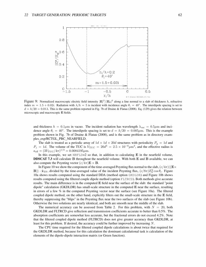
22 TARGET GENERATION: PERIODIC TARGETS 62

Figure 9: Normalized macroscopic electric field intensity |E|2/|E0|2 along a line normal to a slab of thickness h, refractiveindex m = 1.5 + 0.02i. Radiation with λ/h = 5 is incident with incidence angle θi = 40. The interdipole spacing is set tod = h/20 = 0.01λ. This is the same problem reported in Fig. 7b of Draine & Flatau (2008). Eq. (129) gives the relation betweenmicroscopic and macroscopic E fields.

and thickness h = 0.1µm in vacuo. The incident radiation has wavelength λvac = 0.5µm and inci-dence angle θi = 40. The interdipole spacing is set to d = h/20 = 0.005µm. This is the exampleproblem shown in Fig. 7b of Draine & Flatau (2008), and is the same problem as in directory exam-ples_exp/RCTGL_PBC_NEARFIELD.

The slab is treated as a periodic array of 1d × 1d × 20d structures with periodicity Py = 1d andPz = 1d. The volume of the TUC is VTUC = 20d3 = 2.5 × 10−6µm3, and the effective radius isaeff = (3VTUC/4π)1/3 = 0.0084195µm.

In this example, we set NRFLD=2 so that, in addition to calculating E in the nearfield volume,DDSCAT 7.3 will calculate B throughout the nearfield volume. With both E and B available, we canalso compute the Poynting vector (c/4π)E×B.

In Figure 10 we show the component of the time-averaged Poynting flux normal to the slab, (c/4π)〈(E×B)〉 · xTF, divided by the time-averaged value of the incident Poynting flux, (c/8π)E2

0 cos θi. Figure10a shows results computed using the standard DDA (method option GKDLDR) and Figure 10b showsresults computed using the filtered couple dipole method (option FLTRCD). Both methods give accurateresults. The main difference is in the computed E field near the surface of the slab: the standard "pointdipole" calculation (GKDLDR) has small-scale structure in the computed E near the surface, resultingin errors of a few % in the computed Poynting vector near the surface (see Figure 10a). The filteredcoupled dipole method, on the other hand, explicitly filters out the small-scale structure in the E field,thereby suppressing the "blips" in the Poynting flux near the two surfaces of the slab (see Figure 10b).Otherwise the two solutions are nearly identical, and both are smooth near the middle of the slab.

The numerical accuracy can be assessed from Table 2. For this problem, with N = 20, bothGKDLDR and FLTRCD give reflection and transmission coefficients accurate to better than 0.5%. Theabsorption coefficients are somewhat less accurate, but the fractional errors do not exceed 4.2%. Notethat the filtered coupled dipole method (FLTRCD) does not give greater accuracy than GKDLDR, atleast for this problem. If desired, the accuracy could be further improved by increasing N .

The CPU time required for the filtered coupled dipole calculations is about twice that required forthe GKDLDR method, because for this calculation the dominant calculational task is calculation of theelements of the dipole-dipole interaction matrix (or Green function).

22 TARGET GENERATION: PERIODIC TARGETS 63

Figure 10: Component of Poynting flux normal to a slab of thickness h = 0.10µm, refractive indexm = 1.5+0.02i. Radiationwith λ/h = 5 is incident with incidence angle θi = 40. The interdipole spacing is set to d = h/20 = 0.005µm. This is theproblem considered in Fig. 7b of Draine & Flatau (2008). Left: obtained with DDA method GKDLDR. Right: obtained with DDAmethod FLTRCD. The red and blue lines show (1−R) for xTF < −0.1µm, and T for xTF > 0, where R and T are the reflectionand transmission coefficients. The blue (dashed) lines correspond to the exact solution for T and R. The red (solid) line uses thevalues of T and R computed by DDSCAT 7.3: T‖ = S11(θT ) + S12(θT ), R‖ = S11(θR) + S12(θR), T⊥ = S11(θT )− S12(θT ),R⊥ = S11(θR)− S12(θR), with Sij from the output file w000r000k000.sca, θT = 40, and θR = 140.

22.10 RECRECPBC = Rectangular solid resting on top of another rectangularsolid, repeated periodically in target y and z directions using periodic boundaryconditionsThe TUC consists of a single rectangular “brick”, of material 1, resting on top of a second rectangularbrick, of material 2. The centroids of the two bricks along a line in the xTF direction. The bricks are as-sumed to be homogeneous, and materials 1 and 2 are assumed to be isotropic. The TUC is then repeatedin the yTF- and zTF-directions, with periodicities SHPAR4 × d and SHPAR5 × d. is the total volume ofsolid material in one TUC. This option requires 8 shape parameters:The pertinent line in ddscat.par should read

SHPAR1 SHPAR2 SHPAR3 SHPAR4 SHPAR5 SHPAR6 SHPAR7 SHPAR8

whereSHPAR1 = (upper brick thickness)/d in the xTF directionSHPAR2 = (upper brick thickness)/d in the yTF directionSHPAR3 = (upper brick thickness)/d in the zTF directionSHPAR4 = (lower brick thickness)/d in the xTF directionSHPAR5 = (lower brick thickness)/d in the yTF directionSHPAR6 = (lower brick thickness)/d in the zTF directionSHPAR7 = periodicity/d in the yTF directionSHPAR8 = periodicity/d in the zTF direction

22 TARGET GENERATION: PERIODIC TARGETS 64

Table 2: Results for m = 1.5 + 0.02i, h/λ = 0.2, θi = 40

quantity exact GKDLDR FLTRCDR‖ 0.051875 0.05179 0.051740R⊥ 0.25046 0.25047 0.25042T‖ 0.89545 0.89534 0.89592T⊥ 0.70280 0.70524 0.70478A‖ 0.052675 0.052482 0.052259A⊥ 0.046748 0.044970 0.044801

R‖ + T‖ +A‖ 1 0.99961 0.99992R⊥ + T⊥ +A⊥ 1 1.00068 1.00000

R‖/exact− 1 0 −0.0017 −0.0026R⊥/exact− 1 0 +0.0001 −0.0002T‖/exact− 1 0 −0.0001 +0.0005T⊥/exact− 1 0 +0.0035 +0.0042A‖/exact− 1 0 −0.0037 −0.0079A⊥/exact− 1 0 −0.0380 −0.0416

CPU time (s) (2.53GHz Intel, 1 core) – 1298. 2770.

The actual numbers of dipoles N1x, N1y , N1z , along each dimension of the upper brick, and N2x,N2y , N2z along each dimension of the lower brick, must be integers. Usually, N1x = nint(SHPAR1),N1y = nint(SHPAR2), N1z = nint(SHPAR3), N2x = nint(SHPAR4), N2y = nint(SHPAR5), N2z =nint(SHPAR6), where nint(x) is the integer nearest to x, but under some circumstances N1x, N1y , N1z ,N2x, N2y , N2z might be larger or smaller by 1 unit.

The overall size of the TUC (in terms of numbers of dipoles) is determined by parameters SHPAR1

– SHPAR6:N = (N1x ×N1y ×N1z) + (N2x ×N2y ×N2z) (38)

The physical size of the TUC is specified by the value of aeff (in physical units, e.g. cm), specified in thefile ddscat.par:

d = (4π/3N)1/3aeff (39)

The periodicity in the yTF and zTF directions is determined by parameters SHPAR7 and SHPAR8.The periodicity should not be smaller than the extent of the target, so that one should have

SHPAR7 ≥ max(SHPAR2, SHPAR5)SHPAR8 ≥ max(SHPAR3, SHPAR6)

The target is a periodic structure, of infinite extent in the yTF and zTF directions. The target axes areset to a1 = xTF – i.e., normal to the “slab” – and a2 = yTF. The orientation of the incident radiationrelative to the target is, as for all other targets, set by the usual orientation angles β, Θ, and Φ (see §19above) specifying the orientation of the target axes a1 and a2 relative to the direction of incidence; forexample, Θ = 0 would be for radiation incident normal to the slab.

The scattering directions are specified by specifying the diffraction order (M,N); for each diffrac-tion order one transmitted wave direction and one reflected wave direction will be calculated, with thedimensionless 4 × 4 scattering matrix S(2d) calculated for each scattering direction. At large distancesfrom the infinite slab, the scattered Stokes vector in the (M,N) diffraction order is

Isca,i(M,N) =

4∑j=1

S(2d)ij Iin,j (40)

where Iin,j is the incident Stokes vector. See Draine & Flatau (2008) for interpretation of the Sij astransmission and reflection efficiencies.

22 TARGET GENERATION: PERIODIC TARGETS 65

22.11 SLBHOLPBC = Target consisting of a periodic array of rectangular blocks,each containing a cylindrical holeIndividual blocks have extent (a, b, c) in the (xTF, yTF, zTF) directions, and the cylindrical hole hasradius r. The period in the yTF-direction is Py , and the period in the zTF-direction is Pz .The pertinent line in ddscat.par should consist ofSHPAR1 SHPAR2 SHPAR3 SHPAR4 SHPAR5 SHPAR6

where SHPAR1 = a/d (d is the interdipole spacing)SHPAR2 = b/aSHPAR3 = c/aSHPAR4 = r/aSHPAR5 = Py/dSHPAR6 = Pz/d.Ideally, a/d =SHPAR1, b/d =SHPAR2×SHPAR1, and c/d =SHPAR3×SHPAR1 will be integers (sothat the cubic lattice can accurately approximate the desired target). If Py = 0 and Pz > 0 the target isperiodic in the zTF-direction only.If Py > 0 and Pz = 0 the target is periodic in the yTF-direction only.If Py > 0 it is required that Py ≥ b, and if Pz > 0 it is required that Pz ≥ c, so that the blocks do notoverlap.With Py = b and Pz = c, the blocks are juxtaposed to form a periodic array of cylindrical holes in asolid slab.Example: ddscat_SLBHOLPBC.par is a sample ddscat.par for a periodic array of cylindricalholes in a slab of thickness a, with holes of radius r, and period Py and Pd

22.12 SPHRN_PBC = Target consisting of group of N spheres, extended in tar-get y and z directions using periodic boundary conditionsThis option causes DDSCAT to create a target consisting of a periodic array of N−sphere structures,where one N−sphere structure consists of N spheres, just as for target option NANSPH (see §21.23).Each sphere can be of arbitrary composition, and can be anisotropic if desired. Information for the de-scription of one N -sphere structure is supplied via an external file, just as for target option NANSPH –see §21.23).

Let us refer to a single N -sphere structure as the Target Unit Cell (TUC). The TUC is then repeatedin the yTF- and zTF-directions, with periodicities PYAEFF×aeff and PZAEFF×aeff , where aeff ≡(3VTUC/4π)1/3, where VTUC is the total volume of solid material in one TUC. This option requires3 shape parameters:DIAMX = maximum extent of target in the target frame x direction/dPYAEFF = periodicity in target y direction/aeff

PZAEFF = periodicity in target z direction/aeff .The pertinent line in ddscat.par should read

SHPAR1 SHPAR2 SHPAR3 ‘filename’ (quotes must be used)

whereSHPAR1 = target diameter in x direction (in Target Frame) in units of dSHPAR2= PYAEFFSHPAR3= PZAEFF.filename is the name of the file specifying the locations and relative sizes of the spheres.

The overall size of the TUC (in terms of numbers of dipoles) is determined by parameter SHPAR1,which is the extent of the multisphere target in the x-direction, in units of the lattice spacing d. Thephysical size of the TUC is specified by the value of aeff (in physical units, e.g. cm), specified in the fileddscat.par.

22 TARGET GENERATION: PERIODIC TARGETS 66

The location of the spheres in the TUC, and their composition, is specified in file ‘filename’. Pleaseconsult §21.23 above for detailed information concerning the information in this file, and its arrangement.

Note that while the spheres can be anisotropic and of differing composition, they can of course alsobe isotropic and of a single composition, in which case the relevant lines in the file ’filename’ shouldreadx1 y1 z1 r1 1 1 1 0 0 0x2 y2 z2 r2 1 1 1 0 0 0x3 y3 z3 r3 1 1 1 0 0 0...i.e., every sphere has isotropic composition ICOMP=1 and the three dielectric function orientation anglesare set to zero.

When the user uses target option SPHRN_PBC, the target now becomes a periodic structure, ofinfinite extent in the target y- and z- directions. The target axis a1 = xLF = (1, 0, 0)TF – i.e., normalto the “slab” – and target axis a2 = yLF = (0, 1, 0)TF. The orientation of the incident radiation relativeto the target is, as for all other targets, set by the usual orientation angles β, Θ, and Φ (see §19 above).The scattering directions are, just as for other targets, determined by the scattering angles θs, φs (see §23below).

The scattering problem for this infinite structure, assumed to be illuminated by an incident monochro-matic plane wave, is essentially solved “exactly”, in the sense that the electric polarization of each of theconstituent dipoles is due to the electric field produced by the incident plane wave plus all of the otherdipoles in the infinite target.

However, the assumed target will, of course, act as a perfect diffraction grating if the scattered radia-tion is calculated as the coherent sum of all the oscillating dipoles in this periodic structure: the far-fieldscattered intensity would be zero in all directions except those where the Bragg scattering condition issatisfied, and in those directions the far-field scattering intensity would be infinite.

To suppress this singular behavior, we calculate the far-field scattered intensity as though the sepa-rate TUCs scatter incoherently. The scattering efficiency Qsca and the absorption efficiency Qabs aredefined to be the scattering and absorption cross section per TUC, divided by πa2

eff , where aeff ≡(3VTUC/4π)1/3, where VTUC is the volume of solid material per TUC.

Note: the user is allowed to set the target periodicity in the target yTF (or zTF) direction to values thatcould be smaller than the total extent of one TUC in the target yTF (or zTF) direction. This is physicallyallowable, provided that the spheres from one TUC do not overlap with the spheres from neighboringTUCs. Note that DDSCAT does not check for such overlap.

22.12.1 Sample calculation in directory examples_exp/SPHRN_PBC

Subdirectory examples_exp/SPHRN_PBC contains ddscat.par to calculate scattering by a doubly-periodic array with the target unit cell consisting of a random cluster of 16 spheres. The calculation iscarried out with double precision arithmetic. Because convergence is slow, the error tolerance is setto TOL = 5.e-5 rather than the usual 1.e-5, and the maximum number of iterations allowed isincreased to MXITER = 2000.

22.13 TRILYRPBC = Three stacked rectangular blocks, repeated periodicallyThe target unit cell (TUC) consists of a stack of 3 rectangular blocks with centers on the xTF axis. TheTUC is repeated in either the yTF direction, the zTF direction, or both. A total of 11 shape parametersmust be specified:SHPAR1 = x-thickness of upper layer/d [material 1]SHPAR2 = y-width/d of upper layerSHPAR3 = z-width/d of upper layerSHPAR4 = x-thickness/d of middle layer [material 2]SHPAR5 = y-width/d of middle layerSHPAR6 = z-width/d of middle layerSHPAR7 = x-width/d of lower layer

23 SCATTERING DIRECTIONS 67

SHPAR8 = y-width/d of lower layerSHPAR9 = z-width/d of lower layerSHPAR10 = period/d in y directionSHPAR11= period/d in z direction

23 Scattering Directions

23.1 Isolated Finite TargetsDDSCAT calculates scattering in selected directions, and elements of the scattering matrix are reportedin the output files wxxxryyykzzz.sca . The scattering direction is specified through angles θs and φs(not to be confused with the angles Θ and Φ which specify the orientation of the target relative to theincident radiation!).

For isolated finite targets (i.e., PBC not employed) there are two options for specifying the scatter-ing direction, with the option determined by the value of the string CMDFRM read from the input fileddscat.par.

1. If the user specifies CMDFRM=’LFRAME’, then the angles θ, φ input from ddscat.par areunderstood to specify the scattering directions relative to the Lab Frame (the frame where theincident beam is in the x−direction).When CMDFRM=’LFRAME’, the angle θ is simply the scattering angle θs: the angle between theincident beam (in direction xLF) and the scattered beam (θs = 0 for forward scattering, θs = 180

for backscattering).The angle φ specifies the orientation of the “scattering plane” relative to the xLF − yLF plane.When φ = 0 the scattering plane is assumed to coincide with the xLF− yLF plane. When φ = 90

the scattering plane is assumed to coincide with the xLF − zLF plane. Within the scattering planethe scattering directions are specified by 0 ≤ θ ≤ 180. Thus:

ns = xLF cos θ + yLF sin θ cosφ+ zLF sin θ sinφ , (41)

2. If the user specifies CMDFRM=’TFRAME’, then the angles θ, φ input from ddscat.par areunderstood to specify the scattering directions ns relative to the Target Frame (the frame definedby target axes xTF, yTF, zTF). θ is the angle between ns and xTF, and φ is the angle between thens − xTF plane and the xTF − yTF plane. Thus:

ns = xTF cos θ + yTF sin θ cosφ+ zTF sin θ sinφ . (42)

Scattering directions for which the scattering properties are to be calculated are set in the parameterfile ddscat.par by specifying one or more scattering planes (determined by the value of φs) and foreach scattering plane, the number and range of θs values. The only limitation is that the number ofscattering directions not exceed the parameter MXSCA in DDSCAT.f (in the code as distributed it is setto MXSCA=1000).

23.2 Scattering Directions for Targets that are Periodic in 1 DimensionFor targets that are periodic, scattering is only allowed in certain directions (Draine & Flatau 2008, see).If the user has chosen a PBC target (e.g, CYLNDRPBC, HEXGONPBC, or RCTGL_PBC), SPHRN_PBCbut has set one of the periodicities to zero, then the target is periodic in only one dimension – e.g.,CYLNDRPBC could be used to construct a single infinite cylinder.

In this case, the scattering directions are specified by giving an integral diffraction order M =0,±1,±2, ... and one angle, the azimuthal angle ζ around the target repetition axis. The diffractionorder M determines the projection of ks onto the repetition direction. For a given order M , the scatter-ing angles with ζ = 0→ 2π form a cone around the repetition direction.

23 SCATTERING DIRECTIONS 68

For example, if PYD > 0 (target repeating in the yTF direction), then M determines the value ofksy = ks · yTF, where yTF is the unit vector in the Target Frame y−direction:

ksy = k0y + 2πM/Ly (43)

where k0y ≡ k0 · yTF, where k0 is the incident k vector. Note that the diffraction order M must satisfythe condition

(k0y − k0)(Ly/2π) < M < (k0 − k0y)(Ly/2π) (44)

where Ly = PYD×d is the periodicity along the y axis in the Target Frame. M = 0 is always an alloweddiffraction order.

The azimuthal angle ζ defines a right-handed rotation of the scattering direction around the targetrepetition axis. Thus for a target repetition axis yTF,

ksx = k⊥ cos ζ , (45)ksz = k⊥ sin ζ , (46)

where k⊥ = (k20 − k2

sy)1/2, with ksy = k0y + 2πM/Ly . For a target with repetition axis zTF,

ksx = k⊥ cos ζ , (47)ksy = k⊥ sin ζ , (48)

where k⊥ = (k20 − k2

sz)1/2, ksz = k0z + 2πM/Lz .

The user selects a diffraction order M and the azimuthal angles ζ to be used for that M via one linein ddscat.par. An example would be to use CYLNDRPBC to construct an infinite cylinder with thecylinder direction in the yTF direction: e.g., examples_exp/CYLNDRPBC/ddscat.par :

’ ========== Parameter file for v7.3 ===================’’**** Preliminaries ****’’NOTORQ’ = CMTORQ*6 (DOTORQ, NOTORQ) -- either do or skip torque calculations’PBCGS2’ = CMDSOL*6 (PBCGS2, PBCGST, GPBICG, QMRCCG, PETRKP) -- CCG method’GPFAFT’ = CMETHD*6 (GPFAFT, FFTMKL) -- FFT method’GKDLDR’ = CALPHA*6 (GKDLDR, LATTDR, FLTRCD) -- DDA method’NOTBIN’ = CBINFLAG (NOTBIN, ORIGIN, ALLBIN)’**** Initial Memory Allocation ****’100 100 100 = dimensioning allowance for target generation’**** Target Geometry and Composition ****’’CYLNDRPBC’ = CSHAPE*9 shape directive1 64.499 2 1.0 0.0 = shape parameters 1 - 71 = NCOMP = number of dielectric materials’../diel/m1.33_0.01’ = file with refractive index 1’**** Additional Nearfield calculation? ****’0 = NRFLD (=0 to skip nearfield calc., =1 to calculate nearfield E)0.0 0.0 0.0 0.0 0.0 0.0 (fract. extens. of calc. vol. in -x,+x,-y,+y,-z,+z)’**** Error Tolerance ****’1.00e-5 = TOL = MAX ALLOWED (NORM OF |G>=AC|E>-ACA|X>)/(NORM OF AC|E>)’**** Maximum number of iterations ****’200 = MXITER’**** Integration limiter for PBC calculations ****’1.00e-3 = GAMMA (1e-2 is normal, 3e-3 for greater accuracy)’**** Angular resolution for calculation of <cos>, etc. ****’0.5 = ETASCA (number of angles is proportional to [(3+x)/ETASCA]^2 )’**** Vacuum wavelengths (micron) ****’6.283185 6.283185 1 ’LIN’ = wavelengths (first,last,how many,how=LIN,INV,LOG)’**** Refractive index of ambient medium’1.0000 = NAMBIENT’**** Effective Radii (micron) **** ’2.8555 2.8555 1 ’LIN’ = aeff (first,last,how many,how=LIN,INV,LOG)’**** Define Incident Polarizations ****’(0,0) (1.,0.) (0.,0.) = Polarization state e01 (k along x axis)2 = IORTH (=1 to do only pol. state e01; =2 to also do orth. pol. state)’**** Specify which output files to write ****’1 = IWRKSC (=0 to suppress, =1 to write ".sca" file for each target orient.’**** Specify Target Rotations ****’

23 SCATTERING DIRECTIONS 69

0. 0. 1 = BETAMI, BETAMX, NBETA (beta=rotation around a1)60. 60. 1 = THETMI, THETMX, NTHETA (theta=angle between a1 and k)0. 0. 1 = PHIMIN, PHIMAX, NPHI (phi=rotation angle of a1 around k)’**** Specify first IWAV, IRAD, IORI (normally 0 0 0) ****’0 0 0 = first IWAV, first IRAD, first IORI (0 0 0 to begin fresh)’**** Select Elements of S_ij Matrix to Print ****’6 = NSMELTS = number of elements of S_ij to print (not more than 9)11 12 21 22 31 41 = indices ij of elements to print’**** Specify Scattered Directions ****’’TFRAME’ = CMDFRM (LFRAME, TFRAME for Lab Frame or Target Frame)1 = NPLANES = number of scattering cones0. 0. 180. 1 = OrderM zetamin zetamax dzeta for scattering cone 1

In this example, a single diffraction order M = 0 is selected, and ζ is to run from ζmin = 0 toζmax = 180 in increments of δζ = 0.05.

There may be additional lines, one per diffraction order. Remember, however, that every diffractionorder must satisfy eq. (44).

23.3 Scattering Directions for Targets for Doubly-Periodic TargetsIf the user has specified nonzero periodicity in both the y and z directions, then the scattering direc-tions are specified by two integers – the diffraction orders M,N for the y, z directions. The scatteringdirections are

ks = ± knk0

(k0 · xTF) xTF +

(k0 · yTF +

2πM

Ly

)yTF +

(k0 · zTF +

2πN

Lz

)zTF (49)

kn ≡

[k2

0 −(

k0 · yTF +2πM

Ly

)2

+

(k0 · zTF +

2πN

Lz

)2]1/2

(50)

where the + sign gives transmission, and the − sign gives reflection. The integers M and N musttogether satisfy the inequality

(k0 · yTF + 2πM/Ly)2 + (k0 · zTF + 2πN/Lz)2 < k2

0 (51)

which, for small values of Ly and Lz , may limit the scattering to only (M,N) = (0, 0). [Of course,(0, 0) is always allowed]. For each (M,N) specified in ddscat.par, DDSCAT 7.3 will calculatethe generalized Mueller matrix S(2d)

ij (M,N) – see §27.2. At large distances from the infinite slab, thescattered Stokes vector in the (M,N) diffraction order is

Isca,i(M,N) =

4∑j=1

S(2d)ij (M,N)Iin,j (52)

where Iin,j is the incident Stokes vector, and S(2d)ij (M,N) is the generalization of the 4 × 4 Müller

scattering matrix to targets that are periodic in 2-directions (Draine & Flatau 2008). There are distinctS

(2d)ij (M,N) for transmission and for reflection, corresponding to the ± in eq. (49).

Draine & Flatau (2008) (eq. 69-71) show how the S(2d)ij (M,N) are easily related to familiar "trans-

mission coefficients" and "reflection coefficients".Here is examples_exp/RCTGL_PBC/ddscat.par file as an example:

’ =========== Parameter file for v7.3 ===================’’**** Preliminaries ****’’NOTORQ’ = CMTORQ*6 (DOTORQ, NOTORQ) -- either do or skip torque calculations’PBCGS2’ = CMDSOL*6 (PBCGS2,PBCGST, GPBICG, QMRCCG, PETRKP) -- CCG method’GPFAFT’ = CMDFFT*6 (GPFAFT, FFTMKL) -- FFT method’GKDLDR’ = CALPHA*6 (GKDLDR, LATTDR, FLTRCD) -- DDA method’NOTBIN’ = CBINFLAG (NOTBIN, ORIBIN, ALLBIN)’**** Initial Memory Allocation ****’100 100 100 = dimensioning allowance for target generation

24 INCIDENT POLARIZATION STATE 70

’**** Target Geometry and Composition ****’’RCTGL_PBC’ = CSHAPE*9 shape directive20 1 1 1 1 = shpar1 - shpar5 (see README.txt)1 = NCOMP = number of dielectric materials’../diel/m1.50_0.02’ = refractive index 1’**** Additional Nearfield calculation? ****’0 = NRFLD (=0 to skip nearfield calc., =1 to calculate nearfield E)0.0 0.0 0.0 0.0 0.0 0.0 (fract. extens. of calc. vol. in -x,+x,-y,+y,-z,+z)’**** Error Tolerance ****’1.00e-5 = TOL = MAX ALLOWED (NORM OF |G>=AC|E>-ACA|X>)/(NORM OF AC|E>)’**** Maximum number of iterations ****’100 = MXITER’**** Integration limiter for PBC calculations ****’1.00e-2 = GAMMA (1e-2 is normal, 3e-3 for greater accuracy)’**** Angular resolution for calculation of <cos>, etc. ****’1. = ETASCA (number of angles is proportional to [(3+x)/ETASCA]^2 )’**** Vacuum wavelengths (micron) ****’0.5 0.5 1 ’LIN’ = wavelengths (first,last,how many,how=LIN,INV,LOG)’**** Refractive index of ambient medium’1.000 = NAMBIENT’**** Effective Radii (micron) **** ’0.0084195 0.0084195 1 ’LIN’ = aeff (first,last,how many,how=LIN,INV,LOG)’**** Define Incident Polarizations ****’(0,0) (1.,0.) (0.,0.) = Polarization state e01 (k along x axis)2 = IORTH (=1 to do only pol. state e01; =2 to also do orth. pol. state)’**** Specify which output files to write ****’1 = IWRKSC (=0 to suppress, =1 to write ".sca" file for each target orient.’**** Prescribe Target Rotations ****’0. 0. 1 = BETAMI, BETAMX, NBETA (beta=rotation around a1)40. 40. 1 = THETMI, THETMX, NTHETA (theta=angle between a1 and k)0. 0. 1 = PHIMIN, PHIMAX, NPHI (phi=rotation angle of a1 around k)’**** Specify first IWAV, IRAD, IORI (normally 0 0 0) ****’0 0 0 = first IWAV, first IRAD, first IORI (0 0 0 to begin fresh)’**** Select Elements of S_ij Matrix to Print ****’6 = NSMELTS = number of elements of S_ij to print (not more than 9)11 12 21 22 31 41 = indices ij of elements to print’**** Specify Scattered Directions ****’’TFRAME’ = CMDFRM (LFRAME, TFRAME for Lab Frame or Target Frame)1 = NORDERS = number of diffraction orders for transmission0. 0.

24 Incident Polarization StateRecall that the “Lab Frame” is defined such that the incident radiation is propagating along the xLF

axis. DDSCAT allows the user to specify a general elliptical polarization for the incident radiation, byspecifying the (complex) polarization vector e01. The orthonormal polarization state e02 = xLF × e∗01

is generated automatically if ddscat.par specifies IORTH=2.For incident linear polarization, one can simply set e01 = y by specifying

(0,0) (1,0) (0,0)in ddscat.par; then e02 = z. For polarization mode e01 to correspond to right-handed circular po-larization, set e01 = (y + iz)/

√2 by specifying (0,0) (1,0) (0,1) in ddscat.par (DDSCAT

automatically takes care of the normalization of e01); then e02 = (iy + z)/√

2, corresponding to left-handed circular polarization.

25 Averaging over Scattering Directions: g(1) = 〈cos θs〉, etc.

25.1 Angular AveragingAn example of scattering by a nonspherical target is shown in Fig. 11, showing the scattering for a tiltedcube. Results are shown for four different scattering planes.

DDSCAT automatically carries out numerical integration of various scattering properties, including

25 AVERAGING OVER SCATTERING DIRECTIONS: G(1) = 〈COS θS〉, ETC. 71

Figure 11: Scattered intensity for incident unpolarized light for a cube with m = 1.5 + 0.001i and x = 2πaeff/λ = 6.5 (i.e.,d/λ = 1.6676, where d is the length of a side). The cube is tilted with respect to the incident radiation, with Θ = 30, and rotatedby β = 15 around its axis to break reflection symmetry. The Mueller matrix element S11 is shown for 4 different scattering planes.The strong forward scattering lobe is evident. It is also seen that the scattered intensity is a strong function of scattering angle φs aswell as θs – at a given value of θs (e.g., θs = 120), the scattered intensity can vary by orders of magnitude as φs changes by 90.

• 〈cos θs〉;• 〈cos2 θs〉;• g = 〈cos θs〉xLF + 〈sin θs cosφs〉y + 〈sin θs sinφs〉z (see §16);

• QΓ, provided option DOTORQ is specified (see §16).

The angular averages are accomplished by evaluating the scattered intensity for selected scattering di-rections (θs, φs), and taking the appropriately weighted sum. Suppose that we have Nθ different valuesof θs,

θ = θj , j = 1, ..., Nθ , (53)

and for each value of θj , Nφ(j) different values of φs:

φs = φj,k, k = 1, ..., Nφ(j) . (54)

For a given j, the values of φj,k are assumed to be uniformly spaced: φj,k+1 − φj,k = 2π/Nφ(j). Theangular average of a quantity f(θs, φs) is approximated by

〈f〉 ≡ 1

4π

∫ π

0

sin θsdθs

∫ 2π

0

dφsf(θs, φs) ≈1

4π

Nθ∑j=1

Nφ(j)∑k=1

f(θj , φj,k)Ωj,k (55)

Ωj,k =π

Nφ(j)[cos(θj−1)− cos(θj+1)] , j = 2, ..., Nθ − 1 . (56)

Ω1,k =2π

Nφ(1)

[1− cos(θ1) + cos(θ2)

2

], (57)

ΩNθ,k =2π

Nφ(Nθ)

[cos(θNθ−1) + cos(θNθ

)

2+ 1

]. (58)

25 AVERAGING OVER SCATTERING DIRECTIONS: G(1) = 〈COS θS〉, ETC. 72

For a sufficiently large number of scattering directions

Nsca ≡Nθ∑j=1

Nφ(j) (59)

the sum (55) approaches the desired integral, but the calculations can be a significant cpu-time burden,so efficiency is an important consideration.

25.2 Selection of Scattering Angles θs, φs

Beginning with DDSCAT 6.1, an improved approach is taken to evaluation of the angular average. Sincetargets with large values of x = 2πaeff/λ in general have strong forward scattering, it is important toobtain good sampling of the forward scattering direction. To implement a preferential sampling of theforward scattering directions, the scattering directions (θ, φ) are chosen so that θ values correspondto equal intervals in a monotonically increasing function s(θ). The function s(θ) is chosen to have anegative second derivative d2s/dθ2 < 0 so that the density of scattering directions will be higher forsmall values of θ. DDSCAT takes

s(θ) = θ +θ

θ + θ0. (60)

This provides increased resolution (i.e., increased ds/dθ) for θ < θ0. We want this for the forwardscattering lobe, so we take

θ0 =2π

1 + x. (61)

The θ values run from θ = 0 to θ = π, corresponding to uniform increments

∆s =1

Nθ − 1

(π +

π

π + θ0

). (62)

If we now require that

max[∆θ] ≈ ∆s

(ds/dθ)θ=π= η

π/2

3 + x, (63)

we determine the number of values of θ:

Nθ = 1 +2(3 + x)

η

[1 + 1/(π + θ0)]

[1 + θ0/(π + θ0)2]. (64)

Thus for small values of x, max[∆θ] = 30η, and for x 1, max[∆θ] → 90η/x. For a sphere,minima in the scattering pattern are separated by ∼ 180/x, so η = 1 would be expected to marginallyresolve structure in the scattering function. Smaller values of η will obviously lead to improved samplingof the scattering function, and more accurate angular averages.

The scattering angles θj used for the angular averaging are then given by

θj =(sj − 1− θ0) +

[(1 + θ0 − sj)2 + 4θ0sj

]1/22

, (65)

where

sj =(j − 1)π

Nθ − 1

[1 +

1

π + θ0

]j = 1, ..., Nθ . (66)

For each θj , we must choose values of φ. For θ1 = 0 and θNθ= π only a single value of φ is needed

(the scattering is independent of φ in these two directions). For 0 < θj < π we use

Nφ = max 3,nint [4π sin(θj)/(θj+1 − θj−1)] , (67)

where nint = nearest integer. This provides sampling in φ consistent with the sampling in θ.

25 AVERAGING OVER SCATTERING DIRECTIONS: G(1) = 〈COS θS〉, ETC. 73

Figure 12: Errors in 〈cos θ〉 and 〈cos2 θ〉 calculated for aN = 17904 dipole pseudosphere withm = 1.33+0.01i, as functionsof x = 2πa/λ. Results are shown for different values of the parameter η.

Figure 13: Same as Fig. 12, but for a N = 32768 dipole cube with m = 1.5 + 0.001i.

25.3 Accuracy of Angular Averaging as a Function of ηFigure 12 shows the absolute errors in 〈cos θ〉 and 〈cos2 θ〉 calculated for a sphere with refractive indexm = 1.33 + 0.01i using the above prescription for choosing scattering angles. The error is shown as afunction of scattering parameter x. We see that accuracies of order 0.01 are attained with η = 1, and thatthe above prescription provides an accuracy which is approximately independent of x. We recommendusing values of η ≤ 1 unless accuracy in the angular averages is not important.

26 SCATTERING BY FINITE TARGETS: THE MUELLER MATRIX 74

26 Scattering by Finite Targets: The Mueller Matrix

26.1 Two Orthogonal Incident Polarizations (IORTH=2)Subsection 26.1 is intended for those studying the internals of DDSCAT to see how it obtains the ele-ments of the scattering amplitude matrix (see Bohren & Huffman 1983)(

S2 S3

S4 S1

). (68)

Unless you are interested in such computational details, you can skip this subsection and go forward to§26.2.

Throughout the following discussion, xLF, yLF, zLF are unit vectors defining the Lab Frame (thusk0 = xLF).

DDSCAT internally computes the scattering properties of the dipole array in terms of a complexscattering matrix fml(θs, φs) (Draine 1988), where index l = 1, 2 denotes the incident polarization state,m = 1, 2 denotes the scattered polarization state, and θs,φs specify the scattering direction. NormallyDDSCAT is used with IORTH=2 in ddscat.par, so that the scattering problem will be solved forboth incident polarization states (l = 1 and 2); in this subsection it will be assumed that this is the case.

Incident polarization states l = 1, 2 correspond to polarization states e01, e02; recall that polarizationstate e01 is user-specified, and e02 = k0 × e∗01 = xLF × e∗01.14,15 In the DDSCAT code, which followsthe convention in Draine (1988), scattered polarization state m = 1 corresponds to linear polarizationof the scattered wave parallel to the scattering plane (e1 = e‖s = θs) and m = 2 corresponds to linearpolarization perpendicular to the scattering plane (in the +φs direction: e2 = φs). The scattering matrixfml was defined (Draine 1988) so that the scattered electric field Es is related to the incident electricfield Ei(0) at the origin (where the target is assumed to be located) by(

Es · θsEs · φs

)=

exp(iks · r)

kr

(f11 f12

f21 f22

)(Ei(0) · e∗01

Ei(0) · e∗02

). (69)

The 2×2 complex scattering amplitude matrix (with elements S1, S2, S3, and S4) is defined so that (seeBohren & Huffman 1983)(

Es · θs−Es · φs

)=

exp(iks · r)

−ikr

(S2 S3

S4 S1

)(Ei(0) · ei‖Ei(0) · ei⊥

), (70)

where ei‖, ei⊥ are (real) unit vectors for incident polarization parallel and perpendicular to the scatteringplane (with the customary definition of ei⊥ = ei‖ × k0 = ei‖ × xLF).

From (69,70) we may write(S2 S3

S4 S1

)(Ei(0) · ei‖Ei(0) · ei⊥

)= −i

(f11 f12

−f21 −f22

)(Ei(0) · e∗01

Ei(0) · e∗02

). (71)

Let

a ≡ e∗01 · yLF , (72)b ≡ e∗01 · zLF , (73)c ≡ e∗02 · yLF , (74)d ≡ e∗02 · zLF . (75)

Note that since e01, e02 could be complex (i.e., elliptical polarization), the quantities a, b, c, d are com-plex. Then (

e∗01

e∗02

)=

(a bc d

)(yLF

zLF

)(76)

14 Draine (1988) adopted the convention e02 = x× e∗01. The customary definition of ei⊥ is ei⊥ ≡ ei‖× k0 (Bohren & Huffman1983). Thus, if e01 = ei‖, then e02 = −ei⊥.

15 A frequent choice is e01 = yLF, with e02 = xLF × yLF = zLF.

26 SCATTERING BY FINITE TARGETS: THE MUELLER MATRIX 75

and eq. (71) can be written(S2 S3

S4 S1

)(Ei(0) · ei‖Ei(0) · ei⊥

)= i

(−f11 −f12

f21 f22

)(a bc d

)(Ei(0) · yLF

Ei(0) · zLF

). (77)

The incident polarization states ei‖ and ei⊥ are related to yLF, zLF by(ei‖ei⊥

)=

(cosφs sinφssinφs − cosφs

)(yLF

zLF

)(78)

(yLF

zLF

)=

(cosφs sinφssinφs − cosφs

)(ei‖ei⊥

). (79)

The angle φs specifies the scattering plane, with

cosφs = φs · zLF = e2 · zLF , (80)sinφs = −φs · yLF = −e2 · yLF . (81)

Substituting (79) into (77) we obtain(S2 S3

S4 S1

)(Ei(0) · ei‖Ei(0) · ei⊥

)= i

(−f11 −f12

f21 f22

)(a bc d

)(cosφs sinφssinφs − cosφs

)(Ei(0) · ei‖Ei(0) · ei⊥

)(82)

Eq. (82) must be true for all Ei(0); hence we obtain an expression for the complex scatteringamplitude matrix in terms of the fml:(

S2 S3

S4 S1

)= i

(−f11 −f12

f21 f22

)(a bc d

)(cosφs sinφssinφs − cosφs

). (83)

This provides the 4 equations used in subroutine GETMUELLER to compute the scattering amplitudematrix elements:

S1 = −i [f21(b cosφs − a sinφs) + f22(d cosφs − c sinφs)] , (84)S2 = −i [f11(a cosφs + b sinφs) + f12(c cosφs + d sinφs)] , (85)S3 = i [f11(b cosφs − a sinφs) + f12(d cosφs − c sinφs)] , (86)S4 = i [f21(a cosφs + b sinφs) + f22(c cosφs + d sinφs)] . (87)

26.2 Stokes ParametersIt is both convenient and customary to characterize both incident and scattered radiation by 4 “Stokesparameters” – the elements of the “Stokes vector”. There are different conventions in the literature; weadhere to the definitions of the Stokes vector (I ,Q,U ,V ) adopted in the excellent treatise by Bohren &Huffman (1983), to which the reader is referred for further detail. Here are some examples of Stokesvectors (I,Q, U, V ) = (1, Q/I, U/I, V/I)I:

• (1, 0, 0, 0)I : unpolarized light (with intensity I);

• (1, 1, 0, 0)I : 100% linearly polarized with E parallel to the scattering plane;

• (1,−1, 0, 0)I : 100% linearly polarized with E perpendicular to the scattering plane;

• (1, 0, 1, 0)I : 100% linearly polarized with E at +45 relative to the scattering plane;

• (1, 0,−1, 0)I : 100% linearly polarized with E at -45 relative to the scattering plane;

• (1, 0, 0, 1)I : 100% right circular polarization (i.e., negative helicity);

• (1, 0, 0,−1)I : 100% left circular polarization (i.e., positive helicity).

26 SCATTERING BY FINITE TARGETS: THE MUELLER MATRIX 76

26.3 Relation Between Stokes Parameters of Incident and Scattered Radiation:The Mueller MatrixIt is convenient to describe the scattering properties of a finite target in terms of the 4 × 4 Mueller ma-trix Sij relating the Stokes parameters (Ii, Qi, Ui, Vi) and (Is, Qs, Us, Vs) of the incident and scatteredradiation:

IsQsUsVs

=1

k2r2

S11 S12 S13 S14

S21 S22 S23 S24

S31 S32 S33 S34

S41 S42 S43 S44

IiQiUiVi

. (88)

Once the amplitude scattering matrix elements are obtained, the Mueller matrix elements can be com-puted (Bohren & Huffman 1983):

S11 =(|S1|2 + |S2|2 + |S3|2 + |S4|2

)/2 ,

S12 =(|S2|2 − |S1|2 + |S4|2 − |S3|2

)/2 ,

S13 = Re (S2S∗3 + S1S

∗4 ) ,

S14 = Im (S2S∗3 − S1S

∗4 ) ,

S21 =(|S2|2 − |S1|2 + |S3|2 − |S4|2

)/2 ,

S22 =(|S1|2 + |S2|2 − |S3|2 − |S4|2

)/2 ,

S23 = Re (S2S∗3 − S1S

∗4 ) ,

S24 = Im (S2S∗3 + S1S

∗4 ) ,

S31 = Re (S2S∗4 + S1S

∗3 ) ,

S32 = Re (S2S∗4 − S1S

∗3 ) ,

S33 = Re (S1S∗2 + S3S

∗4 ) ,

S34 = Im (S2S∗1 + S4S

∗3 ) ,

S41 = Im (S4S∗2 + S1S

∗3 ) ,

S42 = Im (S4S∗2 − S1S

∗3 ) ,

S43 = Im (S1S∗2 − S3S

∗4 ) ,

S44 = Re (S1S∗2 − S3S

∗4 ) . (89)

These matrix elements are computed in DDSCAT and passed to subroutine WRITESCA which handlesoutput of scattering properties. Although the Muller matrix has 16 elements, only 9 are independent.

The user can select up to 9 distinct Muller matrix elements to be printed out in the output fileswxxxryyykzzz.sca and wxxxryyyori.avg; this choice is made by providing a list of indices in ddscat.par(see Appendix A).

If the user does not provide a list of elements, WRITESCA will provide a “default” set of 6 selectedelements: S11, S21, S31, S41 (these 4 elements describe the intensity and polarization state for scatteringof unpolarized incident radiation), S12, and S13.

In addition, WRITESCA writes out the linear polarization P of the scattered light for incident unpo-larized light (see Bohren & Huffman 1983):

P =(S2

21 + S231)1/2

S11. (90)

26.4 Polarization Properties of the Scattered RadiationThe scattered radiation is fully characterized by its Stokes vector (Is, Qs, Us, Vs). As discussed inBohren & Huffman (1983) (eq. 2.87), one can determine the linear polarization of the Stokes vector

26 SCATTERING BY FINITE TARGETS: THE MUELLER MATRIX 77

by operating on it by the Mueller matrix of an ideal linear polarizer:

Spol =1

2

1 cos 2ξ sin 2ξ 0

cos 2ξ cos2 2ξ cos 2ξ sin 2ξ 0sin 2ξ sin 2ξ cos 2ξ sin2 2ξ 0

0 0 0 0

(91)

where ξ is the angle between the unit vector θs parallel to the scattering plane (“SP”) and the “transmis-sion” axis of the linear polarizer. Therefore the intensity of light polarized parallel to the scattering planeis obtained by taking ξ = 0 and operating on (Is, Qs, Us, Vs) to obtain

I(Es ‖ SP) =1

2(Is +Qs) (92)

=1

2k2r2[(S11 + S21)Ii + (S12 + S22)Qi + (S13 + S23)Ui + (S14 + S24)Vi] . (93)

Similarly, the intensity of light polarized perpendicular to the scattering plane is obtained by takingξ = π/2:

I(Es ⊥ SP) =1

2(Is −Qs) (94)

=1

2k2r2[(S11 − S21)Ii + (S12 − S22)Qi + (S13 − S23)Ui + (S14 − S24)Vi] . (95)

26.5 Relation Between Mueller Matrix and Scattering Cross SectionsDifferential scattering cross sections can be obtained directly from the Mueller matrix elements by notingthat

Is =1

r2

(dCsca

dΩ

)s,i

Ii . (96)

Let SP be the “scattering plane”: the plane containing the incident and scattered directions of propaga-tion. Here we consider some special cases:

• Incident light unpolarized: Stokes vector si = I(1, 0, 0, 0):

– cross section for scattering with polarization Es ‖ SP:

dCsca

dΩ=

1

2k2

(|S2|2 + |S3|2

)=

1

2k2(S11 + S21) (97)

– cross section for scattering with polarization Es ⊥ SP:

dCsca

dΩ=

1

2k2

(|S1|2 + |S4|2

)=

1

2k2(S11 − S21) (98)

– total intensity of scattered light:

dCsca

dΩ=

1

2k2

(|S1|2 + |S2|2 + |S3|2 + |S4|2

)=

1

k2S11 (99)

• Incident light polarized with Ei ‖ SP: Stokes vector si = I(1, 1, 0, 0):

– cross section for scattering with polarization Es ‖ to SP:

dCsca

dΩ=

1

k2|S2|2 =

1

2k2(S11 + S12 + S21 + S22) (100)

– cross section for scattering with polarization Es ⊥ to SP:

dCsca

dΩ=

1

k2|S4|2 =

1

2k2(S11 + S12 − S21 − S22) (101)

26 SCATTERING BY FINITE TARGETS: THE MUELLER MATRIX 78

– total scattering cross section:

dCsca

dΩ=

1

k2

(|S2|2 + |S4|2

)=

1

k2(S11 + S12) (102)

• Incident light polarized with Ei ⊥ SP: Stokes vector si = I(1,−1, 0, 0):

– cross section for scattering with polarization Es ‖ to SP:

dCsca

dΩ=

1

k2|S3|2 =

1

2k2(S11 − S12 + S21 − S22) (103)

– cross section for scattering with polarization Es ⊥ SP:

dCsca

dΩ=

1

k2|S1|2 =

1

2k2(S11 − S12 − S21 + S22) (104)

– total scattering cross section:

dCsca

dΩ=

1

k2

(|S1|2 + |S3|2

)=

1

k2(S11 − S12) (105)

• Incident light linearly polarized at angle γ to SP: Stokes vector si = I(1, cos 2γ, sin 2γ, 0):

– cross section for scattering with polarization Es ‖ to SP:

dCsca

dΩ=

1

2k2[(S11 + S21) + (S12 + S22) cos 2γ + (S13 + S23) sin 2γ] (106)

– cross section for scattering with polarization Es ⊥ SP:

dCsca

dΩ=

1

2k2[(S11 − S21) + (S12 − S22) cos 2γ + (S13 − S23) sin 2γ] (107)

– total scattering cross section:

dCsca

dΩ=

1

k2[S11 + S12 cos 2γ + S13 sin 2γ] (108)

26.6 One Incident Polarization State Only (IORTH=1)In some cases it may be desirable to limit the calculations to a single incident polarization state – forexample, when each solution is very time-consuming, and the target is known to have some symmetryso that solving for a single incident polarization state may be sufficient for the required purpose. In thiscase, set IORTH=1 in ddscat.par.

When IORTH=1, only f11 and f21 are available; hence, DDSCAT cannot automatically generatethe Mueller matrix elements. In this case, the output routine WRITESCA writes out the quantities |f11|2,|f21|2, Re(f11f

∗21), and Im(f11f

∗21) for each of the scattering directions.

The differential scattering cross section for scattering with polarization Es ‖ and ⊥ to the scatteringplane are (

dCsca

dΩ

)s,‖

=1

k2|f11|2 (109)(

dCsca

dΩ

)s,⊥

=1

k2|f21|2 (110)

Note, however, that if IPHI is greater than 1, DDSCAT will automatically set IORTH=2 even ifddscat.par specified IORTH=1: this is because when more than one value of the target orientationangle Φ is required, there is no additional “cost” to solve the scattering problem for the second incidentpolarization state, since when solutions are available for two orthogonal states for some particular targetorientation, the solution may be obtained for another target orientation differing only in the value ofΦ by appropriate linear combinations of these solutions. Hence we may as well solve the “complete”scattering problem so that we can compute the complete Mueller matrix.

27 SCATTERING BY PERIODIC TARGETS: GENERALIZED MUELLER MATRIX 79

27 Scattering by Periodic Targets: Generalized Mueller MatrixThe Mueller scattering matrix Sij(θ) described above was originally defined (Bohren & Huffman 1983,see, e.g.,) to describe scattering of incident plane waves by finite targets, such as aerosol particles or dustgrains.

Draine & Flatau (2008) have extended the Mueller scattering matrix formalism to also apply totargets that are periodic and infinite in one or two dimensions (e.g., an infinite chain of particles, or atwo-dimensional array of particles).

27.1 Mueller Matrix S(1d)ij for Targets Periodic in One Direction

The dimensionless 4×4 matrix S(1d)ij (M, ζ) describes the scattering properties of targets that are periodic

in one dimension. In the radiation zone, for incident Stokes vector Iin, the scattered Stokes vector indirection (M, ζ) (see §23.2) is (see Draine & Flatau 2008, eq. 63)

Isca,i(M, ζ) =1

k0R

4∑j=1

S(1d)ij (M, ζ) Iin,j , (111)

where R is the distance from the target repetition axis.DDSCAT 7.3 reports the scattering matrix elements S(nd)

ij in the output files waaarbbbkccc.sca.

27.2 Mueller Matrix S(2d)ij (M,N) for Targets Periodic in Two Directions

For targets that are periodic in two directions, the scattering intensities are described by the dimensionless4 × 4 matrix S(2d)

ij (M,N). In the radiation zone, for incident Stokes vector Iin, the scattered Stokesvector in scattering order (M,N) is (see Draine & Flatau 2008, eq. 64)

Isca,i(M,N) =

4∑j=1

S(2d)ij (M,N) Iin,j , (112)

where integers (M,N) define the scattering order (see §23.3). For given (M,N) there are actually twopossible scattering directions – corresponding to transmission and reflection (see §23.3), and for eachthere is a value of S(2d)

ij (M,N), which we will denote S(2d)ij (M,N, tran) and S(2d)

ij (M,N, refl).

For targets with 2-d periodicity, the scattering matrix elements S(2d)ij (M,N) are directly related to

the usual transmission coefficient and reflection coefficient (see Draine & Flatau 2008, eq. 69-71). Forunpolarized incident radiation, the reflection coefficient R, transmission coefficient T , and absorptioncoefficient A are just

T =∑M,N

S(2d)11 (M,N, tran) (113)

R =∑M,N

S(2d)11 (M,N, refl) (114)

A = 1− T −R . (115)

28 Composite Targets with Anisotropic ConstituentsSection 21 includes targets composed of anisotropic materials (ANIELLIPS, ANIRCTNGL, ANI_ELL_2,ANI_ELL_3). However, in each of these cases it is assumed that the dielectric tensor of the target ma-terial is diagonal in the “Target Frame”. For targets consisting of a single material (in a single domain),it is obviously possible to choose the “Target Frame” to coincide with a frame in which the dielectrictensor is diagonal.

28 COMPOSITE TARGETS WITH ANISOTROPIC CONSTITUENTS 80

However, for inhomogeneous targets containing anisotropic materials as, e.g., inclusions, the opticalaxes of the constituent material may be oriented differently in different parts of the target. In this case, itis obviously not possible to choose a single reference frame such that the dielectric tensor is diagonalizedfor all of the target material.

To extend DDSCAT to cover this case, we must allow for off-diagonal elements of the dielectrictensor, and therefore of the dipole polarizabilities. It will be assumed that the dielectric tensor ε issymmetric (this excludes magnetooptical materials – check this).

Let the material at a given location in the grain have a dielectric tensor with complex eigenvalues ε(j),j = 1 − 3. These are the diagonal elements of the dielectric tensor in a frame where it is diagonalized(i.e., the frame coinciding with the principal axes of the dielectric tensor). Let this frame in which thedielectric tensor is diagonalized have unit vectors ej corresponding to the principal axes of the dielectrictensor. We need to describe the orientation of the “Dielectric Frame” (DF) – defined by the “dielectricaxes” ej – relative to the Target Frame. It is convenient to do so with rotation angles analogous to therotation angles Θ, Φ, and β used to describe the orientation of the Target Frame in the Lab Frame:Suppose that we start with unit vectors ej aligned with the target frame xj .

1. Rotate the DF through an angle θDF around axis yTF, so that θDF is now the angle between e1

and xTF.2. Now rotate the DF through an angle φDF around axis xTF, in such a way that e2 remains in the

xTF − e1 plane.3. Finally, rotate the DF through an angle βDF around axis e1.

The unit vectors ei are related to the TF basis vectors xTF, yTF, zTF by:

e1 = xTF cos θDF + yTF sin θDF cosφDF + zTF sin θDF sinφDF (116)e2 = −xTF sin θDF cosβDF + yTF[cos θDF cosβDF cosφDF − sinβDF sinφDF]

+zTF[cos θDF cosβDF sinφDF + sinβDF cosφDF] (117)e3 = xTF sin θDF sinβDF − yTF[cos θDF sinβDF cosφDF + cosβDF sinφDF]

−zTF[cos θDF sinβDF sinφDF − cosβDF cosφDF] (118)

or, equivalently:

xTF = e1 cos θDF − e2 sin θDF cosβDF + e3 sin θDF sinβDF (119)yTF = e1 sin θDF cosφDF + e2[cos θDF cosβDF cosφDF − sinβDF sinφDF]

−e3[cos θDF sinβDF cosφDF + cosβDF sinφDF] (120)zTF = e1 sin θDF sinφDF + e2[cos θDF cosβDF sinφDF + sinβDF cosφDF]

−e3[cos θDF sinβDF sinφDF − cosβDF cosφDF] (121)

Define the rotation matrix Rij ≡ xi · ej :Rij = (122) cos θDF sin θDF cosφDF sin θDF sinφDF

−sin θDF cosβDF cos θDF cosβDF cosφDF−sinβDF sinφDF cos θDF cosβDF sinφDF+sinβDF cosφDF

sin θDF sinβDF −cos θDF sinβDF cosφDF−cosβDF sinφDF −cos θDF sinβDF sinφDF+cosβDF cosφDF

(123)

and its inverse(R−1)ij = (124) cos θDF − sin θDF cosβDF sin θDF sinβDF

sin θDF cosφDF cos θDF cosβDF cosφDF−sinβDF sinφDF − cos θDF sinβDF cosφDF−cosβDF sinφDF

sin θDF sinφDF cos θDF cosβDF sinφDF+sinβDF cosφDF − cos θDF sinβDF sinφDF+cosβDF cosφDF

(125)

The dielectric tensor α is diagonal in the DF. If we calculate the dipole polarizabilility tensor in the DFit will also be diagonal, with elements

αDF =

αDF11 0 00 αDF

22 00 0 αDF

33

(126)

29 NEAR-FIELD CALCULATIONS: E AND B WITHIN OR NEAR THE TARGET 81

The polarizability tensor in the TF is given by

(αTF)im = Rij(αDF)jk(R−1)km (127)

Thus, we can describe a general anisotropic material if we provide, for each lattice site, the threediagonal elements εDF

jj of the dielectric tensor in the DF, and the three rotation angles θDF, βDF, andφDF. We first use the LDR prescription and the elements to obtain the three diagonal elements αDF

jj ofthe polarizability tensor in the DF. We then calculate the polarizability tensor αTF using eq. (127).

29 Near-Field Calculations: E and B Within or Near the TargetDDSCAT 7.3 includes options for calculating the electric field E and magnetic field B within or nearthe target.

• NRFLD=0 : no near-field calculations.• NRFLD=1 : calculate E in and near the target.• NRFLD=2 : calculate both E and B in and near the target.

The near-field calculation of E by DDSCAT 7.3 returns the macroscopic electric field Emacro, asopposed to the microscopic electric field Emicro. The distinction between Emicro and Emacro is discussedin textbooks on electromagnetism (e.g., Jackson 1975).

In brief, Emicro is the electric field seen by an "atom" in a solid, or a "point dipole" in the DDA. Thisincludes the contributions to the electric field by nearby atoms in the solid, or nearby point dipoles in theDDA. The polarization of the material is P = nαEmicro, where α is the molecular polarizability, and nis the atomic density of molecules.

The macroscopic field is the field such that D = εEmacro. Since D = Emacro + 4πP, this impliesP = (1/4π)(ε− 1)Emacro.

The Clausium-Mossotti relation gives4πnα

3=ε− 1

ε+ 2. (128)

Thus

Emacro =

(3

ε+ 2

)Emicro . (129)

In vacuum, Emacro = Emicro.Because DDSCAT 7.3 is for nonmagnetic materials (i.e., magnetic permeability µ = 1), the macro-

scopic and microscopic magnetic fields are the same: B = Bmacro = Bmicro.

29.1 Running DDSCAT 7.3 with NRFLD = 1For some scientific applications (e.g., surface-enhanced Raman scattering) one wishes to calculate theelectric field E near the the target surface. It may also be of interest to calculate the electromagnetic fieldat positions within the target volume. DDSCAT 7.3 includes the capability for fast calculations of E inand near the target, using methods described by Flatau & Draine (2012).

When DDSCAT is run with NRFLD=1, DDSCAT will be run twice. The first run, using a “minimal”computational volume just enclosing the physical target (or target unit cell when used for periodic tar-gets), creates stored files

wxxxryyykzzz.polnfor n=1 and (if IORTH=2) n=2. These files contain the stored solution for the polarization field Pj forlattice points within the minimal computational volume.

DDSCAT 7.3 then takes the stored solution Pj and proceeds to calculate E at a lattice of points inan “extended” rectangular volume that can be specified to be larger than the original “minimal” compu-tational volume. The calculation is done rapidly using FFT methods, as described by Flatau & Draine(2012). The result is then stored in output files

wxxxryyykzzz.Enfor n=1 and (if IORTH=2) n=2.

29 NEAR-FIELD CALCULATIONS: E AND B WITHIN OR NEAR THE TARGET 82

29.2 Running DDSCAT 7.3 with NRFLD = 2When NRFLD=2, DDSCAT 7.3 will calculate both Emacro and B within the user-specified volumecontaining the target or target unit cell. The results will be stored in binary output files

wxxxryyykzzz.Enwxxxryyykzzz.Bn

for n=1 and (if IORTH=2) n=2.

29.3 The Binary Files wxxxryyykzzz.En

For each of the points j = 1, ..., Nxyz in the extended volume where E was to be calculated, the binaryfile wxxxryyykzzz.En contains:

• The composition identifer Icomp,j at each lattice site. ICOMP(K,IX,IY,IZ)= compositionidentifier for directions K=1-3 at locations IX,IY,IZ. Vacuum sites have ICOMP=0.

• The polarization Pj . Pj will be zero at all points outside the target (the ambient medium, taken tobe vacuum).

• The (macroscopic) field Esca,j at each point j produced by the polarization of the target (notincluding the dipole at j). (The total field at j is just Ej = Einc,j + Esca,j).

• The (macroscopic) incident field Einc,j at each point j.

• The diagonal elements of the polarizability tensor αj at each point. An exact solution wouldsatisfy Pj = αj(Einc,j + Esca,j). Thus the stored P, α, Einc, and Esca allow the accuracy of thenumerical solution to be verified.

• The composition identifer Icomp,j at each lattice site. (The vacuum sites have Icomp,j = 0).

• The complex dielectric function εj for compositions j = 1, ... ,NCOMP.

The wxxxryyykzzz.En files can be quite large. For example, the files w000r000k000.E1 and w000r000k000.E2created in the sample calculation in examples_exp/ELLIPSOID_NEARFIELD (see §21.12.2) areeach 90 MBbytes. Some of the stored data is easily recomputed (e.g., Einc and α) or in principle re-dundant (Pj could in principle be obtained from α, Einc, and Esca) but it is convenient to have them athand.

29.4 The Binary Files wxxxryyykzzz.EBn

For each of the points j = 1, ..., Nxyz in the extended volume where E and B were to be calculated, thebinary file wxxxryyykzzz.EBn contains:

• The composition identifer Icomp,j at each lattice site. ICOMP(K,IX,IY,IZ)= compositionidentifier for directions K=1-3 at locations IX,IY,IZ. Vacuum sites have ICOMP=0.

• The polarization Pj . Pj will be zero at all points outside the target (the ambient medium, taken tobe vacuum).

• The (macroscopic) field Esca,j at each point j produced by the polarization of the target (notincluding the dipole at j). (The total field at j is just Ej = Einc,j + Esca,j).

• The (macroscopic) incident field Einc,j at each point j.

• The diagonal elements of the polarizability tensor αj at each point. An exact solution wouldsatisfy Pj = αj(Einc,j + Esca,j). Thus the stored P, α, Einc, and Esca allow the accuracy of thenumerical solution to be verified.

• The magnetic field Bsca,j at each point j produced by the oscillating polarizations of th target (notincluding the dipole at j). (The total magnetic field at j is just Bj = Binc,j + Bsca,j).

• The magnetic field Binc,j of the incident wave at each point j.

30 POST-PROCESSING OF NEAR-FIELD CALCULATIONS 83

The wxxxryyykzzz.En files can be quite large. For example, the files w000r000k000.EB1 andw000r000k000.EB2 created in the sample calculation in examples_exp/ELLIPSOID_NEARFLD_B(see §21.12.2) are each 133 MBbytes. Some of the stored data is easily recomputed (e.g., Einc and α)or in principle redundant (Pj could in principle be obtained from α, Einc, and Esca) but it is convenientto have them at hand.

30 Post-Processing of Near-Field CalculationsDDSCAT 7.3 is designed to obtain solutions to Maxwell’s equations for arbitrary targets illuminated byan external source of monochromatic radiation. Selected information (cross sections for absorption andscattering, and far-field scattering properties) are automatically calculated by DDSCAT 7.3. However,if near-field calculations have been requested (by specifying NRFLD=1 or 2 in ddscat.par – see§29), the complete nearfield solutions will be stored on disk to allow subsequent post-processing forvisualization, etc.

To facilitate such post-processing, we provide a Fortran-90 code DDPOSTPROCESS.f90 that canbe used to extract E (and B if magnetic field calculations were requested by specifying NRFLD=2).DDPOSTPROCESS.f90 also outputs some data suitable for visualization by VTK (see §31.2). Moreimportantly, DDPOSTPROCESS.f90 is easily modifiable by the user, e.g., to output data in formatscompatible with other tools that the user may be accustomed to using, such as MATLAB R©.16

30.1 The Program ddpostprocessA separate program, DDPOSTPROCESS.f90, is provided to conveniently read the stored

wxxxryyykzzz.Enfiles. To create the ddpostprocess executable, position yourself in the /src directory and type

make ddpostprocesswhich will compile DDPOSTPROCESS.f90 and create an executable ddpostprocess.

The program ddpostprocess is constructed to:

1. Read a user-specified binary file (of the form wxxxryyykzzz.En, or wxxxryyykzzz.EBn) . Thefilename is specified in a parameter file ddpostprocess.par . The ddpostprocess exe-cutable will automatically determine whether the input file contains only P and E (i.e., was pro-duced by DDSCAT 7.3 with NRFLD=1) or if it also contains B (i.e., was produced by DDSCAT7.3 with NRFLD=2).

2. Read in control parameter ILINE (0 or 1) determining whether to calculate and write out E (andB, if available) at points along a user-specified line.

3. Read in control parameter IVTR (0 or 1) determining whether to create files for subsequent visu-alization using VTK-based software.

4. If ILINE=1

• Read in seven parameters defining points along a line: xA, yA, zA, xB , yB , zB and NAB .xA, yA, zA, xB , yB , zB are coordinates in the target frame (TF), given in physical units.

• Obtain the complex E field (and complex B if available) at NAB uniformly-spaced pointsalong the line connecting points (xA, yA, zA) and (xB , yB , zB).

• repeat for as many lines specifying xA, yA, zA, xB , yB , zB and NAB as are present in theparameter file ddpostprocess.par.

The program ddpostprocess writes output to an ascii output file ddpostprocess.out. Thefirst 17 lines include information about the calculation (e.g., aeff , d, number of dipoles in target, λ, Einc,Binc, incident Poynting vector) and column headings. Beginning with line 18, ddpostprocess.outgives physical coordinates xTF, yTF, zTF (in the “Target Frame”), and the real and imaginary parts of the

16MATLAB R© users may wish to check http://www.google.com/p/ddscat/ to see if a MATLAB R© version of ddpost-process is available.

30 POST-PROCESSING OF NEAR-FIELD CALCULATIONS 84

x, y, and z components of the electric field E = Einc + Esca at NAB points running from (xA, yA, zA)to (xB , yB , zB).

We have carried out nearfield calculations for the problem of an Au sphere with radius a = 0.39789µm(D = 0.7958µm) illuminated by a plane wave with λ = 0.5µm The Au target has refractive index m =0.96+1.01i. The nearfield calculation of E is for a volume extending 0.5D beyond the spherical target inthe +x,-x,+y,-y,+z,-z directions. This is the example problem in examples_exp/ELLIPSOID_NEARFIELD,where you can find the ddscat.par file.

The ddpostprocess.par file in examples_exp/ELLIPSOID_NEARFIELD consists of:

’w000r000k000.E1’ = name of file with E stored’VTRoutput’ = prefix for name of VTR output files1 = IVTR (set to 1 to create VTR output)1 = ILINE (set to 1 to evaluate E along a line)-0.59684 0.0 0.0 0.59684 0.0 0.0 501 = XA,YA,ZA, XB,YB,ZB (phys units), NAB

This calls for 501 equally-spaced points along a line passing through the center of the sphere, runningfrom (xTF, yTF, zTF) = (−.59684, 0, 0) to (+0.59684, 0, 0).

For the (x, 0, 0) track running through the center of the sphere the output ddpostprocess.outfile will look like (for brevity, here we show only every 10th line of output along the track...):

3.9789E-01 = a_eff (radius of equal-volume sphere)1.6408E-02 = d = dipole spacing

59728 = N = number of dipoles in target or TUC96 96 96 = NX,NY,NZ = extent of computational volume

5.0000E-01 = wavelength in vacuo1.00000 = refractive index of ambient medium0.20619 0.00000 0.00000 = k_inc,TF * d0.00000 0.00000 = Re(E_inc,x) Im(E_inc,x) at x_TF=0,y_TF=0,z_TF=01.00000 0.00000 = Re(E_inc,y) Im(E_inc,y) "0.00000 0.00000 = Re(E_inc,z) Im(E_inc,z) "0.00000 0.00000 = Re(B_inc,x) Im(B_inc,x) "0.00000 0.00000 = Re(B_inc,y) Im(B_inc,y) "1.00000 0.00000 = Re(B_inc,z) Im(B_inc,z) "1.00000 0.00000 0.00000 = 2*(4pi/c)*<S_inc> where <S_inc>=time-averaged incident Poynting vector

[Poynting vector S = (Sx,Sy,Sz) = (c/4pi)*Re(E)xRe(B) ]1.00000 = 2*(4pi/c)*|<S_inc>|x_TF y_TF z_TF Re(E_x) Im(E_x) Re(E_y) Im(E_y) Re(E_z) Im(E_z)

-5.968E-01 0.000E+00 0.000E+00 -0.00000 -0.00000 0.30023 -0.70908 -0.00000 0.00000-5.734E-01 0.000E+00 0.000E+00 -0.00000 -0.00000 0.62277 -0.54872 0.00000 0.00000-5.500E-01 0.000E+00 0.000E+00 0.00000 -0.00000 0.90488 -0.34299 -0.00000 0.00000-5.266E-01 0.000E+00 0.000E+00 -0.00000 -0.00000 1.11247 -0.10490 0.00000 0.00000-5.032E-01 0.000E+00 0.000E+00 -0.00000 -0.00000 1.24200 0.13835 0.00000 0.00000-4.798E-01 0.000E+00 0.000E+00 -0.00000 0.00000 1.27287 0.36285 -0.00000 0.00000-4.564E-01 0.000E+00 0.000E+00 -0.00000 -0.00000 1.20527 0.54763 -0.00000 0.00000-4.330E-01 0.000E+00 0.000E+00 -0.00000 -0.00000 1.04366 0.67745 -0.00000 0.00000-4.096E-01 0.000E+00 0.000E+00 0.00000 -0.00000 0.79740 0.73725 0.00000 0.00000-3.862E-01 0.000E+00 0.000E+00 -0.00000 -0.00000 -0.16350 0.73080 -0.00000 0.00000-3.628E-01 0.000E+00 0.000E+00 -0.00000 -0.00000 -0.27552 0.50952 -0.00000 -0.00000-3.394E-01 0.000E+00 0.000E+00 -0.00000 -0.00000 -0.30770 0.30251 0.00000 -0.00000-3.160E-01 0.000E+00 0.000E+00 0.00000 -0.00000 -0.29075 0.14597 -0.00000 -0.00000-2.926E-01 0.000E+00 0.000E+00 0.00000 -0.00000 -0.24434 0.03789 0.00000 -0.00000-2.692E-01 0.000E+00 0.000E+00 0.00000 -0.00000 -0.18603 -0.03123 0.00000 -0.00000-2.458E-01 0.000E+00 0.000E+00 0.00000 -0.00000 -0.12775 -0.06575 0.00000 -0.00000-2.224E-01 0.000E+00 0.000E+00 0.00000 0.00000 -0.07632 -0.07883 0.00000 -0.00000-1.989E-01 0.000E+00 0.000E+00 0.00000 0.00000 -0.03688 -0.07503 0.00000 0.00000-1.755E-01 0.000E+00 0.000E+00 0.00000 0.00000 -0.00836 -0.06318 0.00000 -0.00000-1.521E-01 0.000E+00 0.000E+00 0.00000 0.00000 0.00933 -0.04767 -0.00000 0.00000-1.287E-01 0.000E+00 0.000E+00 0.00000 0.00000 0.01830 -0.03206 -0.00000 -0.00000-1.053E-01 0.000E+00 0.000E+00 0.00000 0.00000 0.02123 -0.01840 -0.00000 -0.00000-8.192E-02 0.000E+00 0.000E+00 0.00000 0.00000 0.01968 -0.00804 0.00000 0.00000-5.851E-02 0.000E+00 0.000E+00 -0.00000 0.00000 0.01607 -0.00067 -0.00000 0.00000-3.511E-02 0.000E+00 0.000E+00 -0.00000 -0.00000 0.01157 0.00347 -0.00000 0.00000-1.170E-02 0.000E+00 0.000E+00 -0.00000 -0.00000 0.00725 0.00537 -0.00000 0.000001.170E-02 0.000E+00 0.000E+00 -0.00000 -0.00000 0.00370 0.00556 0.00000 -0.000003.511E-02 0.000E+00 0.000E+00 0.00000 -0.00000 0.00118 0.00473 -0.00000 -0.000005.851E-02 0.000E+00 0.000E+00 -0.00000 0.00000 -0.00037 0.00350 -0.00000 0.00000

30 POST-PROCESSING OF NEAR-FIELD CALCULATIONS 85

8.192E-02 0.000E+00 0.000E+00 -0.00000 0.00000 -0.00099 0.00233 -0.00000 -0.000001.053E-01 0.000E+00 0.000E+00 -0.00000 -0.00000 -0.00109 0.00151 0.00000 -0.000001.287E-01 0.000E+00 0.000E+00 -0.00000 -0.00000 -0.00092 0.00137 0.00000 0.000001.521E-01 0.000E+00 0.000E+00 -0.00000 0.00000 -0.00083 0.00198 0.00000 -0.000001.755E-01 0.000E+00 0.000E+00 -0.00000 0.00000 -0.00119 0.00355 0.00000 -0.000001.989E-01 0.000E+00 0.000E+00 -0.00000 -0.00000 -0.00231 0.00627 0.00000 -0.000002.224E-01 0.000E+00 0.000E+00 -0.00000 -0.00000 -0.00435 0.01031 0.00000 -0.000002.458E-01 0.000E+00 0.000E+00 -0.00000 -0.00000 -0.00764 0.01644 0.00000 0.000002.692E-01 0.000E+00 0.000E+00 0.00000 -0.00000 -0.01199 0.02493 0.00000 0.000002.926E-01 0.000E+00 0.000E+00 -0.00000 -0.00000 -0.01729 0.03739 0.00000 0.000003.160E-01 0.000E+00 0.000E+00 0.00000 -0.00000 -0.02279 0.05492 -0.00000 0.000003.394E-01 0.000E+00 0.000E+00 0.00000 0.00000 -0.02689 0.07987 0.00000 0.000003.628E-01 0.000E+00 0.000E+00 0.00000 -0.00000 -0.02611 0.11547 0.00000 0.000003.862E-01 0.000E+00 0.000E+00 0.00000 -0.00000 -0.01723 0.15689 0.00000 0.000004.096E-01 0.000E+00 0.000E+00 0.00000 -0.00000 0.08404 0.15656 0.00000 0.000004.330E-01 0.000E+00 0.000E+00 0.00000 0.00000 0.00918 0.16548 0.00000 0.000004.564E-01 0.000E+00 0.000E+00 0.00000 0.00000 -0.06139 0.16754 -0.00000 0.000004.798E-01 0.000E+00 0.000E+00 0.00000 0.00000 -0.12922 0.15953 -0.00000 -0.000005.032E-01 0.000E+00 0.000E+00 0.00000 0.00000 -0.19302 0.13802 -0.00000 0.000005.266E-01 0.000E+00 0.000E+00 0.00000 -0.00000 -0.25016 0.10058 -0.00000 0.000005.500E-01 0.000E+00 0.000E+00 0.00000 -0.00000 -0.29827 0.04870 -0.00000 -0.000005.734E-01 0.000E+00 0.000E+00 0.00000 -0.00000 -0.33092 -0.01905 -0.00000 0.000005.968E-01 0.000E+00 0.000E+00 0.00000 0.00000 -0.34716 -0.09712 -0.00000 0.00000

In the example given, the incident wave is propagating in the +x direction. The first layer of dipolesin the rectangular target is at x/d = −31.5, and the last layer is at x/d = −0.5. The “surface” of thetarget is at x/d = −32 (x = −0.50µm) and x/d = 0 (x = 0).

Figure 14 shows how |E|2 varies along a line passing through the center of the Au sphere. Asexpected, the wave is strongly suppressed in the interior of the Au sphere.

Figure 14: Solid line: |E|2 on track passing through center of Au sphere for the sample problem in exam-ples_exp/ELLIPSOID_NEARFIELD, calculated using target option ELLIPSOID. Note how weak the E field is inside the Au.Dashed line: |E|2 on track passing near the corner of the slab. Incident radiation is propagating in the +x direction.

30.2 Modifying DDPOSTPROCESS.f90DDPOSTPROCESS.f90 is written to call subroutine readnf.f90, which reads Pj , Einc,j , Esca,j

from the stored file written by DDSCAT 7.3 subroutine NEARFIELD (see nearfield.f90), as wellas Binc,j and Bsca,j if the magnetic field has also been computed.

31 DISPLAYING TARGET SHAPES 86

DDPOSTPROCESS.f90 includes some calls to VTK routines to prepare data for VTK visualization.It is written in standard Fortran 90, and can be readily modified to do additional calculations with E andB returned by output data in other formats.

31 Displaying Target Shapes

31.1 VTRCONVERTIt is often desirable to be able to display the target shape. We are providing a program VTRCON-VERT.f90 which allows to convert DDSCAT shape format to VTK format. VTK is used world-wide inmany advanced visualization applications such as: ParaView, VisIt, 3DSlicer, or MayaVi2.

Every time DDSCAT 7.3 is run, it will create a "target.out" file. To obtain a target.out file withoutrunning DDSCAT 7.3 the user can run calltarget to create a "target.out" file. For example

calltarget < sphere40x40x40.shpwhere file “sphere40x40x40.shp” is

ELLIPSOID40 40 400 0 0

will create an ASCII file "target.out" which is a list of the occupied lattice sites. The format of "target.out"is the same as the format of the “shape.dat” files read by DDSCAT if option FROM_FILE is used inddscat.par (when you run the DDSCAT code). The DDSCAT format is very simple but is not compatiblewith modern graphics programs such as "ParaView" or "Mayavi2". Therefore we have created a programVTRCONVERT to convert between DDSCAT format and VTK format.

The VTRCONVERT.f90 reads target shape data “target.out” and converts it to VTR format. Thecalling sequence is

VTRCONVERT target.out outputwhere target.out is the name of the DDSCAT shape file created by “calltarget”. The code writes

two output files: “output_1.vtr” and “output.pvd”. These files can be directly read in by “ParaView” or“Mayavi2”.

If you are familar with PERL you can execute a script “shapes.pl”. It will create several shape files.

31.2 What is VTK?The Visualization Toolkit (VTK) is an open-source, freely available software system for 3D computergraphics and visualization. VTK is used world-wide in many advanced visualization applications suchas: ParaView, VisIt, 3DSlicer, or MayaVi2. See for example

http://en.wikipedia.org/wiki/ParaViewhttp://en.wikipedia.org/wiki/MayaVi

Our converter code VTRCONVERT.f90 is written in FORTRAN90 and relies on the public domainsoftware module vtr.f90 written by Jalel Chergui – see

http://www.limsi.fr/Individu/chergui/pv/PVD.htmvtr.f90 defines 5 subroutines which enable writing ASCII data in XML VTK format. The code allows

the user to write a 3D rectilinear mesh defined by x, y and z components.

31.3 How to plot shapes once you have VTR/PVD files.Go to http://paraview.org/paraview/resources/software.html and download the ParaView executable toyour system (ParaView is available for Windows, Linux, and MacOS)

To plot a contour of a surface:

1. In the toolbar, go to File/Open and select the file, e.g., "shapes/cylinder80x40.pvd " (note that inParaView one needs to open *.pvd file)

2. Under Object Inspector/Properties click "apply"

31 DISPLAYING TARGET SHAPES 87

To add spheres indicating dipole positions

1. In the toolbar, go to Filters/Common/Contour

2. under Object Inspector/Properties click "apply"

3. In the toolbar, go to Filters/Common/Glyph

4. Under Object Inspector/Properties one needs to change several settings

5. Glyph Type - change to "sphere"

6. Then

(a) change "Radius" to 0.1 (make radius of a dipole smaller) as an initial choice.(b) change "Maximum Number of Points" to 5000 (or perhaps more depending on shape, but the

points you have the longer it takes to plot)(c) toggle "Mask Points" to off(d) toggle "Random Mode" to off (plot dipoles in their positions)

7. Click "Apply" in "object inspector"The initial choice of 0.1 for the radius in step 6 may not produce "touching" spheres – you canreturn to step 6 and iterate until you like the appearanace

8. To rotate the figure, left-click on it and "drag" left-right and/or up-down to rotate around the verticaland/or horizontal axes.

9. To add arrow showing target axes a1

(a) In the toolbar, go to File/Open/a1a2_1.pvdThis file has just one point (at position (0,0,0)) and two vectors a1(3) and a2(3) which are"target axes".

(b) Under Object Inspector/Properties click "Apply".(c) In the Toolbar, go to Filters/Common/Glyph(d) Under Object Inspector/Properties

i. "Vectors" will show "a1"ii. change Glyph Type to "arrow"

iii. change "Glyph Type" to "arrow"iv. change "Tip Radius" to 0.03 (improves appearance; suit yourself)v. change "Tip Length" to 0.1 (improves appearance...)

vi. change "Shaft Radius" to 0.01 (improves appearance...)vii. click "edit" next to "Set Scale Factor"

viii. change "Scale Factor" to some value like "40"ix. toggle "Mask Points" to offx. toggle "Random Mode" to off

xi. click "Apply"

10. To add arrow showing target axis a2

(a) In the toolbar, go to File/Open/a1a2_1.pvd(b) Under Object Inspector/Properties click "Apply".(c) In the Toolbar, go to Filters/Common/Glyph(d) Under Object Inspector/Properties

i. "Vectors" will show "a1" – change this to "a2"ii. change "Glyph Type" to "arrow"

iii. change "Tip Radius" to 0.03 (improves appearance...)iv. change "Tip Length" to 0.1 (improves appearance...)v. change "Shaft Radius" to 0.01 (improves appearance...)

32 VISUALIZATION OF THE ELECTRIC FIELD 88

vi. click "edit" next to "Set Scale Factor"vii. change "Scale Factor" to some value like "40"

viii. toggle "Mask Points" to offix. toggle "Random Mode" to offx. click "Apply"

11. To save the image: in the toolbar, go to File/Save Screenshot

(a) select desired resolution (default may be acceptable) and click "Ok".(b) enter the desired filename(c) select the file type (options are .jpg, .png, .pdf, .tif, .ppm, .bmp)(d) click "OK"

If you wish to add additional features to images, please consult the ParaView documentation.

Figure 15: Visualization with ParaView of the dipole realization of a sphere, produced following above instructions, using filesin directory examples_exp/ELLIPSOID.

32 Visualization of the Electric FieldThe following instructions assume the user has the MayaVi2 graphics package installed. If you don’thave it yet, go to

http://code.enthought.com/projects/mayavi/mayavi/installation.htmlfor installation options.

1. First run example ELLIPSOID_NEARFIELD. This will produce output_1.vtr file.

2. Start Mayavi2

3. File/load data/open file output

4. Point to examples_exp/ELLIPSID_NEARFIELD/VTRoutput_1.vtr

5. colors and legends/add module/outline

6. outline/right click/add module/contour grid plane

7. In Mayavi2 object editor you can position slider between (0,95). Choose value in the middle. Set"filled contours" to on. Increase number of contours to 64.

8. One can add more "contour grid planes" to illustrate the results in different cross sections.

33 FINALE 89

Figure 16: |E|/|E0| on two planes, one passing through the center and one passing near the a = 0.398µm Au sphere calculatedin examples_exp/ELLIPSOID_NEARFIELD. The incident wave, with λ = 0.5µm, is propagating with k0 ‖ xTF. and E0 ‖ yTF.The axes are labelled in µm. This is the same problem as the results shown in Figure 14. This figure was generated by MayaVi2.

33 FinaleThis User Guide is somewhat inelegant, but we hope that it will prove useful. The structure of theddscat.par file is intended to be simple and suggestive so that, after reading the above notes once,the user may not have to refer to them again.

Known bugs in DDSCAT will be posted at the DDSCAT web site,http://code.google.com/p/ddscat/wiki/ReleaseNotes

and the latest version of DDSCAT can be found athttp://code.google.com/p/ddscat/

Users are encouraged to provide B. T. Draine (draine@astro.princeton.edu) with theiremail address; email notification of bug fixes, and any new releases of DDSCAT, will be made knownto those who do.

P. J. Flatau maintains the “SCATTERLIB - Light Scattering Codes Library" athttp://code.google.com/p/scatterlib .

Emphasis is on providing source codes (mostly FORTRAN). However, other information related to scat-tering on spherical and non-spherical particles is collected: an extensive list of references to light scatter-ing methods, refractive index, etc. This URL page contains section on the discrete dipole approximation.

Concrete suggestions for improving DDSCAT (and this User Guide) are welcomed.

Users of DDSCAT should cite appropriate papers describing DDA theory and its implementation.The following papers may be relevant (pdfs are included in the /doc directory)

• Draine (1988): basic theory of the DDA, including radiative reaction, and application to anisotropicmaterials;

• Goodman et al. (1990): introduction of FFT methods to greatly accelerate DDA calcualations

• Draine & Flatau (1994): review of the DDA, including demonstrations of accuracy and conver-gence;

• Draine & Flatau (2008): extension of the DDA to periodic structures, and generalization of theMueller scattering matrix to describe scattering by 1-d and 2-d periodic structures.

34 ACKNOWLEDGMENTS 90

• Flatau & Draine (2012): implementation of efficient near-field calculations using FFTs.

• This UserGuide.

34 Acknowledgments• The routine ESELF making use of the FFT was originally written by Jeremy Goodman, Princeton

University Observatory.

• The FFT routine FOURX, used in the comparison of different FFT routines, is based on a FFTroutine written by Norman Brenner Brenner (1969).

• The GPFAPACK package was written by Clive Temperton (Temperton 1992), and generously madeavailable by him for use with DDSCAT.

• Much of the work involved in modifying DDSCAT to use MPI was done by Matthew Collinge,Princeton University.

• The conjugate gradient routine ZBCG2 was written by M.A. Botchev(http://www.math.utwente.nl/∼botchev/), based on earlier work by D.R. Fokkema(Dept. of Mathematics, Utrecht University).

• Art Lazanoff (NASA Ames Research Center) did most of the coding necessary to use OpenMPand to use the DFTI library routine from the Intel R© Math Kernel Library, as well as considerabletesting of the new code.

• The conjugate gradient routine qpbicg.f90 was written by P.C. Chaumet and A. Rahmani(Chaumet & Rahmani 2009).

• The conjugate gradient routine qmrpim2.f90 is based on f77 code written by P.C. Chaumet andA. Rahmani.

• vtr.f90 was written by Jalel Chergui (LIMSI-CNRS).

• Ian Wong helped write subroutine BSELF and helped implement the filtered couple dipole option.

We are deeply indebted to all of these authors for making their work and code available.We wish also to acknowledge bug reports and suggestions from DDSCAT users, including Rodrigo

Alcaraz de la Osa, V. Choliy, Michel Devel, Souraya Goumri-Said, Bo Hu, Bala Krishna Juluri, StefanKniefl, Henrietta Lemke, Georges Levi, Shuzhou Li, Wang Lin, Paul Mulvaney, Timo Nousianen, StuartPrescott, Honoh Suzuki, Sanaz Vahidinia, Bernhard Wasserman, Mike Wolff, and Hui Zhang.

Development of DDSCAT was supported in part by National Science Foundation grants AST-8341412,AST-8612013, AST-9017082, AST-9319283, AST-9616429, AST-9988126, AST-0406883, and AST-1008570 to BTD, in part by support from the Office of Naval Research Young Investigator Program toPJF, in part by DuPont Corporate Educational Assistance to PJF, and in part by the United KingdomDefence Research Agency.

ReferencesBohren, C. F. & Huffman, D. R., 1983. Absorption and Scattering of Light by Small Particles. New

York: Wiley.

Brenner, N. M., 1969. “Fast Fourier transform of externally stored data”. IEEE Trans. Audio andElectroacoustics, 17, 128–132.

Chaumet, P. C. & Rahmani, A., 2009. “Efficient iterative solution of the discrete dipole approximationfor magnetodielectric scatterers”. Optics Letters, 34, 917–919.

Collinge, M. J. & Draine, B. T., 2004. “Discrete dipole approximation with polarizabilities that accountfor both finite wavelength and target geometry”. J. Opt. Soc. Am., 21, 2023–2028.

REFERENCES 91

Draine, B. T., 1988. “The Discrete-Dipole Approximation and its Application to Interstellar GraphiteGrains”. Astrophys. J., 333, 848–872.

—, 2000. “The Discrete Dipole Approximation for Light Scattering by Irregular Targets”. In M. I.Mishchenko, J. W. Hovenier, & L. D. Travis, eds., “Light Scattering by Nonspherical Particles: The-ory, Measurements, and Applications”, pp. 131–145. San Diego: Academic Press.

—, 2003. “Scattering by Interstellar Dust Grains. I. Optical and Ultraviolet”. Astrophys. J., 598, 1017–1025.

Draine, B. T. & Flatau, P. J., 1994. “Discrete-dipole approximation for scattering calculations”. J. Opt.Soc. Am., 11, 1491–1499.

—, 2008. “Discrete dipole approximation for periodic targets: I. Theory and tests”. J. Opt. Soc. Am., 25,2693–2703.

Draine, B. T. & Goodman, J., 1993. “Beyond Clausius-Mossotti - Wave Propagation on a PolarizablePoint Lattice and the Discrete Dipole Approximation”. Astrophys. J., 405, 685–697.

Draine, B. T. & Weingartner, J. C., 1996. “Radiative Torques on Interstellar Grains. I. SuperthermalSpin-up”. Astrophys. J., 470, 551–565.

Flatau, P. J., 1997. “Improvements in the discrete-dipole approximation method of computing scatteringand absorption”. Optics Letters, 22, 1205–1207.

Flatau, P. J. & Draine, B. T., 2012. “Fast near-field calculations in the discrete dipole approximation forregular rectilinear grids”. Optics Express, 20, 1247–1252.

Gay-Balmaz, P. & Martin, O. J. F., 2002. “A library for computing the filtered and non-filtered 3DGreen’s tensor associated with infinite homogeneous space and surfaces”. Comp. Phys. Comm., 144,111–120.

Goodman, J. J., Draine, B. T., & Flatau, P. J., 1990. “Application of fast-Fourier transform techniques tothe discrete dipole approximation”. Optics Letters, 16, 1198–1200.

Gutkowicz-Krusin, D. & Draine, B. T., 2004. “Propagation of Electromagnetic Waves on a RectangularLattice of Polarizable Points”. ArXiv e-prints, http://arXiv.org/abs/astro-ph/0403082.

Jackson, J. D., 1975. Classical electrodynamics, 2nd ed. New York: Wiley.

Petravic, M. & Kuo-Petravic, G., 1979. “An ILUCG Algorithm Which Minimizes in the EuclideanNorm”. Journal of Computational Physics, 32, 263–269.

Piller, N. B. & Martin, O. J. F., 1998. “Increasing the performance of the coupled-dipole approximation:a spectral approach”. IEEE Transactions on Antennas and Propagation, 46, 1126–1137.

Purcell, E. M. & Pennypacker, C. R., 1973. “Scattering and Absorption of Light by NonsphericalDielectric Grains”. Astrophys. J., 186, 705–714.

Shen, Y., Draine, B. T., & Johnson, E. T., 2008. “Modeling Porous Dust Grains with Ballistic AggregatesI. Methods and Basic Results”. Astrophys. J., 689, 260–275.

Sleijpen, G. L. G. & Fokkema, D. R., 1993. “BiCGSTAB(L) for linear matrices involving unsymmetricmatrices with complex spectrum”. ETNA, 1, 11–32.

Sleijpen, G. L. G. & van der Vorst, H. A., 1995. “Maintaining convergence properties of BiCGstabmethods in finite precision arithmetic”. Numerical Algorithms, 10, 203–223.

—, 1996. “Reliable updated residuals in hybrid Bi-CG methods”. Computing, 56, 141–163.

REFERENCES 92

Tang, J., Shen, Y., Zheng, Y., & Qiu, D., 2004. “An efficient and flexible computational model forsolving the mild slope equation”. Coastal Engineering, 51, 143 – 154.

Temperton, C., 1992. “A Generalized Prime Factor FFT Algorithm for any N = 2p3q5r”. SIAM J. Sci.Stat. Comput., 13, 676–686.

Van der Vorst, H. A., 1992. “BI-CGSTAB: A Fast and Smoothly Converging Variant of Bi-CG for theSolution of Nonsymmetric Linear Systems”. SIAM J. Sci. Stat. Comput., 13, 631–644.

Yurkin, M. A., Min, M., & Hoekstra, A. G., 2010. “Application of the discrete dipole approximation tovery large refractive indices: Filtered coupled dipoles revived”. Phys. Rev. E, 82, 036703.

Zhang, S.-L., 1997. “GPBi-CG: Generalized Product-type Methods Based on Bi-CG for SolvingNonsymmetric Linear Systems”. SIAM Journal on Scientific Computing, 18, 537–551. URLhttp://link.aip.org/link/?SCE/18/537/1.

A UNDERSTANDING AND MODIFYING DDSCAT.PAR 93

A Understanding and Modifying ddscat.parIn order to use DDSCAT to perform the specific calculations of interest to you, it will be necessary tomodify the ddscat.par file. Here we list the sample ddscat.par file for the example problem inexamples_exp/RCTGLPRSM, followed by a discussion of how to modify this file as needed. Notethat all numerical input data in DDSCAT is read with free-format READ(IDEV,*)... statements.Therefore you do not need to worry about the precise format in which integer or floating point numbersare entered on a line. The crucial thing is that lines in ddscat.par containing numerical data have thecorrect number of data entries, with any informational comments appearing after the numerical data ona given line.

’ ========= Parameter file for v7.3 ===================’’**** Preliminaries ****’’NOTORQ’ = CMDTRQ*6 (NOTORQ, DOTORQ) -- either do or skip torque calculations’PBCGS2’ = CMDSOL*6 (PBCGS2, PBCGST, GPBICG, PETRKP, QMRCCG) -- CCG method’GPFAFT’ = CMDFFT*6 (GPFAFT, FFTMKL) -- FFT method’GKDLDR’ = CALPHA*6 (GKDLDR, LATTDR, FLTRCD) -- DDA method’NOTBIN’ = CBINFLAG (NOTBIN, ORIBIN, ALLBIN) -- specify binary output’**** Initial Memory Allocation ****’100 100 100 = dimensioning allowance for target generation’**** Target Geometry and Composition ****’’RCTGLPRSM’ = CSHAPE*9 shape directive16 32 32 = shape parameters 1 - 31 = NCOMP = number of dielectric materials’../diel/Au_evap’ = file with refractive index 1’**** Additional Nearfield calculation? ****’0 = NRFLD (=0 to skip nearfield calc., =1 to calculate nearfield E)0.0 0.0 0.0 0.0 0.0 0.0 (fract. extens. of calc. vol. in -x,+x,-y,+y,-z,+z)’**** Error Tolerance ****’1.00e-5 = TOL = MAX ALLOWED (NORM OF |G>=AC|E>-ACA|X>)/(NORM OF AC|E>)’**** maximum number of iterations allowed ****’300 = MXITER’**** Interaction cutoff parameter for PBC calculations ****’1.00e-2 = GAMMA (1e-2 is normal, 3e-3 for greater accuracy)’**** Angular resolution for calculation of <cos>, etc. ****’0.5 = ETASCA (number of angles is proportional to [(3+x)/ETASCA]^2 )’**** Vacuum wavelengths (micron) ****’0.5000 0.5000 1 ’LIN’ = wavelengths (first,last,how many,how=LIN,INV,LOG)’**** Refractive index of ambient medium’1.000 = NAMBIENT’**** Effective Radii (micron) **** ’0.246186 0.246186 1 ’LIN’ = aeff (first,last,how many,how=LIN,INV,LOG)’**** Define Incident Polarizations ****’(0,0) (1.,0.) (0.,0.) = Polarization state e01 (k along x axis)2 = IORTH (=1 to do only pol. state e01; =2 to also do orth. pol. state)’**** Specify which output files to write ****’1 = IWRKSC (=0 to suppress, =1 to write ".sca" file for each target orient.’**** Prescribe Target Rotations ****’0. 0. 1 = BETAMI, BETAMX, NBETA (beta=rotation around a1)0. 0. 1 = THETMI, THETMX, NTHETA (theta=angle between a1 and k)0. 0. 1 = PHIMIN, PHIMAX, NPHI (phi=rotation angle of a1 around k)’**** Specify first IWAV, IRAD, IORI (normally 0 0 0) ****’0 0 0 = first IWAV, first IRAD, first IORI (0 0 0 to begin fresh)’**** Select Elements of S_ij Matrix to Print ****’6 = NSMELTS = number of elements of S_ij to print (not more than 9)11 12 21 22 31 41 = indices ij of elements to print’**** Specify Scattered Directions ****’’LFRAME’ = CMDFRM (LFRAME, TFRAME for Lab Frame or Target Frame)2 = NPLANES = number of scattering planes0. 0. 180. 5 = phi, thetan_min, thetan_max, dtheta (in deg) for plane 190. 0. 180. 5 = phi, thetan_min, thetan_max, dtheta (in deg) for plane 2

A UNDERSTANDING AND MODIFYING DDSCAT.PAR 94

Lines Comments1-2 comment lines3 NOTORQ if torque calculation is not required;

DOTORQ if torque calculation is required.4 PBCGS2 is recommended; other options are PBCGST, GPBICG, PETRKP, and QMRCCG (see §12).5 GPFAFT is supplied as default, but FFTMKL is recommended if DDSCAT has been compiled with

the Intel R© Math Kernel Library (see §§6.5, 13).6 GKDLDR is recommended as the DDA method if the refractive index m is not too large, but

FLTRCD may be better if |m| is large. (see §14)7 NOTBIN for no unformatted binary output.

ORIBIN for unformatted binary dump of orientational averages only;ALLBIN for full unformatted binary dump (§11.2);

8 comment line9 initial memory allocation NX,NY,NZ. These must be large enough to accomodate the target that

will be generated.10 comment line11 specify choice of target shape (see §21 for description of options RCTGLPRSM, ELLIPSOID,

TETRAHDRN, ...)12 shape parameters SHPAR1, SHPAR2, SHPAR3, ... (see §21).13 number of different dielectric constant tables (see §15).14 name(s) of dielectric constant table(s) (one per line).15 comment line16 NRFLD = 0, 1, 2 to skip, do nearfield calculation of E, do nearfield calculation of both E and B17 6 non-negative numbers r1, ..., r6 specifying fractional extension of comptutational volume

(in −xTF,+xTF,−yTF,+yTF,−zTF,+zTF direction (see §9.4)18 commment line20 TOL = error tolerance h: maximum allowed value of |A†E −A†AP |/|A†E| [see eq.(19)].21 comment line22 MXITER= maximum number of conjugate-gradient iterations allowed23 comment line24 GAMMA= interaction cutoff parameter γ (see Draine & Flatau 2009)

the value of γ does not affect calculations for isolated targets25 comment line26 ETASCA – parameter η controlling angular averages (§25).27 comment line28 λ – vacuum wavlenghts: first, last, how many, how chosen.29 comment line30 NAMBIENT= (real) refractive index of ambient medium.31 comment line32 aeff – first, last, how many, how chosen.33 comment line34 specify x,y,z components of (complex) incident polarization e01 (§24)35 IORTH = 2 to do both polarization states (normal);

IORTH = 1 to do only one incident polarization.36 comment line37 IWRKSC = 0 to suppress writing of “.sca” files;

IWRKSC = 1 to enable writing of “.sca” files.38 comment line39 β (see §19) – first, last, how many .40 Θ (see §19) – first, last, how many.41 Φ (see §19) – first, last, how many.42 comment line43 IWAV0 IRAD0 IORI0 – starting values of integers IWAV IRAD IORI (normally 0 0 0).44 comment line45 NS = number of scattering matrix elements (must be ≤ 9)46 indices ij of NS elements of the scattering matrix Sij

47 comment line48 specify whether scattered directions are to be specified by CMDFRM=’LFRAME’ or ’TFRAME’.49 NPLANES= number of scattering planes to follow50 φs for first scattering plane, θs,min, θs,max, how many θs values;51,... φs for 2nd,... scattering plane, ...

B WXXXRYYY.AVG FILES 95

B wxxxryyy.avg FilesThe file w000r000ori.avg contains the results for the first wavelength (w000) and first target radius(r000) averaged over orientations (.avg). The w000r000ori.avg file generated by the samplecalculation in examples_exp/RCTGLPRSM should look like the following:DDSCAT --- DDSCAT 7.3.0 [12.12.29]TARGET --- Rectangular prism; NX,NY,NZ= 16 32 32GKDLDR --- DDA methodPBCGS2 --- CCG methodRCTGLPRSM --- shape

16384 = NAT0 = number of dipoles0.06346821 = d/aeff for this target [d=dipole spacing]

0.015625 = d (physical units)AEFF= 0.246186 = effective radius (physical units)WAVE= 0.500000 = wavelength (in vacuo, physical units)

K*AEFF= 3.093665 = 2*pi*aeff/lambdaNAMBIENT= 1.000000 = refractive index of ambient mediumn= ( 0.9656 , 1.8628), eps.= ( -2.5374 , 3.5975) |m|kd= 0.4120 for subs. 1

TOL= 1.000E-05 = error tolerance for CCG method( 1.00000 0.00000 0.00000 ) = target axis A1 in Target Frame( 0.00000 1.00000 0.00000 ) = target axis A2 in Target Frame

NAVG= 962 = (theta,phi) values used in comp. of Qsca,g( 0.19635 0.00000 0.00000 ) = k vector (latt. units) in Lab Frame( 0.00000, 0.00000 )( 1.00000, 0.00000 )( 0.00000, 0.00000 )=inc.pol.vec. 1 in LF( 0.00000, 0.00000 )( 0.00000, 0.00000 )( 1.00000, 0.00000 )=inc.pol.vec. 2 in LF

0.000 0.000 = beta_min, beta_max ; NBETA = 10.000 0.000 = theta_min, theta_max; NTHETA= 10.000 0.000 = phi_min, phi_max ; NPHI = 1

0.5000 = ETASCA = param. controlling # of scatt. dirs used to calculate <cos> etc.Results averaged over 1 target orientations

and 2 incident polarizationsQext Qabs Qsca g(1)=<cos> <cos^2> Qbk Qpha

JO=1: 3.6134E+00 1.4308E+00 2.1827E+00 4.1463E-01 7.5169E-01 6.1831E-01 -1.2614E-01JO=2: 3.6135E+00 1.4308E+00 2.1827E+00 4.1463E-01 7.5169E-01 6.1831E-01 -1.2614E-01mean: 3.6134E+00 1.4308E+00 2.1827E+00 4.1463E-01 7.5169E-01 6.1831E-01 -1.2614E-01Qpol= -6.4373E-06 dQpha= -4.9174E-07

Qsca*g(1) Qsca*g(2) Qsca*g(3) iter mxiter NscaJO=1: 9.0502E-01 -3.2556E-09 -1.8964E-06 18 300 962JO=2: 9.0502E-01 -7.7139E-08 1.4648E-07 18 300 962mean: 9.0502E-01 -4.0197E-08 -8.7497E-07

Mueller matrix elements for selected scattering directions in Lab Frametheta phi Pol. S_11 S_12 S_21 S_22 S_31 S_410.00 0.00 0.00000 7.5115E+01 -1.2970E-04 -1.297E-04 7.512E+01 6.785E-05 -2.220E-065.00 0.00 0.00768 7.2167E+01 -5.5400E-01 -5.540E-01 7.217E+01 6.960E-05 6.113E-0610.00 0.00 0.03116 6.3968E+01 -1.9932E+00 -1.993E+00 6.397E+01 6.634E-05 1.229E-0515.00 0.00 0.07180 5.2244E+01 -3.7512E+00 -3.751E+00 5.224E+01 5.818E-05 1.351E-0520.00 0.00 0.13160 3.9245E+01 -5.1645E+00 -5.165E+00 3.924E+01 4.661E-05 1.559E-0525.00 0.00 0.21215 2.7088E+01 -5.7468E+00 -5.747E+00 2.709E+01 3.576E-05 1.251E-0530.00 0.00 0.31112 1.7234E+01 -5.3617E+00 -5.362E+00 1.723E+01 2.802E-05 9.135E-0635.00 0.00 0.41156 1.0271E+01 -4.2270E+00 -4.227E+00 1.027E+01 1.873E-05 6.317E-0640.00 0.00 0.46174 6.0117E+00 -2.7759E+00 -2.776E+00 6.012E+00 1.343E-05 1.892E-0645.00 0.00 0.38394 3.7970E+00 -1.4578E+00 -1.458E+00 3.797E+00 9.607E-06 -1.182E-0650.00 0.00 0.20310 2.8383E+00 -5.7645E-01 -5.765E-01 2.838E+00 7.253E-06 -1.685E-0655.00 0.00 0.08917 2.4759E+00 -2.2077E-01 -2.208E-01 2.476E+00 6.675E-06 -2.270E-0660.00 0.00 0.12808 2.2936E+00 -2.9377E-01 -2.938E-01 2.294E+00 6.400E-06 -1.932E-0665.00 0.00 0.28428 2.1074E+00 -5.9909E-01 -5.991E-01 2.107E+00 5.960E-06 -1.838E-0670.00 0.00 0.49621 1.8862E+00 -9.3596E-01 -9.360E-01 1.886E+00 5.212E-06 -1.174E-0675.00 0.00 0.70066 1.6630E+00 -1.1652E+00 -1.165E+00 1.663E+00 4.518E-06 -7.433E-0780.00 0.00 0.83815 1.4710E+00 -1.2329E+00 -1.233E+00 1.471E+00 3.404E-06 -2.239E-0785.00 0.00 0.87905 1.3178E+00 -1.1584E+00 -1.158E+00 1.318E+00 2.064E-06 -6.282E-0790.00 0.00 0.84390 1.1878E+00 -1.0024E+00 -1.002E+00 1.188E+00 1.096E-06 -6.092E-0795.00 0.00 0.78583 1.0596E+00 -8.3269E-01 -8.327E-01 1.060E+00 6.710E-07 -4.426E-07100.00 0.00 0.75672 9.2363E-01 -6.9893E-01 -6.989E-01 9.236E-01 1.610E-07 -4.866E-08105.00 0.00 0.78540 7.9128E-01 -6.2148E-01 -6.215E-01 7.913E-01 2.381E-07 2.968E-07110.00 0.00 0.85741 6.9404E-01 -5.9507E-01 -5.951E-01 6.940E-01 8.433E-07 8.885E-07115.00 0.00 0.89355 6.7418E-01 -6.0241E-01 -6.024E-01 6.742E-01 1.297E-06 1.225E-06120.00 0.00 0.81395 7.7422E-01 -6.3018E-01 -6.302E-01 7.742E-01 1.748E-06 1.515E-06

B WXXXRYYY.AVG FILES 96

125.00 0.00 0.65813 1.0320E+00 -6.7920E-01 -6.792E-01 1.032E+00 2.553E-06 1.802E-06130.00 0.00 0.51335 1.4856E+00 -7.6264E-01 -7.626E-01 1.486E+00 3.536E-06 2.497E-06135.00 0.00 0.40829 2.1850E+00 -8.9213E-01 -8.921E-01 2.185E+00 4.473E-06 3.066E-06140.00 0.00 0.33090 3.2004E+00 -1.0590E+00 -1.059E+00 3.200E+00 6.583E-06 4.014E-06145.00 0.00 0.26514 4.6139E+00 -1.2233E+00 -1.223E+00 4.614E+00 9.927E-06 4.933E-06150.00 0.00 0.20350 6.4859E+00 -1.3199E+00 -1.320E+00 6.486E+00 1.326E-05 6.138E-06155.00 0.00 0.14593 8.8035E+00 -1.2847E+00 -1.285E+00 8.804E+00 1.727E-05 7.720E-06160.00 0.00 0.09522 1.1432E+01 -1.0886E+00 -1.089E+00 1.143E+01 1.989E-05 7.600E-06165.00 0.00 0.05409 1.4098E+01 -7.6253E-01 -7.625E-01 1.410E+01 2.215E-05 7.833E-06170.00 0.00 0.02413 1.6425E+01 -3.9641E-01 -3.964E-01 1.642E+01 2.194E-05 7.723E-06175.00 0.00 0.00604 1.8022E+01 -1.0884E-01 -1.088E-01 1.802E+01 2.147E-05 6.818E-06180.00 0.00 0.00000 1.8591E+01 -1.5259E-05 -1.526E-05 1.859E+01 1.746E-05 5.261E-06

0.00 90.00 0.00000 7.5115E+01 1.2970E-04 1.297E-04 7.512E+01 -6.792E-05 -2.304E-065.00 90.00 0.00767 7.2167E+01 -5.5382E-01 -5.538E-01 7.217E+01 -7.026E-05 1.632E-0610.00 90.00 0.03116 6.3968E+01 -1.9931E+00 -1.993E+00 6.397E+01 -6.760E-05 6.943E-0615.00 90.00 0.07180 5.2244E+01 -3.7513E+00 -3.751E+00 5.224E+01 -6.176E-05 1.252E-0520.00 90.00 0.13160 3.9245E+01 -5.1645E+00 -5.164E+00 3.924E+01 -5.102E-05 1.746E-0525.00 90.00 0.21216 2.7088E+01 -5.7468E+00 -5.747E+00 2.709E+01 -3.823E-05 2.014E-0530.00 90.00 0.31112 1.7234E+01 -5.3617E+00 -5.362E+00 1.723E+01 -2.451E-05 2.102E-0535.00 90.00 0.41156 1.0271E+01 -4.2270E+00 -4.227E+00 1.027E+01 -1.188E-05 1.911E-0540.00 90.00 0.46174 6.0117E+00 -2.7758E+00 -2.776E+00 6.012E+00 -1.197E-06 1.526E-0545.00 90.00 0.38394 3.7970E+00 -1.4578E+00 -1.458E+00 3.797E+00 6.698E-06 1.039E-0550.00 90.00 0.20309 2.8383E+00 -5.7643E-01 -5.764E-01 2.838E+00 1.136E-05 5.124E-0655.00 90.00 0.08916 2.4759E+00 -2.2076E-01 -2.208E-01 2.476E+00 1.306E-05 6.010E-0760.00 90.00 0.12807 2.2936E+00 -2.9375E-01 -2.937E-01 2.294E+00 1.260E-05 -2.887E-0665.00 90.00 0.28427 2.1074E+00 -5.9906E-01 -5.991E-01 2.107E+00 1.042E-05 -4.946E-0670.00 90.00 0.49620 1.8862E+00 -9.3594E-01 -9.359E-01 1.886E+00 7.425E-06 -5.874E-0675.00 90.00 0.70066 1.6630E+00 -1.1652E+00 -1.165E+00 1.663E+00 4.307E-06 -5.601E-0680.00 90.00 0.83814 1.4710E+00 -1.2329E+00 -1.233E+00 1.471E+00 1.319E-06 -4.684E-0685.00 90.00 0.87905 1.3178E+00 -1.1584E+00 -1.158E+00 1.318E+00 -1.179E-06 -3.851E-0690.00 90.00 0.84389 1.1878E+00 -1.0023E+00 -1.002E+00 1.188E+00 -2.932E-06 -2.944E-0695.00 90.00 0.78583 1.0596E+00 -8.3267E-01 -8.327E-01 1.060E+00 -3.904E-06 -2.553E-06100.00 90.00 0.75672 9.2362E-01 -6.9892E-01 -6.989E-01 9.236E-01 -3.952E-06 -2.432E-06105.00 90.00 0.78540 7.9127E-01 -6.2146E-01 -6.215E-01 7.913E-01 -3.187E-06 -2.802E-06110.00 90.00 0.85741 6.9402E-01 -5.9506E-01 -5.951E-01 6.940E-01 -1.639E-06 -3.211E-06115.00 90.00 0.89354 6.7417E-01 -6.0240E-01 -6.024E-01 6.742E-01 4.964E-07 -3.506E-06120.00 90.00 0.81394 7.7422E-01 -6.3017E-01 -6.302E-01 7.742E-01 3.042E-06 -3.363E-06125.00 90.00 0.65811 1.0320E+00 -6.7919E-01 -6.792E-01 1.032E+00 5.488E-06 -2.384E-06130.00 90.00 0.51334 1.4856E+00 -7.6263E-01 -7.626E-01 1.486E+00 7.604E-06 -5.760E-07135.00 90.00 0.40828 2.1850E+00 -8.9210E-01 -8.921E-01 2.185E+00 8.701E-06 1.924E-06140.00 90.00 0.33089 3.2005E+00 -1.0590E+00 -1.059E+00 3.200E+00 8.507E-06 5.022E-06145.00 90.00 0.26513 4.6139E+00 -1.2233E+00 -1.223E+00 4.614E+00 6.576E-06 8.175E-06150.00 90.00 0.20349 6.4859E+00 -1.3198E+00 -1.320E+00 6.486E+00 3.323E-06 1.081E-05155.00 90.00 0.14593 8.8035E+00 -1.2847E+00 -1.285E+00 8.804E+00 -1.197E-06 1.261E-05160.00 90.00 0.09522 1.1432E+01 -1.0885E+00 -1.089E+00 1.143E+01 -6.047E-06 1.320E-05165.00 90.00 0.05409 1.4098E+01 -7.6252E-01 -7.625E-01 1.410E+01 -1.070E-05 1.235E-05170.00 90.00 0.02413 1.6425E+01 -3.9637E-01 -3.964E-01 1.642E+01 -1.452E-05 1.062E-05175.00 90.00 0.00604 1.8022E+01 -1.0885E-01 -1.089E-01 1.802E+01 -1.681E-05 8.054E-06180.00 90.00 0.00000 1.8591E+01 1.5259E-05 1.526E-05 1.859E+01 -1.742E-05 5.249E-06

C WXXXRYYYKZZZ.SCA FILES 97

C wxxxryyykzzz.sca FilesThe w000r000k000.sca file contains the results for the first wavelength (w000), first target radius(r000), and first orientation (k000). The w000r000k000.sca file created by the sample calculationin examples_exp/RCTGLPRSM should look like the following:

DDSCAT --- DDSCAT 7.3.0 [12.12.29]TARGET --- Rectangular prism; NX,NY,NZ= 16 32 32GKDLDR --- DDA methodPBCGS2 --- CCG methodRCTGLPRSM --- shape

16384 = NAT0 = number of dipoles0.06346821 = d/aeff for this target [d=dipole spacing]

0.015625 = d (physical units)----- physical extent of target volume in Target Frame ------

-0.250000 0.000000 = xmin,xmax (physical units)-0.250000 0.250000 = ymin,ymax (physical units)-0.250000 0.250000 = zmin,zmax (physical units)

AEFF= 0.246186 = effective radius (physical units)WAVE= 0.500000 = wavelength (in vacuo, physical units)

K*AEFF= 3.093665 = 2*pi*aeff/lambdaNAMBIENT= 1.000000 = refractive index of ambient mediumn= ( 0.9656 , 1.8628), eps.= ( -2.5374 , 3.5975) |m|kd= 0.4120 for subs. 1

TOL= 1.000E-05 = error tolerance for CCG method( 1.00000 0.00000 0.00000 ) = target axis A1 in Target Frame( 0.00000 1.00000 0.00000 ) = target axis A2 in Target Frame

NAVG= 962 = (theta,phi) values used in comp. of Qsca,g( 0.19635 0.00000 0.00000 ) = k vector (latt. units) in TF( 0.00000, 0.00000 )( 1.00000, 0.00000 )( 0.00000, 0.00000 )=inc.pol.vec. 1 in TF( 0.00000, 0.00000 )( 0.00000, 0.00000 )( 1.00000, 0.00000 )=inc.pol.vec. 2 in TF( 1.00000 0.00000 0.00000 ) = target axis A1 in Lab Frame( 0.00000 1.00000 0.00000 ) = target axis A2 in Lab Frame( 0.19635 0.00000 0.00000 ) = k vector (latt. units) in Lab Frame( 0.00000, 0.00000 )( 1.00000, 0.00000 )( 0.00000, 0.00000 )=inc.pol.vec. 1 in LF( 0.00000, 0.00000 )( 0.00000, 0.00000 )( 1.00000, 0.00000 )=inc.pol.vec. 2 in LFBETA = 0.000 = rotation of target around A1THETA= 0.000 = angle between A1 and kPHI = 0.000 = rotation of A1 around k0.5000 = ETASCA = param. controlling # of scatt. dirs used to calculate <cos> etc.

Qext Qabs Qsca g(1)=<cos> <cos^2> Qbk QphaJO=1: 3.6134E+00 1.4308E+00 2.1827E+00 4.1463E-01 7.5169E-01 6.1831E-01 -1.2614E-01JO=2: 3.6135E+00 1.4308E+00 2.1827E+00 4.1463E-01 7.5169E-01 6.1831E-01 -1.2614E-01mean: 3.6134E+00 1.4308E+00 2.1827E+00 4.1463E-01 7.5169E-01 6.1831E-01 -1.2614E-01Qpol= -6.4373E-06 dQpha= -4.9174E-07

Qsca*g(1) Qsca*g(2) Qsca*g(3) iter mxiter NscaJO=1: 9.0502E-01 -3.2556E-09 -1.8964E-06 18 300 962JO=2: 9.0502E-01 -7.7139E-08 1.4648E-07 18 300 962mean: 9.0502E-01 -4.0197E-08 -8.7497E-07

Mueller matrix elements for selected scattering directions in Lab Frametheta phi Pol. S_11 S_12 S_21 S_22 S_31 S_410.00 0.00 0.00000 7.5115E+01 -1.2970E-04 -1.297E-04 7.512E+01 6.785E-05 -2.220E-065.00 0.00 0.00768 7.2167E+01 -5.5400E-01 -5.540E-01 7.217E+01 6.960E-05 6.113E-0610.00 0.00 0.03116 6.3968E+01 -1.9932E+00 -1.993E+00 6.397E+01 6.634E-05 1.229E-0515.00 0.00 0.07180 5.2244E+01 -3.7512E+00 -3.751E+00 5.224E+01 5.818E-05 1.351E-0520.00 0.00 0.13160 3.9245E+01 -5.1645E+00 -5.165E+00 3.924E+01 4.661E-05 1.559E-0525.00 0.00 0.21215 2.7088E+01 -5.7468E+00 -5.747E+00 2.709E+01 3.576E-05 1.251E-0530.00 0.00 0.31112 1.7234E+01 -5.3617E+00 -5.362E+00 1.723E+01 2.802E-05 9.135E-0635.00 0.00 0.41156 1.0271E+01 -4.2270E+00 -4.227E+00 1.027E+01 1.873E-05 6.317E-0640.00 0.00 0.46174 6.0117E+00 -2.7759E+00 -2.776E+00 6.012E+00 1.343E-05 1.892E-0645.00 0.00 0.38394 3.7970E+00 -1.4578E+00 -1.458E+00 3.797E+00 9.607E-06 -1.182E-0650.00 0.00 0.20310 2.8383E+00 -5.7645E-01 -5.765E-01 2.838E+00 7.253E-06 -1.685E-0655.00 0.00 0.08917 2.4759E+00 -2.2077E-01 -2.208E-01 2.476E+00 6.675E-06 -2.270E-0660.00 0.00 0.12808 2.2936E+00 -2.9377E-01 -2.938E-01 2.294E+00 6.400E-06 -1.932E-0665.00 0.00 0.28428 2.1074E+00 -5.9909E-01 -5.991E-01 2.107E+00 5.960E-06 -1.838E-0670.00 0.00 0.49621 1.8862E+00 -9.3596E-01 -9.360E-01 1.886E+00 5.212E-06 -1.174E-0675.00 0.00 0.70066 1.6630E+00 -1.1652E+00 -1.165E+00 1.663E+00 4.518E-06 -7.433E-0780.00 0.00 0.83815 1.4710E+00 -1.2329E+00 -1.233E+00 1.471E+00 3.404E-06 -2.239E-0785.00 0.00 0.87905 1.3178E+00 -1.1584E+00 -1.158E+00 1.318E+00 2.064E-06 -6.282E-07

C WXXXRYYYKZZZ.SCA FILES 98

90.00 0.00 0.84390 1.1878E+00 -1.0024E+00 -1.002E+00 1.188E+00 1.096E-06 -6.092E-0795.00 0.00 0.78583 1.0596E+00 -8.3269E-01 -8.327E-01 1.060E+00 6.710E-07 -4.426E-07100.00 0.00 0.75672 9.2363E-01 -6.9893E-01 -6.989E-01 9.236E-01 1.610E-07 -4.866E-08105.00 0.00 0.78540 7.9128E-01 -6.2148E-01 -6.215E-01 7.913E-01 2.381E-07 2.968E-07110.00 0.00 0.85741 6.9404E-01 -5.9507E-01 -5.951E-01 6.940E-01 8.433E-07 8.885E-07115.00 0.00 0.89355 6.7418E-01 -6.0241E-01 -6.024E-01 6.742E-01 1.297E-06 1.225E-06120.00 0.00 0.81395 7.7422E-01 -6.3018E-01 -6.302E-01 7.742E-01 1.748E-06 1.515E-06125.00 0.00 0.65813 1.0320E+00 -6.7920E-01 -6.792E-01 1.032E+00 2.553E-06 1.802E-06130.00 0.00 0.51335 1.4856E+00 -7.6264E-01 -7.626E-01 1.486E+00 3.536E-06 2.497E-06135.00 0.00 0.40829 2.1850E+00 -8.9213E-01 -8.921E-01 2.185E+00 4.473E-06 3.066E-06140.00 0.00 0.33090 3.2004E+00 -1.0590E+00 -1.059E+00 3.200E+00 6.583E-06 4.014E-06145.00 0.00 0.26514 4.6139E+00 -1.2233E+00 -1.223E+00 4.614E+00 9.927E-06 4.933E-06150.00 0.00 0.20350 6.4859E+00 -1.3199E+00 -1.320E+00 6.486E+00 1.326E-05 6.138E-06155.00 0.00 0.14593 8.8035E+00 -1.2847E+00 -1.285E+00 8.804E+00 1.727E-05 7.720E-06160.00 0.00 0.09522 1.1432E+01 -1.0886E+00 -1.089E+00 1.143E+01 1.989E-05 7.600E-06165.00 0.00 0.05409 1.4098E+01 -7.6253E-01 -7.625E-01 1.410E+01 2.215E-05 7.833E-06170.00 0.00 0.02413 1.6425E+01 -3.9641E-01 -3.964E-01 1.642E+01 2.194E-05 7.723E-06175.00 0.00 0.00604 1.8022E+01 -1.0884E-01 -1.088E-01 1.802E+01 2.147E-05 6.818E-06180.00 0.00 0.00000 1.8591E+01 -1.5259E-05 -1.526E-05 1.859E+01 1.746E-05 5.261E-06

0.00 90.00 0.00000 7.5115E+01 1.2970E-04 1.297E-04 7.512E+01 -6.792E-05 -2.304E-065.00 90.00 0.00767 7.2167E+01 -5.5382E-01 -5.538E-01 7.217E+01 -7.026E-05 1.632E-0610.00 90.00 0.03116 6.3968E+01 -1.9931E+00 -1.993E+00 6.397E+01 -6.760E-05 6.943E-0615.00 90.00 0.07180 5.2244E+01 -3.7513E+00 -3.751E+00 5.224E+01 -6.176E-05 1.252E-0520.00 90.00 0.13160 3.9245E+01 -5.1645E+00 -5.164E+00 3.924E+01 -5.102E-05 1.746E-0525.00 90.00 0.21216 2.7088E+01 -5.7468E+00 -5.747E+00 2.709E+01 -3.823E-05 2.014E-0530.00 90.00 0.31112 1.7234E+01 -5.3617E+00 -5.362E+00 1.723E+01 -2.451E-05 2.102E-0535.00 90.00 0.41156 1.0271E+01 -4.2270E+00 -4.227E+00 1.027E+01 -1.188E-05 1.911E-0540.00 90.00 0.46174 6.0117E+00 -2.7758E+00 -2.776E+00 6.012E+00 -1.197E-06 1.526E-0545.00 90.00 0.38394 3.7970E+00 -1.4578E+00 -1.458E+00 3.797E+00 6.698E-06 1.039E-0550.00 90.00 0.20309 2.8383E+00 -5.7643E-01 -5.764E-01 2.838E+00 1.136E-05 5.124E-0655.00 90.00 0.08916 2.4759E+00 -2.2076E-01 -2.208E-01 2.476E+00 1.306E-05 6.010E-0760.00 90.00 0.12807 2.2936E+00 -2.9375E-01 -2.937E-01 2.294E+00 1.260E-05 -2.887E-0665.00 90.00 0.28427 2.1074E+00 -5.9906E-01 -5.991E-01 2.107E+00 1.042E-05 -4.946E-0670.00 90.00 0.49620 1.8862E+00 -9.3594E-01 -9.359E-01 1.886E+00 7.425E-06 -5.874E-0675.00 90.00 0.70066 1.6630E+00 -1.1652E+00 -1.165E+00 1.663E+00 4.307E-06 -5.601E-0680.00 90.00 0.83814 1.4710E+00 -1.2329E+00 -1.233E+00 1.471E+00 1.319E-06 -4.684E-0685.00 90.00 0.87905 1.3178E+00 -1.1584E+00 -1.158E+00 1.318E+00 -1.179E-06 -3.851E-0690.00 90.00 0.84389 1.1878E+00 -1.0023E+00 -1.002E+00 1.188E+00 -2.932E-06 -2.944E-0695.00 90.00 0.78583 1.0596E+00 -8.3267E-01 -8.327E-01 1.060E+00 -3.904E-06 -2.553E-06100.00 90.00 0.75672 9.2362E-01 -6.9892E-01 -6.989E-01 9.236E-01 -3.952E-06 -2.432E-06105.00 90.00 0.78540 7.9127E-01 -6.2146E-01 -6.215E-01 7.913E-01 -3.187E-06 -2.802E-06110.00 90.00 0.85741 6.9402E-01 -5.9506E-01 -5.951E-01 6.940E-01 -1.639E-06 -3.211E-06115.00 90.00 0.89354 6.7417E-01 -6.0240E-01 -6.024E-01 6.742E-01 4.964E-07 -3.506E-06120.00 90.00 0.81394 7.7422E-01 -6.3017E-01 -6.302E-01 7.742E-01 3.042E-06 -3.363E-06125.00 90.00 0.65811 1.0320E+00 -6.7919E-01 -6.792E-01 1.032E+00 5.488E-06 -2.384E-06130.00 90.00 0.51334 1.4856E+00 -7.6263E-01 -7.626E-01 1.486E+00 7.604E-06 -5.760E-07135.00 90.00 0.40828 2.1850E+00 -8.9210E-01 -8.921E-01 2.185E+00 8.701E-06 1.924E-06140.00 90.00 0.33089 3.2005E+00 -1.0590E+00 -1.059E+00 3.200E+00 8.507E-06 5.022E-06145.00 90.00 0.26513 4.6139E+00 -1.2233E+00 -1.223E+00 4.614E+00 6.576E-06 8.175E-06150.00 90.00 0.20349 6.4859E+00 -1.3198E+00 -1.320E+00 6.486E+00 3.323E-06 1.081E-05155.00 90.00 0.14593 8.8035E+00 -1.2847E+00 -1.285E+00 8.804E+00 -1.197E-06 1.261E-05160.00 90.00 0.09522 1.1432E+01 -1.0885E+00 -1.089E+00 1.143E+01 -6.047E-06 1.320E-05165.00 90.00 0.05409 1.4098E+01 -7.6252E-01 -7.625E-01 1.410E+01 -1.070E-05 1.235E-05170.00 90.00 0.02413 1.6425E+01 -3.9637E-01 -3.964E-01 1.642E+01 -1.452E-05 1.062E-05175.00 90.00 0.00604 1.8022E+01 -1.0885E-01 -1.089E-01 1.802E+01 -1.681E-05 8.054E-06180.00 90.00 0.00000 1.8591E+01 1.5259E-05 1.526E-05 1.859E+01 -1.742E-05 5.249E-06

D WXXXRYYYKZZZ.POLN FILES 99

D wxxxryyykzzz.poln FilesBinary files wxxxryyykzzz.poln are written to disk only when nearfield calculations are done (pa-rameter NRFLD=1). The w000r000k000.pol1 file contains the polarization solution for the firstwavelength (w000), first target radius (r000), first orientation (k000), and first incident polarization(pol1). In order to limit the size of this file, it has been written as an unformatted or "binary" file.This preserves full machine precision for the data, is quite compact, and can be read efficiently, butunfortunately the file is not fully portable because different computer architectures (e.g., Linux vs. MSWindows) have adopted different standards for storage of “unformatted” data. However, anticipating thatmany users will be computing within a single architecture, the distribution version of DDSCAT uses thisformat.

Additional warning: even on a single architecture, users should be alert to the possibility that differentcompilers may follow different conventions for reading/writing unformatted files.

The file contains the following information:

• The location of each dipole in the target frame.

• (kx, ky, kz)d, where k is the incident k vector.

• (E0x, E0y, E0z), the complex polarization vector of the incident wave.

• α−1d3, the inverse of the symmmetric complex polarizability tensor for each of the dipoles in thetarget.

• (Px, Py, Pz), the complex polarization vector for each of the dipoles.

The interested user should consult the routine writepol.f to see how this information has been orga-nized in the unformatted file.

E wxxxryyykzzz.En FilesBinary files wxxxryyykzzz.En are written to disk only when nearfield calculations of E (but not B)are done (parameter NRFLD=1). The w000r000k000.E1 file contains information describing theproblem and the solution at "grid points" throughout the extended "computational volume" specifiedfor the nearfield calculation (see §29). These binary files are very large, but have been written in away to simplify subsequent use for visualization using, e.g., the program DDPOSTPROCESS.f90 (see§32). The interested user can examine subroutine nearfield.f90 that writes the file, or programDDPOSTPROCESS.f90 that reads the file, to see how the information is organized.

A user who finds the file size to be a serious problem may wish to modify the code in nearfield.f90to suppress writing of some of the arrays (e.g., the diagonal elements of the A matrix), retaining onlythe data of specific interest (e.g., the E field). Of course, and modifications to WRITE statements innearfield.f90will require corresponding changes to READ statements in subroutine readnf.f90that DDPOSTPROCESS.f90 calls to read from the stored data files.

F wxxxryyykzzz.EBn FilesBinary files wxxxryyykzzz.EBn are written to disk only when nearfield calculations are done for bothE and B (parameter NRFLD=2). The w000r000k000.EB1 file contains information describing theproblem and the solution at "grid points" throughout the extended "computational volume" specifiedfor the nearfield calculation (see §29). These binary files are very large, but have been written in away to simplify subsequent use for visualization using, e.g., the program DDPOSTPROCESS.f90 (see§32). The interested user can examine subroutine nearfield.f90 that writes the file, or programDDPOSTPROCESS.f90 that reads the file, to see how the information is organized.

A user who finds the file size to be a serious problem may wish to modify the code in nearfield.f90to suppress writing of some of the arrays (e.g., the diagonal elements of the A matrix), retaining only thedata of specific interest (e.g., Bsca). Of course, and modifications to WRITE statements in nearfield.f90will require corresponding changes to READ statements in DDPOSTPROCESS.f90.

IndexQabs, 12Qext, 12Qsca, 12Qpha, 12Sj – scattering amplitude matrix, 74Sij – 4×4 Mueller scattering matrix, 74, 76, 77Sj – scattering amplitude matrix, 75Φ – target orientation angle, 24, 34ΦDF, 50, 80Θ – target orientation angle, 24, 34ΘDF, 50, 80β – target orientation angle, 24, 34βDF, 50, 80η – parameter for choosing scattering angles, 73η – parameter for selection of scattering angles, 72a1, a2 target vectors, 24φs – scattering angle, 67, 72θs – scattering angle, 67, 72aeff , 9, 24fij – amplitude scattering matrix, 74fij – scattering amplitude matrix, 75QΓ – radiative torque efficiency vector, 33Qpr – radiative force efficiency vector, 33OMP_NUM_THREADS, 17

absorption efficiency factor Qabs, 12ambient medium

refractive index, 23averages over scattering angles, 70

CALLTARGET, 51CALLTARGET and PBC, 52Clausius-Mossotti relation, 81CMDFFT – specifying FFT method, 93CMDFRM – specifying scattering directions, 67, 93compiling and linking, 15conjugate gradient algorithm, 28

DDA method, 30DDPOSTPROCESS.f90, 83ddpostprocess.par, 83, 84ddscat.log_000 – output file, 27ddscat.out, 27ddscat.par

ALLBIN, 28CSHAPE, 38diel.tab, 22DOTORQ, 33ETASCA, 33FLTRCD, 31GAMMA, 23GKDLDR, 22, 30

GPFAFT, 22IORTH, 74, 78IWRKSC, 27LATTDR, 22, 30, 31MXITER, 23NOTBIN, 22NRFLD, 22ORIBIN, 28PBCGST, 29PETRKP, 29SHPAR1,SHPAR2,..., 38TOL, 28

ddscat.par – BETAMI,BETAMX,NBETA, 36ddscat.par – PHIMIN,PHIMAX,NPHI, 36ddscat.par – THETMI,THETMX,NTHETA, 36ddscat.par parameter file, 21diel.tab – see ddscat.par, 22Dielectric Frame (DF), 41, 50, 80dielectric function of target material, 31dielectric medium, 13dielectric tensor, 80differential scattering cross section dCsca/dΩ, 77DOTORQ, 33

effective radius aeff , 9, 24Electric field within or near the target, 81ELLIPSOID, 45error tolerance, 28ESELF, 90ETASCA, 33extinction efficiency factor Qext, 12

FFT algorithm, 29FFTW, 29Filtered Coupled Dipole method, 30FLTRCD, 30FLTRCD – filtered coupled dipole method, 31Fortran compiler

optimization, 16

GAMMA – see ddscat.par, 23GKDLDR, 30GKDLDR – see ddscat.par, 22GPFA, 29GPFAFT, 58GPFAFT – see ddscat.par, 22GPFAPACK, 90

IDVERR, 18IDVOUT, 18infinite cylinder, 54infinite hexagonal column, 58

100

INDEX 101

IORTH, 78IORTH parameter, 74iterative algorithm, 28IWRKSC – see ddscat.par, 27

Lab Frame, 34Lab Frame (LF), 34LATTDR, 30, 31LATTDR – see ddscat.par, 22LFRAME, 67

macroscopic Emacro vs. microscopic Emicro, 81Magnetic field within or near the target, 81MayaVi, 86memory requirements, 33, 34microscopic Emicro vs. macroscopic Emacro, 81Microsoft R©, 15MKL

Intel R© MKLDFTI, 17

MPI – Message Passing Interface, 18code execution, 26

mtable – output file, 27Mueller matrix for infinite targets, periodic in 1-d, 79Mueller matrix for infinite targets, periodic in 2-d, 79Mueller matrix for scattering, 74, 76, 77MXITER – see ddscat.par, 23MXNX,MXNY,MXNZ, 33

NAMBIENT, 23NCOMP

ddscat.par, 22nearfield calculation, 22NOTBIN – see ddscat.par, 22NRFLD, 81

OpenMP, 17orientational averaging, 37

nonrandomly-oriented targets, 37randomly-oriented targets, 37

orientational sampling in β, Θ, and Φ, 36

Paraview, 86PBC = periodic boundary conditions, 69PBCGST algorithm, 29periodic boundary conditions, 53, 55–58, 60, 62, 64, 65PETRKP algorithm, 29phase lag efficiency factor Qpha, 12PIM package, 29polarizabilities

GKDLDR, 30LATTDR, 31

polarization – elliptical, 74polarization of incident radiation, 70polarization of scattered radiation, 76, 77

postprocessing, 83precision: single vs. double, 16PYD, 54, 57, 68, 69PZD, 54, 57, 69

qtable – output file, 27qtable2 – output file, 27qtable2 file, 27

radiative force efficiency vector Qpr, 33radiative torque efficiency vector QΓ, 33refractive index of target material, 31relative dielectric function, 13relative refractive index, 13

scattering – angular averages, 70scattering angles θs, φs, 72scattering by tilted cube, 70scattering directions, 67scattering efficiency factor Qsca, 12SCATTERLIB, 89size parameter x = kaeff , 9source code (downloading of), 15Stokes vector (I,Q, U, V ), 75

Target Frame, 34, 36, 79Target Frame (TF), 34target generation, 38target generation: infinite periodic targets, 52target orientation, 34target routines: modifying, 51target shape options

ANI_ELL_2, 42ANI_ELL_3, 42ANIELLIPS, 42ANIFILPBC, 53ANIFRMFIL, 40ANIRCTNGL, 42BISLINPBC, 53CONELLIPS, 43CYLINDER1, 43CYLNDRCAP, 44CYLNDRPBC, 53DSKBLYPBC, 55DSKRCTNGL, 44DSKRCTPBC, 56DW1996TAR, 45ELLIPSO_2, 46ELLIPSO_3, 46ELLIPSOID, 45FRMFILPBC, 52FROM_FILE, 39HEX_PRISM, 46HEXGONPBC, 57LAYRDSLAB, 47

INDEX 102

LYRSLBPBC, 58MLTBLOCKS, 47RCTGL_PBC, 60RCTGLBLK3, 48RCTGLPRSM, 47RECRECPBC, 62SLAB_HOLE, 48SLBHOLPBC, 64SPH_ANI_N, 50SPHERES_N, 48SPHRN_PBC, 65SPHROID_2, 49TETRAHDRN, 51TRILYRPBC, 66TRNGLPRSM, 51UNIAXICYL, 51

target.out – output file, 52TFRAME, 67

Vista, 15visualization, 83, 86

MayaVi, 86ParaView, 86Paraview, 86VTK: Visualization ToolKit, 86

VTK: Visualization ToolKit, 86VTRCONVERT, 86

w000r000k0.sca – output file, 27w000r000k000.poln – output file, 27w000r000k000.sca – output file, 27w000r000ori.avg – output file, 27w000r000ori.avg file – output file, 27Windows 7, 15